On the bar formation mechanism
in galaxies with cuspy bulges

Abstract

We show by numerical simulations that a purely stellar dynamical model composed of an exponential disc, a cuspy bulge, and an NFW halo with parameters relevant to the Milky Way Galaxy is subject to bar formation. Taking into account the finite disc thickness, the bar formation can be explained by the usual bar instability, in spite of the presence of an inner Lindblad resonance, that is believed to damp any global modes. The effect of replacing the live halo and bulge by a fixed external axisymmetric potential (rigid models) is studied. It is shown that while the e-folding time of bar instability increases significantly (from 250 to 500 Myr), the bar pattern speed remains almost the same. For the latter, our average value of 55 km/s/kpc agrees with the assumption that the Hercules stream in the solar neighbourhood is an imprint of the bar–disc interaction at the outer Lindblad resonance of the bar. Vertical averaging of the radial force in the central disc region comparable to the characteristic scale length allows us to reproduce the bar pattern speed and the growth rate of the rigid models, using normal mode analysis of linear perturbation theory in a razor thin disc. The strong increase of the e-folding time with decreasing disc mass predicted by the mode analysis suggests that bars in galaxies similar to the Milky Way have formed only recently.

1 Introduction

For a long time bars in disc galaxies were explained by a so-called bar mode instability, discovered in the first $N$-body simulations of soft-centred stellar models (Miller et al., 1970; Hohl, 1971). However, applicability of this phenomena to models with cusps, for which a volume density $\rho\sim r^{-\alpha}$ with positive index $\alpha$ in the centre, has been questioned for two reasons. First, simple estimates show that in the case of interest the angular velocity $\Omega(R)$ and epicyclic frequency $\kappa(R)$ are $\propto r^{-\alpha/2}$, which indicates the presence of the inner Lindblad resonance (ILR) for any bar pattern speed $\Omega_{\textrm{p}}$. The ILR absorbs waves (Mark, 1971, 1974) and damps the formation of global modes by breaking the feed-back loop for wave amplification (Toomre, 1981). Second, Hubble deep field observations show a significant decline of the fraction of barred galaxies beyond redshifts $z\sim 0.5$ (Abraham et al., 1999; Merrifield et al., 2000). If usual bar formation begins to operate just after the stellar disc is formed, at these redshifts we should observe approximately the same fraction of barred galaxies. According to Sellwood (2000); Kormendy (2013), these objections call for alternative mechanisms of bar formation for cuspy galaxies.

Despite the theoretical input, we know examples of N-body simulations that incorporate cuspy models which demonstrate an exponential growth of bars (Widrow et al., 2008), and here we verify their conclusion with a larger number of particles. Our main goal is to explain how such bars are formed in the presence of the ILR. Throughout this paper we analyse bisymmetric ($m=2$) modes only.

It is still a question whether our Milky Way Galaxy accommodates a cuspy bulge or not. The rotation curves published earlier (Sofue et al., 2009) suggest a bulge with mass about $1.8\cdot 10^{10}$ solar mass and a weak cuspiness (e.g., Golubov& Just, 2013). However, more recent models taking into account non-circular gas motion shift these estimates toward less massive and more extended bulges (Chemin et al., 2015). Anyway, our model galaxy adopts parameters possibly inherent to the Milky Way. In particular, we assume a weak cusp with $\alpha\approx 0.5$ in the bulge, and and NFW dark halo rescaled from the Via Lactea II cosmological simulations (Diemand et al., 2008; Moetazedian & Just, 2016).

N-body simulations of the rigid cuspy models also yield bars. Athanassoula (2002) noted that bulgeless models with live halos evolve faster and produce better shaped bars. In terms of unstable modes, this means larger growth rates. Interesting questions are related to whether this holds in cuspy models, and if the pattern speeds of bars change substantially under this replacement. This will be a by-product of our main investigation.

In stability theory, bar and spiral modes are described by solutions of the linearised collisionless equations of stellar dynamics exponentially growing in time (Fridman & Polyachenko, 1984). At the moment, however, finding unstable global modes is impossible, if the stellar disc has a finite thickness, or if particles rather than a fixed external potential (rigid models) are used to represent the spheroidal components. Furthermore, except for a few special cases (e.g., Evans & Read, 1998; Toomre, 1977), unstable modes were only found reliably in soft-centred models, i.e. in the absence of a central cusp. A comparison of the relevant matrix methods for calculation of unstable global modes can be found in Polyachenko & Just (2015).

The structure of the paper is the following. In Section 2 we describe the basic model used in Section 3 to show by means of numerical simulations, with a different number of particles and calculation schemes, that bar instability really takes place in cuspy models, both with live and rigid halo and bulge. Ignoring a difference between thick and razor-thin discs, one can try to reproduce unstable bar modes of the rigid models by matrix methods. However, preserving the cuspy velocity curve profile we obtain no unstable modes. Section 4 considers potential issues and details of the global mode calculation for stellar discs, and compares characteristics of the unstable modes for discs with different vertical scales. In the final part, Section 5, we discuss the results and outline some perspectives.

2 The basic model

Our 3-component model is adopted from Widrow et al. (2008), and consists of the stellar disc, bulge, and dark matter halo. The disc is exponential, with radial scale $R_{\textrm{d}}=2.9$ kpc, truncation radius 15 kpc, mass $M_{\textrm{d}}=4.2\cdot 10^{10}$ M_⊙, and characteristic height $z_{\textrm{d}}=300$ pc ($z_{\textrm{d}}$ is defined so that the surface density $\Sigma_{d}(R)=2z_{d}\rho(R,z=0)$). The radial velocity dispersion $\tilde{\sigma}_{R}$ is exponential, with central value $\sigma_{R0}=100$ km/s and radial scale length $R_{\sigma}=2R_{\textrm{d}}$. In the solar neighbourhood ($R=8$ kpc), the radial velocity dispersion is $\sigma_{R}=25$ km/s and the surface density is 50 M_⊙/pc².

The density profile for the bulge is taken in the form

$$\tilde{\rho}_{\textrm{b}}(r)=\rho_{\textrm{b}}\left(\frac{r}{R_{e}}\right)^{-p}\textrm{e}^{-b(r/R_{e})^{1/n}}\ ,$$ (2.1)

where $r$ is a spherical radius. Instead of the scale density $\rho_{\textrm{b}}$, we use the bulge velocity scale

$$\sigma_{\textrm{b}}\equiv\left\{4\pi Gnb^{n(p-3)}\Gamma[n(3-p)]R^{2}_{e}\rho_{\textrm{b}}\right\}^{1/2}\ .$$ (2.2)

With this definition, $\sigma^{2}_{\textrm{b}}$ corresponds to the depth of the gravitational potential associated with the bulge. For the bulge, free parameters are the Sérsic index $n=1.11788$, $\sigma_{\textrm{b}}=272$ km/s, $R_{e}=0.64$ kpc; the derived parameters are $b\simeq 1.92$, $p=1-0.6097/n+0.05563/n^{2}\simeq 0.5$, and mass of the bulge $M_{\textrm{b}}=1.02\cdot 10^{10}$ M_⊙.

The target density profile of the halo is a truncated NFW profile with scale $a_{\textrm{h}}=17.25$ kpc, truncation radius $r_{\textrm{h}}=229.3$ kpc, and total mass $M_{\textrm{h}}=1.29\cdot 10^{12}$ M_⊙. Despite the halo density distribution being more cuspy than the bulge one, the latter dominates in the rotation curve down to $R\sim 0.01$ kpc. In Section 5 we argue that the parameters used in our model give a disc resolved only up to $R\sim 0.1$ kpc, thus the cusp index for the model $\alpha=p\simeq 0.5$.

The upper panel (a) in Fig. 1 shows the total circular velocity profile (solid curve) and contributions of separate components. The rotation curve is bulge-dominated at radii $R\lesssim 2.5$ kpc, and halo-dominated at $R>9$ kpc. At radius $R\approx 6$ kpc, where the disc contribution peaks, the force from the halo is about 2/3 of the force from the disc in the galactic plane.

z

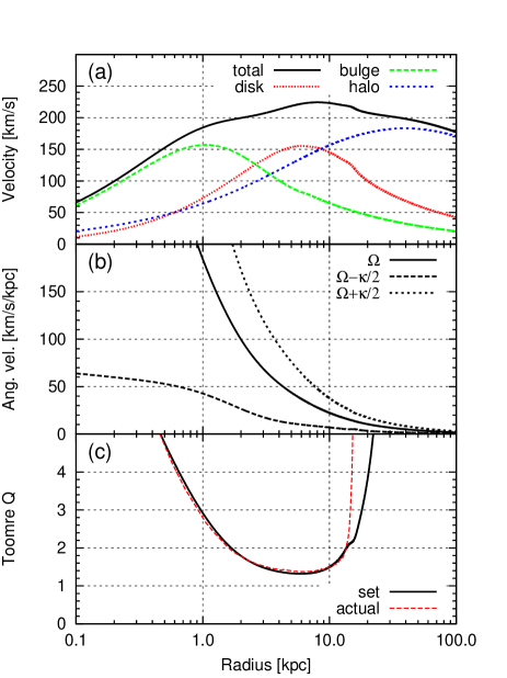
Figure 1: Initial profiles for the basic model: (a) the total circular velocity and its components due to disc, bulge, and halo; (b) angular velocity $\Omega(R)$ and curves $\Omega(R)\pm\kappa(R)/2$; (c) Toomre $Q$ initially set to GalactICS and one actually obtained in the simulations.

The angular velocity profile $\Omega(R)$ is presented in panel (b), along with the curves $\Omega\pm\kappa/2$ which give positions of the inner and outer Lindblad resonances ILR and OLR respectively. The ILR for a pattern speed $\Omega_{\textrm{p}}$ is determined from the relation

$$\Omega_{\textrm{p}}=\Omega_{\textrm{pr}}(R)\equiv\Omega(R)-\frac{1}{2}\kappa(R)\ .$$ (2.3)

Physically, $\Omega_{\textrm{pr}}(R)$ determines a precession rate of nearly circular orbits and plays an important role in the formation of bars in razor thin discs (Polyachenko, 2004); thus one can refer to it as a ‘precession’ curve. For the basic model, the curve diverges weakly at $R\to 0$ as $R^{-\alpha/2}$ with $\alpha\approx 0.5$.

Panel (c) of Fig. 1 shows the Toomre $Q$ profile

$$Q=\frac{\kappa\tilde{\sigma}_{R}}{3.36G\Sigma_{\textrm{d}}}\ ,$$ (2.4)

where $\Sigma_{\textrm{d}}$ is the disc surface density. The profile remains below 3 in the region $1<R<18$ kpc. The minimum $Q_{\textrm{min}}=1.32$ is attained at $R=5.9$ kpc.

3 N-body simulations

Initial conditions of stars in single mass simulations have been generated by the ‘GalactICS’ code provided by Widrow et al. (2008). Numerical calculations have been performed with three different codes.

A particle–mesh code called Superbox-10 (Bien et al. 2013) solves the Poisson equation by fast Fourier transform. The number of grid points $N_{g}$ for each coordinate is the same and is taken so that the number of grid cells is comparable with the number of particles. The code uses grids with three sizes. The largest grid allows one to simulate an extensive halo and interaction between galaxies. Medium-size grids are designed to study separate galaxies and is used for the disc in our case, and the smallest grids are used to resolve fine structures in galactic centres. In all our runs $N_{g}=256$, and the grid radii were 300, 30 and 1 kpc. Effective gravity softening $\epsilon$ in particle–mesh codes is equal to half of the grid cell (Just et al., 2011), so in the centre within 1 kpc $\epsilon\approx 4$ pc, while outside the centre in the disc $\epsilon\approx 117$ pc.

For the largest simulations in our set of runs we use the modification of the recently developed and very popular $N$-body Tree-GPU code implementation bonsai2 (Bédorf et al., 2012a, b), which includes expansion for force computation up to quadrupole order. The code was used with very conservative opening angle ($\theta$ = 0.5) and with the individual gravitational softening option (the softening was set to 10 pc). In our runs we use the simple leap-frog integration scheme with a fixed time-step $\Delta$t = 0.2 Myr to advance the particle positions and velocities during the calculation.

For the simulations of the rigid halo/bulge models and to analyse the snapshot data of all simulations we also use the self coded Tree-GPU based gravity calculation routine ber-gal0 (Zinchenko et al., 2015), which includes expansion for force computation up to monopole order, with the same ($\theta$ = 0.5) opening angle.

In the last years we have already used and extensively tested our hardware accelerator based on the tree gravity calculation routine in a few of our galactic dynamics projects and get quite accurate results with a good performance (Shumakova & Berczik, 2005; Bien et al., 2008; Pasetto et al., 2010, 2011).

The current set of simulations was carried out with the GPU version of the code using local GPU clusters available at the authors’ institutions (ARI: kepler, MAO: golowood, NAOC: laohu) and also the specially dedicated for SFB 881 (“The Milky Way System”) GPU cluster MilkyWay, located in the Jülich Supercomputing Centre in Germany.

3.1 Live disc/bulge/halo runs

Tab. 1 contains parameters of live runs , where all components, disc, bulge and halo, are live, for the basic model. Capital letters denote the numerical code: ‘S’ for Superbox and ‘B’ for bonsai2. Most of the runs have equal mass of the particles within a component, but two runs denoted by ‘m’ have multimass halo particles in order to achieve a better resolution in the bar region. For this, we modified the GalactICS code utilising the same strategy as described in Dubinski et al. (2009). In the region between 0.1 and 1 kpc, the number density ratio of our multimass and single mass runs varies from 10 to 100, thus the effective numerical resolution there is enhanced by this factor.

Run	$N_{\textrm{tot}}$	$N_{\textrm{d}}|N_{\textrm{b}}|N_{\textrm{h}}$	$\epsilon$	e-period	$\Omega_{\textrm{p}}$	$\omega_{\textrm{I}}[B]$	$\omega_{\textrm{I}}$ [E]
S1	5.6	$1.1|0.5|4.0$	4–117	$0.9<t<1.5$	50.6	3.83	$3.66\pm 0.23$
S3m	16.75	$6.0|1.5|9.25$	4–117	$0.9<t<1.5$	52.2	3.59	$3.65\pm 0.25$
B1	5.6	$1.1|0.5|4.0$	10	$0.1<t<1.0$	54.6	4.18	$4.07\pm 0.29$
B2m	16.75	$6.0|1.5|9.25$	10	$0.8<t<1.3$	54.4	4.33	$4.46\pm 0.33$
B3	104.5	$6.0|1.5|97$	10	$0.9<t<1.5$	54.9	4.36	$4.58\pm 0.19$

Table 1: Parameters of live runs of the basic model. Total number of particles $N_{\textrm{tot}}$ and number of particles in components are given in millions (M); gravity softening parameter $\epsilon$ is in pc; e-period – in Gyr; pattern speeds $\Omega_{\textrm{p}}=\omega_{\textrm{R}}/2$ and growth rates $\omega_{\textrm{I}}$ are given in km/s/kpc $\approx$ Gyr^-1. ‘m’ denotes multi mass setup for halo stars.

The total number of particles varies from 5.6M to 104.5M. Our default runs have 16.75M, with 6M particles in the disc, 1.5M in the bulge, and 9.25M in the halo. Runs with smaller and higher number of particles are used to show the effect of an $N$-variation. Mass of halo particles in the B3 run is only twice heavier than the disc and bulge particle mass, so this run is used to show the absence of disc heating from heavier halo particles due to shot noise.

All runs initially show a minor non-equilibrium resulting in a rapid change of the disc thickness and radial redistribution of the central part. So, an average disc height $(\langle z^{2}\rangle)^{1/2}$ within $R_{\textrm{d}}$ is equal to 274 pc at $t=0$, but it is already 290 pc at $t=10$ Myr. Both radial and vertical oscillations disappear during one typical Jeans time $\sim$ 100 Myr. This is a new equilibrium state.

The bar triaxiality parameters of $I_{yy}/I_{xx}$ and $I_{zz}/I_{xx}$, where $I$ are components of the inertia ellipsoid,

$$I_{xx}=\sum\limits_{j}m_{j}x^{2}_{j}\ ,\quad I_{yy}=\sum\limits_{j}m_{j}y^{2}_{j}\ ,\quad I_{zz}=\sum\limits_{j}m_{j}z^{2}_{j}\ ,$$ (3.1)

(with the long axis of the bar oriented along the x-axis) provide the simplest tool to analyse the disc evolution and stability. Here $m_{j}$ denotes the mass of disc particles, and we assume that $j$ spans particles within the characteristic scale length $R_{d}$. In Fig. 2 we show the bar strength defined as

$$B(t)=1-I_{yy}/I_{xx}$$ (3.2)

in linear-log axes for S3m and B2m runs. As a rule, such curves consist of three parts: low amplitude lag, the linear regime growth phases, and plateaus. The latter two are clearly interpreted as exponential growth (its period is indicated as ‘e-period’ in Tab. 1), and saturation of the instability. Note that blue and red curves follow each other even in deep oscillations until $\approx 0.8$ Gyr.

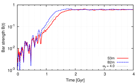
Figure 2: Bar strength in the default live runs S3m and B2m. The dotted line shows growth of the bar strength with rate $4$ Gyr^-1.

The lag part can be short, as in the case of run B1, or last about 1 Gyr (this is the case for the others). During this time, the bar strength increases and decreases, perhaps showing a tendency to increase, but not exponentially. The lag for exponentially fast bar formation can be explained by (i) superposition of modes with different frequencies and azimuthal numbers, or (ii) Poisson noise that operates in stellar systems and affects bar formation. The same lag can be found in Dubinski et al. (2009), Fig. 15, where one can observe a difference between multi-mass 100M run and single mass 100M run (red and black curves respectively). Note that the number of disc particles and initial noise level in these two runs was the same.

After the lag, an instability begins to operate and forms a bar. Fig. 3 shows snapshots at times 1.0, 1.3, 1.6, 2.0, and 4 Gyr of the bar oriented along the $x$-axis.

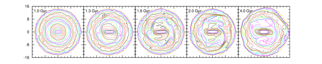
Figure 3: B2m bar patterns oriented along the x-axis at different stages of bar evolution. The curves are isolines of the density evenly spaced in log scale (10 levels for every factor of 10). Each frame size is 32x32 kpc.

Pattern speed $\Omega_{\textrm{p}}$ can be calculated from the change of azimuthal phase of the bar. When the bar amplitude is low, the bar phase is uncertain, so the pattern speed is determined with large errors. During the linear growth, the pattern speed is constant (these values are given in Tab. 1). After the instability saturates, we observe a gradual decrease of $\Omega_{\textrm{p}}$. This effect is known as bar braking.

To quantify the bar shape we fit ellipses to the isophotes and associate a bar radius, $R_{\textrm{b}}$ with the radius at which ellipticity $\varepsilon(r)\equiv 1-b_{e}/a_{e}$ ($a_{e}$ and $b_{e}$ are a major and minor semiaxes of ellipses) declines $\sim$ 15 % from its maximal value (Martinez-Valpuesta et al., 2006). For $t=1$ Gyr, the bar radius is about 1.9 kpc, and $\varepsilon\simeq 0.6$. At the end of the linear growth, $t\approx 1.3$, the bar radius is 4 kpc, with ellipticity 0.72. Some other values are given in Tab. 2.

Time [Gyr]	1.0	1.3	1.6	2.0	2.5	3.0	4.0
$R_{\textrm{b}}$ [kpc]	1.9	4.0	4.9	3.9	2.6	1.8	1.6
$\varepsilon$	0.59	0.72	0.74	0.74	0.76	0.77	0.76

Table 2: Parameters of the bar (radius, ellipticity) in B2m run at different moments in time.

A ratio ${\cal R}$ of the corotation radius $R_{\textrm{c}}$ to the bar radius $R_{\textrm{b}}$ is used to distinguish between fast and slow bars. For usual fast bars, corotation is not far beyond the bar’s end, $1\leq{\cal R}\leq 1.4$ (Debattista & Sellwood, 2000). According to Fig. 4 which shows this ratio as a function of time, ${\cal R}$ reaches one at $t\approx 1.3$ Gyr, and stays there up to $t\approx 1.6$ Gyr. Since the bar slows down after $t\approx 1.3$ Gyr, and thus the corotation radius increases, the bar increases in length during this period and reaches 5 kpc. Afterwards, it begins to shorten.

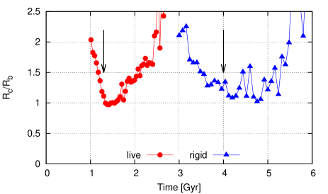
Figure 4: Ratios of the corotation radius $R_{\textrm{c}}$ to the bar radius $R_{\textrm{b}}$ for the default live B2m and default rigid T1r runs. Arrows show the adopted time of saturation of bar instability.

The growth rate can be determined from the slope of the bar strength, $B(t)$, in the linear growth phase. In Tab. 1, this quantity is denoted as $\omega_{\textrm{I}}[B]$. This is close to, but not coincident with the growth rate of the $m=2$ wave amplitudes, which can be measured using a surface density wave amplitude,

$$\tilde{\Sigma}(R)=\frac{1}{\delta M_{\textrm{d}}(R)}\sum_{j}m_{j}\textrm{e}^{-im\theta_{j}}\ ,$$ (3.3)

and radial and azimuthal velocity wave amplitudes:

$$\tilde{V}_{R}(R) =\frac{1}{\delta M_{\textrm{d}}(R)}\sum_{j}m_{j}v_{R,j}\textrm{e}^{-im\theta_{j}}\ ,$$ (3.4)

$$\tilde{V}_{\theta} =V_{\theta}-V_{c}\tilde{\Sigma}(R)\ ,$$ (3.5)

$$V_{\theta}(R) =\frac{1}{\delta M_{\textrm{d}}(R)}\sum_{j}m_{j}v_{\theta,j}\textrm{e}^{-im\theta_{j}}\ ,$$ (3.6)

where $V_{c}=R\Omega(R)$ is the circular velocity, $\delta M_{\textrm{d}}(R)=\sum_{j}m_{j}$ is a mass of particles in a ring of width $\delta R$ near radius $R$. Calculation of growth rates from $N$-body simulations shows $R$-dependence, but it is weak for the particles within the central part of the disc where one global mode dominates. For such cases, we use a mass weighted radial average of these amplitudes in the rings:

$$E(\cdot) =\frac{1}{M_{\textrm{d}}(R_{\textrm{d}})}\sum\delta M_{\textrm{d}}(R)|\cdot|\ ,$$ (3.7)

where $M_{\textrm{d}}(R_{\textrm{d}})=\sum\delta M_{\textrm{d}}(R)$ is a total mass of disc particles within $R_{\textrm{d}}$. The mass weighted radial average for $\tilde{\Sigma}(R)$ gives the usual $A_{2}/A_{0}$ ratio frequently used to characterise the bar mode amplitude (see, e.g., Sellwood, 2016).

Wave amplitudes $E(\tilde{\Sigma}_{\textrm{d}})$, $E(\tilde{V}_{R})$, and $E(\tilde{V}_{\theta})$ are shown in Fig. 5. Comparison with Fig. 2 shows almost the same linear growth from 0.8 to 1.3 Gyr, but smoother behaviour of the wave amplitudes at $t<0.8$ Gyr. The growth rates $\omega_{\textrm{I}}$ inferred from each of the components slightly differ. E.g., for the surface density we obtained 4.33, while for the radial and azimuthal velocity amplitudes they are 4.22 and 4.84 Gyr^-1, respectively. In all runs, $\omega_{\textrm{I}}$ determined from $E(\tilde{\Sigma}_{\textrm{d}})$ and $E(\tilde{V}_{R})$ are close (deviation is 2 per cent), while $\omega_{\textrm{I}}$ inferred from $E(\tilde{V}_{\theta})$ is from 7 to 15 per cent higher. An average value of these three values, along with the corresponding standard deviation, is given as $\omega_{\textrm{I}}[E]$ in Tab. 1.

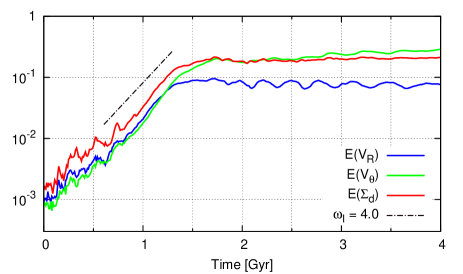
Figure 5: Growth of the wave amplitudes in B2m run. Dash-dotted line shows growth of the bar strength with rate $4$ Gyr^-1. Wave amplitudes are given in N-body units.

The superbox frequencies ($\Omega_{\textrm{p}}$ and $\omega_{\textrm{I}}$) are smaller on average compared to the tree code runs. This can be due to somewhat larger gravity softening of superbox models, since softening makes gravity interaction weaker, and thus one would expect lower frequencies for eigen-oscillations (Polyachenko, 2013). Another explanation can be connected with stochasticity inherent to N-body simulations. Sellwood & Debattista (2009) note that small changes of insignificant parameters can lead to significant changes in galaxy evolution after bar formation. For the S1 run we varied disc inclination relative to the grid, grid flattening, and also made minor changes in distributing particles over the phase space (8 runs including S1 itself). As is seen in Fig. 6, the bar strength curves begin to rise at different times with mean lag $\sim$ 0.6 Gyr.

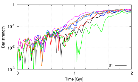
Figure 6: Bar strength curves for S1 model (8 runs which differ insignificantly).

Note that all curves have a low amplitude lag in the beginning, and some even lack the definite linear growth phase. Special methods such as quiet start (Sellwood & Athanassoula, 1986) are used to decrease initial nonaxisymmetric perturbations in order to obtain clear linear growth. We presume that shot noise at some level is an essential ingredient of galaxy dynamics, and thus here we deliberately avoid such procedures as artificial.

The given above analysis and results of others (e.g., Widrow et al., 2008) leave no doubt that bar instability takes place in numerical bars in the presence of ILR (for $\Omega_{\textrm{p}}=55$ km/s/kpc, ILR radius is $\sim 0.4$ kpc), and so discrepancy with the theory needs to be explained.

Axisymmetric properties of the disc do not change until the end of the growth phase, as can be seen in Fig. 7. In the end (1.3 Gyr), the velocity dispersion is affected only within a 2 kpc radius, while the circular velocity is almost preserved, as well as the axisymmetric surface density background. Thus during the growth phase, the stability parameter $Q$ remains unchanged, and one can expect that the main characteristics of the instability (pattern speed, growth rate, shape of the patterns) can be reproduced from linear perturbative analysis. For the moment, however, we are able to calculate linear global modes only for razor-thin discs embedded into a rigid bulge and halo. So, galaxy models with rigid spheroidal components have to be considered.

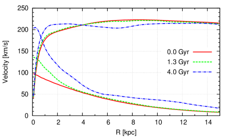
Figure 7: Circular velocity and radial velocity dispersion profiles of the B2m run at 0, 1.3, 4 Gyr.

3.2 Rigid halo/bulge runs

A series of runs with rigid spheroidal components denoted by ‘r’ is presented in Tab. 3. Here ‘S’ again denotes Superbox runs and ‘T’ denotes ber-gal0 Tree code runs. The rigid components were modelled in three ways.

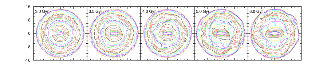
Figure 8: Same as in Fig. 3 for the default rigid run T1r.

Run	$N_{\textrm{tot}}$	$N_{\textrm{d}}|N_{\textrm{b}}|N_{\textrm{h}}$	$\epsilon$	e-period	$\Omega_{\textrm{p}}$	$\omega_{\textrm{I}}[B]$	$\omega_{\textrm{I}}$ [E]
S2r (FP)	5.6	$1.1|0.5|4.0$	4–117	$2.1<t<3.5$	47.8	1.06	$1.09\pm 0.10$
S4r (AX)	1.1	$1.1|-|-$	12	$1.0<t<2.5$	51.1	1.21	$1.12\pm 0.04$
S5r (SP)	1.1	$1.1|-|-$	12	$1.5<t<3.0$	50.2	1.84	$1.51\pm 0.13$
T1r (FP)	16.75	$6.0|1.5|9.25$	10	$2.3<t<3.6$	51.5	1.77	$1.81\pm 0.06$
T2r (SP)	6.0	$6.0|-|-$	10	$2.4<t<3.8$	54.3	1.2	$1.10\pm 0.03$
T3r (AX)	6.0	$6.0|-|-$	10	$2.2<t<3.5$	52.0	1.86	$1.90\pm 0.07$

Table 3: Same as in Tab. 1, for the rigid runs of the basic model.

The simplest but expensive way to simulate galaxies with rigid components is to fix coordinates of bulge and halo particles in space, and use them in calculation of the potential. These runs are S2r and T1r, marked by ‘(FP)’.

In runs marked by ‘(SP)’ (S5r and T2r), halo and bulge potentials are approximated by spherically symmetric functions. The forces from the halo in this case can be calculated analytically, given the NFW potential. The forces from the bulge can be obtained through interpolation from the forces tabulated by integrating density that is given analytically. This is the cheapest but inaccurate way, because in the presence of the disc, distributions of particles in the bulge and halo become axisymmetric rather than spherically symmetric. This manifest itself in larger radial and vertical initial oscillations (e.g., initial disc height jumps from 274 to 305 pc), which are damped after the first $\sim$ 150 Myr.

Finally, in runs marked by ‘(AX)’ (S4r and T3r), halo and bulge potentials are axisymmetric. The potentials and forces from halo and bulge have been tabulated from the actual distribution in the meridian $(R,z)$ plane, and interpolated linearly to positions of disc particles. The initial height jump in this case is the same as in live and (FP) rigid runs, i.e. from 274 to 290 pc.

The superbox runs were made with $N_{\textrm{d}}=1.1\cdot 10^{6}$. The grid sizes for the S2r were 1, 30, 300 kpc, but in S4r and S5r we used another set of grids, 3, 9, 27 kpc, since now there is no need for grids with halo size. Therefore, the effective softening for these runs is only 12 pc. For tree code runs, we used $N_{\textrm{d}}=6\cdot 10^{6}$ particles, with the standard softening $\epsilon=10$ pc.

Fig. 8 shows snapshots of the bar in T1r run (used as a default) oriented along the $x$-axis at times 3, 3.5, 4, 5, and 6 Gyr.

Rigid runs show more extensive lag before the exponential bar growth ($\approx$ 1.9 Gyr on average) than the live runs ($\approx$ 0.6 Gyr). During the lag, the bar strength (Eq. 3.2) and wave amplitudes (Eqs. 3.3–3.6) are not necessarily constant, but rather rise and fall, as shown in Fig. 9. Note also that the end of bar formation is more uncertain in the rigid case. For T1r it can be associated with 3.5 or 4 or even with 5 Gyr, although the linear growth ends at 3.5 Gyr.

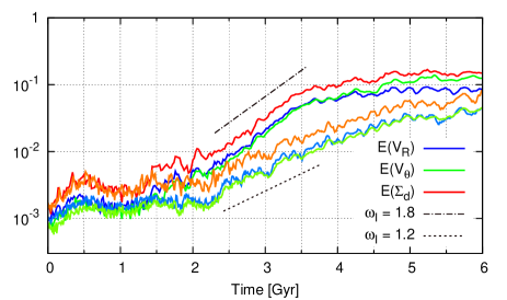
Figure 9: Same as in Fig.5 for the rigid runs T1r (upper group of lines – blue, green, and red) and T2r (lower group of lines – orange, light green, light blue). Dash-dotted and dotted lines show growth with rates 1.8 and 1.2 Gyr^-1.

The pattern speeds $\Omega_{\textrm{p}}$ determined during the e-period (given as ‘e-period’ in the Tab. 3) scatter from 47.8 to 54.3 km/s/kpc. Again, $\Omega_{\textrm{p}}$ is lower for the Superbox code. After the linear growth, the bar slows down in the same manner as in the live runs.

The ratio ${\cal R}=R_{\textrm{c}}/R_{\textrm{b}}$ for the T1r run is shown at Fig. 4 with blue triangles. Compared to the B2m live run, it is more noisy on minimal values, and the minimum is higher, $\sim$ 1.2. The latter is both because the bar is shorter, and the pattern speed is smaller, resulting in larger corotation radius. At the end of bar formation, assumed at $t=4$ Gyr, the bar radius is 3.8 kpc and ellipticity is $\varepsilon=0.65$. The maximum radius of 4.3 kpc is achieved at 4.8 Gyr (ellipticity 0.68). Some other values are given in Tab. 4.

Time [Gyr]	3.0	3.5	4.0	4.5	5.0	5.5	6.0
$R_{\textrm{b}}$ [kpc]	1.8	3.0	3.8	4.1	4.1	2.8	1.7
$\varepsilon$	0.55	0.63	0.65	0.67	0.70	0.72	0.73

Table 4: Parameters of the bar (radius, ellipticity) in T1r run at different moments of time (spline smoothed values).

The growth rates $\omega_{\textrm{I}}$ determined during the e-period spread in the interval from 1.06 to 1.9 Gyr^-1. For each run, the values inferred from the bar strength (Eq. 3.2) and the wave amplitudes (Eqs. 3.3–3.6) are generally in agreement. T1r run, in which rigid components are modelled by fixed particles, gives almost the same frequencies as the T3r run, where halo and bulge are represented by axisymmetric potentials, but different from T2r. Superbox runs are similar: fixed particle (FP) and axisymmetric (AX) runs are close, but the spherically symmetric one is different. One possible reason is that the spherically symmetric runs adjust to a new equilibrium that is different from one in the FP and AX runs. Another, more likely reason is that all runs are subject by stochasticity, which affects not only the lag, but the frequencies as well. Comparison with live runs shows that the stochasticity effect is stronger for less unstable models.

Lower growth rates in the rigid runs are not expected intuitively. One would expect a priori that spherical isotropic (i.e. stable) halos cannot affect disc stability, since the ratio $\rho/\sigma^{2}$ for the disc component is much larger than the same ratio for the halo (Marochnik & Suchkov, 1974). However, the growth rates in runs with live and rigid halos differ by a factor of 2, or even larger. Indeed, while the volume density of halo particles is low in the disc, and their dispersion is high, resonance halo particles are not confined to the disc. Instead, they occupy large resonance regions above and below the disc, and their number and influence turn out to be significant. Considerably weaker bars in the rigid halos were also obtained by Athanassoula (2002), and explained by the additional interaction of the bar with halo particles, mainly on the corotation resonance.

4 Global mode analysis

The confrontation of $N$-body simulations and linear perturbation global mode analysis is a very interesting but challenging problem. As we already mentioned above, direct application of the matrix methods fails in cuspy models because of the presence of an ILR and inability to take into account live halos. Thence, one can try to reproduce modes in $N$-body models with rigid halos, particularly since the pattern speeds are not affected by replacing the live halo with the rigid one.

For bar formation in razor thin discs, it is crucial to have the precession curve $\Omega_{\textrm{pr}}(R)\equiv\Omega(R)-\kappa(R)/2$ with a maximum. If the maximum is not too high, self gravity of the disc is able to support bar-like perturbations with pattern speeds above the maximum (Polyachenko, 2004). This is not the case in cuspy models, where the profile grows infinitely as $r^{-\alpha/2}$ in the centre. One should note however, that $N$-body discs are different from discs considered in linear perturbation analysis, first of all because randomly distributed particles are used to describe the stellar components leading to different stochastic effects. Besides, the potential issues are numerical and depend on equilibrium accuracy, cusp resolution, gravity softening, disc thickness, and the form of the distribution function (DF). All these may distort the precession curve and affect the location of the ILR, important to the appearance of global modes.

4.1 Numerical accuracy

The evaluation of the epicyclic frequency $\kappa$ requires the calculation of a second derivative of the potential:

$$\kappa^{2}=3\Omega^{2}+\Phi^{\prime\prime}\ .$$ (4.1)

If the potential in a particle generator is obtained from some iteration procedure, then $\kappa(R)$ can differ significantly from the cuspy law $\propto r^{-\alpha/2}$. In fact, setting a grid parameter in GalactICS to ordinary $\Delta R=10^{-2}$ one can resolve $\Omega_{\textrm{pr}}(R)$ correctly only until a radius of 0.2 kpc. On smaller radii an artificial maximum of 70 km/s/kpc appears (black solid line in Fig. 10). To get rid of the maximum at least in the range $\Omega_{\textrm{pr}}<100$ km/s/kpc, it is necessary to set this parameter sufficiently small, e.g. $\Delta R=10^{-3}$ (black dashed curve).

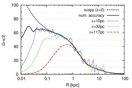
Figure 10: The $\Omega_{\textrm{pr}}$ curves affected by numerical accuracy and softening. The black dashed line shows the true cuspy curve for particles in the equatorial plane, $z=0$; the black solid line shows the curve affected by insufficient numerical accuracy; colour lines show the distortion of the black solid line due to gravity softening.

4.2 Cusp resolution

The number of bulge particles $N_{\textrm{b}}$ can be insufficient to reproduce a cuspy $\Omega_{\textrm{pr}}$ profile. To derive an estimate for a sufficient number of particles, we note that the main uncertainty comes from the calculation of $\kappa$. For spherically symmetric systems, $\kappa^{2}=4\pi G\rho(r)+\Omega^{2}$, thus

$$\frac{\delta\Omega_{\textrm{pr}}}{\Omega_{\textrm{pr}}}\sim\frac{8}{\alpha}\frac{\delta\kappa}{\kappa}\sim\frac{4}{\alpha}\frac{\delta\rho_{\textrm{b}}}{\rho_{\textrm{b}}}\ .$$

The uncertainty of the bulge density $\delta\rho_{\textrm{b}}/{\rho_{\textrm{b}}}$ can be estimated as $(\delta N)^{-1/2}$, where $\delta N$ is the number of particles in a shell of radius $r$ and width $\delta r$, for small radii $\delta N\sim 4\pi N_{\textrm{b}}(r^{2}/R^{3}_{e})\delta r$. If we require the epicyclic frequency to be accurate within a small value $\varepsilon^{\prime}$, the number of particles in the shell should be

$$N_{\textrm{b}}\left(\frac{r}{R_{e}}\right)^{3}\frac{\delta r}{r}\gtrsim(\varepsilon^{\prime}\alpha)^{-2}\ .$$ (4.2)

For example, for $\varepsilon^{\prime}=0.1$ accuracy, to resolve $\Omega_{\textrm{pr}}(R)$ in our model up to $0.1$ kpc, it is sufficient to have 0.2M particles. However, to resolve a radius of 0.05 kpc one needs at least 1.5M particles.

4.3 Gravity softening

A change of the gravity interaction law from the Newton law $r^{-1}$ to a Plummer law $(r^{2}+\epsilon^{2})^{-1/2}$ in Tree codes or the usage of meshes in the particle–mesh code leads to a smearing of the cusp in the density distribution, and consequently to a flattening of the precession profile, i.e. its shape becomes typical for galaxies with cores. These galaxies have finite density and thus obey the solid body rotation law, $\Omega\approx\textrm{const}$, and vanishing $\Omega_{\textrm{pr}}$ in the centre. Fig. 10 shows three examples of $\Omega_{\textrm{pr}}$ calculated for the initial particle distribution in the B2m run, which are affected by 10, 32 and 117 pc softening. For $\epsilon=117$ pc, the obtained profile is 10 per cent lower than the cuspy one already at 1 kpc. For $\epsilon=32$ pc, the $\Omega_{\textrm{pr}}$ falls off the correct profile at $R\approx 0.5$ kpc, and peaks at 0.2 … 0.3 kpc. The value of $\epsilon=10$ pc adopted in our Tree code simulations alters the profile given by the black solid curve only within $R<0.03$ kpc.

In our calculations we use $N_{\textrm{d}}=1.1$M and 6M particles to represent the disc component, and $N_{\textrm{b}}=0.5$M and 1.5M particles to represent the bulge component. A natural condition for the softening is that softening volume should contain several particles to properly suppress both potential fluctuations and 2-body scattering at short range. For disc particles $a^{3}N_{\textrm{d}}\sim(z_{\textrm{d}}R^{2}_{\textrm{d}})$, which gives for a mean distance between particles $a\sim(z_{\textrm{d}}R^{2}_{\textrm{d}}/N_{\textrm{d}})^{1/3}=8...14$ pc. An estimate for the bulge gives $a\sim(R^{3}_{e}/N_{\textrm{b}})^{1/3}=6...11$ pc. Thus, our choice of $\epsilon=10$ pc is sufficiently large for the default runs, but may be a source of some relaxation in models with a smaller number of particles.

Large values of the gravity softening parameter $\epsilon$ should also affect the equilibrium, since GalactICS lacks this parameter. We expect, however, that it happens when $\epsilon$ becomes a noticeable fraction of the characteristic scales, which are of the order of 1 kpc.

4.4 Thickness

In contrast to razor thin discs used in linear perturbation analysis, real discs and their $N$-body counterparts are three-dimensional. While motion in the plane is always integrable, in the sense that the Hamilton–Jacobi equation separates leading to periodic radial and azimuthal motion, this is not generally the case in 3D motion. It is likely that the orbits of many disc particles remain regular, i.e. they respect three integrals of motion and have three fundamental frequencies. However, direct integration of orbits shows that for particles with $R\lesssim z\sim z_{d}$, the radial frequency is no longer fundamental, but rather a combination of frequencies. So, the radial frequency $\Omega_{R}$, as well as the usual ILR, is not defined at $R\lesssim z_{d}$. Certainly, for larger radii, $R\gg z_{d}$, the motion is nearly flat, and usual frequencies can be introduced. For example, for nearly circular orbits in the $z=0$ plane the vertical motion can be separated so that particles oscillate in a ‘vertical’ potential $\Phi(R,z)-\Phi(R,0)$. However, in the case $R\lesssim z_{d}$ the ILR should be substituted by a resonance with a different combination of frequencies, and interaction with waves on this resonance should be reconsidered.

To proceed further, we consider a simple model that allows replacing the complex 3D orbital motion with planar motion. Only a small fraction of particles that travel close to the galactic symmetry plane $z=0$ feels the cuspy form of the $\Omega_{\textrm{pr}}$ profile. Angular velocity $\Omega$ and epicyclic frequency $\kappa$ out of that plane do not have a cuspy singularity $r^{-\alpha/2}$, since

$$\Omega^{2}(R,z)=\frac{1}{R}\frac{\partial\Phi(R,z)}{\partial R}\ ,$$ (4.3)

and $\Phi(R,z)$ is smooth at $R=0$ if $z\neq 0$. Thus nearly all particles move as if there is a cored rather than cuspy $\Omega_{\textrm{pr}}$ profile. Fig. 11 shows precession curves calculated for different height $z$ of the initial distribution of the B2m run (each thin line represents $\Omega_{\textrm{pr}}(R)$ calculated for particles in a flat layer with a thickness of 50 pc), and the averaged profile

$$\overline{\Omega}_{\textrm{pr}}=\overline{\Omega}-\overline{\kappa}/2\ ,$$ (4.4)

where overlines denote square averages, i.e. $(\overline{\Omega})^{2}=\langle\Omega^{2}\rangle_{z}$ and $(\overline{\kappa})^{2}=\langle\kappa^{2}\rangle_{z}\equiv 4\langle\Omega^{2}\rangle_{z}+d\langle\Omega^{2}\rangle_{z}/dr$. The maximum of the averaged curve turns out to be 43.7 km/s/kpc at 0.52 kpc, which is well below the pattern speed obtained in our simulations with rigid halos. The effective precession curve roughly coincides with the curve calculated for particles that are $z\sim 150...200$ pc out of the plane.

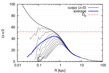
Figure 11: The precession profiles of the B2m initial distribution calculated for different elevations of particles above the plane (each thin solid curve is calculated for particles in the layer $\Delta z=50$ pc width, starting from $z=0$), and average $\overline{\Omega}_{\textrm{pr}}$ (thick solid curve). The dashed line shows the cuspy profile for particles in the the equatorial plane. The dash-dotted line shows the bar pattern speed obtained in rigid halo models.

4.5 The Distribution function

The disc phase space distributions used in GalactICS with the form $f_{0}(R,z,v_{R},v_{\theta},v_{z})$ cannot be reproduced by DFs with the form $F_{0}(E,L_{z})$ or $F_{0}(J_{r},L_{z})$ used in matrix methods, since they do not account for the vertical motion. Even if one neglects the vertical motion and considers the Schwarzschild DF

$$f_{0}(R,v_{R},v_{\theta})=\left.\frac{\Omega}{\pi\kappa}\frac{\Sigma_{\textrm{d}}}{\tilde{\sigma}^{2}_{R}}\right|_{R}\exp\left(-\frac{v^{2}_{R}+\gamma^{2}\tilde{v}^{2}_{\theta}}{2\tilde{\sigma}_{R}^{2}(R_{c})}\right)\ ,$$ (4.5)

(here $\tilde{v}_{\theta}\equiv v_{\theta}-R\Omega(R)$, $\gamma\equiv 2\Omega/\kappa$) for particles confined to the $z=0$ plane, there are many ways to approximate this function by a DF with two integrals of motion. A frequently used form is

$$F_{0}(E,L_{z})=\left.\frac{\Omega}{\pi\kappa}\frac{\Sigma_{\textrm{d}}}{{\tilde{\sigma}}^{2}_{R}}\right|_{R_{c}}\exp\left(-\frac{E-E_{c}(L_{z})}{\tilde{\sigma}_{R}^{2}(R_{c})}\right)\ ,$$ (4.6)

where $R_{c}(L_{z})$ and $E_{c}(L_{z})$ are the radius and energy of a particle on a circular orbit with angular momentum $L_{z}$. $\Omega(R_{c}(L_{z}))$ and $\kappa(R_{c}(L_{z}))$ are determined by the total gravitational potential, which is a free input function. The function (Eq. 4.6) is close to (Eq. 4.5) when the radial velocity dispersion $\tilde{\sigma}_{R}$ is small, but for real dispersions the difference in the inner disc can be significant. Besides, function (Eq. 4.6) is an even function of $L_{z}$, thus, for example, its values on lines of prograde and retrograde circular orbits coincide. This calls for using various taper functions curving out a fraction of retrograde and nearly radial orbits, which add an uncertainty to the study. Another way to account for the retrograde orbits and to approximate DF (Eq. 4.5) without using taper functions is to consider $R_{c}$ as a function of $E$. Using a relation $E-E_{c}\approx(L_{c}-L)\Omega(R_{c})$ valid for small $\tilde{\sigma}$, we replace (Eq. 4.6) with a DF with the form:

$$F_{0}(E,L_{z})=\left.\frac{\Omega}{\pi\kappa}\frac{\Sigma_{\textrm{d}}}{\tilde{\sigma}^{2}_{R}}\right|_{R_{c}}\exp\left([L-L_{c}(E)]\frac{\Omega(R_{c})}{\tilde{\sigma}_{R}^{2}(R_{c})}\right)\ ,$$ (4.7)

where now $\Omega=\Omega(R_{c}(E))$, $\kappa=\kappa(R_{c}(E))$.

4.6 Bar mode of the basic model

For the global mode calculation we adopt a DF in the form (Eq. 4.7) that includes both prograde and retrograde orbits; an effective potential corresponding to the averaged radial force, and averaged profile (Eq. 4.4); the surface density and radial velocity dispersion profiles inferred from the initial distribution averaged over the vertical axis.

Here we use a matrix method by Polyachenko (2005) that has a form of the linear matrix equation,

$${\mathbf{A}}{\mathbf{x}}=\omega{\mathbf{x}}\ ,$$ (4.8)

which allows us to find unstable modes effectively without a priory information on the localisation of modes.

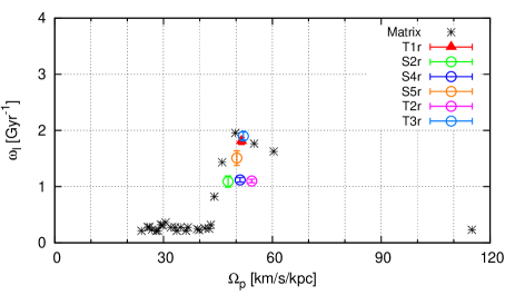
Figure 12: Disc eigenmodes of the basic model obtained with the matrix method.

$\Omega_{\textrm{p}}$	60.4	55.0	49.8	46.2	44.0
$\omega_{\textrm{I}}$	1.63	1.77	1.95	1.43	0.82
CR	3.48	3.86	4.32	4.70	4.96
OLR	6.37	7.00	7.71	8.28	8.67

Table 5: Unstable global modes (pattern speed $\Omega_{\textrm{p}}$, and growth rate $\omega_{\textrm{I}}$ in km/s/kpc $\approx$ Gyr^-1; resonance radii – in kpc) for the basic model ($z_{\textrm{d}}=300$ pc, maximum of the averaged $\Omega_{\textrm{pr}}$ profile is 43.7 km/s/kpc) obtained with the matrix method.

The obtained spectrum consists of two groups of modes (Fig. 12). The faster rotating modes with $\Omega_{\textrm{p}}>80$ km/s/kpc are localised between corotation resonance CR and OLR, and they are out of the scope of what we study here. In the slower rotating group we see several dominating modes. All unstable matrix modes (Table 5) lack the ILR, which is consistent with the standard point of view on the ILR as a damping agent. Their growth rates are 0.8 … 2 Gyr^-1, i.e. they coincide with the values obtained in rigid halo/bulge $N$-body simulations. The $N$-body pattern speed of 52 km/s/kpc is a mean value of the matrix pattern speeds, so the bar mode can be a superposition of matrix modes.

Patterns of the matrix modes are presented in Fig. 13. They look like lumpy structures with different numbers of maxima spaced by approximately 90 degrees. Modes with larger growth rates are more likely to be dominant, thus it is natural to expect the observed pattern speed to be between 49.8 and 55 km/s/kpc. Each of the frames shown in Fig. 8 is a superposition or nonlinear evolution of these modes.

The bar diagrams below the patterns indicate angular momentum exchange in the modes above. Each bar is proportional to Fourier components of angular momentum $L_{m}(l)$, normalised so that the sum of the positive components equals one. The Fourier components,

$$L_{m}(l)=-\int{\rm d}{\mathbf{J}}F^{\prime}_{0,l}(J)\frac{|\Psi_{l}({\mathbf{J}})|^{2}}{|\omega-l\Omega_{1}({\mathbf{J}})-m\Omega_{2}({\mathbf{J}})|^{2}}\$$ (4.9)

obey the angular momentum conservation law, $L_{m}=\sum_{l}L_{m}(l)=0$. In the expression, $\Omega_{1}$ and $\Omega_{2}$ are radial and angular frequencies of a particle in the orbit ${\mathbf{J}}=(J_{R},L_{z})$, $J_{R}$ is the radial action, and $L_{z}$ is the $z$ component of the angular momentum. Other entities are explained in Polyachenko & Just (2015, Sect. 2.2). Contribution to each bar comes mainly from the region where the corresponding denominator peaks. For $l=-1$ substitution $\omega=m\Omega_{\textrm{p}}+\textrm{i}\omega_{\textrm{i}}$, and $m=2$ gives the peak where $|\Omega_{\textrm{p}}-(\Omega_{2}-\Omega_{1}/2)|$ is the smallest, i.e. in the vicinity of the precession curve maximum. Similarly, $l=0$ and $l=1$ bars contribute mainly corotation and OLR regions. Thus, we conclude from the bar charts that the angular momentum exchange occurs mainly between stars in the vicinity of the precession curve maximum and stars on corotation and OLR resulting in a net outward flow of angular momentum.

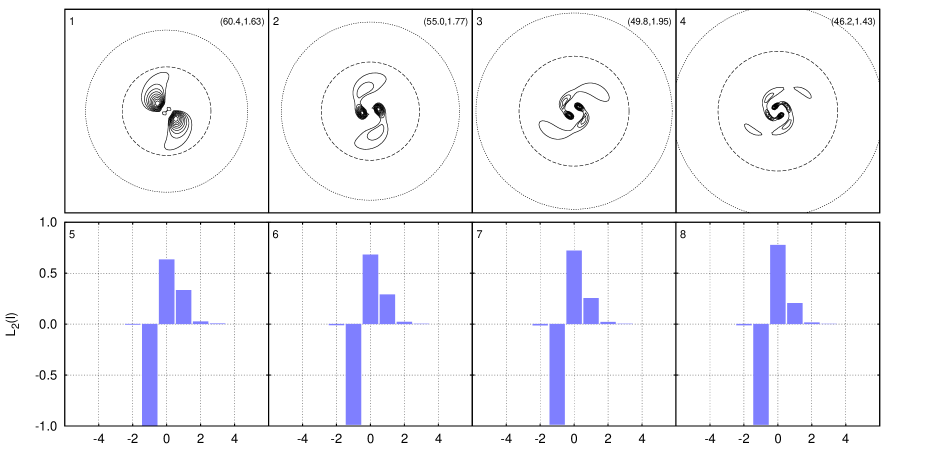
Figure 13: The matrix modes. Frames (1–4): patterns of the most unstable modes. Isolines show the excess surface density over the axially symmetric distribution by 10, 20, … 90 per cent. The pattern speeds and the growth rates are given in parentheses, $(\Omega_{\textrm{p}},\omega_{\textrm{I}})$. Dashed lines show CR, while dotted lines show the Lindblad resonances. Each frame size is 16x16 kpc. Bars (5–8) indicate the dependence of $L_{2}(l)$ vs. $l$ reflecting angular momentum exchange between different parts of the disc.

4.7 Different vertical scales

In this section we compare N-body and matrix modes for the discs with different thickness controlled by the vertical scale parameter $z_{d}$. An initial range of $z_{d}$ was narrowed to $100...400$ pc. The disc with $z_{d}=100$ pc is an outlier in our N-body analysis, and it suffers from buckling instability. Discs with $z_{d}>400$ pc turned out to be stable.

We performed two series of N-body simulations with axisymmetric halo and bulge potentials using ber-gal0 Tree code, with $N_{\textrm{d}}=6$M and 3M particles. The obtained N-body modes, along with the matrix modes, are presented in Tab. 6 and shown in Figs. 14, 15.

Modes	$z_{d}$ [pc]	100	150	200	250	300	350	400
6M	$\Omega_{\textrm{p}}$	–	56.9	56.7	55.0	52.0	50.3	47.0
	$\omega_{\textrm{I}}$ (B)	–	2.58	2.69	2.50	1.86	1.23	1.05
	$\omega_{\textrm{I}}$ (E)	$2.56\pm 0.20$	$1.81\pm 0.12$	$2.15\pm 0.17$	$2.20\pm 0.09$	$1.74\pm 0.07$	$1.22\pm 0.01$	$1.13\pm 0.03$
3M	$\Omega_{\textrm{p}}$	59.7	56.2	56.0	54.2	52.1	50.2	48.3
	$\omega_{\textrm{I}}$ (B)	2.91	1.72	2.61	2.27	2.20	1.36	1.13
	$\omega_{\textrm{I}}$ (E)	$2.29\pm 0.20$	$1.45\pm 0.16$	$2.08\pm 0.08$	$2.15\pm 0.09$	$2.09\pm 0.02$	$1.26\pm 0.04$	$1.15\pm 0.03$
Matrix	$\Omega_{\textrm{p}}+\textrm{i}\omega_{\textrm{I}}$	64.8 + 1.25i	63.2 + 1.43i	62.3 + 1.54i	61.2 + 1.55i	60.4 + 1.63i	59.5 + 1.56i	58.9 + 1.65i
	$\Omega_{\textrm{p}}+\textrm{i}\omega_{\textrm{I}}$	59.9 + 1.61i	58.3 + 1.48i	57.1 + 1.77i	56.0 + 1.72i	55.0 + 1.77i	54.1 + 1.96i	53.3 + 1.97i
	$\Omega_{\textrm{p}}+\textrm{i}\omega_{\textrm{I}}$	55.0 + 1.51i	53.4 + 1.51i	52.0 + 1.87i	50.8 + 2.05i	49.8 + 1.95i	48.9 + 2.07i	48.1 + 2.16i
	$\Omega_{\textrm{p}}+\textrm{i}\omega_{\textrm{I}}$	51.4 + 1.08i	50.0 + 1.30i	48.4 + 1.44i	47.2 + 1.32i	46.2 + 1.43i	45.3 + 1.30i	44.5 + 1.45i

Table 6: N-body (6M and 3M) and matrix modes. For N-body modes, growth rates are calculated using both the bar strength (Eq. 3.2) (denoted by [B]) and wave amplitudes (Eqs. 3.3–3.6), denoted by [E].

Fig. 14 shows pattern speeds of the modes. For each $z_{d}$ we have four modes with the highest growth rates which were used to calculate a pattern speed as an average weighted by the growth rates. These pattern speeds are then used to calculate a smooth fit (black solid curve). Upper and lower limits of the red error bars show pattern speeds of modes with the largest growth rates. As expected, matrix modes appear above the maxima of the precession curves. N-body modes agree well with the matrix calculations.

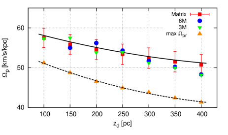
Figure 14: The pattern speeds of matrix and N-body modes calculated in $N_{\textrm{d}}=6$M and 3M runs. Upper and lower limits of the red error bars show pattern speeds of modes with the largest growth rates. Orange upward triangles show maxima of the precession curves for each $z_{d}$. Black dashed line shows a smooth fit to the triangles. Black solid curve shows a smooth fit to the average pattern speeds of matrix modes.

Fig. 15 shows growth rates of the modes. For each $z_{d}$ we have shown two maximum growth rates (upper and lower limits of the error bars). The growth rates were calculated using bar strength (Eq. 3.2) and wave amplitudes (Eqs. 3.3–3.6), in both series of N-body runs. The growth rates obtained with the two methods are quite close. Comparison with matrix equations shows good agreement for 150, 250, 300 pc runs. The model with 100 pc is an outlier, for a reason which is not well understood. In particular, for 6M run we were unable to determine the pattern speed and growth rate $\omega_{\textrm{I}}[E]$. For the thicker discs, $z_{d}\geq 350$ pc, N-body shows a decrease of the instability, while the matrix method shows a weak trend of instability increase. A possible reason for the different trends is an effect of increasing vertical velocity dispersion that act similar to the radial velocity dispersion and stabilise the disc, which is not included in the martix method.

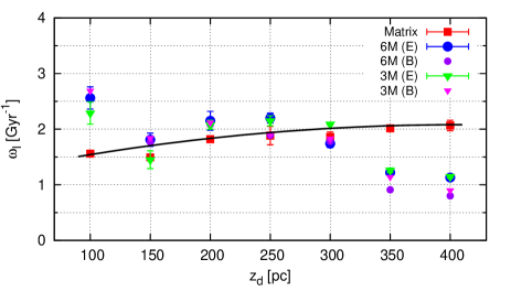
Figure 15: The growth rates of matrix and N-body modes calculated in $N_{\textrm{d}}=6$M and 3M runs. Upper and lower limits of the red error bars show two maximum growth rates. 6M(E) and 3M(E) show the rates obtained with wave amplitudes (Eqs. 3.3–3.6), while 6M(B) and 3M(B) show the rates obtained with bar strength (Eq. 3.2) using 6M and 3M N-body runs.

5 Discussion and Conclusions

In this paper we study bar formation in a galactic model with a cusp and other parameters which our Galaxy possibly possesses. The model consists of three stellar components: exponential disc, cuspy bulge, and NFW halo. Our study includes $N$-body simulations with particle–mesh (PM) and Tree codes, and the calculation of global modes.

First of all, using one ‘basic’ model and more than 100M particles, we definitely show that a bar really forms despite the presence of the ILR. This is the case in live and rigid halo and bulge runs. Maximum bar radius is achieved soon after saturation of the instability. In the live runs it is around 5 kpc, with ellipticity of about 0.75 (Tab. 2). In the rigid runs, the obtained bars are somewhat shorter and rounder: maximum radius is 4.3 kpc, with ellipticity 0.68 (Tab. 4).

Substitution of halo and bulge particles with the rigid external potential revealed that rigid cuspy models are less unstable than live ones, i.e. typical growth rates are twice as small. This is in agreement with results by Athanassoula (2002) obtained for the bulgeless models. At the same time, pattern speeds in live and rigid runs are close (relative difference is 5 per cent or less).

Stochastic behaviour of N-body models, mentioned e.g. by Sellwood & Debattista (2009) for disc evolution after bar formation, is also seen in our runs, especially in the case of the rigid halo and bulge, when growth rates are small. This manifests itself in appearance of the random lag before the exponential growth of the amplitude, and sometimes in the non-exponential character of the growth. Special techniques are used to obtain models that demonstrate more evident exponential growth Sellwood & Athanassoula (e.g. 1986), but here we avoid using it emphasising that stochasticity and shot noise are inherent properties of the stellar systems.

The models demonstrating the exponential growth preserve initial axisymmetric parameters quite well so that the Toomre $Q$ parameter remains unchanged almost until saturation. This fact allows one to calculate unstable global modes using matrix methods of linear perturbative analysis, and compare them with rigid N-body runs. While using the cuspy potential in the equatorial plane, no unstable modes are found by the matrix method (Polyachenko, 2005).

For usual bar mode instability in thin discs, the behaviour of the $\Omega_{\textrm{pr}}$ profile determining the position of the ILR is important. We emphasise that the resonance radius for the ILR is well defined only for nearly circular motion in razor thin discs. For eccentric orbits in the plane, the ILR is a curve in action space. If the orbit is not planar, frequencies determining the ILR can be approximated if radius $R$ is much larger than the maximum elevation $z$ above the plane. However, if $R\lesssim z_{\textrm{d}}$, the orbit is essentially 3-dimensional and generally not quasiperiodic. Thus, at radii $R\lesssim z_{\textrm{d}}$, the resonances are smeared out and the appeal of an ILR is meaningless.

Using a toy model that averages radial forces along the axis perpendicular to the disc plane, we obtain an effective potential and $\Omega_{\textrm{pr}}(R)$ that possesses a maximum. In other words, the obtained precession curve is typical for cored models, which allows for the unstable modes. The obtained global modes in models with various vertical scales in the range $100\leq z_{d}\leq 400$ pc agree well with the $N$-body calculations.

Matrix calculations show strong dependence of the growth rates from the disc mass. For example, for $M_{\textrm{d}}$ only 11 per cent lower than adopted in our models, the obtained growth rates are 2.5 times smaller. If one can extrapolate these results to live discs preserving the ratio of the growth rates of the live and rigid models at factor of 2, it means that the galactic disc remains nearly stable (instability time is larger than age of the Universe) for a long time, and the bar started to form only recently. Our crude estimates using reasonable star formation rates show that during 10 Gyr small disc perturbations grow by a factor $\exp(5...6)$ which is needed for the Poisson noise of the disc consisting of $N_{\textrm{d}}\sim 10^{6}$ particles to grow into a bar. This fact can explain the observed lack of barred galaxies at redshifts $z\gtrsim 0.5$ (Abraham et al., 1999; Merrifield et al., 2000), and typical ratios of corotation to bar radii, $0.9<{\cal R}<1.3$ (Binney & Tremaine, 2008), as a sign of relatively young bars close to their maximum size.

In this paper we have revealed an ILR is practically non-existent, taking into consideration the thickness of the disc. On the other hand, according to the WASER theory (e.g., Bertin, 2014), unstable modes could be excited if there is an inner Q-barrier and such a barrier shields the existing ILR. In fact, a cubic dispersion relation by Bertin et al. (1989) gives one ‘shielded’ mode with the pattern speed $\Omega_{\textrm{p}}=55$ km/s/kpc, i.e. very close to predictions of N-body simulations and matrix equations (shielding starts from 44 km/s/kpc). In a separate paper we plan to explore WASER mechanism in more detail using models with different radial velocity dispersions.

References

- Abraham et al. (1999) Abraham R.G. et al., 1999, MNRAS, 308, 569
- Antoja et al. (2014) Antoja, T. et al., 2014, A&A, 563, 60
- Athanassoula (2002) Athanassoula E., 2002, ApJ, 569, 83
- Bédorf et al. (2012a) Bédorf J., Gaburov E., Portegies Zwart S., 2012a, in Astronomical Society of the Pacific Conference Series, Vol. 453, Advances in Computational Astrophysics: Methods, Tools, and Outcome, Capuzzo-Dolcetta R., Limongi M., Tornambè A., eds., p. 325
- Bédorf et al. (2012b) Bédorf J., Gaburov E., Portegies Zwart S., 2012b, Bonsai: N-body GPU tree-code. Astrophysics Source Code Library
- Bertin et al. (1989) Bertin G., Lin C.C., Lowe S.A., Thurstans R.P., 1989, ApJ 338, 104
- Bertin (2014) G. Bertin, Dynamics of Galaxies (Cambridge : Cambridge University Press, 2014).
- Bien et al. (2008) Bien R., Just A., Berczik P., Berentzen I., 2008, Astronomische Nachrichten, 329, 1029
- Bien (2013) Bien R., Brandt T., Just A., 2013, MNRAS, 428, 1631
- Binney & Tremaine (2008) J. Binney, S. Tremaine,Galactic Dynamics (Princeton : Princeton University Press, 2008).
- Chemin et al. (2015) Chemin, L. et al., 2015, A&A, 578, id.A14, 8
- Debattista & Sellwood (2000) Debattista V.P., Sellwood J.A., 2000, ApJ, 543, 704
- Diemand et al. (2008) Diemand J. et al., 2008, Nature, 454, 735
- Dubinski et al. (2009) Dubinski J., Berentzen I., Shlosman I., 2009, ApJ, 697, 293
- Evans & Read (1998) Evans N.W., Read J.C.A., 1998, MNRAS 300, 106
- Fridman & Polyachenko (1984) Fridman A.M., Polyachenko V.L., 1984, Physics of Gravitating Systems, Springer, New York
- Golubov& Just (2013) Golubov O., Just A., 2013, IAUS, 295, 231
- Hohl (1971) Hohl F., 1971, ApJ 167, 343
- Jalali (2010) Jalali M.A., 2010, MNRAS 404, 1519
- Just et al. (2011) Just A., Khan F. M., Berczik P., Ernst A., Spurzem R., 2011, MNRAS 411, 653
- Kormendy (2013) Kormendy J. Secular Evolution of Galaxies (Cambridge : Cambridge University Press, 2013)
- Mark (1971) Mark J. W.-K., 1971, Proc. Natl. Acad. Sci. USA, 68, 2095
- Mark (1974) Mark J. W.-K., 1974, ApJ, 193, 539
- Marochnik & Suchkov (1974) Marochnik L.S., Suchkov A.A., 1974, Sov. Phys. Usp. 17, 85
- Martinez-Valpuesta et al. (2006) Martinez-Valpuesta I., Shlosman I., Heller C., 2006, ApJ, 637, 214
- Merrifield et al. (2000) Merrifield, M. R., 2000, ASP Conf. Ser., 197, 39
- Miller et al. (1970) Miller R.H., Prendergast K.H., Quirk W.I., 1970, ApJ, 161, 903
- Moetazedian & Just (2016) Moetazedian R., Just A., 2016, MNRAS, 459, 2905
- Pasetto et al. (2011) Pasetto S., Grebel E. K., Berczik P., Chiosi C., Spurzem R., 2011, A&A, 525, A99
- Pasetto et al. (2010) Pasetto S., Grebel E. K., Berczik P., Spurzem R., Dehnen W., 2010, A&A, 514, A47
- Polyachenko (2004) Polyachenko E. V., 2004, MNRAS, 348, 345
- Polyachenko (2005) Polyachenko E. V., 2005, MNRAS, 357, 559
- Polyachenko (2013) Polyachenko E. V., 2013, Astron. Lett., 39, 72
- Polyachenko & Just (2015) Polyachenko E. V., Just A. 2015, MNRAS, 446, 1203
- Sellwood (2000) Sellwood J., 2000, ASP Conf. Ser., 197, 2
- Sellwood & Athanassoula (1986) Sellwood J.A., Athanassoula E., 1986, MNRAS, 221, 195
- Sellwood & Debattista (2009) Sellwood J.A., Debattista V.P., 2009, MNRAS, 398, 1279
- Sellwood (2016) Sellwood J., 2016 ApJ, 819, 92
- Shumakova & Berczik (2005) Shumakova T. A., Berczik P. P., 2005, Kinematika i Fizika Nebesnykh Tel, 21, 288
- Sofue et al. (2009) Sofue, Y., Honma, M., Omodaka, T. 2009, PASJ 61, 283
- Toomre (1977) Toomre A., 1977, ARA&A 15, 437
- Toomre (1981) Toomre A., Structure and evolution of normal galaxies (Ed. S.M. Fall and D. Lynden-Bell, Cambridge Univ. Press., 1981), p.111.
- Widrow et al. (2008) Widrow L. M., Pym B., Dubinski J., 2008, ApJ, 679, 1239
- Zinchenko et al. (2015) Zinchenko, I. A., Berczik, P., Grebel, E. K., Pilyugin, L. S., Just, A., 2015, ApJ 806, 267