Efficient 2D-to-3D Deformable Shape Matching for 3D Shape Retrieval Applications

Abstract

We discuss an algorithm for non-rigid 2D-to-3D shape matching, where the input is a 2D query shape as well as a 3D target shape and the output is a continuous matching curve represented as a closed contour on the 3D shape. We cast the problem as finding the shortest circular path on the product 3-manifold of the two shapes. We prove that the optimal matching can be computed in polynomial time with a (worst-case) complexity of $\mathcal{O}(mn^{2}\log(n))$ where $m$ and $n$ denote the number of vertices on the 2D and the 3D shape respectively. Computing a solution with a relative error of $\epsilon$ has the same complexity but ensures faster convergence in some cases. Quantitative evaluation confirms that the method provides excellent results for sketch-based deformable 3D shape retrieval.

1 Introduction

The last decade has witnessed a tremendous growth in the quantity and quality of geometric data available in the public domain. One of the driving forces of this growth has been the development in 3D sensing and printing technology, bringing affordable sensors such as Microsoft Kinect or Intel RealSense and 3D printers such as MakerBot to the mass market. The availability of large geometric datasets brings forth the need to explore, organize, and search in 3D shape collections, ideally in the same easy and efficient way as modern search engines allow to process text documents.

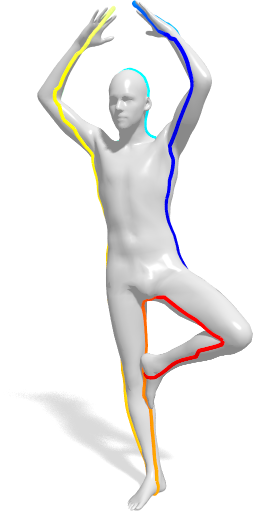
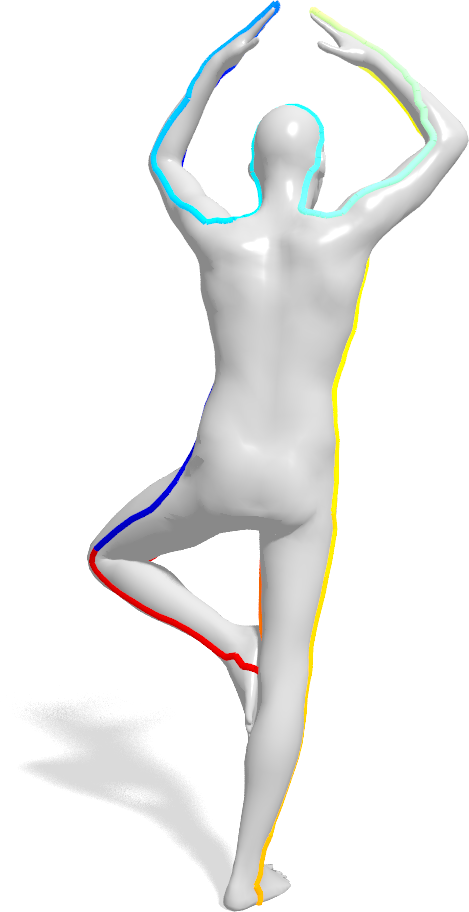
Figure 1: We propose a shape matching method between a 2D query shape (left) and a 3D target shape (right), both of which are allowed to deform non-rigidly. The globally optimal matching (shown on top of the 3D target) is guaranteed to be continuous.

Numerous works on content-based shape retrieval funkhouser2003search ; tangelder2008survey ; bronstein2011shape try to extend popular search paradigms to a setting where the 3D query shape is matched to shapes in the database using some criterion of geometric similarities. Typically, a 3D shape is represented as a descriptor vector aggregating some local geometric features, and retrieval is done efficiently by comparing such vectors bronstein2011shape . However, the need for the query to be a 3D shape significantly limits the practical usefulness of such search engines: non-expert human users are typically not very skilled with 3D modeling, and thus providing a good query example can be challenging. As an alternative to 3D-to-3D shape retrieval, several recent works proposed 2D-to-3D or sketch-based shape retrieval, where the query is a 2D image representing the projection or the silhouette of a 3D shape as seen from some viewpoint eitz2012sbsr ; furuya14 ; Li20151 ; su15mvcnn ; hueting2015crosslink . This setting is much more natural to human users who in most cases are capable of sketching a 2D drawing of the query shape; however, the underlying problem of ‘multi-modal’ similarity between a 3D object and its 2D representation is a very challenging one, especially if one desires to deal with non-rigid shapes such as human body poses. In fact, so far all methods for 2D-to-3D matching have limited the attention to rigid shapes such as chairs, cars, etc.

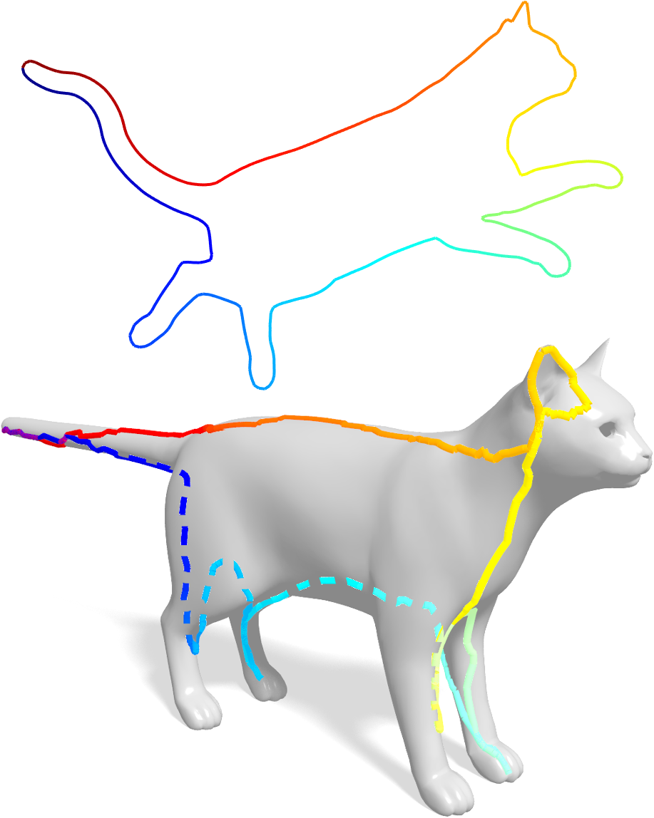
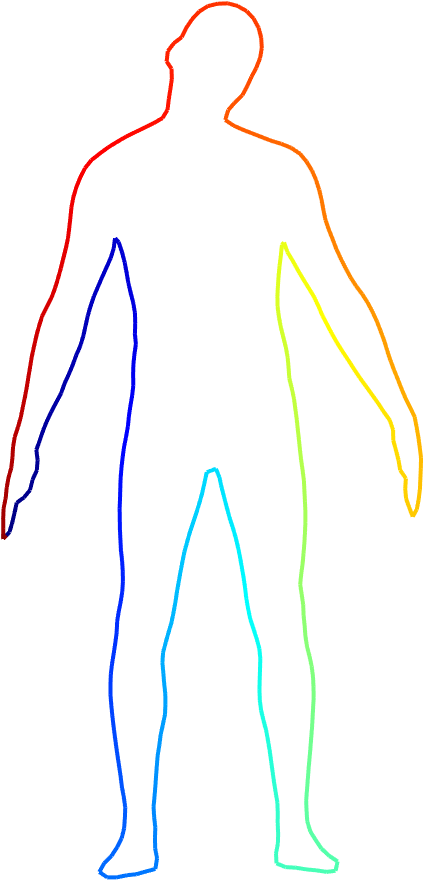
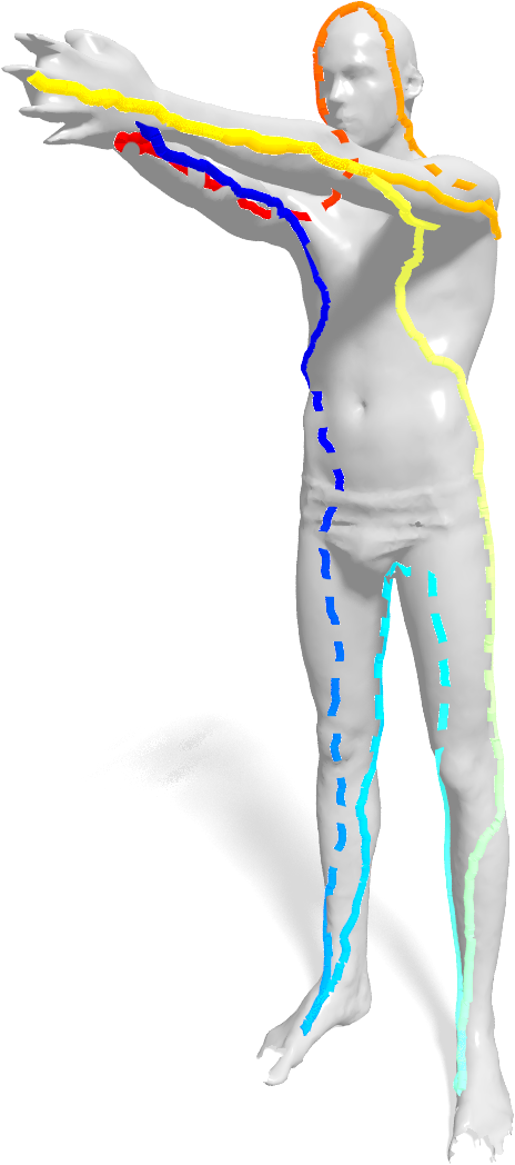
Figure 2: Examples of correspondences between a cat contour and a 3D cat (left) and human contours and 3D humans (middle and right). The human shape (middle) exhibit a topological change along the hands which is handled well by our method. The contour on the right is handdrawn. The dashed lines denotes correspondences that are normally not visible from this point of view.

Here, we propose a method for automatically finding correspondence between 2D and 3D deformable objects. To the best of our knowledge, this is the first method to address the problem in the deformable setting. Prior approaches to the 2D-to-3D matching problem were limited to the less challenging rigid setting. The input to our algorithm is a 2D query curve and a 3D target surface, and the output is the corresponding continuous curve on the surface (see Fig. 1). Our method can either guarantee a globally optimal solution or an $\epsilon$-approximation of it, and has polynomial time complexity. The $\epsilon$-tight solution comes with decreased runtime and slightly less precision but this does not actually corrupt the retrieval results too much. In practice, we observe computationally efficiency with 1-20 seconds for running the complete pipeline to got a matching of shapes up to $40,000$ vertices. Additionally, our approach allows using different local feature descriptors for 2D and 3D data. In particular, we show how spectral 2D and 3D features can be compared such that we obtain a semantically driven matching between 2D and 3D shapes. As a byproduct of the correspondence we also get a 2D-to-3D similarity criterion allowing efficient sketch-based shape retrieval.

The rest of this chapter is organized as follows. In the remaining part of this section, we review previous works and summarize our contributions. In Section 3, we formulate the 2D-to-3D matching problem as an energy minimization problem and discuss its discretization and optimization. Section 4 shows experimental results. We consider a challenging application, namely deformable sketch-based retrieval. Finally, Section 5 concludes by discussing the limitations and potential extensions of the approach.

Differences to Conference Version.

Additionally to the full content of the conference version LRSBC16 , this version contains a more detailed theoretical derivation of the algorithm in Section 3. In addition to the global optimal method, we propose an additional version to compute an $\epsilon$-close approximate solution that is much faster and in practice comparable to the exact computation. The dataset for the retrieval experiments was extended to include three more classes and more than 30 poses for already existing classes. We also added two handdrawn 2D queries to the retrieval dataset. Furthermore, the runtime experiments were extended to show the quadratic dependency on the number of vertices in the 3D target shape. Last, we show the energies of the retrieval experiments form class-wise clusters when embedded into 2D.

2 Related Work

2.1 2D and 3D shape correspondence.

The classical 2D-to-2D and 3D-to-3D settings of the shape matching problem have been thoroughly researched in the computer vision and graphics communities (see van2011survey for a survey). In the domain of 3D-to-3D shape matching, a major challenge is to have theoretical guarantees about the optimality and quality of the correspondence. Several popular methods try to find a correspondence that minimally distorts intrinsic distances between pairs of corresponding points by approximate solution to the quadratic assignment problem leordeanu2005spectral ; memoli2005theoretical ; bronstein2006generalized ; rodola12cvpr ; rodola13elastic . A recent line of works builds upon the functional representation ovs12 ; pokrass13 ; rodola-cvpr14 ; kovn15 ; rodola15 , where a point-wise map is replaced by a linear map between function spaces. While these approaches solve many challenging problems, they lack theoretical guarantees on the quality of the final solution. In particular, none of these methods yields provably continuous maps between the given shapes. This seems to be surprising, since the functional maps are linear. Nonetheless, linear operators between function spaces do not need to be continuous. Hence, finding continuous matchings is still a challenging task in the area of 3D-to-3D matching applications. A notable exception is represented by the work of Windheuser et al. wind11 . The authors mathematically define the space of continuous face-wise correspondences between two shapes including degenerations which allow for arbitrary stretching and contractions. This formulation in combination with a physically meaningful deformation cost is converted into an Integer Linear Program (ILP) whose result is the least-cost, continuous correspondence. Similarly to wind11 , our method comes with the theoretical guarantee of a continuous solution. In contrast to wind11 , our method can compute a matching in under half a minute instead of several hours. A related challenge is to generate a 3D model from a human produced contour drawing 10.1145/3240508.3240699 . The setting differs in that no 3D shape is given as input, but nevertheless it is necessary to generate some kind of correspondence of the 2D input to the result to guarantee that the input was properly transferred Lift3D_SA20 . In our 2D-to-3D correspondence problem, the 2D shape is modeled as a closed planar curve and the 3D shape as a surface in $\mathbb{R}^{3}$. To find the correspondence, we look for a closed curve on the surface. From this perspective, our method can be seen as an extension of an image segmentation task that looks for a closed curve within a 2D image domain. It was shown in Schoenemann-Cremers-pami10 that this segmentation problem can be formulated as finding a shortest path in the product graph of the 2D image domain and the 1D curve domain, where the size of the graph depends on the Lipschitz constant of the mapping. The drawback is that this constant is typically unknown in advance. Differently from Schoenemann-Cremers-pami10 , the size of the constructed graph with our method is independent of the Lipschitz constant.

Furthermore, one of the main challenges in our method is to find an initial match on the product graph. In Schoenemann-Cremers-pami10 this problem was solved by parallelization. As a result, the overall computation time is not reduced but just distributed intelligently among several computational cores. Instead, we use a branch-and-bound approach that only computes shortest paths in those regions that are ‘most promising’. This strategy reduces the runtime substantially (especially with well-chosen shape descriptors), while still converging to a global optimum.

Even in the simpler 2D-to-2D setting, the computation of a globally-optimal correspondence can be very slow if we do not know an initial match. For example, the runtime of Dynamic Time Warping methods is $\mathcal{O}(n^{2})$ if an initial match is given, and $\mathcal{O}(n^{3})$ if every possible initial match is tested independently, where $n$ is the number of shape samples. It was shown that by exploiting the planarity of the involved graph, the runtime of the whole matching including an initial match can be reduced to $\mathcal{O}(n^{2}\log(n))$ by using shortest circular path or graph cut approaches Maes-91 ; Schmidt-et-al-iccv07 ; Schmidt-et-al-cvpr09 . A competitive approach is the branch-and-bound approach of Appleton-2003 . While this does not reduce the worst case time complexity of $\mathcal{O}(n^{3})$, it is rather fast in practice. Since this method does not use the planarity of the involved graph, we can adapt it to our scenario in order to reduce the practical runtime substantially.

2.2 Sketch-based retrieval.

One of the important applications of 2D-to-3D matching is shape-from-sketch retrieval. This problem has recently drawn the attention of the machine learning community as a fertile playground for cross-modal feature learning eitz2012sbsr ; furuya14 ; Li20151 ; su15mvcnn ; hueting2015crosslink . Herzog et al. herzog15 recently proposed to learn a shared semantic space from multiple annotated databases, on which a metric that links semantically similar objects represented in different modalities (namely 2D drawings and 3D targets) is learned. More recent approaches learn an expressive representation from a collection of images to retrieve the corresponding 3D shape ZHOU2017101 ; Xu_2019_ICCV . Nie2021 applies a metric learning approach to embed the pairs of inputs in the same space, and use the projection in this space as the retrieval feature. A similar approach is taken by TABIA201724 which is not restricted to images but can be generalized to any kind of different modality, including contours. The method of Yang20 specifically tackles the problem of retrieval from a collection of silhouettes by learning comparable features from a convolutional neural network and making use of the ability to project the object onto the silhouette.

Although these approaches yield promising results in the rigid setting and can address some variability of the shapes, its applicability to the non-rigid setting is an open question. In contrast, our method targets explicitly the setting when both the 3D target and the 2D query are allowed to deform in a non-rigid fashion. Furthermore, the method of herzog15 as well as other existing approaches mostly focus on finding similarity between a 2D sketch and a 3D shape while we solve the more difficult problem of finding correspondence (from which a criterion of similarity is obtained as a byproduct).

3 2D-to-3D Matching

In this section, we formulate, discretize and optimize the shape matching problem between a 2D query shape and a 3D target shape. We start with a continuous formulation and discretize it in Section 3.2. By a shape we refer to the outer shell of an object. The object itself will be referred to as the shape’s solid. The 3D ball $B=\{x\in\mathbb{R}^{3}|\left\|x\right\|\leq 1\}$ is for example the solid of the sphere $\mathbb{S}^{2}=\{x\in\mathbb{R}^{3}|\left\|x\right\|=1\}$. We summarize this convention in the following definition:

Definition 1

A compact set $S\subset\mathbb{R}^{d}$ is called a shape of dimension $d$ if it is a connected, smooth manifold and if it can be represented as the boundary $S=\partial U$ of an open subset $U\subset\mathbb{R}^{d}$. In this case, we call $U$ the solid of $S$.

Note that this definition implies that a 3D shape is a 2-manifold and a 2D shape is a 1-manifold and shapes can not have self-intersections.

This section is organized as follows. In Section 3.1 we will cast the 2D-to-3D shape matching problem as an energy minimization problem, which we will globally optimize and approximate in Section 3.2. To this end, we assume that descriptive features for both shapes are given and that it is possible to measure the dissimilarity between 2D and 3D features. The specific choice of such features depends on the application. For the application of shape retrieval that we discuss in Section 4.1 we use purely spectral features.

3.1 Energy formulation

Given the 2D query shape $M\subset\mathbb{R}^{2}$ and the 3D target shape $N\subset\mathbb{R}^{3}$, we search a continuous mapping $\varphi\colon M\to N$. $\varphi$ is a proper 2D-to-3D matching if it is an immersion, i.e., if the differential $d\varphi$ is of maximal rank at any point. This implies that the mapping itself is differentiable and cannot collapse into a single point anywhere, i.e., for any $x,y\in M$ such that $\varphi(x)=\varphi(y)=q$ there has to exist a point $z\in M$ in between $x,y$ for which $\varphi(z)\neq q$ holds.

The goal of this approach is to find a 2D-to-3D matching that sets points that look alike into correspondence. To this end let $f_{M}\colon M\to\mathbb{R}^{k_{M}}$ and $f_{N}\colon N\to\mathbb{R}^{k_{N}}$ be two different feature maps. We want to stress that the dimensions $k_{M}$ and $k_{N}$ do not need to agree. In order to measure the dissimilarity between the 2D feature $f_{M}(x)$ of $x\in M$ and the 3D feature $f_{N}(y)$ of $y\in N$, we assume a positive distance function $\text{dist}\colon\mathbb{R}^{k_{M}}\times\mathbb{R}^{k_{N}}\to\mathbb{R}_{0}^{+}$ to be given. This distance takes care of the difficult task of comparing 2D features with 3D features but depends of course on the chosen features. A concrete choice for the features and distance functions is presented in Section 4.1. Given the two feature maps $f_{M}$ and $f_{N}$ as well as the distance function dist, we call a 2D-to-3D matching $\varphi$ optimal if it minimizes the energy

$$E(\varphi)\colon=\int_{\Gamma_{\varphi}}\text{dist}(f_{M}(s_{1}),f_{N}(s_{2}))\ \text{ds},$$ (1)

where $\Gamma_{\varphi}=\{(s_{1},s_{2})\in M\times N|s_{2}=\varphi(s_{1})\}$ denotes the graph of $\varphi$, the submanifold of the product manifold $M\times N$ which includes all the pairs that are set in correspondence by $\varphi$. The energy $E$ accumulates the distance between the features of any pair of matched points $(s_{1},s_{2})$ in $\varphi$ which means a good solution will place points of the query onto points on the 3D shapes with a similar features. Since $\varphi$ is assumed to be continuous, this is not a simple nearest neighbor problem but takes the geometry of $M$ into account. Note that $\Gamma_{\varphi}$ is a simplicial complex due to the immersion property of $\varphi$. $E$ is therefore defined as a line integral. Calculating the area elements needed for the line integral on $\Gamma_{\varphi}$ is not straight-forward. Instead we substitute $\varphi$ with a higher-dimensional mapping $\hat{\varphi}:M\to M\times N$, $x\mapsto(x,\varphi(x))$. $\hat{\varphi}$ conveys the same information as $\varphi$ but, as we will see below, integrates on $M$ with known area elements. The definition of $\hat{\varphi}$ leads to the following equations $s=(s_{1},s_{2})=(x,\varphi(x))$, $\hat{\varphi}(M)=\Gamma_{\varphi}$ and therefore $f_{N}(s_{2})=f_{N}\circ\varphi(x)$. We apply these in the substitution rule with $\hat{\varphi}$ which results in the following energy function:

$$E(\hat{\varphi}) =\int_{M}\text{dist}(f_{M}(x),f_{N}\circ\varphi(x))\cdot\|\hat{\varphi}^{\prime}(x)\|\ \text{dx}$$ (2)

Since $M$ is a one-dimensional manifold, the norm can be calculated as $\|\hat{\varphi}^{\prime}(x)\|=\sqrt{d\hat{\varphi}^{\top}d\hat{\varphi}}$. Fortunately, $d\hat{\varphi}$ only depends on $d\varphi(x)$ with an additional constant entry from where $x$ was mapped to itself:

$$d\hat{\varphi}(x): \ T_{x}M\to T_{x}M\times T_{y}N$$ (3)

$$\ v\mapsto\begin{pmatrix}v\\ d\varphi(x)v\end{pmatrix}=\begin{pmatrix}1\\ d\varphi(x)\end{pmatrix}v$$ (4)

Including this in Eq. (2) leads to the following energy function which depends only on $\varphi$ again:

$$E(\varphi) =\int_{M}\text{dist}(f_{M}(x),f_{N}\circ\varphi(x))\sqrt{1+d\varphi_{x}^{\top}d\varphi_{x}}\ \text{dx}$$ (5)

Hence, the energy $E$ can be broken down into the data term $\text{dist}(f_{M}(\cdot),f_{N}\circ\varphi(\cdot))$ comparing feature values and the regularizer $\sqrt{1+d\varphi^{\top}d\varphi}$ penalizing stretching.

•

Regularization. If we ignore the data term, the global minimum of $E$ would result in a constant $\varphi$. This $\varphi$ is continuous, but matches every point on $M$ to the same point on $N$. It therefore ignores the similarity information stored in the data term.

•

Data term. If we ignore the regularizer, the global minimum of $E$ can be computed by selecting for each $x\in M$ a $y\in N$ that minimizes the given feature distance $\text{dist}(f_{M}(x),f_{N}(y))$. In this case, the minimizer of $E$ will match similar points but $\varphi$ might be neither injective nor continuous. Combining the data term with the regularization results in a smooth matching function $\varphi$ that also takes similarity into account.

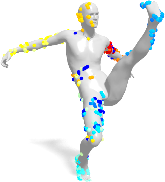
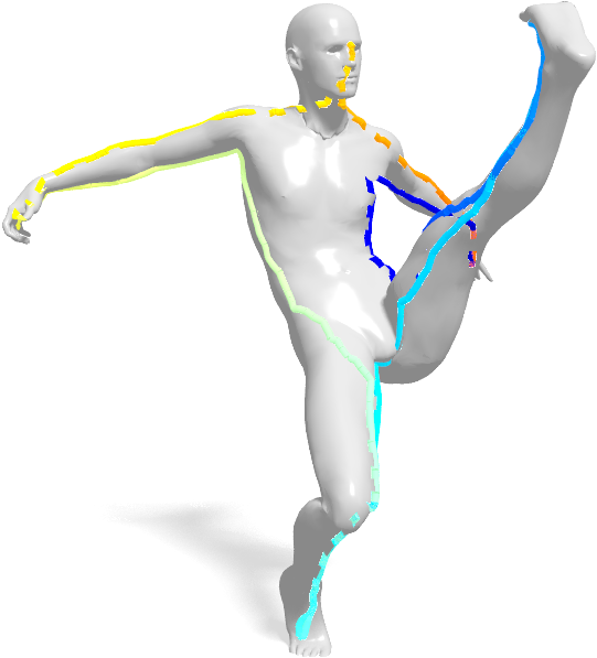
Figure 3: Matching between a 2D query shape (left) and a 3D target shape achieved by solving a LAP between the same point-wise features our method uses (middle) and our method (right).

Alternatively to the energy described here, one could also choose to enforce injectivity of $\varphi\colon M\to N$. This would lead to a linear assignment problem (LAP), which normally results in non-continuous matchings and is rather slow. If the shapes $M$ and $N$ are discretized at $m$ and $n$ points, respectively, the overall runtime of the Hungarian method munkres to solve this problem is $\mathcal{O}(n^{3})$. The method that we propose does not only provide for a smooth and continuous solution, but also has a better worst case runtime complexity than the LAP (cf. Theorem 3.1). Exploring the runtime of the LAP approach for one matching instance resulted in a runtime of 11 hours instead of just a few seconds for our method. The LAP matching result using the same features as in our experiments can be seen in Figure 3.

3.2 Optimization

So far we defined the energy we want to minimize. In the following, we address the discretization of this minimization problem and show that a globally optimal solution and an approximate solution within an arbitrary margin of the optimum can be computed efficiently by solving a shortest path problem on the discrete product manifold of both shapes. In practice, we often observed that many solutions with an energy close to the optimum are not qualitatively worse than the optimum. At the same time the algorithm finds solution close to the optimum very fast and spends a proportionally long time on finding the exact optimum. For this reason we implemented an approximate variation of our algorithm that uses an upper and lower bound to identify how close to the optimum the current solution is and stops if they are reasonably close.

To this end we assume that the 2D query shape $M$ and the 3D target shape $N$ are discretized. Thus, $M$ is given as a simple, directed circular graph, i.e., $\mathcal{G}_{M}=(\mathcal{V}_{M},\mathcal{E}_{M})$ with

$$\mathcal{V}_{M}= \{x_{0},\ldots,x_{m-1}\}\subset\mathbb{R}^{2}$$

$$\mathcal{E}_{M}= \{(x_{i},x_{j})\in\mathcal{V}_{M}^{2}~{}|~{}j\equiv i+1\mod{m}\}.$$

The target shape $N$ on the other hand is given as a 3D triangular mesh $\mathcal{G}_{N}=(\mathcal{V}_{N},\mathcal{E}_{N},\mathcal{F}_{N})$, where the set of vertices is denoted by $\mathcal{V}_{N}=\{y_{0},\ldots,y_{n-1}\}$ , $\mathcal{E}_{N}$ is the set of unoriented edges, and $\mathcal{F}_{N}$ the set of faces. Further, we assume that the feature maps $f_{M}\colon M\to\mathbb{R}^{k_{M}}$ and $f_{N}\colon N\to\mathbb{R}^{k_{N}}$ with a corresponding distance function are given as information on the vertices. Thus, we can represent the feature distance between all possible matches as a matrix $D\in\mathbb{R}^{m\times n}$ with $D_{ij}=\text{dist}(f_{M}(x_{i}),f_{N}(y_{j}))$ which can be precomputed.

Given this discretization, we define the product graph $\mathcal{G}_{M\times N}=(\mathcal{V}_{M\times N},\mathcal{E}_{M\times N},\mathcal{C}_{M\times N})$ via

$$\mathcal{V}_{M\times N}= \{0,\ldots,m-1\}\times\{0,\ldots,n-1\}$$

$$\mathcal{E}_{M\times N}= \left\{[({i_{0}},{j_{0}}),({i_{1}},{j_{1}})]\in\mathcal{V}_{M\times N}^{2}\right|$$

$$\quad({i_{1}}={i_{0}})\land(y_{j_{1}},y_{j_{0}})\in\mathcal{E}_{N}\text{ or }$$

$$\quad({i_{1}}={i_{0}}+1)\land({j_{1}}={j_{0}})\text{ or }$$

$$\quad({i_{1}}={i_{0}}+1)\land(y_{j_{1}},y_{j_{0}})\in\mathcal{E}_{N}\}$$

\begin{overpic}[trim=0.0pt 0.0pt 0.0pt -56.9055pt,clip,width=433.62pt]{images/product_manifold3} \put(25.0,75.0){$\mathcal{G}_{M\times N}$} \put(47.0,25.0){$L_{i}$} \put(17.0,25.0){$L_{i+1}$} \put(3.0,25.0){$L_{i+2}$} \put(48.0,45.0){$(i,j)$} \put(24.0,45.0){$(i+1,k)$} \put(34.0,16.0){$i$} \put(10.0,9.0){$\mathcal{G}_{M}$} \put(75.0,53.0){$j$} \put(70.0,30.0){$\mathcal{G}_{N}$} \end{overpic}

Figure 4: A node $(i,j)$ in the product graph $\mathcal{G}_{M\times N}$ represents a match between the vertex $i\in\mathcal{V}_{M}$ of the contour $M$ and the vertex $j\in\mathcal{V}_{N}$ of the surface $N$. All feasible matches with respect to vertex $i$ form the layer $L_{i}=\{i\}\times\mathcal{V}_{N}$. Edges are defined between a node $(i,j)$ and $(i+1,j)$ as well as $(i,k)$ and $(i+1,k)$ for all surface vertices $k\in\mathcal{V}_{N}$ that are adjacent to $j$. All these edges are directed and enforce a continuous matching.

The product graph takes the Cartesian product of the vertices in $\mathcal{G}_{M}$ and $\mathcal{G}_{N}$ representing all possible point-wise matchings between the two shapes and connects elements of this set iff their projections on the original shapes are connected (or identical). See Fig. 4 for an illustration. This preserves the original connectivity of each shape and enforces continuous solutions. Notice that the orientation of the circular 2D query shape is maintained because edges with $i_{0}\neq i_{1}$ are directed. Edges where $i_{0}=i_{1}$ are connected in both directions.

Furthermore, we will be interested in edge-wise instead of point-wise costs to solve the shortest path problem. We use the distances as stored in $D$ at each endpoint of one edge $\left[(i_{0},j_{0}),(i_{1},j_{1})\right]\in\mathcal{E}_{M\times N}$

$$D_{i_{0},j_{0}}= \ \text{dist}\left(f_{M}(x_{i_{0}}),f_{N}(y_{j_{0}})\right)$$

$$D_{i_{1},j_{1}}= \ \text{dist}\left(f_{M}(x_{i_{1}}),f_{N}(y_{j_{1}})\right)$$

and linearly interpolate the costs along the edge. This is equal to integrating over the average of both values and results in the cost function

$$\mathcal{C}_{M\times N}[({i_{0}} ,{j_{0}}),({i_{1}},{j_{1}})]=$$

$$\frac{D_{i_{0},j_{0}}+D_{i_{1},j_{1}}}{2}\cdot\left\|(x_{i_{0}},y_{j_{0}})-(x_{i_{1}},y_{j_{1}})\right\|.$$

$(x,y)$ is a 5D-coordinate with the stacked coordinate values from $x\in M$ (2D) and $y\in N$ (3D). This is a discretization of the line integral between both vertices from Equation 1.

To solve the shortest path problem a fixed source and target set is needed. We have no information about which vertices are contained in the solution but to have a circular path, we know that each $x\in M$ has to represented at least once in the solution. Therefore, the representation of the 2D shape $M$ is cut at an arbitrary $x$ and is extended by having two copies of $x_{0}$, namely at position $i=0$ and at position $i=m$. As a result, any continuous matching can be represented by a path from $(0,j)$ to $(m,j)$. Hence, an optimal matching can be cast as finding a shortest path in a graph if an initial match $(x_{0},y_{j})\in\Gamma_{\varphi}$ is given. Such a computation can easily be done by Dijkstra’s algorithm dijkstra59 . Using a priority heap the computation takes $\mathcal{O}(mn\cdot\log(mn))$ steps. Since there is no path from $(i_{1},j_{1})$ to $(i_{0},j_{0})$ if $i_{1}>i_{0}$, we associate to each layer $\{i\}\times\{0,\ldots,n-1\}$ a different priority heap and reduce the runtime to $\mathcal{O}(mn\log(n))$. These observations lead to the following theorem considering the above mentioned observations and the fact that we have to test $n$ different initial matches.

Theorem 3.1

Given a 2D query shape $M$ and a 3D target shape $N$, discretized by $m$ and $n$ vertices, respectively, we can find a minimizer of (1) in $\mathcal{O}(mn^{2}\log(n))$ steps. If $n=\mathcal{O}(m^{2})$, this leads to the subcubic runtime of $\mathcal{O}(n^{2.5}\log(n))$.

This theorem shows that we can find a globally optimal matching in polynomial time. Nonetheless, this may still lead to a high runtime since we have to find for each vertex $y\in\mathcal{V}_{N}$ a shortest path in $\mathcal{G}_{M\times N}$. In order to circumvent this problem we follow a branch-and-bound strategy inspired by the method of Appleton-2003 .

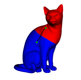
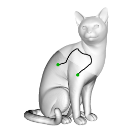
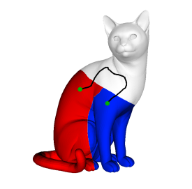
Figure 5: Exemplary first two iterations of the branch-and-bound algorithm. Paths are projected from the product manifold on the 3D shape. (Left) Absolute energy minimal path $p_{1}$ through the cut product manifold. (Middle Left) 3D Shape is separated in two subareas. One containing the source and the other the sink point of $p_{1}$. (Middle Right) In the next iteration one area is chosen; blue in this example but red will be processed later in the same way. The source and sink of the optimal path $p_{2}$ have to lie in the blue area. The rest of the path can go anywhere. This excludes the previous minimum $p_{1}$. (Right) If the source and sink of $p_{2}$ do not conincide, the blue area is again split in two.

$\mathcal{G}_{M\times N}=(\mathcal{V}_{M\times N},\mathcal{E}_{M\times N},\mathcal{C}_{M\times N})$, $\epsilon$

Matching path $\Gamma_{\varphi}$

Let $R:=\{0,\ldots,n-1\}$ ;

Define $\mathcal{R}=\{R\}$ and $b\colon\mathcal{R}\to\mathbb{R}$ via $b(R)=0$ ;

Define isFound=false ;

while isFound=false do

     

     lowerbound=$\min b$ ;

     Let $R\in\arg\min b$; $\mathcal{R}=\mathcal{R}\setminus\{R\}$ ;

     Find shortest path $\Gamma$ in $\mathcal{G}_{M\times N}$

      from $\{0\}\times R$ to $\{m\}\times R$ ;

     $\Gamma$ is a path from $(0,i)$ to $(m,j)$ ;

     if $i=j$ then

         isFound=true;$\Gamma_{\varphi}=\Gamma$

     else

         Find indices $l,k\in R$ with minimal Euclidean distance such that the shortest path

         in $\mathcal{G}_{M\times N}$ to $(m,k)$ originates in $(0,l)$ ;

         upperbound = $dist((0,k),(m,l))+dist((m,l),(m,k))$ in $\mathcal{G}_{M\times N}$ 

         if lowerbound $\geq(1-\epsilon)\cdot$ upperbound then

               $\Gamma_{\varphi}=dist((0,l),(m,l))$ ; break ;

         end if

              Divide $R$ into $R=R_{1}\cup R_{2}$ such that

                    $x\in R_{1}$:

              $\Leftrightarrow\text{dist}_{N}(x,i)<\text{dist}_{N}(x,j)$ ;

              Set $\mathcal{R}:=\mathcal{R}\cup\{R_{1},R_{2}\}$ ;

              Set $b(R_{1})=b(R_{2})=length(\Gamma)$ ;

              if $length(\Gamma)\leq\min b$ then

                   isFound=true ;

              end if

     end if

     end while

Algorithm 1 2D-to-3D matching via branch-and-bound. The blue code denotes the addition needed for the approximation algorithm.

The main idea is to follow a coarse-to-fine strategy. First we compute the shortest path between the sets $\{0\}\times R$ and $\{m\}\times R$, which connects $(0,i)$ with $(m,j)$. In the first iteration, we set $R=\mathcal{V}_{N}$. In this case $i$ and $j$ do not need to coincide but the energy of this path provides a lower bound on the optimal closed solution. If this path connects the corresponding points, i.e., $i=j$, we found a valid path. Otherwise, we separate the region $R$ into two sub-regions, $R_{1}$ containing $i$ and $R_{2}$ containing $j$, and recompute shortest paths starting and ending in $\{0\}\times R_{i}$ and $\{m\}\times R_{i}$ respectively. Since the shortest path of corresponding sub-regions will exclude the previously computed path, the optimal path in both $R_{1}$ and $R_{2}$ will have a larger energy than from the previously computed path. Thus, a natural order in which the subregions should be processed is induced. We propose to separate $R$ with respect to the geodesic distance $\text{dist}_{N}$ on the target shape $N$. We continue this process until we find our first matching path with $i=j$. Then, we still have to process those subdomains whose lower bound is smaller than the computed matching path. Afterwards, we are sure we found the globally optimal matching path $\Gamma_{\varphi}$. See Figure 5 for an illustration of one iteration.

Approximation. 

We observe that in practice already a few iterations in Algorithm 1 suffice if the features are distinctive and give a clear optimum. But in some cases, especially interclass matchings where the global optimum is not natural, the branch-and-bound is converging very slowy because many equally bad solutions exist. To circumvent this situation we implemented an extension using both an upper and lower bound of the optimal solution. If both are within a certain range of each other, the branch-and-bound stops. This guarantees a solution that is provably close to the optimum.

The lower bound comes, as in the previous section, from paths with $i\neq j$. The upper bound is obtained by choosing the open path in the current region whose endpoints $(0,i)$ and $(m,j)$ have the smallest Euclidean distance between $i$ and $j$. We then extend the path on the product manifold via Dijkstra to be a closed path. Because each closed path is a valid solution the energy of this path is an upper bound for the global optimum. Notice that there are no guarantees on the tightness of this upper bound. If the upper bound is within some chosen $\epsilon$ of the lower bound from the previous region (see global optimization) we know we are close to the global optimum and stop. The $\epsilon$ can indicate the absolute or relative error but we choose it as the relative one to be insensitive to the scale of the energies.

To keep the solution as close to the optimum as possible, we recompute the path between the $(0,i)$ and $(m,i)$ that closed the distance between the bounds. As a result from approximating the closing of the path from $(m,j)$, a different path between $(0,i)$ and $(m,i)$ might have a lower energy. We keep the starting point as the initial match and recompute the shortest path in the product manifold. Because we can compute the optimum with respect to a given starting point the energy of this path will be lower or equal to the energy of the upper bound.

4 Applications

In this section, we apply the proposed method to the problem of sketch-based deformable shape retrieval. We emphasize that our method is parameter-free, and the only choice is with respect to the 2D and 3D features $f_{M}(\cdot),f_{N}(\cdot)$ as well as the distance function $\text{dist}(\cdot,\cdot)$ between them. These choices depend on the specific application and help to illustrate the flexibility of our general 2D-to-3D shape matching approach.

4.1 Sketch-based shape retrieval

We consider a particular shape retrieval setting in which the dataset is assumed to be a collection of 3D shapes, and the query is a 2D silhouette (possibly drawn by a human) represented by a closed planar curve. Differently from previous techniques eitz2012sbsr ; furuya14 ; Li20151 ; su15mvcnn , our method does not use learning to compute features and most importantly, we allow the shapes to deform in a non-rigid fashion. The 2D-to-3D shape similarity is obtained by considering the minimal value of the energy $E(\varphi^{*})$ obtained by our optimization problem.

Datasets.

Due to the novelty of the application, to date there is no benchmark available for evaluating deformable 2D-to-3D shape retrieval methods. We therefore construct such a benchmark using the FAUST bogo14 , TOSCA bronstein08 and a subset of Non-rigid world bronstein2006nonrigid3d (additional poses for TOSCA, gorilla, lioness and seahorse) datasets. The FAUST dataset consists of 100 human shapes, subdivided into 10 classes (different individuals), each in 10 different poses. The latter two consist of over 100 shapes, subdivided into 12 classes (humans and animals in different poses). Shape sizes are fixed to around 7K (FAUST) and 10K (TOSCA) vertices.

In FAUST each class comes with a ‘null’ shape in a “neutral pose”, where no deformation has been applied, which we use to define the 2D queries. To this end we cut each null shape across a plane of symmetry and project the resulting boundary onto a plane. This gives rise to 2D queries of 200-400 points on average. Note that by doing so we retain the ground truth point-to-point mapping between the resulting 2D silhouette and the originating 3D target. This allows us to define a quantitative measure on the quality of the 2D-to-3D matching between objects of the same class. In the extended dataset, silhouettes of one shape showing all important extremities of the class are produced and the 2D query is extracted from the binary image. Hence, no point-to-point but only class ground truths are available. The same method can be applied to hand-drawn silhouetts.

As an addition to the queries produced through the actual 3D data, we drew a human by hand and used this as an additional query for the retrieval to show that the method also works on queries not produced using the targets. See Figure 6 for the sketch and query.

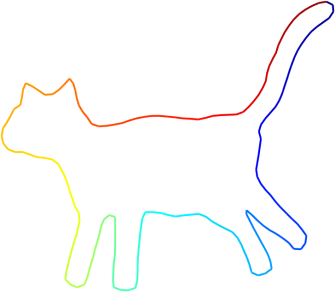
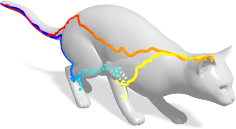
Figure 6: Handdrawn query for a cat shape and the extracted contour from the image. The image was simply thresholded to get a binary segmentation and then the contour extracted. Personal experience showed that drawing a solid silhouette is easier than directly drawing the contour. This also guarantees a shape as defined in Def. 1 without self-intersection or other degenerations.

Error measure.

Let $M$ be a 2D shape represented as a planar curve and $N$ a 3D shape represented as a surface. Let $\varphi\colon M\to N$ be a matching between a 2D query shape and a 3D target shape, and let $\varphi_{0}$ be the ground-truth matching. The matching error of $\varphi$ at point $x\in M$ is given by

$$\varepsilon_{\varphi}(x)=\frac{\text{dist}_{N}(\varphi(x),\varphi_{0}(x))}{diam(N)},$$ (6)

where $\text{dist}_{N}:N\times N\to\mathbb{R}^{+}_{0}$ denotes the geodesic distance on $N$ and $diam(N)=\max_{x,y\in N}\text{dist}_{N}(x,y)$ the geodesic diameter of $N$. Note that due to the normalization, the values of the error $\varepsilon$ are within $[0,1]$.

\begin{overpic}[trim=0.0pt 0.0pt 0.0pt 0.0pt,clip,width=433.62pt]{images/flatness} \put(4.0,1.0){\footnotesize(a) input 2D} \put(36.5,1.0){\footnotesize(b)} \put(65.0,1.0){\footnotesize(c)} \put(82.0,1.0){\footnotesize(d) input 3D} \put(49.4,25.0){\footnotesize isometric} \put(53.6,22.0){\footnotesize$\approx$} \end{overpic}

Figure 7: Spectral features are constructed by considering the query shape (a) as the boundary of a 2D region (b), which is assumed to be a near-isometric deformation of a sub-region (c) of the 3D target shape (d). The 2D tessellation (b) is obtained via shewchuk02 .

Spectral features.

In this chapter we advocate the adoption of spectral quantities to define compatible features between 2D and 3D shapes. Note that differently from existing methods for 2D-to-3D matching, we compute local features independently for each given pair of shapes, i.e., no cross-modal metric learning is carried out.

Let $\Delta_{N}$ be the symmetric Laplace-Beltrami operator on the 3D shape $N$. $\Delta_{N}$ admits an eigendecomposition with non-negative eigenvalues $0=\lambda_{0}<\lambda_{1}\leq\dots$ and corresponding orthogonal eigenfunctions $\psi_{j}\colon N\to\mathbb{R}$ such that $\Delta_{N}\psi_{j}=\lambda_{j}\psi_{j}$. For the definition of our feature maps, we consider multi-dimensional spectral descriptors, i.e., features constructed as functions of $\lambda_{j}$ and $\psi_{j}$. Note that, since $\Delta_{N}$ is invariant to isometric transformations of $N$, the derived spectral descriptors also inherit this invariance.

Popular spectral features are the scaled Heat Kernel Signature (HKS) sun09 and the Wave Kernel Signature (WKS) aubry11 ,

$$f^{\mathrm{HKS}}_{k}(x) =\sum_{j\geq 1}e^{-t_{k}\lambda_{j}}\psi^{2}_{j}(x),$$ (7)

$$f^{\mathrm{WKS}}_{k}(x) =\sum_{j\geq 1}e^{-\frac{(\log e_{k}-\log\lambda_{j})^{2}}{2\sigma^{2}}}\psi^{2}_{j}(x),$$ (8)

where $k=1,\ldots,d$ are the dimensions of the descriptors describing. In our experiments, we used $d=100$ and the parameters $t_{1},\ldots,t_{d}$ of HKS and $e_{1},\ldots,e_{d},\sigma$ of WKS were taken as suggested by the respective authors. All descriptors were normalized to have maximum value 1 in order to improve their robustness.

For the 2D case, designing features that can be compared to their 3D counterparts can be a challenging task. The difficulty is exacerbated here because the shapes are allowed to deform. To this end, we consider the solid $U$ of $M$, i.e., $\partial U=M$ (cf. Definition 1). In other words, we model the 2D query as a flat 2-manifold with boundary. This new manifold can be regarded as a nearly isometric transformation (due to flatness and possibly a change in pose) of a portion of the full 3D target (see Fig. 7). Taking this perspective allows us to leverage some recent advances in partial 3D matching rodola15 , namely that partiality transformations of a surface preserve the Laplacian eigenvalues and eigenfunctions, up to some bounded perturbation.

An implication of this is that we can still compute spectral descriptors on the flat solid $U$ and expect them to be comparable with those on the full 3D target. By doing so, we make the assumption that $U$ can be approximated as a part of nearly-isometrically deformed $M$ for the features to be comparable. We then define the feature maps $f^{\text{HKS}}_{M},f^{\text{WKS}}_{M}\colon M\to\mathbb{R}^{d}$ on $M$ by restricting the descriptors computed on $U$ to its boundary curve $\partial U=M$ (see Fig. 8, top row). In other words, we have the spectral features $f_{M}=f_{U}|_{M}$ for the query shape $M$.

\begin{overpic}[trim=0.0pt 0.0pt 0.0pt 0.0pt,clip,width=86.72267pt]{images/3ddescr_arrow} \end{overpic}

\begin{overpic}[trim=0.0pt 0.0pt 0.0pt 0.0pt,clip,width=108.405pt]{images/2ddescr} \end{overpic}

\begin{overpic}[trim=0.0pt 0.0pt 0.0pt 0.0pt,clip,width=108.405pt]{images/sketchdescr} \end{overpic}

\begin{overpic}[trim=0.0pt 0.0pt 0.0pt 0.0pt,clip,width=86.72267pt]{images/3dseg} \put(12.0,1.0){\footnotesize input 3D} \end{overpic}

\begin{overpic}[trim=0.0pt 0.0pt 0.0pt 0.0pt,clip,width=108.405pt]{images/2dseg} \put(4.0,1.0){\footnotesize input 2D, tessellated} \end{overpic}

\begin{overpic}[trim=0.0pt 0.0pt 0.0pt 0.0pt,clip,width=108.405pt]{images/sketchseg} \put(20.0,1.0){\footnotesize input 2D} \end{overpic}

Figure 8: Computation of local features for elastic matching. Top: $L_{1}$-distance (blue to red) between spectral 3D descriptors of a reference point (white dot) and 3D descriptors computed on the remaining shape (left) as well as 2D descriptors on the tessellated query solid (middle). Bottom: Consensus regions detected in 3D and 2D using rodola-cgf14 . The restricted features (right) are used in the energy (1) to drive the matching process.

Segment features.

As an additional ‘coarse’ feature we use corresponding regions on the 2D query and the 3D shape. Based on the previous observations, we are able to automatically extract compatible regions on the two objects (namely on $U$ and $N$) by consensus segmentation rodola-cgf14 , a deformation-invariant region detection technique which directly operates with the Laplace-Beltrami eigenfunctions of a given shape. The region detection step on the two shapes is performed independently; we then obtain the 2D-to-3D region mapping by solving a simple linear assignment problem via the Hungarian algorithm munkres . Note that this assignment problem is typically very small. Assuming we have $r$ regions per shape (usually in the range of 5 to 10), the final result of this procedure is a pair of corresponding labelings $f_{M}^{\mathrm{SEG}}:M\to\mathbb{N}^{r}$ and $f_{N}^{\mathrm{SEG}}:N\to\mathbb{N}^{r}$ (see Fig. 8, bottom row).

Distance function.

The final feature maps are obtained by simple concatenation, namely $f:=(f^{\mathrm{HKS}},f^{\mathrm{WKS}},f^{\mathrm{SEG}})$. In order to compare the feature maps on $M$ and $N$, we define the distance function:

$$\mathrm{dist}(f_{M}(x),f_{N}(y)) = \|f_{M}^{\mathrm{HKS}}(x)-f_{N}^{\mathrm{HKS}}(y)\|_{1}$$

$$+ \|f_{M}^{\mathrm{WKS}}(x)-f_{N}^{\mathrm{WKS}}(y)\|_{1}$$

if ${f_{M}^{\text{SEG}}(x)=f_{N}^{\text{SEG}}(y)}$, and set ${\text{dist}(f_{M}(x),f_{N}(y))=\tau}$ otherwise. Here, $\tau>0$ is a positive value larger than any other values in the feature matrix to prevent matching points belonging to different regions. In our experiments, we used $\tau=10^{3}$.

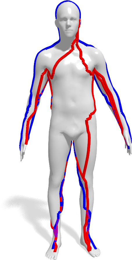
Figure 9: Sensitivity of the spectral features to increasing number of eigenfunctions. On the right we show typical solutions obtained when using 25 (blue) and 200 (red) eigenfunctions. See Eq. (6) for details on the error curve.

4.2 Sensitivity analysis

In most shape analysis applications, only the first $k$ eigenfunctions of $\Delta$ are used to define $f^{\mathrm{WKS}}$ and $f^{\mathrm{HKS}}$. In the classical 3D-to-3D setting, for large $k$ the resulting descriptors tend to be more accurate, but at the same time become more sensitive to the lack of isometry relating the two shapes. We performed a sensitivity analysis of our elastic matching method on a subset of our FAUST-derived dataset to determine the optimal number of eigenfunctions.

We observed a similar trend to the 3D-to-3D case in our 2D-to-3D setting where naturally the isometry is only approximate giving better results for a low $k$, as reported in Fig. 9. From this analysis we selected $k=25$ as the fixed number of eigenfunctions for all subsequent experiments. In the figure, we plot cumulative curves showing the percent of matches with a geodesic error smaller than a variable threshold (see Eq. (6)).

4.3 Runtime

We implemented our method in C++ and ran it on an Intel Core i7 3.4GHz CPU. In Fig. 10 we show the execution times of our method on the FAUST dataset (10 queries and 100 targets). The plotted results show that for 3D shapes of fixed size, in practice the runtime grows linearly with the number of 2D query points $m$ and quadratic with the number of points on the 3D target $n$.

Fig. 11 shows the decrease of the average runtime with growing parameter $\epsilon$ for the approximation algorithm. The plot shows that after decreasing rapidly over $\epsilon\approx 0.05$ the runtime stays relatively constant with no chang in the MAP. Therefore, choosing a small $\epsilon$ leads to a good quality-runtime ratio.

\begin{overpic}[trim=56.9055pt 28.45274pt 128.0374pt 28.45274pt,clip,width=195.12767pt]{images/runtimes} \end{overpic}

\begin{overpic}[trim=56.9055pt 28.45274pt 128.0374pt 28.45274pt,clip,width=195.12767pt]{images/runtimes_n} \end{overpic}

Figure 10: Blue: Mean runtime with standard deviation shaded. Red: Optimal curve of form $a\cdot x^{b}$ fitted to the data. Left: Runtime of our matching method on 3D targets with $\sim$7k vertices (FAUST dataset). On the $x$ axis we vary the size of the 2D query from 25 to 400 points. The fitted curve has $a=0.0245$ and $b=1.1518$ so the real runtime is nearly linear in $m$. Right: Runtime with a $100$ vertex query and upsampled FAUST shapes. On the $x$ axis we vary the size of the 3D targets from 7k to 24k. The fitted curve has $a=2.6466\cdot 10^{-7}$ and $b=2.1147$ making the real runtime nearly quadratic in $n$ with a really small constant.

4.4 Sketch-based shape retrieval

We retrieve the most fitting element from a collection of 3D shapes in comparison to the query 2D silhouette. The matching energy $E(\varphi^{*})$ obtained by our optimization problem is a suitable measurement for shape similarity and we match the query to every instance of the collection, choosing the one with lowest energy as the result.

We evaluated the performance of our retrieval pipeline on the extended 2D-to-3D TOSCA dataset. As baselines for our comparisons we use the spectral retrieval method of reuter06 and a pure region-based retrieval technique using segments computed with rodola-cgf14 ; both are the foundation for the features we use. The rationale of these experiments is to show that these features are not sufficient to guarantee good retrieval performance. However, using these quantities in our elastic matching pipeline enables promising results even in challenging cases. The first baseline method we compare against is Shape-DNA reuter06 using the (truncated) spectrum of the Laplace-Beltrami operator as a global isometry-invariant shape descriptor. We apply this method to compare targets in the 3D database with flat tessellations of the 2D queries. The second method used in the comparisons is a simple evaluation of the matching cost obtained when putting the consensus regions into correspondence via linear assignment (see Fig. 8). Since this step typically produces good coarse 2D-to-3D matchings, it can be used as a retrieval procedure per se.

\begin{overpic}[trim=108.12054pt 14.22636pt 48.36958pt 45.52458pt,clip,width=216.81pt]{images/eps} \end{overpic}

Figure 11: The average runtime of the TOSCA dataset with values between $0$ (globally optimal) and $0.3$ (within 30% of the optimum). The runtime nearly stagnates after $\epsilon=0.05$ (only one or two iterations) but small $\epsilon$ already lead to significant improvement in the runtime and comparable results (as shown in Table 1). The segmentation feature was not used.

We test the global optimization using all features we presented before. For the approximate optimization we use all features except the segment features. The reason is we noticed that the energies without the segments are comparable for same-class matching; the only difference being the matchings only take place on one symmetric half of the 3D shape (see Fig. 12). Although this is not the favored solution, since it does not substantially change the energy, it is suitable for retrieval. Unfortunately, without the coarse matching of the segments the globally optimal solution for interclass matchings can take longer to converge because there are many equally best solutions - still with a high energy in comparison. Therefore, we use the segment features for the globally optimal method but show that we can get similar results without this feature and the approximate method.

The results of the shape retrieval experiments are reported in Table 1. $\epsilon=0.001$ was used for the approximation experiments. We used average precision (AP) and mean average precision (MAP) as measures of retrieval performance. The results slightly differ from the ones reported in LRSBC16 due to a small bug in the code. Additional qualitative examples of solutions obtained with our method are shown in Fig. 13. Fig. 12 shows an embedding and clustering of all 3D models using the matching energies (with the approximation algorithm).

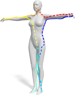
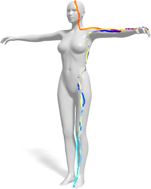
Figure 12: (Left and Middle) Example of the same query matched to the same shape, once using the segmentation features (left) and once without (right). Dashed lines indicate a path on the backside normally not visible in this perspective. The matchings are very similar but without segments the path only considers one of the symmetric sides (normally because it is slightly shorter). (Right) 2-dimensional embedding of all 3D models using the approximate matching energies to each of the $k$ sketches as $k$-dimensional coordinates for each model. Except for one outlier (horse close to the centaurs), all classes are perfectly separable.

	Global (Ours)	Approximation (Ours)	Shape DNA	Consensus Segmentation
cat	1.0000	1.0000	0.2852	0.2518
dog	1.0000	0.9615	0.3519	0.3970
horse	0.9987	0.9313	0.4469	0.3432
human	1.0000	1.0000	0.7447	0.9985
lioness	0.9984	0.9587	0.7022	0.5419
seahorse	1.0000	1.0000	0.0779	1.0000
wolf	1.0000	0.8082	0.2230	0.2470
human (hd)	1.0000	1.0000	0.7096	0.9462
cat (hd)	0.9888	0.9772	0.8622	-
MAP	0.9984	0.9597	0.4720	0.5907

Table 1: Retrieval results on the 2D-to-3D extended dataset. For each method we show per-class AP and, in the last row, the MAP. The global algorithm uses all features and the approximation does not use the segmentation. $\epsilon$ was chosen to be $0.001$. hd refers to handdrawn sketches. Shape DNA refers to reuter06 and Consensus Segmentation to rodola-cgf14 .

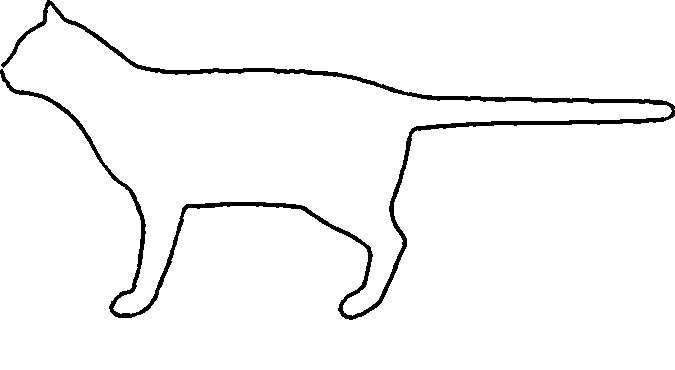
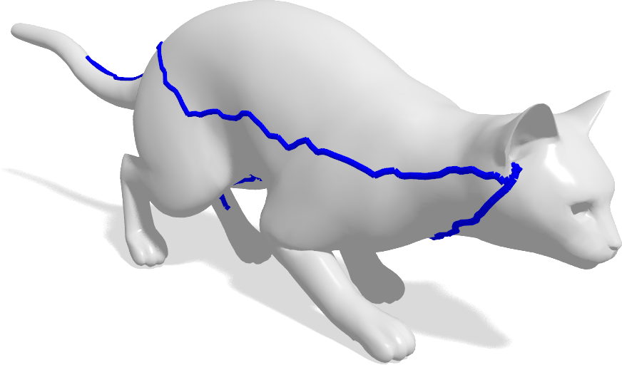
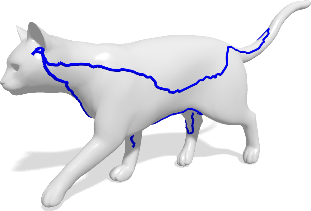
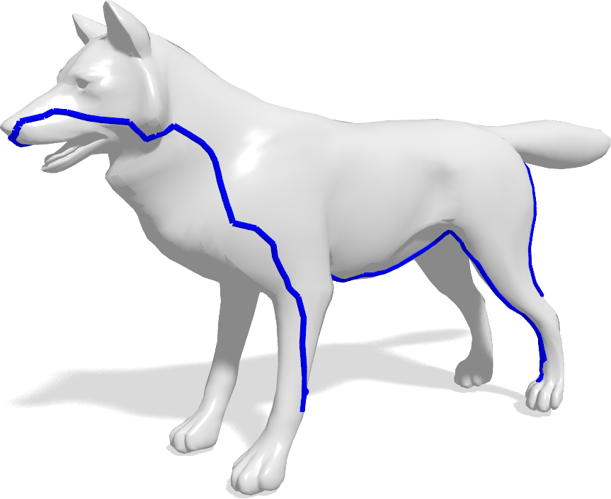
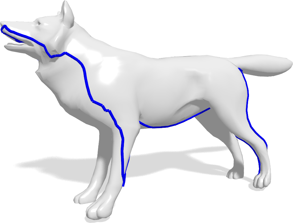
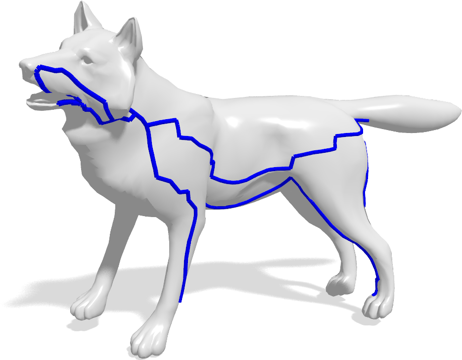
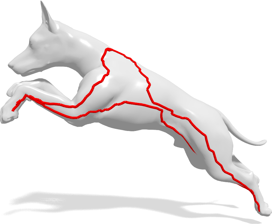
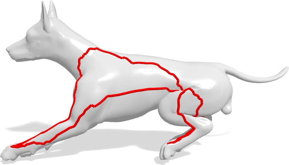
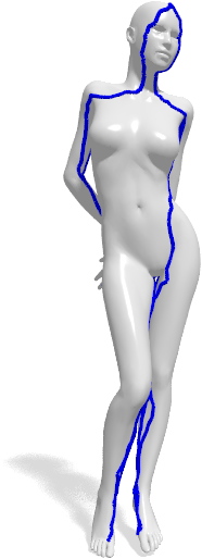
Figure 13: Retrieval examples on the TOSCA dataset. Left: Two of the three 2D queries (cat and wolf) have missing parts (two legs in contrast to Fig. 2). Each row shows the top 5 results (ranked by matching energy) provided by our method. The corresponding matching curves are shown on top of the 3D targets. Note that the dataset only contains 3 wolf shapes, which show up as the top 3 matches. The next matches are shapes of the class “dog”, which is a semantically similar class.

5 Conclusion

We proposed a polynomial-time solution for matching deformable planar curves to 3D shapes. We prove that the worst-case complexity of this algorithm is $\mathcal{O}(mn^{2}\log(n))$, where $m$ and $n$ denote the number of samples on the query curve and the 3D shape respectively. We show experimentally that the runtime remains linear with respect to $m$, even when employing a branch-and-bound strategy, making this a very efficient approach that matches queries with hundreds of vertices to 3D shapes with ten thousands of vertices in a few seconds. Our algorithm can compute the globally optimal or a $\epsilon$-tight solution. The approximate method is more efficient if the features are not discrimative enough which causes many iterations in the branch-and-bound strategy.

Our algorithm provides a powerful tool for shape analysis, and in particular has great potential in applications such as 3D shape retrieval from 2D sketches.

Limitations.

The main limitation of our method is the assumption that the query 2D shape is a closed planar curve. In some situations, this may limit the ‘expressivity’ of the sketch and pose a disadvantage compared to image-based approaches in sketch-based retrieval applications. Furthermore, due to the shortest-path computation the algorithm favors solutions having a shorter length on the 3D target shape which are not semantically perfect. This makes the correspondence not suitable as input for further applications.

Future research directions.

One notable drawback of our discrete optimization is the use of Dijkstra’s algorithm for finding shortest paths on the product manifold, which in some situations may not be a consistent discretization of the geodesic distance. In follow-up works, we will explore the use of consistent fast-marching-like schemes.

- [1] Ben Appleton and Changming Sun. Circular shortest paths by branch and bound. Pattern Recognition, 36(11):2513–2520, 2003.
- [2] M. Aubry, U. Schlickewei, and D. Cremers. The wave kernel signature: A quantum mechanical approach to shape analysis. In Proc. ICCV, pages 1626–1633, 2011.
- [3] Federica Bogo, Javier Romero, Matthew Loper, and Michael J. Black. FAUST: Dataset and evaluation for 3D mesh registration. In Proc. CVPR, June 2014.
- [4] A. Bronstein, M. Bronstein, L. Guibas, and M. Ovsjanikov. Shape Google: Geometric words and expressions for invariant shape retrieval. Trans. Graphics, 30(1), 2011.
- [5] Alexander Bronstein, Michael Bronstein, and Ron Kimmel. Numerical Geometry of Non-Rigid Shapes. Springer, 2008.
- [6] Alexander M. Bronstein, Michael M. Bronstein, and Ron Kimmel. Efficient computation of isometry-invariant distances between surfaces. SIAM J. Scientific Computing, 28/5:1812–1836, 2006.
- [7] Alexander M Bronstein, Michael M Bronstein, and Ron Kimmel. Generalized multidimensional scaling: a framework for isometry-invariant partial surface matching. PNAS, 103(5):1168–1172, 2006.
- [8] Edsger W. Dijkstra. A note on two problems in connexion with graphs. Numerische Mathematik, 1:269–271, 1959.
- [9] Mathias Eitz, Ronald Richter, Tamy Boubekeur, Kristian Hildebrand, and Marc Alexa. Sketch-based shape retrieval. Trans. Graphics, 31(4):1–10, 2012.
- [10] Thomas Funkhouser, Patrick Min, Michael Kazhdan, Joyce Chen, Alex Halderman, David Dobkin, and David Jacobs. A search engine for 3D models. Trans. Graphics, 22(1):83–105, 2003.
- [11] Takahiko Furuya and Ryutarou Ohbuchi. Hashing cross-modal manifold for scalable sketch-based 3D model retrieval. In Proc. 3DV, 2014.
- [12] Yulia Gryaditskaya, Felix Hähnlein, Chenxi Liu, Alla Sheffer, and Adrien Bousseau. Lifting freehand concept sketches into 3d. ACM Transactions on Graphics (Proc. SIGGRAPH Asia), 39, 12 2020.
- [13] Robert Herzog, Daniel Mewes, Michael Wand, Leonidas Guibas, and Hans-Peter Seidel. LeSSS: Learned shared semantic spaces for relating multi-modal representations of 3D shapes. Computer Graphics Forum, 34(5):141–151, 2015.
- [14] Moos Hueting, Maks Ovsjanikov, and Niloy J Mitra. CrossLink: joint understanding of image and 3D model collections through shape and camera pose variations. Trans. Graphics, 34(6):233, 2015.
- [15] Artiom Kovnatsky, Michael M. Bronstein, Xavier Bresson, and Pierre Vandergheynst. Functional correspondence by matrix completion. In Proc. CVPR, 2015.
- [16] Zorah Lähner, Emanuele Rodolà, Frank R. Schmidt, Michael M. Bronstein, and Daniel Cremers. Efficient globally optimal 2d-to-3d deformable shape matching. In Proc. of IEEE Conference on Computer Vision and Pattern Recognition (CVPR), 2016.
- [17] Marius Leordeanu and Martial Hebert. A spectral technique for correspondence problems using pairwise constraints. In Proc. ICCV, 2005.
- [18] Bo Li, Yijuan Lu, Chunyuan Li, et al. A comparison of 3D shape retrieval methods based on a large-scale benchmark supporting multimodal queries. CVIU, 131:1 – 27, 2015.
- [19] M. Maes. Polygonal shape recognition using string-matching techniques. Pattern Recognition, 24(5):433–440, 1991.
- [20] Facundo Mémoli and Guillermo Sapiro. A theoretical and computational framework for isometry invariant recognition of point cloud data. Foundations of Computational Mathematics, 5(3):313–347, 2005.
- [21] James Munkres. Algorithms for the assignment and transportation problems. J. SIAM, 5(1):32–38, 1957.
- [22] Weizhi Nie, Yue Zhao, Jie Niea, An-An Liu, and Sicheng Zhaob. Cln: Cross-domain learning network for 2d image-based 3d shape retrieval. IEEE Transactions on Circuits and Systems for Video Technology, 2021.
- [23] Maks Ovsjanikov, Mirela Ben-Chen, Justin Solomon, Adrian Butscher, and Leonidas Guibas. Functional maps: A flexible representation of maps between shapes. Trans. Graphics, 31(4):1–11, July 2012.
- [24] Jonathan Pokrass, Alexander M Bronstein, Michael M Bronstein, Pablo Sprechmann, and Guillermo Sapiro. Sparse modeling of intrinsic correspondences. Computer Graphics Forum, 32(2):459–468, 2013.
- [25] Martin Reuter, Franz-Erich Wolter, and Niklas Peinecke. Laplace-Beltrami spectra as ’shape-DNA’ of surfaces and solids. Comput. Aided Design, 38(4):342–366, April 2006.
- [26] E. Rodolà, A.M. Bronstein, A. Albarelli, F. Bergamasco, and A. Torsello. A game-theoretic approach to deformable shape matching. In Proc. CVPR, 2012.
- [27] E. Rodolà, S. Rota Bulò, T. Windheuser, M. Vestner, and D. Cremers. Dense non-rigid shape correspondence using random forests. In Proc. CVPR, 2014.
- [28] E. Rodolà, L. Cosmo, M. M. Bronstein, A. Torsello, and D. Cremers. Partial functional correspondence. Computer Graphics Forum, 2016.
- [29] E. Rodolà, S. Rota Bulò, and D. Cremers. Robust region detection via consensus segmentation of deformable shapes. Computer Graphics Forum, 33(5):97–106, 2014.
- [30] E. Rodolà, A. Torsello, T. Harada, Y. Kuniyoshi, and D. Cremers. Elastic net constraints for shape matching. In Proc. ICCV, 2013.
- [31] F. R. Schmidt, D. Farin, and D. Cremers. Fast matching of planar shapes in sub-cubic runtime. In Proc. ICCV, 2007.
- [32] F. R. Schmidt, E. Töppe, and D. Cremers. Efficient planar graph cuts with applications in computer vision. In Proc. CVPR, June 2009.
- [33] T. Schoenemann and D. Cremers. A combinatorial solution for model-based image segmentation and real-time tracking. Trans. PAMI, 32(7):1153–1164, 2010.
- [34] Jonathan Richard Shewchuk. Delaunay refinement algorithms for triangular mesh generation. Comput. Geom. Theory Appl., 22(1-3):21–74, 2002.
- [35] Hang Su, Subhransu Maji, Evangelos Kalogerakis, and Erik G. Learned-Miller. Multi-view convolutional neural networks for 3D shape recognition. In Proc. ICCV, 2015.
- [36] Jian Sun, Maks Ovsjanikov, and Leonidas Guibas. A concise and provably informative multi-scale signature based on heat diffusion. In Proc. SGP, pages 1383–1392, 2009.
- [37] Hedi Tabia and Hamid Laga. Learning shape retrieval from different modalities. Neurocomputing, 253:24–33, 2017.
- [38] Johan WH Tangelder and Remco C Veltkamp. A survey of content based 3D shape retrieval methods. Multimedia Tools and Applications, 39(3):441–471, 2008.
- [39] Oliver Van Kaick, Hao Zhang, Ghassan Hamarneh, and Daniel Cohen-Or. A survey on shape correspondence. Computer Graphics Forum, 30(6):1681–1707, 2011.
- [40] Lingjing Wang, Cheng Qian, Jifei Wang, and Yi Fang. Unsupervised learning of 3d model reconstruction from hand-drawn sketches. Association for Computing Machinery, 2018.
- [41] T. Windheuser, U. Schlickewei, F. R. Schmidt, and D. Cremers. Geometrically consistent elastic matching of 3D shapes: A linear programming solution. In Proc. ICCV, 2011.
- [42] Cheng Xu, Zhaoqun Li, Qiang Qiu, Biao Leng, and Jingfei Jiang. Enhancing 2d representation via adjacent views for 3d shape retrieval. In Proceedings of the IEEE/CVF International Conference on Computer Vision (ICCV), October 2019.
- [43] Song Yang. Sketch-based 3d shape retrieval with multi-silhouette view based on convolutional neural networks. In 2020 13th International Conference on Intelligent Computation Technology and Automation (ICICTA), pages 223–226, 2020.
- [44] Yan Zhou and Fanzhi Zeng. 2d compressive sensing and multi-feature fusion for effective 3d shape retrieval. Information Sciences, 409-410:101–120, 2017.