The 5 – 10 $\rm{ke}$V AGN luminosity function at 0.01¡z¡4.0

The active galactic nuclei X-ray luminosity function traces actively accreting supermassive black holes and is essential for the study of the properties of the active galactic nuclei (AGN) population, black hole evolution, and galaxy-black hole coevolution. Up to now, the AGN luminosity function has been estimated several times in soft ($\rm{0.5-2\,keV}$) and hard X-rays ($\rm{2-10\,keV}$). AGN selection in these energy ranges often suffers from identification and redshift incompleteness and, at the same time, photoelectric absorption can obscure a significant amount of the X-ray radiation. We estimate the evolution of the luminosity function in the $\rm{5-10\,keV}$ band, where we effectively avoid the absorbed part of the spectrum, rendering absorption corrections unnecessary up to $\rm{N_{H}{\sim}10^{23}cm^{-2}}$. Our dataset is a compilation of six wide, and deep fields: MAXI, HBSS, XMM-COSMOS, Lockman Hole, XMM-CDFS, AEGIS-XD, Chandra-COSMOS, and Chandra-CDFS. This extensive sample of ${\sim}1110$ AGN ($\rm{0.01<z<4.0}$, $\rm{41<\log L_{x}<46}$) is 98% redshift complete with 68% spectroscopic redshifts. For sources lacking a spectroscopic redshift estimation we use the probability distribution function of photometric redshift estimation specifically tuned for AGN, and a flat probability distribution function for sources with no redshift information. We use Bayesian analysis to select the best parametric model from simple pure luminosity and pure density evolution to more complicated luminosity and density evolution and luminosity-dependent density evolution. We estimate the model parameters that describe best our dataset separately for each survey and for the combined sample. We show that, according to Bayesian model selection, the preferred model for our dataset is the luminosity-dependent density evolution (LDDE). Our estimation of the AGN luminosity function does not require any assumption on the AGN absorption and is in good agreement with previous works in the $\rm{2-10\,keV}$ energy band based on X-ray hardness ratios to model the absorption in AGN up to redshift three. Our sample does not show evidence of a rapid decline of the AGN luminosity function up to redshift four.

1 Introduction

The X-ray luminosity function (XLF) of active galactic nuclei (AGN) and its evolution provides a view of black hole (BH) growth across cosmic time. Several studies use the XLF to constrain models of BH evolution through simulations and semi-analytic models (e.g., Mahmood et al. 2005; Hopkins et al. 2005; Hirschmann et al. 2012, 2014; Enoki et al. 2014) and to investigate the possible galaxy-BH coevolution (e.g., Hopkins et al. 2007; Marulli et al. 2008; Zheng et al. 2009; Fanidakis et al. 2011). The XLF is also used to constrain the properties of the AGN population, for example, by creating population synthesis models that describe the cosmic X-ray background (CXB) and thus inferring the fraction of Compton-thick AGN (e.g., Gilli et al. 2007; Treister et al. 2009; Draper & Ballantyne 2009; Akylas et al. 2012). Additionally, the XLF is used to test the still open question of AGN triggering: mergers vs secular processes (Draper & Ballantyne 2012). The multivariate changes of the AGN phase can be studied by combining the XLF with luminosity functions in other wavelengths (e.g., Han et al. 2012; Hopkins et al. 2005). For example, the connection between X-ray and infrared radiation from AGN has been studied by means of reconciling the CXB with the infrared background through the corresponding luminosity functions (Ballantyne & Papovich 2007).

Early X-ray surveys showed that the space density of AGN follows a broken power-law distribution and it was proposed that the XLF only evolves with redshift in luminosity (pure luminosity evolution, hereafter PLE; Maccacaro et al. 1983, 1984), while subsequent studies showed that the evolution stops, or dramatically slows down after a critical redshift value (e.g. Boyle et al. 1994; Page et al. 1996; Jones et al. 1997). Recent works in the soft X-ray regime ($\rm{0.5-2\,keV}$) support a luminosity-dependent density evolution (LDDE) over the simple PLE with the number density of AGN peaking in redshift $\rm{z=1-2}$ (Miyaji et al. 2000; Hasinger et al. 2005; Ebrero et al. 2009). Similarly in the hard X-ray band ($\rm{2-10\,keV}$) several works support LDDE over PLE (Ueda et al. 2003; La Franca et al. 2005; Ebrero et al. 2009; Ueda et al. 2014; Miyaji et al. 2015). Other studies at the same energy band also tested simultaneous variations in luminosity and density with different parametrization, namely, independent luminosity and density evolution (ILDE; Yencho et al. 2009) and luminosity and density evolution (LADE; Aird et al. 2010).

According to the unified model of AGN (Antonucci 1993; Urry & Padovani 1995), a supermassive black hole is found at the center of each AGN, surrounded by an accretion disk and a torus of gas and dust. The current accepted view of the radiation mechanism includes X-ray production in the vicinity of the black hole through Comptonization of disk photons in a population of hot thermal electrons (Haardt & Maraschi 1993). The torus is responsible for the obscuration of X-rays due to photoelectric absorption. The torus also generates infrared emission, which is optical radiation reprocessed by the dust. For the luminosity function in the X-ray energy ranges $\rm{0.5-2\,keV}$ and $\rm{2-10\,keV,}$ a correction factor must be applied depending on the absorption power of the obscuring torus in each source. This absorption power is either calculated from the spectrum or roughly estimated from the observed flux in at least two X-ray energy bands. An additional correction factor is often applied to take redshift incompleteness into account in the sample under investigation.

In this work, we study X-ray emission in a hard band ($\rm{5-10\,keV}$), avoiding the absorbed part of the spectrum. Previous works over the same energy range attempted to put constraints on the bright end of the $\rm{5-10\,keV}$ XLF. La Franca et al. (2002) used ${\sim}160$ AGN detected in BeppoSAX, ASCA, and HEAO 1 with a flux limit of $\rm{F_{x}=3\times 10^{-14}erg\,s^{-1}}\,cm^{-2}$, while Ebrero et al. (2009) used a sample of ${\sim}120$ XMM detected AGN with a flux limit of $\rm{F_{x}=6.8\times 10^{-15}erg\,s^{-1}}\,cm^{-2}$. The small number of available AGN was not enough to differentiate between PLE and LDDE models and the authors resorted to fixing the evolutionary parameters of the luminosity function. Similarly, efforts have been made to determine the X-ray luminosity function at energies higher than $\rm{10\,keV}$ using objects detected with INTEGRAL and SWIFT-BAT (Beckmann et al. 2006; Sazonov et al. 2007; Paltani et al. 2008; Burlon et al. 2011). These samples include very bright local objects (z¡0.1), which put constraints on the local luminosity function, but are not able to constrain the evolution of the AGN number density with redshift.

With the combination of recent multiwavelength surveys, we are able to create a sizable sample of ${\sim}1100$ sources with a flux limit of about $\rm{F_{x}=1.5\times 10^{-16}erg\,s^{-1}\,cm^{-2}}$, which is 10 times deeper and 5-6 times more numerous than previously available samples in the same energy range. Spectroscopic redshifts (spec-z), combined with accurate photometric redshifts (photo-z), provide a 98% redshift complete sample that is ideal for probing AGN evolution. We determine the XLF and its evolution in the $\rm{5-10\,keV}$ band testing the evolutionary models used in the literature. We perform Bayesian analysis to investigate in detail the probability distribution function for each parameter that describes the luminosity function, per survey and in the combined sample. This approach provides an accurate view of the parameters without assuming Gaussian distribution around the best value. In §2.1 we present the surveys used for this work, and in §2.2 we discuss the selection of the $\rm{5-10\,keV}$ energy range. In §3 we describe the models we used in estimating the luminosity function. In §4 we describe our analysis and the selection of the best model for our dataset. In §5 we discuss the LDDE model, compare the information contained in each survey separately, and predict the expected number of AGN for future surveys. We adopt the cosmological parameters ${{\Omega}_{\Lambda}=0.7}$, ${{\Omega}_{m}=0.3}$, and $\rm{H_{0}=70\,kms^{-1}Mpc^{-1}}$.

2 Dataset definition

We combined wide/medium angle surveys (MAXI, HBSS, COSMOS) with pencil beam X-ray fields (Lockman Hole (LH), AEGIS, CDFS) to create a sample of $\rm{5-10\,keV}$ detected AGN. We exclude known stars, galaxies, and galaxy clusters from these samples. The combined sample consists of 1115 AGN with luminosities between $\rm{10^{41}-10^{47}\,erg\,sec^{-1}}$ in the redshift range $\rm{0.01<z<5}$. As can be seen from Fig 1 (a), about ten sources have luminosity between 41¡logL¡42; this amounts to roughly 1% of our sample. We have tested that using a limit of $\rm{10^{4}2\,erg\,sec^{-1}}$ or $\rm{10^{41}\,erg\,sec^{-1}}$ does not significantly alter the estimation of the luminosity function parameters. Good coverage of the luminosity - redshift plane (Fig. 1a) was possible as a result of the wide range of sky coverage and X-ray depth reached with the combination of these fields (Fig. 1b).

The sample is 98% complete in redshift, and 68% of the redshifts is spectroscopically determined. The remaining 29.7% of the sample consists of sources from the fields XMM-COSMOS, Lockman Hole, AEGIS, and Chandra Deep Field South, where the multiwavelength coverage of the fields facilitated the computation of accurate photometric redshifts. The accuracy in all fields is better than $\rm{\sigma_{NMAD}}=0.07$ with a small fraction of outliers (Salvato et al. 2009, 2011; Fotopoulou et al. 2012; Hsu et al. 2014; Nandra et al. 2015; Aird et al. 2015). All photometric redshifts were obtained with the SED fitting code LePhare, and we use the redshift probability distribution function for our analysis. The probability distribution function is proportional to $e^{-\chi_{min}^{2}(z)/2}$, where $\chi_{min}^{2}$ refers to the galaxy or AGN template with the minimum $\chi^{2}$ at a given redshift. This function is normalized to 1 to obtain the probability distribution function. We assign a flat probability distribution function in the range z=0-7 for sources for which no photometric redshift determination is possible.

2.1 Surveys

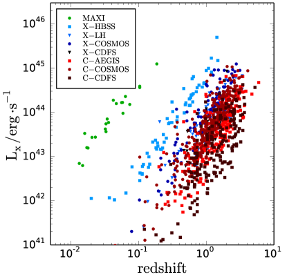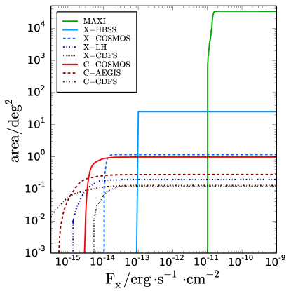(a)	(b)

Figure 1: (a) $\rm{5-10\,keV}$ luminosity - redshift plane, showing sources with either spectroscopic or photometric redshift estimation. (b) Sky coverage as a function of X-ray flux for each survey.

MAXI extragalactic survey

The Monitor of All-sky X-ray Image (MAXI) mission on board the International Space Station (ISS) observes the entire sky every 92 minutes with two instantaneous fields of view covering each $\rm{160^{\circ}\times 3^{\circ}}$. MAXI consists of two cameras, the Gas Slit Camera (GSC; Sugizaki et al. 2011; Mihara et al. 2011) sensitive in the $\rm{2-30\,keV}$ energy band and the Solid-state Slit Camera (SSC; Tsunemi et al. 2010; Tomida et al. 2011) sensitive in the $\rm{0.5-12\,keV}$ energy band. Hiroi et al. (2011) presented the first MAXI/GSC seven-month data catalog of sources detected in the $\rm{4-10\,keV}$ band and at high Galactic latitudes ($|b|>10^{\circ}$, $\rm{34,000deg^{2}}$). Ueda et al. (2011) used 37 AGN from this catalog to compute the local AGN luminosity function. Here we are using the 22 AGN out of the 37 AGN presented in Ueda et al. (2011) that have spectroscopic redshift $\rm{z>0.01}$. The flux limit of the sample is $\rm{F_{x}=1.1\times 10^{-11}erg\,s^{-1}\,cm^{-2}}$ covering a redshift range $0.01<z<0.19$ with median redshift $\rm{z=0.034}$ and median luminosity $\rm{\log L_{x}=43.85}$.

Hard Bright Serendipitous Survey (HBSS)

The XMM-Newton Bright Serendipitous Survey covers 25 $\rm{deg^{2}}$ (Della Ceca et al. 2004) and provides two flux limited samples in the $\rm{0.5-4.5\,keV}$ and $\rm{4.5-7.5\,keV}$ band. We are using the hard sample $\rm{4.5-7.5\,keV}$ with a flux limit of $\rm{F_{x}=1\times 10^{-13}erg\,s^{-1}\,cm^{-2}}$. The optical counterparts and spectroscopic redshifts are presented in Caccianiga et al. (2008). The sources cover the redshift range $0.02<z<1.48$ with median redshift $\rm{z=0.312}$ and median luminosity $\rm{\log L_{x}=43.8}$. This survey covers a large area introducing sample rare bright objects at higher redshift compared to MAXI.

XMM-COSMOS

The XMM-COSMOS field is one of the widest contiguous XMM fields covering 2 $\rm{deg^{2}}$. The XMM-COSMOS field contains 245 sources detected in the $\rm{5-10\,keV}$ (Cappelluti et al. 2009), with a flux limit of $\rm{F_{x}=5\times 10^{-15}erg\,s^{-1}\,cm^{-2}}$ and a good balance between depth and sky coverage. The unprecedented multiwavelength coverage of this field provides optical (Capak et al. 2007), ultraviolet (Zamojski et al. 2007), near-infrared (McCracken et al. 2010), mid-infrared (Sanders et al. 2007; Ilbert et al. 2009; Frayer et al. 2009) counterparts, and spectroscopic redshifts (Trump et al. 2009; Lilly et al. 2007, 2009) (see Brusa et al. 2007, 2010, for a summary). For 79.2% of the sample spectroscopic redshifts are available, while the remaining 18.3% of the sample has high quality photometric redshifts (Salvato et al. 2009, 2011) reaching a total of 97.5% redshift completeness. The X-COSMOS sources span a redshift range $0.04<z<3.14$, with a median redshift of $\rm{z=1.1}$ and median luminosity $\rm{\log L_{x}=44.05}$.

Table 1: Redshift information per X-ray field.

field	area	No. sources	spec-z	photo-z	no	median	completeness	redshift
	($\rm{deg^{2}}$)				redshift	redshift	completeness	range
MAXI	33800	22	22	0	0	0.04	100%	0.01-0.19
XMM-HBSS	25	64	62	0	2	0.31	96.9%	0.02-1.48
XMM-COSMOS	2.15/1.16	245/115	194/83	45/30	6/2	1.07/1.06	97.5%/98.3%	0.04-3.14
XMM-LH	0.2	88	50	38	0	1.19	100%	0.12-3.41
XMM-CDFS	0.26/0.12	137/30	109/18	24/8	4/4	1.31/1.22	97.1%/86.7%	0.12-3.8
Chandra-COSMOS	0.98	357	257	87	13	1.21	96.4%	0.04-4.1
Chandra-AEGIS-XD	0.28	244	133	111	0	1.51	100%	0.04-5.9
Chandra-CDFS	0.13	195	136	58	1	1.36	99.5%	0.1-5.2
total sample	33828	1115	761	332	22	1.19	98%	0.01-5.9

XMM - Lockman Hole (LH)

The Lockman Hole is one of the deepest XMM-Newton fields. The X-ray catalog presented in Brunner et al. (2008) contains 88 sources detected in the $\rm{5-10\,keV}$ band and the optical counterparts are presented in Rovilos et al. (2011) with flux limit $\rm{F_{x}=2\times 10^{-15}erg\,s^{-1}\,cm^{-2}}$. Photometric redshifts are presented in Fotopoulou et al. (2012) reaching 98.8% completeness. The Lockman Hole dataset provides faint sources detected with XMM, allowing us to probe the faint end of the luminosity function at redshift above 0.5. This dataset covers a redshift range of $0.118<z<3.41$ with median redshift $\rm{z=1.192}$ and median luminosity $\rm{\log L_{x}=43.78}$.

XMM - Chandra Deep Field South (XMM - CDFS)

The Chandra Deep Field South has been observed by XMM for a total exposure of 3.5 Ms. We include the $\rm{5-10\,keV}$ detections presented in Ranalli et al. (2013), where the optical identification and spectroscopic redshift sample is also described. The XMM observations reach a flux limit of $\rm{F_{x}=8\times 10^{-16}erg\,s^{-1}\,cm^{-2}}$. The photometric redshift described in Hsu et al. (2014) are specifically tuned for AGN and show improved accuracy over previous estimations for the same area. This dataset covers a redshift range of $0.5<z<2.5$ with median redshift $\rm{z=1.22}$ and median luminosity $\rm{\log L_{x}=43.58}$.

Chandra-COSMOS

The COSMOS field has also been observed with the Chandra observatory, and we use the $\rm{160\,ks}$ C-COSMOS observations of Elvis et al. (2009) covering an area of $\rm{{\sim}1.0\,deg^{2}}$. The reduction of the X-ray data is performed as described in Laird et al. (2009), yielding 357 sources detected in the $\rm{4-7\,keV}$ energy band with flux limit $\rm{F_{x}=1.8\times 10^{-15}erg\,s^{-1}\,cm^{-2}}$. The counterpart association and photo-z estimation are described in Aird et al. (2015). The Chandra-COSMOS sources span a redshift range $0.04<z<4.1$ with a median redshift of $\rm{z=1.2}$ and median luminosity $\rm{\log L_{x}=43.75}$.

AEGIS-XD

The AEGIS-XD field spans an area of $\rm{0.2\,deg^{2}}$ and benefits from multiwavelength coverage. The X-ray detection was performed with Chandra in the $\rm{4-7\,keV}$ energy range, and the counts were transformed to flux in the $\rm{5-10\,keV}$ range, assuming that the X-ray spectrum is a power-law with $\Gamma=1.4$ (Nandra et al. 2015). The optical counterparts were retrieved with a likelihood ratio approach, using the Rainbow Cosmological Surveys Database (Barro et al. 2011, a,b). Spectroscopic redshifts are a compilation from the DEEP2 (Newman et al. 2012) and DEEP3 fields (Cooper et al. 2012) and from the MMT (Coil et al. 2009). The AEGIS-XD survey is one of the two surveys with large number of objects in our sample with twice the area of LH and XMM-CDFS. The flux limit of AEGIS-XD is $\rm{F_{x}=5.9\times 10^{-16}erg\,s^{-1}\,cm^{-2}}$ and the sources cover the redshift range $0.05<z<3.85$ with median redshift $\rm{z=1.53}$ and median luminosity $\rm{\log L_{x}=43.64}$.

Chandra - Chandra Deep Field South (Chandra - CDFS)

The Chandra Deep Field South is the deepest to date X-ray field, covering an area of $\rm{0.1\,deg^{2}}$. We use the 4Ms observations (Xue et al. 2011), reduced as described in Laird et al. (2009), similar to the Chandra-COSMOS observations. The counterpart assignment is described in Aird et al. (2015), while the photo-z estimation are the same as for XMM-CDFS presented in Hsu et al. (2014). The flux limit of Chandra - CDFS is $\rm{F_{x}=1.4\times 10^{-16}erg\,s^{-1}\,cm^{-2}}$. The Chandra-CDFS contains 195 sources spanning a redshift range $0.1<z<5.2$ with a median redshift of $\rm{z=1.3}$ and median luminosity $\rm{\log L_{x}=43.2}$.

Avni & Bahcall (1980) introduced the coherent volume addition to analyze independent samples simultaneously. The main idea is that a source is considered detectable in any of the surveys as long as it is above the detection threshold for that particular survey. From the samples gathered for this work, sources in COSMOS and CDFS appear twice when considering both the XMM and Chandra observations since the fields partially overlap on the sky. Miyaji et al. (2015) solved this issue by merging the detection lists and creating an effective area curve that describes both XMM and Chandra COSMOS observations. Here instead we adopt a different strategy. Since both Chandra-COSMOS and Chandra-CDFS cover a smaller area than the respective XMM observations, we keep the entire Chandra field and select the XMM observations that do not fall in the Chandra area. With this approach, we have two independent fields profiting both from the depth of the Chandra observations and the wider area covered by XMM. In Table 1 we gather the area coverage, number of detected sources, and redshift information for all fields.

2.2 5-10 keV selection

AGN X-ray spectra above $\rm{1\,keV}$ can be described adequately as a power-law distribution, $F(E)\propto E^{-\Gamma}$, with $\Gamma{\rm=1.4-1.6}$ for radio loud AGN and $\Gamma\rm{=1.8-2.0}$ for radio-quiet AGN (Nandra & Pounds 1994; Reeves & Turner 2000; Piconcelli et al. 2005; Page et al. 2005; Mateos et al. 2005). We calculate theoretical flux and count rate values for different $\rm{N_{H}}$ and redshift values, assuming a power-law spectrum with photon index $\Gamma$ = 1.9 via models zphabs*cutoffpl in PyXspec, the Python interface to Xspec (Arnaud 1996). In Fig. 2 we plot the expected flux ratio for three $N_{H}$ values as a function of redshift. The blue lines correspond to the $\rm{5-10\,keV}$ energy band and the red lines correspond to the $\rm{2-10\,keV}$ energy band. We show that even for high absorbing column densities such as $\rm{10^{23}cm^{-2}}$, the observed flux in the $\rm{5-10\,keV}$ energy range is more than 90% of the intrinsic for $\rm{z>1}$, and never less than 80% even at lower redshifts. In this plot we do not include the effect of Thompson scattering, which would reduce the flux up to 2.3% and 18.8% in the $\rm{2-10\,keV}$ band at $\rm{\log N_{H}=22}$ and $\rm{\log N_{H}=23,}$ respectively.

Figure 2: Observed flux over intrinsic flux for a power-law spectrum with photoelectric absorption in the $\rm{5-10\,keV}$ band (blue) and $\rm{2-10\,keV}$ energy band (red). The observed $\rm{5-10\,keV}$ flux is never lower than 80% of the intrinsic at all redshifts column densities $\log N_{H}=23$.

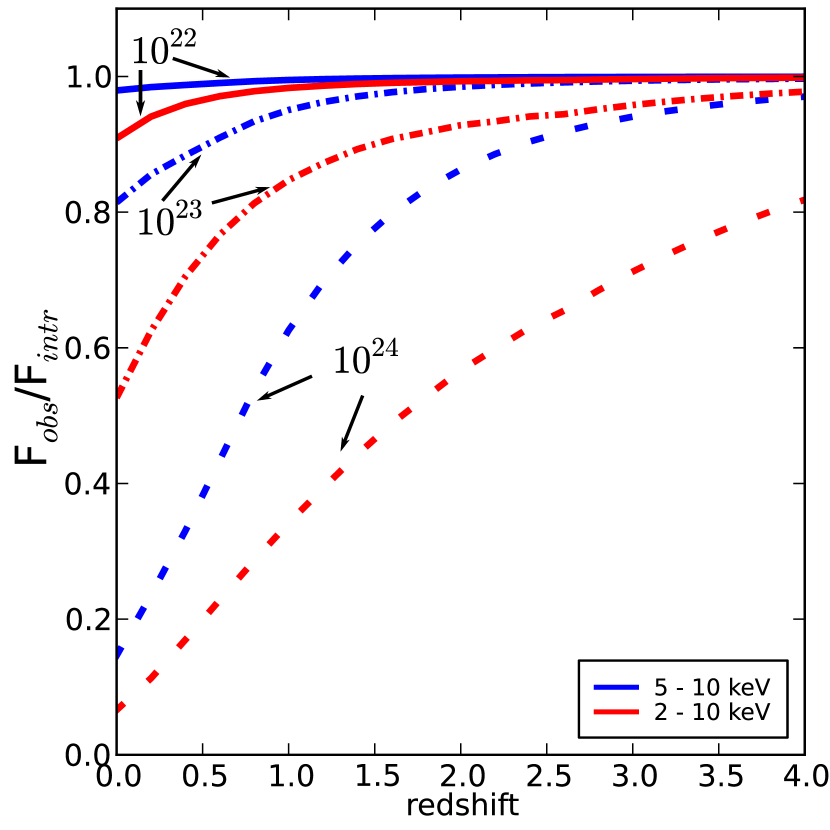
XMM-Newton and Chandra are less sensitive to energies above $\rm{7\,keV}$. Therefore, only bright sources are detected in the $\rm{5-10\,keV}$ energy band since typically the detection limit in this band is an order of magnitude higher compared to the $\rm{0.5-2\,keV}$ energy band. Consequently, this work does not include very faint sources ($\rm{F_{x}<5.9\times 10^{-16}erg\,s^{-1}\,cm^{-2}}$). Even though there are interesting cases on an individual source basis, we do not expect differences in a study of the global population as it has been demonstrated that the $\rm{5-10\,keV}$ does not select a special AGN population (Della Ceca et al. 2008).

3 Modeling the luminosity function

Early observations of X-ray AGN showed that the local luminosity function ($\rm{z{\sim}0}$) is well described by a broken power-law distribution (Maccacaro et al. 1983, 1984)

$$\frac{d\phi(L,z=0)}{d\log{L}}=\frac{A}{\left(\frac{L}{L_{0}}\right)^{\gamma_{1}}+\left(\frac{L}{L_{0}}\right)^{\gamma_{2}}},$$ (1)

where $L_{0}$, is the luminosity at which the break occurs and $\gamma_{1}$, $\gamma_{2}$ are the slopes of the power-law distributions below and above $L_{0}$.

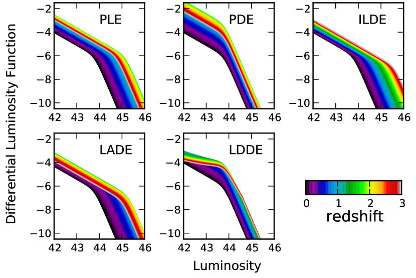
Several works thereafter have concluded that the luminosity function shows a strong evolution with redshift (e.g., Boyle et al. 1994; Page et al. 1996; Jones et al. 1997). We test the most commonly used models to describe the evolution of the luminosity function. In the rest of this section we give the formula and a brief physical description of each model. In Fig. 3 we show a qualitative overview of the differential luminosity function versus the luminosity computed at several redshifts given by the color scale. In these plots the critical redshift after which the evolution changes has been set to $z_{c}=1.8$ when applicable.

Figure 3: Comparison of common AGN luminosity function evolutionary models. Models computed with fictitious evolutionary parameters to demonstrate the qualitative difference in evolution. The color scale shows the evolution of each model with redshift ranging from z=0 (black) to z=3 (red). The critical redshift is chosen $z_{c}=1.8$ (bright green) for all models.

3.1 Pure luminosity evolution

The first modification of the broken power-law model to include evolution, PLE, was examined by Schmidt (1968). The evolution is most commonly expressed as (Miyaji et al. 2000; Ueda et al. 2003; La Franca et al. 2005; Ebrero et al. 2009)

$$\frac{d\phi(L,z)}{d\log L}=\frac{d\phi(L/e(z),z=0)}{d\log L}$$ (2)

with,

$$e(z)=\begin{cases}(1+z)^{p_{1}}&z\leq z_{c}\\ (1+z_{c})^{p_{1}}\cdot\left(\frac{1+z}{1+z_{c}}\right)^{p_{2}}&z\geq z_{c}\\ \end{cases},$$ (3)

where $z_{c}$ the redshift after which the evolution, $e(z)$, changes behavior and also follows a broken power law with slopes dependent on $p_{1}$ and $p_{2}$. As seen from Fig. 3, the PLE model is apparent as a shift of the luminosity function from higher to lower luminosities when moving from higher to lower redshift. Since the shape of the luminosity function is assumed to remain the same, this would be interpreted as a change in luminosity of the global AGN population.

3.2 Pure density evolution

The PDE model was also examined in the very early studies of luminosity function evolution (Schmidt 1968) and it is usually expressed as

$$\frac{d\phi(L,z)}{d\log L}=\frac{d\phi(L,z=0)}{d\log L}\cdot e(z),$$ (4)

with the evolutionary factor, $e(z),$ given by Eq. 3. The physical interpretation of this model is that AGN change in numbers, but their luminosities remain constant. This would be possible if the transition from active to inactive phase and vice versa were rapid and thus hardly observable. This evolution would appear as a change in the normalization of the luminosity function (see Fig. 3).

3.3 Independent luminosity density evolution

The ILDE model was used by Yencho et al. (2009) to describe the evolution of AGN for redshifts below z=1.2. This model postulates that there is a simultaneous change in luminosity and number of AGN. Since this model is confined below redshift z¡1.2, no critical redshift value was introduced, i.e.,

$$\frac{d\phi(L,z)}{d\log L}=\frac{d\phi(L/e_{L}(z),z=0)}{d\log L}e_{D}(z)$$ (5)

with,

$$e_{L}(z)=(1+z)^{p_{L}}$$ (6)

and

$$e_{d}(z)=(1+z)^{p_{D}},$$ (7)

similar to the PLE (Eq. 3) and PDE (Eq. 4) models below $z_{c}$.

3.4 Luminosity and density evolution

The LADE model was introduced by Aird et al. (2010). This model enables independent evolution of the luminosity function both in luminosity and number density, but with the inclusion of a critical redshift value,

$$\frac{d\phi(L,z)}{d\log L}=\frac{d\phi(L/e_{L}(z),z=0)}{d\log L}\cdot e_{d}(z).$$ (8)

The luminosity evolution follows a broken power law

$$e_{L}(z)=\left(\frac{1+z_{c}}{1+z}\right)^{p_{1}}+\left(\frac{1+z_{c}}{1+z}\right)^{p_{2}},$$ (9)

while the evolution in number density follows a power law given by

$$e_{d}(z)=10^{d(1+z)}.$$ (10)

3.5 Luminosity-dependent density evolution

The LDDE model was introduced by Schmidt & Green (1983) to describe the evolution of optically selected quasars. Miyaji et al. (2000) introduced a formalism to describe the soft X-ray luminosity function of type 1 (unabsorbed) AGN, which has been extensively used ever since. This more complex model encapsulates the fact that the number density of AGN changes, but since the evolution of bright and low-luminosity AGN exhibits different timescales, the critical redshift, $z_{c}$, depends on the luminosity.

We use the formalism introduced by Ueda et al. (2003) as follows:

$$\frac{d\phi(L,z)}{d\log L}=\frac{d\phi(L,z=0)}{d\log L}\cdot e(L,z)$$ (11)

with,

$$e(L,z)=\begin{cases}(1+z)^{p_{1}}&z\leq z_{c}(L)\\ (1+z_{c})^{p_{1}}\cdot\left(\frac{1+z}{1+z_{c}}\right)^{p_{2}}&z\geq z_{c}(L)\\ \end{cases}$$ (12)

and

$$z_{c}(L)=\begin{cases}z_{c}^{*}&L\geq L_{a}\\ z_{c}^{*}\cdot\left(\frac{L}{L_{a}}\right)^{a}&L<L_{a}\\ \end{cases}.$$ (13)

We express the evolution factor $e(L,z)$ of Eq. 12 as

$$e(z,L)=\frac{(1+z_{c})^{p_{1}}+(1+z_{c})^{p_{2}}}{\left(\frac{1+z}{1+z_{c}}\right)^{-p_{1}}+\left(\frac{1+z}{1+z_{c}}\right)^{-p_{2}}},$$ (14)

with $z_{c}$ defined as in Eq. 13. This formula is equivalent to the Ueda et al. (2003) evolution factor, creating a smooth transition of the XLF before and after the critical redshift, and it is normalized correctly at redshift zero.

Ueda et al. (2014), motivated by the results obtained by the COSMOS team at high redshift, (XMM-COSMOS; Brusa et al. (2009); Chandra-COSMOS; Civano et al. (2011)) introduced a more complicated model to describe the drop in number density above $\rm{z{\sim}3}$. In their formalism, an additional cutoff redshift is used, while the evolution index $\rm{p_{1}}$ is luminosity dependent as introduced by Miyaji et al. (2000). In Ueda et al. (2014), the evolutionary factor $\rm{e(L,z)}$ is given by

$$e(L,z)=\begin{cases}(1+z)^{p_{1}}&z\leq z_{c1}(L)\\ (1+z_{c1})^{p_{1}}\cdot\left(\frac{1+z}{1+z_{c1}}\right)^{p_{2}}&z_{c1}(L)<z\leq z_{c2}(L)\\ (1+z_{c1})^{p_{1}}\cdot\left(\frac{1+z_{c2}}{1+z_{c1}}\right)^{p_{2}}\cdot\left(\frac{1+z}{1+z_{c2}}\right)^{p_{3}}&z\geq z_{c2}(L)\\ \end{cases},$$ (15)

where

$$z_{c1,2}(L)=\begin{cases}z_{c1,2}^{*}&L\geq L_{a1,2}\\ z_{c1,2}^{*}\cdot\left(\frac{L}{L_{a1,2}}\right)^{a}_{1,2}&L<L_{a1,2}\\ \end{cases}$$ (16)

and

$$p_{1}(L)=p_{1}^{*}+\beta_{1}(\log{L}-\log{L_{p}}).$$ (17)

We refer to this expression of LDDE hereafter as Ueda14.

4 The $\rm{5-10\,keV}$ luminosity function

In this section, we present our procedure for the parameter estimation for the aforementioned models. We identify the model that best describes our dataset based on the Akaike information criterion (AIC) and Bayesian information criterion (BIC).

4.1 Model parameter estimation

According to the Bayes theorem, the posterior probability of the model parameters $\theta$, given the observed data $D$ and the model $M$, $p(\theta|D,M)$, is proportional to the probability of prior knowledge of the model parameters $\theta$, $p(\theta|M)$, times the likelihood of observing the collected data $D$, under the given model $M$ and set of model parameters $\theta$, $p(D|\theta,M)$as follows:

$$p(\theta|D,M)=\frac{p(\theta|M)p(D|\theta,M)}{\int p(\theta|M)p(D|\theta,M)d\theta}.$$ (18)

Treating the observation of $n$ sources out of the available $N$ AGN in the Universe as a Poisson process (applicable in the limit $n/N\ll 1$) (Marshall et al. 1983), the likelihood of observing $n$ sources is given by

$$\begin{split}\ln\mathcal{L}(L,z)=&\sum_{i=1}^{n}\ln\int\int{\phi(z_{i},\log L_{xi})}p_{i}(\log{L},z)\frac{dV_{c}}{dz}dzd\log{L}\\ &-\int\int\phi(z,\log L)\Omega(z,\log L)\frac{dV_{c}}{dz}dzd\log L\end{split},$$ (19)

where $\phi(z,\log L)$ is the model of the luminosity function, $\rm{p(\log{L},z)}$ the uncertainties on the luminosity and redshift for each observed source, $dV_{c}/dz$ the differential comoving volume, and $\Omega(z,\log L)$ the area curve of the survey.

Since X-ray counts and background counts are not available for all sources in our sample, we treat X-ray fluxes as delta functions. Hence, the uncertainties in Eq. 19 reduce to the uncertainties on the redshift estimation. In a similar fashion to Aird et al. (2010), we introduce the full probability distribution function of the photometric redshift estimates in our computation. The photometric redshifts in our sample (XMM-COSMOS, LH, XMM-CDFS, and AEGIS-XD) were computed in a consistent way with special treatment for AGN, i.e., including hybrid templates and applying proper prior information on the absolute magnitude as defined in Salvato et al. (2011).

We use noninformative distributions of priors for all parameters. The expected range for each parameter is determined from previous works on the AGN luminosity function in the $\rm{2-10\,keV}$ band, however, we do not wish to assume any shape for the distribution of the parameters.

To perform Bayesian analysis, we used MultiNest (Feroz, F. & Hobson, M. P. 2008; Feroz et al. 2009, 2013) through its python wrapper PyMultiNest(Buchner et al. 2014). MultiNest performs Nested Sampling introduced by Skilling et al., (2004) and is able to explore the posterior even in the case of multimodal distributions.

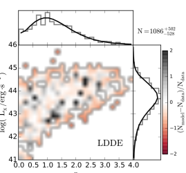
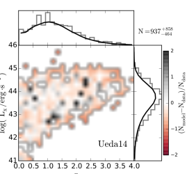
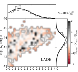
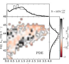
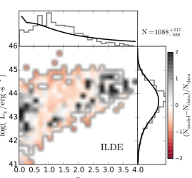
In Fig. 4 we plot the residuals between the model prediction and observed data for all models $(N_{model}-N_{data})/N_{data}$. All models are able to reproduce the total number of AGN observed (1105 objects available with redshift in our sample), albeit with about 40%-50% uncertainty at 90% level. For each model, we also show the distribution in redshift (top panels) and in luminosity (right-hand panels). The gray histogram is the distribution of the observed data, while the solid black line is the prediction of each model. The redshift histograms indicate that the models do not capture the redshift spikes observed around $\rm{z=0.6}$ and $\rm{z=1.0}$. At low redshifts ($z<0.3$) we see that only the models LDDE and Ueda14 correctly capture the local luminosity function. LDDE best reproduces the one-dimensional distributions in redshift and luminosity and, at the same time, the two-dimensional representation, while Ueda14 shows a suppression in the predicted number of sources. At low redshift, both LADE and PLE show an underestimated number of sources close to $\rm{\log L_{x}}=43$ and an overestimated number of sources at low ($\rm{\log L_{x}}=42$) and high ($\rm{\log L_{x}}=44$) luminosities. Lastly, models PDE and ILDE appear unable to capture the change in number of AGN showing large islands of under- and overestimation of the number of AGN both at low and high redshifts.

Figure 4: Fractional difference between predicted and observed number of AGN in a luminosity-redshift bin (color scale). The computation of the volume and luminosity function was performed on a 1000x1000 grid. The plots are rebinned on a 25x25 grid. Top and right-hand panels show the distribution in redshift and luminosity, respectively. The histograms represent the data, while the black lines are the model estimation.

4.2 Model selection

We apply the following two tests to identify the model that describes our dataset best.

Akaike Information Criterion (AIC)

The AIC selects the model with the least information loss, penalizing models with a higher number of free parameters (Akaike 1974). Therefore, it incorporates the Occam’s razor, which among two equally plausible explanations prefers the simpler explanation. The AIC is computed as

$${\rm{AIC}}=2k-2\ln{\mathcal{L}},$$ (20)

where $k$ is the number of parameters present in the model and $\mathcal{L}$ the maximum likelihood value. The preferred model is that with the lowest AIC value.

Bayesian Information Criterion (BIC)

The BIC selects models according to their likelihood value computed in a similar fashion to AIC, but with a higher penalty for complicated models (Schwarz 1978). It is expressed as

$${\rm{BIC}}=k\cdot\ln{n}-2\ln{\mathcal{L}},$$ (21)

where $k$ is the number of parameters of the model and $n$ is the number of observations. The preferred model is that with the lowest BIC value. Models with difference less than six must also be considered.

Table 2: Model selection criteria. According to AIC and BIC, LDDE is the preferred model.

	LDDE	Ueda14	PLE	LADE	PDE	ILDE
$k$	9	15	7	8	7	6
$\Delta$ AIC	0	13	41	37	150	269
$\Delta$ BIC	0	43	31	32	140	254

In Table 2 we give the comparison between LDDE and all other models. Both AIC and BIC identify the LDDE as the preferred model. For the dataset considered in this work, both selection criteria point to the direction that no other model can serve as an alternative. We see that according to the model selection criteria, ILDE is the worst representation; see §4.1 (Fig. 4). From the simpler models, PDE performs worst than PLE. Additionally, we see that LADE, which allows an independent evolution in luminosity and number density, is comparable PLE. Since BIC includes 15 model parameters, it imposes a strong penalty on the LDDE formalism of Ueda et al. (2014) .

Table 3: LDDE parameter summary. We recommend the use of posterior draws sampled with MultiNest; available upon request.

Parameter	Prior Interval					Posterior Mode
						Mean		Standard
								Deviation
$\log L_{0}$	41.	0	–	46.	0	43.	77	000.	11
$\gamma_{1}$	-2.	0	–	5.	0	0.	87	0.	06
$\gamma_{2}$	-2.	0	–	5.	0	2.	40	0.	11
$p_{1}$	0.	0	–	10.	0	5.	89	0.	31
$p_{2}$	-10.	0	–	3.	0	-2.	30	0.	50
$z_{c}$	0.	01	–	4.	0	2.	12	0.	16
$\log L_{a}$	41.	0	–	46.	0	44.	51	0.	11
$\alpha$	0.	0	–	1.	0	0.	24	0.	02
$\log A$	-10.	0	–	-2.	0	-5.	97	0.	17

Figure 5: Differential luminosity function versus luminosity for different redshift bins. The number of sources in each bin is given on the top right of each point. The solid black line is the mode of the luminosity function distribution, the gray shaded area encloses the 99% credible interval. The dashed black line shows the estimated luminosity function at $\rm{z=0}$ for comparison. The two red lines show the estimated luminosity function when the two posterior modes are used separately. The points are the binned estimations of the luminosity function, according to the $\rm{1/V_{max}}$ method, and they are in excellent agreement with our model.

4.3 Results

In Table 3 we summarize the parameter estimation of the LDDE model. We report the uniform prior interval and the posterior mean and standard deviation for each parameter. From Eq. 1 we can see that parameters $\gamma_{1}$ and $\gamma_{2}$ are symmetric, which means that the posterior distribution contains two modes. These two modes are easily distinguished with MultiNest and summary statistics are provided for each mode (see also §5.1).

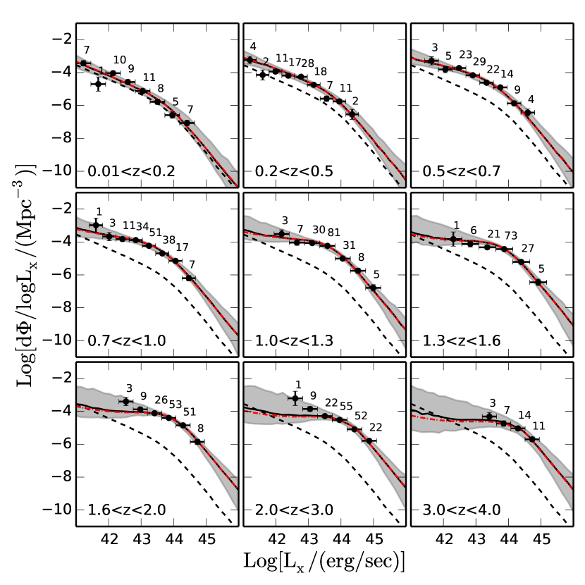
In Fig. 5 we plot the differential luminosity function for several redshift bins. The solid black line shows the peak of the distribution of the luminosity function at the median redshift of each redshift bin, while the gray shaded area encloses 90% probability of the differential luminosity function, $d\phi/dlogL_{x}$. To determine this area, we compute $d\phi/dlogL_{x}$ in each redshift bin for 40 values of the luminosity, $L_{x}$, for all the draws from the posterior. In this way, we naturally incorporate the true shape of the uncertainties for all parameters and their covariances. For reference, the dashed black line shows the luminosity function computed at redshift zero, using our model parameters in Eq. 1. The two (overlapping) red lines show the luminosity function when mode 1 and mode 2 are considered separately. As expected and demonstrated in Fig. 5, the estimation of the LF is better constrained in the (L-z) locus where observations are available and less constrained when extrapolating.

The black points are the result of the $1/V_{max}$ method. The $1/V_{max}$ method (Schmidt 1968) has been used widely in the literature to estimate the luminosity function of AGN. The advantage of this method is that the estimation is independent of any assumption on the underlying model. When a sizable sample of AGN is used, the computation of the luminosity function in thin redshift bins is powerful in revealing the presence of evolution. This computation also roughly reveals the shape of the XLF. Here we use the estimator proposed by Page & Carrera (2000)

$$\frac{d\phi(L,z)}{d\log{L}}=\frac{n}{\int_{\log{L_{min}}}^{\log{L_{max}}}\int_{z_{min}}^{z_{max}(L)}\Omega(z,\log L)\frac{dV}{dz}dz\,d\log{L}},$$ (22)

where $n$ is the number of AGN in the bin $[L_{min},L_{max}]$, and $[z_{min},z_{zmax}(L)]$. The value $z_{max}(L)$ corresponds to the maximum redshift up to which the $n$ sources would be still present in the sample, and this value is either the maximum redshift of the redshift bin or is given by the flux limit. Since it is a model independent method, it serves as a check for our fitting result.

5 Discussion

5.1 Information per survey

Figure 6: Marginal probability distribution function for LDDE parameters per survey. The gray shaded area shows the distribution of the parameters when all the fields are considered. The colored lines show the luminosity function parameters determined separately in each field. Flat distribution means that no information is present in a given survey about a particular model parameter.

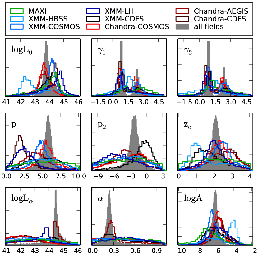
In Fig. 6 we show the marginal posterior distribution of each parameter for the LDDE model. The gray shaded area represents the XLF parameter distribution when we take all of the surveys we used into account. The colored lines represent the LDDE parameters estimated from each survey independently. In a maximum likelihood estimation, a method commonly used in previous works, one would be forced to fix one or more evolutionary parameters to gain some perspective on the local luminosity function when using a shallow survey such as MAXI. One of the advantages of our analysis is exploring the posterior without having to assume any specific shape for the likelihood. All parameters are left free and any dataset can be used to extract information, even for complicated models. For example, as seen in Fig. 6 MAXI (green) and HBSS (light blue) carry essentially no information about $L_{a}$, and $a$. Therefore, the marginal distribution for these parameters has the same shape as the prior, which in our case was a flat distribution. On the other hand, the deepest fields AEGIS-XD (red), and XMM-CDFS (black) are able to put constraints on the evolution parameters.

We can quantify the information gained and encoded in the posterior distribution compared to the prior information using the Kullback-Leibler divergence (Kullback and Leibler 1951)

$${\rm{D_{KL}((P||Q)}}=\int_{-\infty}^{+\infty}p(x)\log_{2}\frac{p(x)}{q(x)}dx,$$ (23)

where P and Q are two continuous random variables and p, q are their corresponding probability density functions. The information gain is measured in bits since the logarithm with base 2 is used. In Table 4 we show the information gain per survey and for combinations of surveys. In general, the shallow surveys provide higher information content on the LDDE parameters that describe the local XLF ($\rm{\log L_{0}}$, $\rm{\gamma_{1}}$, $\rm{\gamma_{2}}$) and the overall normalization ($\rm{A}$). On the other hand, deep surveys provide information on the evolution of the XLF with redshift ($\rm{p_{1}}$, $\rm{p_{2}}$). The luminosity dependence of the density evolution is constrained by the deepest fields, LH and AEGIS. The only field that does not conform to the expectation is Chandra-CDFS from which we find information gain for all model parameters, apart from parameter $\rm{\alpha}$.

Both astrophysical and systematic effects contribute to differences observed in the information present in each survey. Astrophysical effects include cosmic variance due to the presence of structures (e.g., clusters of galaxies), which would affect most the small-area fields (LH, XMM-CDFS, AEGIS). Also, because of the trade-off between depth and area covered by each survey, there is a lack of low-luminosity sources at higher redshifts. If a certain population (type I vs II, or highly obscured AGN) is dominant at specific redshifts, this would bias our result. The biases introduced by astrophysical effects are effectively conquered by the combination of independent surveys.

Ideally, all data should be extracted in a homogeneous manner, but for technical reasons this is not always possible. Therefore, differences due to systematic effects include: 1) deviations in the calibration of the X-ray satellites; for instance, Lumb et al. (2001) and Tsujimoto et al. (2011) reported a 10-20% difference in flux between XMM-Newton and Chandra; 2) difference in adopted survey detection limits determining the inclusion or not of a source in the catalog, which also affects the determination of the area curve of the survey; and 3) assumptions on the power-law index when converting counts to fluxes and fluxes to luminosities. We tested the latter for the AEGIS-XD survey, comparing the evidence between $\Gamma=1.4$ and $\Gamma=1.9$. We find no difference in the preferred model in the two cases. The bottom panel of Table 4 shows the information gain when the surveys are considered in a coherent way (Avni & Bahcall 1980). The combination of all XMM surveys provides enough information to constrain the behavior of the XLF at high redshifts through the model parameters $\rm{\log L_{\alpha}}$ and $\rm{\alpha}$. The Chandra surveys we consider cover a smaller area compared to the XMM surveys, but they are deeper that the XMM surveys. Runs 9 and 10 show the information gained when using only XMM surveys and only Chandra surveys, respectively. The parameter $\rm{p_{1}}$, which describes the evolution of the XLF below the critical redshift $\rm{z_{c}}$, is constrained better by the XMM surveys, while the high redshift evolution is constrained better by Chandra. In Table 5 we give the best-fit parameters for runs 9-14. There is notable difference between XMM-only and Chandra-only surveys. As seen from the information gain analysis, XMM surveys do constrain the high redshift evolution but with large uncertainties (20% on parameter $\alpha$). On the other hand, Chandra-only fields lead to a somewhat biased estimation of the XLF evolution at low redshift (parameter $\rm{p_{1}}\approx 7$). The reason for this discrepancy is the result of the area covered by the Chandra surveys, and not the result of systematic differences between the two instruments. At high redshift, both XMM and Chandra surveys converge to the same parameter estimation. The introduction of the MAXI survey significantly enhances the estimated XLF parameters, as seen by the information gained in Table 4.

Table 4: Prior-posterior information gain measured in bits on the marginal distribution of each model parameter. Zero bits means that the dataset carried no information regarding the specific parameter.

run	field selection			Information gain (bit)
				$\log L_{0}$		$\gamma_{1}$		$\gamma_{2}$		$p_{1}$		$p_{2}$		$z_{c}$		$\log L_{a}$		$\alpha$		$\log A$
1	MAXI			0.	67	0.	26	0.	40	0.	04	0.	03	0.	02	0.	05	0.	04	0.	53
2	XMM-HBSS			0.	54	0.	66	0.	38	0.	13	0.	10	0.	30	0.	13	0.	04	0.	76
3	XMM-COSMOS			1.	23	0.	97	0.	92	0.	77	0.	08	0.	59	0.	23	0.	04	1.	27
4	XMM-LH			0.	65	0.	58	0.	54	0.	66	0.	19	0.	52	0.	39	0.	09	0.	94
5	XMM-CDFS			0.	92	0.	74	0.	73	0.	24	0.	59	0.	31	0.	16	0.	18	0.	9
6	Chandra-COSMOS			1.	26	1.	2	1.	08	0.	73	0.	16	0.	63	0.	47	0.	05	1.	38
7	Chandra-AEGIS-XD			0.	88	0.	79	0.	93	0.	50	0.	31	0.	40	0.	41	0.	60	1.	28
8	Chandra-CDFS			0.	83	0.	72	0.	68	0.	91	0.	13	0.	28	0.	35	0.	05	1.	13
9	–	XMM	–	1.	54	1.	22	1.	40	1.	17	0.	53	0.	74	0.	35	0.	58	1.	63
10	–	–	Chandra	1.	51	1.	34	1.	24	0.	35	0.	89	0.	83	0.	63	0.	95	1.	91
11	–	XMM	Chandra	1.	81	1.	52	1.	57	1.	10	1.	02	0.	97	0.	87	1.	25	2.	09
12	MAXI	XMM	–	1.	65	1.	33	1.	29	1.	59	0.	58	0.	74	0.	38	0.	71	1.	67
13	MAXI	–	Chandra	1.	63	1.	39	1.	31	1.	31	1.	09	0.	74	0.	78	1.	27	1.	82
14	MAXI	XMM	Chandra	1.	88	1.	57	1.	52	1.	59	1.	15	1.	01	1.	04	1.	53	2.	02

Table 5: LDDE parameter summary for runs 9-14.

Parameter	XMM		Chandra		XMM+Chandra		MAXI+XMM		MAXI+Chandra		MAXI+XMM+Chandra
$\log L_{0}$	43.	97 $\pm$ 0.19	43.	62 $\pm$ 0.14	043.	72 $\pm$ 0.12	044.	04 $\pm$ 0.15	0043.	77 $\pm$ 0.13	000043.	77 $\pm$ 0.11
$\gamma_{1}$	0.	97 $\pm$ 0.07	0.	92 $\pm$ 0.09	0.	86 $\pm$ 0.06	0.	99 $\pm$ 0.07	0.	86 $\pm$ 0.06	0.	87 $\pm$ 0.06
$\gamma_{2}$	2.	53 $\pm$ 0.22	2.	46 $\pm$ 0.17	2.	37 $\pm$ 0.11	2.	65 $\pm$ 0.22	2.	43 $\pm$ 0.16	2.	40 $\pm$ 0.11
$p_{1}$	5.	72 $\pm$ 0.51	7.	02 $\pm$ 0.93	6.	03 $\pm$ 0.45	5.	72 $\pm$ 0.36	5.	92 $\pm$ 0.38	5.	89 $\pm$ 0.31
$p_{2}$	-2.	72 $\pm$ 1.14	-1.	81 $\pm$ 0.56	-2.	19 $\pm$ 0.54	-2.	72 $\pm$ 1.07	-2.	19 $\pm$ 0.56	-2.	30 $\pm$ 0.50
$z_{c}$	2.	19 $\pm$ 0.35	1.	99 $\pm$ 0.21	2.	08 $\pm$ 0.17	2.	28 $\pm$ 0.36	2.	15 $\pm$ 0.25	2.	12 $\pm$ 0.16
$\log L_{a}$	44.	55 $\pm$ 0.34	44.	48 $\pm$ 0.10	44.	49 $\pm$ 0.11	44.	68 $\pm$ 0.34	44.	53 $\pm$ 0.17	44.	51 $\pm$ 0.11
$\alpha$	0.	26 $\pm$ 0.05	0.	26 $\pm$ 0.03	0.	25 $\pm$ 0.02	0.	24 $\pm$ 0.04	0.	24 $\pm$ 0.02	0.	24 $\pm$ 0.02
$\log A$	-6.	26 $\pm$ 0.28	-6.	04 $\pm$ 0.24	-5.	92 $\pm$ 0.18	-6.	38 $\pm$ 0.24	-5.	98 $\pm$ 0.20	-5.	97 $\pm$ 0.17

5.2 Luminosity function evolution

Previous works in the $\rm{2-10\,keV}$ band have shown that the evolution of the AGN luminosity function is best described by the LDDE model (Ueda et al. 2003; La Franca et al. 2005; Silverman et al. 2008; Ebrero et al. 2009; Yencho et al. 2009; Ueda et al. 2014; Miyaji et al. 2015; Aird et al. 2015). The comparison among these works and the work presented here is not straightforward, as the sample selection and treatment vary. For example, each work treats corrections for intrinsic absorption and corrections for redshift incompleteness differently. Additionally, not all models are tested in the literature for compliance with each dataset, and the most commonly used are the PLE and LDDE models.

With this work we treat most of the analysis shortcomings found in earlier literature. We take photometric redshift uncertainties for all sources into account, assuming a flat redshift probability distribution between $z=0-7$ for sources with no redshift estimation. As discussed in §5.1, we do not fix any of the evolutionary parameters, since it is not needed within the Bayesian framework adopted for our analysis. Also, the $\rm{5-10\,keV}$ energy band chosen allows us to estimate the luminosity function of AGN, avoiding assumptions about the obscuration based on hardness ratios that could lead to a biased estimation of the absorbing column density (Brightman & Nandra 2012).

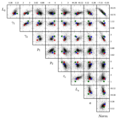
In Fig. 7 (a) we provide a visualization of the MultiNest draws for our best model (black points). There are significant correlations between the model parameters that must not be neglected during the model parameter estimation, for example, by fixing model parameters. We also plot on the same figure the best parameter point estimates of Ueda et al. (2014) (blue), Miyaji et al. (2015) (green), and Aird et al. (2015) (red). We see that all model estimations agree on the break luminosity $\rm{\log L_{0}}$, the normalization and high redshift $\rm{z_{c}}$ evolution given by $\rm{\log L_{\alpha}}$ and $\alpha$ parameters. On the other hand, there is disagreement on the slopes of the XLF and their evolution with redshift. The surveys we use for all of the analyses contain strong evidence to constrain the break points in the XLF model, namely $\rm{\log L_{0}}$, $\rm{z_{c}}$, $\rm{\log L_{\alpha}}$. The exact shape, however, depends upon the quality of the redshift measurement, spec-z vs photo-z, and if the full PDF is taken into account. Additionally, the presence of absorption is an extra modeling factor that can introduce bias in the estimation of the XLF. By selecting objects in the $\rm{5-10\,keV}$ energy band, we remove the effects of this extra set of model assumptions.

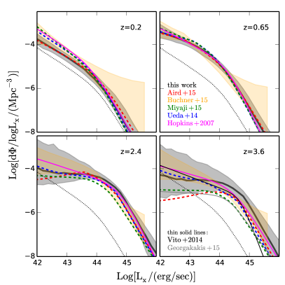
In Fig. 7 (b) we show our result transformed to the $\rm{2-10\,keV}$ energy band assuming AGN spectra can be described by a power law with $\Gamma=1.9$ (black solid line, dark gray area: 90% credible interval) and recent results from the literature (magenta, Hopkins et al. (2007); blue, Ueda et al. (2014); green, Miyaji et al. (2015); yellow, Buchner et al. (2015); red, Aird et al. (2015) ) for four redshift intervals. There is a remarkable agreement between all results up to redshift 2.5, and any small deviations are within the uncertainties.

Despite the many efforts of deep X-ray programs, the AGN XLF above z=3 is still under debate. Brusa et al. (2009) noted that the high redshift number density of AGN in the XMM-COSMOS field showed a decline that is more rapid than the predictions of the XLF models. The same trend was found in the Chandra-COSMOS observations by Civano et al. (2011). In the last panel of Fig. 7 (z=3.6) we plot two more literature results from Vito et al. (2014) (thin black line) and Georgakakis et al. (2015) (thin gray line). Both works provide a parametric model estimation of the AGN XLF at 3¡z¡5. We see that the estimates cluster in two regimes: a significant drop in the number density (Miyaji et al. 2015; Aird et al. 2015; Georgakakis et al. 2015) and a shallower drop in the number density (Hopkins et al. 2007; Ueda et al. 2014; Vito et al. 2014; Buchner et al. 2015). Our work is in agreement with the latter group and especially with the novel nonparametric XLF estimate of Buchner et al. (2015). Even though Ueda et al. (2014) proposed a more complicated formalism for the LDDE model to take the change of the AGN number density at $\rm{z>3}$ into account, our work shows that at least up to redshift four, there are a set of model parameters able to describe the AGN XLF without introducing extra complexity in the LDDE model.

(a)	(b)

Figure 7: (a) Posterior draws from MultiNest (black) and comparison with the point estimates from Ueda et al. (2014) (blue), Miyaji et al. (2015) (green), Aird et al. (2015) (red). Comparison of $\rm{5-10\,keV}$ luminosity function (black line) transformed to $\rm{2-10\,keV}$ to literature results. The gray area shows the 90% credible interval. Our result is in excellent agreement with the literature up to $z=2.5$. At high redshift our result shows a less prominent drop in the faint end of the XLF compared to estimations from Miyaji et al. (2015) (green), Aird et al. (2015) (red), and Georgakakis et al. (2015) (thin black line).

5.3 AGN number density

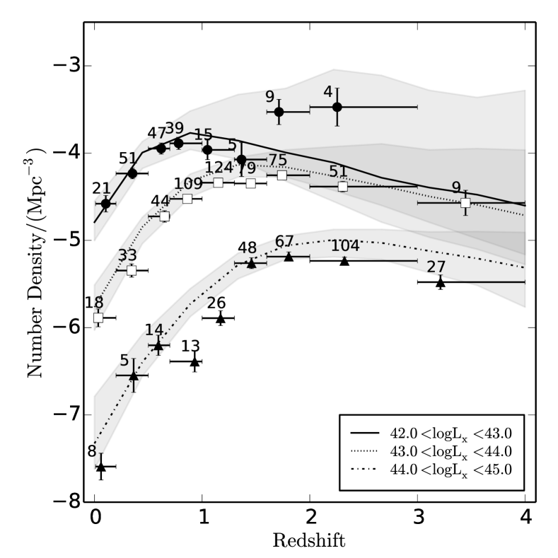
In Fig. 8 we plot the number density as a function of redshift for three luminosity bins. Our dataset shows the antihierarchical growth of black holes that has been observed previously in soft ($\rm{0.5-2\,keV}$) and hard ($\rm{2-10\,keV}$) energy bands. At the brightest luminosity range ($\rm{44<\log L_{x}<45}$), the number density for this dataset shows more of a flattening than a drop, in contrast to the estimations of Brusa et al. (2009), Civano et al. (2011), and Kalfountzou et al. (2014). Ueda et al. (2014) fix their second critical redshift at $\rm{z=3}$. Miyaji et al. (2015) use a sample of 3200 AGN in the $\rm{2-10\,keV}$ band and demonstrate that a second break is present between $\rm{z=2-3}$ after which a decline in the number density is observed. Our dataset is not numerous enough at $\rm{z>3}$ to support a more complicated evolution for AGN.

The antihierarchical growth of supermassive black holes, as imprinted on the AGN luminosity function, might seemingly be in stark contrast with the hierarchical structure formation within the framework of $\Lambda$CDM cosmology. Through hydrodynamic simulations and semi-analytic modeling, it has been shown that it is possible to qualitatively reconcile structure formation and AGN activity. Nevertheless, semi-analytic models are not able to rule out AGN evolutionary models or pinpoint the exact mechanism behind downsizing at this stage. Still largely debated in the literature, the predicted AGN luminosity function, from hydrodynamic simulation and semi-analytic modeling, is subject to the adopted AGN light curve and lifetime, obscuration, triggering mechanism, and feedback.

For example, in Fanidakis et al. (2011) the authors assumed that accretion takes place in two distinct modes, radiatively efficient and radiatively inefficient mode. Combining their semi-analytical model with the obscuration prescription from Hasinger (2008), they show that the bright end of the luminosity function is populated by quasars emitting close to the Eddington limit, while the faint end of the luminosity function is populated by black holes that undergo quiescent accretion. Hirschmann et al. (2014) showed that their hydrodynamic simulation is able to reproduce the observed downsizing at redshifts $z=0-5$, also allowing for cold gas accretion and major mergers. These authors mainly attribute the observed behavior to the gas density in the vicinity of the black hole, and they find the evolution of the gas reservoir was a consequence of star formation and AGN feedback. They also allow for obscuration in their models, following Hasinger (2008).

Even though dust obscuration can clearly enhance the observed flattening of the faint end of the luminosity function, which is particularly true for the soft X-ray band, the fact that downsizing is also observed in the $\rm{5-10\,keV}$ band, where the effect of the obscuration is minimal, points to the fact that this is not the predominant factor that shapes the AGN luminosity function. Hopkins et al. (2006) interpreted the AGN luminosity function in terms of quasar lifetimes and found good agreement between their simulations and the LDDE model, i.e., flattening of the faint end of the luminosity function. They claim that the observed break in the luminosity function corresponds to the maximum of the peak luminosity distributions of quasars at a certain redshift. The bright end of the luminosity function is populated by quasars that emit at their peak luminosity, while the faint end is populated by quasars that emit at lower luminosities. In their modeling, quasars spend the majority of their lifetime below their peak luminosity while, at the same time, more luminous objects transit to a less luminous stage faster than objects with lower peak luminosity. This implies that the slope of the faint end of the luminosity function is flatter at higher redshift. More recently, Enoki et al. (2014), assuming only major merger driven AGN triggering and no obscuration effects, showed that a combination of parameters could reproduce the observed downsizing: 1) cold gas depletion due to star formation; 2) scaling of the AGN lifetime with the dynamical time, in which high redshift AGN has a shorter dynamical time; and 3) suppression of gas cooling in massive dark matter halos.

Figure 8: Number density as a function of redshift for three luminosity bins showing the antihierarchical growth of black holes. The number of AGN per bin are given above each point.

5.4 Future surveys

With an anticipated detection of millions of AGN in the $\rm{0.5-2\,keV}$ energy range at a flux limit of $\rm{f_{0.5-2\,keV}=10^{-14}erg\,sec^{-1}cm^{-2}}$, eROSITA will mark a new era in the study of AGN. Over the $\rm{2-10\,keV}$ energy range, the brighter flux limit of $\rm{f_{2-10\,keV}=4\,10^{-14}erg\,sec^{-1}cm^{-2}}$ will allow the detection of hundreds of thousands of AGN (Merloni et al. 2012).

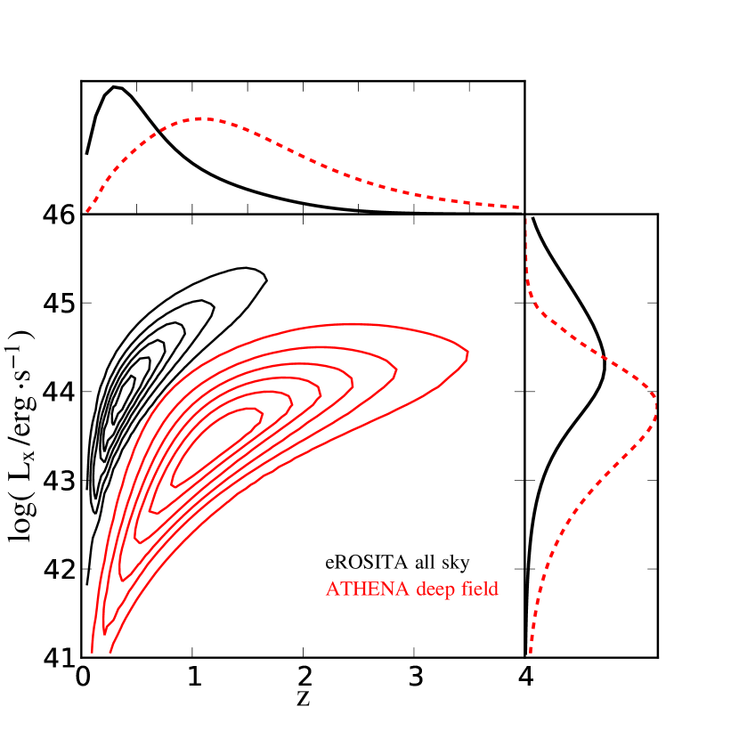
Transforming our $\rm{5-10\,keV}$ luminosity function in the $\rm{2-10\,keV}$ energy band and assuming an unabsorbed power law with photon index $\Gamma=1.9,$ we predict a total of $\rm{1.8\cdot 10^{5}}$ unabsorbed AGN in the range $\rm{0.01<z<4}$ and $\rm{41<\log L_{x}<46,}$ assuming 80% of the sky is accessible. This number is in good agreement with the prediction of Kolodzig et al. (2013), which anticipated 130 000 AGN in the four-year survey over $\rm{34100\,deg^{2}}$. In Figure 9 (black contours) we show the expected number of AGN detected with eROSITA. The coverage of the L_x-z plane will not be homogenous, and the majority of the detected sources are close to the break of the luminosity function at redshift 0.5. The eROSITA all-sky survey will measure the local luminosity function of AGN and its evolution up to $\rm{z=1}$. At higher redshifts, constraints on the bright end of the luminosity function will be possible. The top and right-hand histograms show the expected number distributions of AGN in redshift and luminosity, respectively.

To determine the behavior of the AGN number density during the golden era of quasars at a comparable quality level to the sample provided by eROSITA, wide and deep surveys are needed. The ATHENA mission will be able to provide such observations. The red contours in Fig. 9 show the expected number of AGN from ATHENA, assuming the multitiered survey strategy described in Aird et al. (2013) and Georgakakis et al. (2013), reaching a flux limit of $\rm{f_{2-10\,keV}=8\,10^{-17}erg\,sec^{-1}cm^{-2}}$ in the deepest area. The total anticipated number of AGN according to our model is $2.8\cdot 10^{5}$ AGN in the redshift range $\rm{0<z<4}$ and $\rm{8\,10^{4}}$ AGN in the redshift range $1<z<2$, which is below the break luminosity $\log L_{x}<44$. With the combination of these unprecedented samples of AGN, we will be able to provide the most accurate constraints on the luminosity function and its evolution.

Figure 9: Expected luminosity-redshift plane coverage from the all-sky survey with eROSITA (black curves) and ATHENA (red curves) in the $\rm{2-10\,keV}$ energy band. Top panel shows the predicted redshift distribution. Panel on the right shows the predicted luminosity distribution. The two missions complement each other and both are pivotal for a precise estimation of the AGN luminosity function.

6 Conclusions

Combining the most recent X-ray observations from MAXI, HBSS, XMM-COSMOS, XMM-LH, XMM-CDFS, Chandra-COSMOS, Chnadra-AEGIS-XD, and Chandra-CDFS in the $\rm{5-10\,keV}$ energy band, we compile a sample of 1100 AGN with 98% redshift completeness. We use the Chandra data in the inner region of the COSMOS and CDFS fields, and the XMM-Newton data in the outskirts where no Chandra data are available, to profit both from the depth and breadth of the observations. Our sample contains 68% spectroscopic redshifts and 30% very accurate photometric redshifts estimations from the fields XMM-COSMOS, XMM-LH, XMM-CDFS, Chandra-AEGIS-XD, Chandra-COSMOS, and Chandra-CDFS. Studying the $\rm{5-10\,keV}$ energy range, we avoid the potentially absorbed part of the spectrum for common $N_{H}$ values, effectively avoiding any assumption on otherwise necessary corrections to retrieve intrinsic X-ray luminosities.

Using Bayesian analysis we estimate the AGN $\rm{5-10\,keV}$ luminosity function and its evolution with redshift. Our results strongly support the luminosity-dependent density evolution (LDDE) model compared to PLE, PDE, LADE, and ILDE. We have demonstrated that by exploring the likelihood via MultiNest, we no longer need to fix model parameters even when there is not enough information in a dataset to constrain a complicated model. We quantify the information gain per XLF model parameter for the LDDE model for each individual field and for XMM and/or Chandra field combinations. We show that the evolution predicted by XMM-only and Chandra-only fields is varying, but this evolution remains consistent within the uncertainties at the 90% level.

We rule out the possibility of a pure density evolution. Our results demonstrate the presence of one critical redshift after which the evolution changes behavior and shows no evidence of a second critical redshift up to redshift four. Future work should focus on physically motivated evolutionary models, coupling the observed change in number density with AGN physics. We rule out the possibility of obscuration as the primary explanation for the observed antihierarchical growth of AGN.

Planned X-ray observatories will give an unprecedented view of the bright end of the luminosity function. We predict $1.8\cdot 10^{5}$ AGN up to $\rm{z=4}$ in the four-year, all-sky survey with eROSITA, while the multitiered survey strategy with ATHENA proposed in Aird et al. (2013) would provide the outstanding number of $10^{4}$ AGN at $1<z<2$ and $\log L_{x}<44$, which is sufficient to study the golden era of quasars and their coevolution with galaxies.