Depth and Reflection Total Variation for Single Image Dehazing

Abstract

Abstract- Haze removal has been a very challenging problem due to its ill-posedness, which is more ill-posed if the input data is only a single hazy image. In this paper, we present a new approach for removing haze from a single input image. The proposed method combines the model widely used to describe the formation of a haze image with the assumption in Retinex that an image is the product of the illumination and the reflection. We assume that the depth and reflection functions are spatially piecewise smooth in the model, where the total variation is used for the regularization. The proposed model is defined as a constrained optimization problem, which is solved by an alternating minimization scheme and the fast gradient projection algorithm. Some theoretic analyses are given for the proposed model and algorithm. Finally, numerical examples are presented to demonstrate that our method can restore vivid and contrastive hazy images effectively.

I Introduction

In foggy and hazy days, the light reflected from an object is usually absorbed and scattered by the turbid medium such as particles and water droplets in the atmosphere before it reaches the camera lens. Moreover, the light captured by the camera lens is often blended with the atmospheric light. This inevitably causes outdoor images taken in bad weather (e.g., foggy or hazy) to lose intensity contrast and color fidelity. Moreover, because most automatic systems strongly depend on the definition of the input images, they usually fail to work on the hazy images. Therefore, haze removal (or dehazing) is very important for the computer vision applications, such as remote sensing [13], video surveillance systems [27], and so on.

In computer vision and computer graphics, the model widely used to describe formation of a hazy image is that a hazy scene appearance is a weighted sum of the attenuated scene radiance and the transmitted atmospheric light whose extents depend on the scene distance to the camera lens (depth information) [29]. However, the depth information and the value of the atmospheric light are usually unknown in practice. Therefore, haze removal is a very challenging problem. The problem will be more ill-posed if the input data is only a single hazy image [8].

In the literature, there exist mainly two classes of approaches for removing haze. A class of approaches is dependent on multiple images or additional information. Polarization methods [20][21] remove haze by using the difference of the polarization characteristics from two or more images of the same scene taken with different polar angles. In [17][12][16], depth-based methods are proposed, which obtain the depth information from the user inputs or from known 3D models. These methods are effective for image dehazing, but they are somewhat impractical because both multiple images and a 3D geometrical model are usually difficult to acquire in practice.

Another class of approaches is to only use a single image to remove haze. This class can also be divided into two categories: filter methods and energy methods. The filter methods benefit from new image models or stronger priors. Fattal [4] recovered the haze-free scene contrast, under the assumption that the optical transmission and surface shading are not locally correlated to the estimation of the albedo of the scene and the optical transmission. Though Fattal’s assumption is physically reasonable, it is invalid when the haze is heavy or the assumption fails. Tan [22] removed haze by maximizing the local contrast of the restored image based on the observation that haze-free images have higher contrast than hazy images. Their results are greatly enhanced, but tend to be over-saturated, and the results may not be physically valid. Tarel and Hautière [23] introduced a fast algorithm to dehaze both color images and gray level images by using an edge preserving median filter. He et al. [8] proposed a dark channel prior (DCP) based on the observation that in most of the local regions it is very often that some pixels have very low intensity in at least one color (RGB) channel. Using this prior, they can recover high-quality haze-free images. However, this method has a high computational complexity in the soft matting process. After the DCP was proposed, the approaches based on this prior develop rapidly. In [9], He et al. proposed a guided image filtering in place of soft matting to speed up the process of dehazing. In [26], based on a physical model and the DCP, Wang et al. proposed a single image dehazing method which chooses the atmospheric light founded on a Variogram. Chen and Huang [2] presented a new image haze removal approach based on Fisher’s linear discriminant-based dual DCP scheme in order to solve the problems associated with the presence of localized light sources and color shifts, and thereby achieved effective restoration. In [3], Choi et al. proposed a referenceless perceptual fog density prediction model based on natural scene statistics (NSS) and fog aware statistical features. This model only makes use of measurable deviations from statistical regularities observed in natural foggy and fog-free images, which not only assesses the performance of defogging algorithms designed to enhance the visibility of foggy images, but also is well suited for image defogging. In [10], Huang et al. presented a novel Laplacian-based visibility restoration approach to solve inadequate haze thickness estimation and alleviate color cast problems. In [30], Dai et al. proposed an adaptive sky detection and preservation method to dehaze the images. The method detects the sky by hard or smooth threshold of the sky area which selects the threshold value as a function of the histogram of the image to process.

The energy methods usually propose an energy functional that should be minimized or maximized and derive a numerical scheme. Nishino et al. [19] proposed a Bayesian probabilistic dehazing method that jointly estimates the scene albedo and depth from a single foggy image by fully leveraging their latent statistical structures. Their method is effective for dehazing images but needs to tune a lot of parameters that have great influence on the final results. In [5], Fang et al. proposed a new energy model for dehazing and denoising simultaneously based on a windows adaptive DCP. In [6], Fattal derived a local formation model that explains the color-lines which means pixels of small image patches typically exhibit a 1D distribution in RGB color space and used it for recovering the scene transmission based on the lines’ offset from the origin. In [24], Wang et al. presented a multiscale depth fusion (MDF) method for defog from a single image. The fusion is formulated as an energy minimization problem that incorporates spatial Markov dependence. They got the depth map by minimizing the nonconvex potential in the random field which was solved by an alternate optimization algorithm. In [28], Zhu et al. proposed a Color Attenuation Prior to dehaze images. They recovered the depth information via creating a linear model for modeling the scene depth whose parameters are learned by a supervised learning method. In [7], Galdran et al. extended a perception-inspired variational framework for single image dehazing by substituting the mean of the clean image for the value of the gray-world hypothesis and adding a set of new terms to the energy functional for maximizing the interchannel contrast. In [14], Lai et al. derived the optimal transmission map directly from the haze model under two scene priors including locally consistent scene radiance and context-aware scene transmission. They introduced theoretic and heuristic bounds of scene transmission and incorporated the two scene priors to formulate a constrained minimization problem which solved by quadratic programming.

In this paper, we propose a new energy approach for removing haze from a single input image. Our model is a constrained total variation model which is deduced by combining the model widely used to describe the formation of a haze image with the assumption in Retinex that an image is the product of the illumination and the reflection. Then we use an alternating minimization scheme and the fast gradient projection (FGP) algorithm [1] to solve the proposed model and give some theoretical analysis for our model and the algorithm. At last, some experimental results are presented to show the effectiveness of our method.

The rest of our paper is organized as follows. In Section 2, we deduce the proposed model and show the existence and uniqueness of solution for the model. In Section 3, we present the algorithm to solve our model and investigate its convergence. In Section 4, we give the experimental results and conclude in Section 5.

II The proposed model

In computer vision and computer graphics, the formulation widely used to describe the hazy image is as follows [29]:

$$I(x)=t(x)J(x)+(1-t(x))A,\quad x\in\Omega,$$ (1)

where $I(x)$ is the observed intensity defined on the image domain $\Omega\subset{R^{2}}$ , $J(x)$ is the radiance of the surface, $A$ is a constant representing the globally atmospheric light, and $t(x)$ is the scene transmission describing the portion of the light that is not scattered and reaches the camera lens. When the atmosphere is homogenous, the transmission $t(x)$ can be formulated as [29]:

$$t(x)={e^{-\beta d(x)}},\quad x\in\Omega,$$ (2)

where $\beta$ is the positive scattering coefficient of the atmosphere and $d(x)$ is the depth of scene which is also positive.

According to the assumption widely used in Retinex [11][18][25][4][6], the surface radiance can be written as a product of the reflectance and the illumination:

$$J(x)=R(x)L(x),\quad x\in\Omega,$$ (3)

where $R(x)$ and $L(x)$ is the reflectance and the illumination, respectively. The reflectance $0\leq R(x)\leq 1$ is related to the physical characteristics of the surface. For the following theoretic analysis, we assume that $0\leq R(x)<1$ a.e. (almost everywhere). Based on the physical characteristics of the material object, the constraint $R(x)<1$ a.e. is practical.

Substituting (3) into (1), we have

$$I(x)=t(x)R(x)L(x)+(1-t(x))A,\quad x\in\Omega.$$ (4)

Because most hazy images are landscapes of outdoor scenarios, we make the following assumption:

$$L(x)\leq A,\quad x\in\Omega.$$ (5)

Since $R(x)<1$ a.e., by (4) and (5) we obtain

$$\begin{aligned} I(x)&=t(x)R(x)L(x)+A-t(x)A\\ &<t(x)A+A-t(x)A\\ &=A,\quad\text{a.e.}\;x\in\Omega.\end{aligned}$$ (6)

Equation (6) implies

$$A\geq ess{\sup_{x\in\Omega}}I(x).$$

Because the atmospheric light $A$ is a constant, we have

$$A=ess{\sup_{x\in\Omega}}I(x)+C_{0},$$

where $C_{0}\geq 0$ is a constant. By the way, by experiments we found that the proposed model is insensitive to the value of $C_{0}$ (or $A$), the assumption (5) is valid by choosing larger value of $C_{0}$.

Equation (4) can be rewritten as

$$1-\frac{{I(x)}}{A}=t(x)(1-\frac{{R(x)L(x)}}{A}),\quad x\in\Omega.$$ (7)

Let $R^{*}(x)=\frac{{R(x)L(x)}}{A}$. Because of (5), we have $0\leq R^{*}\leq R<1$. In particular, if $L(x)=A$, then $R^{*}=R$. In order to handle the product expression in (7), we convert the product to the logarithmic form. Let $i(x)=\log(1-\frac{{I(x)}}{A}),\quad\eta(x)=\log(t(x))=-\beta d(x),\quad\gamma(x)=\log(1-R^{*}(x)).$ Then, Equation (7) is equivalent to

$$i(x)=\eta(x)+\gamma(x),\quad x\in\Omega.$$

Besides, since $-\beta d(x)<0$ and $0<1-R^{*}(x)<1$, we have $\eta(x)\leq 0$, $\gamma(x)\leq 0$ and so $i(x)\leq\eta(x)$, $i(x)\leq\gamma(x)$. Therefore, the constraints $i\leq\eta\leq 0$ and $i\leq\gamma\leq 0$, a.e. need to be added into the proposed model.

It should be pointed out that Equation (7) has the similar form with Equation (8) in [19], but the deriving processes are different. We derive Equation (7) by merging the Retinex theory into the haze imaging model (1), while Nishino et al. [19] derive their model by rewriting the Koschmieder’s law. The constraint $\gamma(x)\leq 0$ is very important for our variational method (see Figure 10). However, this constraint cannot be obtained by Nishino et al.’ method of deriving Equation (8) in [19].

We further make the following assumptions before presenting our model:

• The depth function $\eta(x)$ and the reflection function $\gamma(x)$ are piecewise smooth in $\Omega$. Thus $\eta,\;\gamma\in BV(\Omega)$ and the regularization terms are defined by $\int_{\Omega}{\left|{\nabla\eta}\right|}$ and $\int_{\Omega}{\left|{\nabla\gamma}\right|}$.

• The sum of the depth function $\eta(x)$ and the reflection function $\gamma(x)$ is close to $i(x)$. Thus, the fidelity term is given by $\int_{\Omega}{{{(\eta+\gamma-i)}^{2}}}$.

Collecting the above two assumptions into one expression, we propose the following energy functional for dehazing:

$$E(\eta,\gamma)=\alpha\int_{\Omega}{\left|{\nabla\eta}\right|}+\int_{\Omega}{{{(\eta+\gamma-i)}^{2}}}+\beta\int_{\Omega}{\left|{\nabla\gamma}\right|}+\lambda\int_{\Omega}{\gamma^{2}},$$ (8)

where $\alpha>0$ and $\beta>0$ are regularization parameters and $\lambda>0$ is an arbitrary small constant.

The term $\lambda\int_{\Omega}{\gamma^{2}}$ is only used for the proof of the uniqueness of the minimizer. Without this term, a constant can be added to variable $\eta$ and subtracted to variable $\gamma$ without a change of the value of the energy functional. Numerically, there is no difference for our model with $\lambda$ being a very small value (such as $10^{-10}$) and $\lambda$ being zero. Therefore, we always set $\lambda=0$ in numerical implementation.

The proposed model is thus given by the constrained optimization problem:

$$\text{Minimize:}\quad\;E(\eta,\gamma),\;\;\;\eta,\;\gamma\in BV(\Omega)$$ (9)

$$\text{Subject to:}\quad i\leq\eta\leq 0\;,\;i\leq\gamma\leq 0,\;\text{a.e.}$$

We first show the existence of solution for the above optimization problem.

Theorem 1

The functional $E(\eta,\gamma)$ is strictly convex in $\left\{{(\eta,\;\gamma)|\;i\leq\eta,\gamma\leq 0}\right\}$.

The proof is trivial and so is omitted.

Theorem 2

If $i\in{L^{2}}(\Omega)$, then problem (9) has exactly one solution.

Proof:

First, the energy functional $E(\eta,\gamma)$ is clearly nonnegative and proper because $E(0,0)$ is a finite value. Let $({\eta_{n}},{\gamma_{n}})$ is a minimizing sequence of problem (9), i.e.,

$$\mathop{\lim}\limits_{n\to\infty}E({\eta_{n}},{\gamma_{n}})=\inf_{{\eta,\gamma\in BV(\Omega),i\leq\eta\leq 0,i\leq\gamma\leq 0}}E(\eta,\gamma).$$

Then, there is a constant $C>0$ so that

$$E({\eta_{n}},{\gamma_{n}})= \alpha\int_{\Omega}{\left|{\nabla{\eta_{n}}}\right|}+\int_{\Omega}{{{({\eta_{n}}+{\gamma_{n}}-i)}^{2}}}+\beta\int_{\Omega}{\left|{\nabla{\gamma_{n}}}\right|}$$

$$+\lambda\int_{\Omega}{\gamma_{n}^{2}}\leq C.$$

Thus,

$$\int_{\Omega}{\left|{\nabla{\eta_{n}}}\right|}\leq C/\alpha,\;\;\int_{\Omega}{\left|{\nabla{\gamma_{n}}}\right|}\leq C/\beta.$$ (10)

Since $i\in{L^{2}}(\Omega)$, $i\leq{\eta_{n}}\leq 0$ and $i\leq{\gamma_{n}}\leq 0$, we have

$$\int_{\Omega}{\eta_{n}^{2}}\leq\int_{\Omega}{{i^{2}}},\int_{\Omega}{\gamma_{n}^{2}}\leq\int_{\Omega}{{i^{2}}}.$$

By the Jensen’s inequality, we obtain

$$\int_{\Omega}{\left|{{\eta_{n}}}\right|}\leq{\left|\Omega\right|^{1/2}}{\left\|{{\eta_{n}}}\right\|_{{L^{2}}(\Omega)}}\leq{\left|\Omega\right|^{1/2}}{\left\|i\right\|_{{L^{2}}(\Omega)}},$$ (11)

$$\int_{\Omega}{\left|{{\gamma_{n}}}\right|}\leq{\left|\Omega\right|^{1/2}}{\left\|i\right\|_{{L^{2}}(\Omega)}}.$$

Namely, the sequences $\{{\eta_{n}}\}$ and $\{{\gamma_{n}}\}$ are bounded in ${L^{1}}(\Omega)$. Combining it with (10), we know that the sequences $\{{\eta_{n}}\}$ and $\{{\gamma_{n}}\}$ are bounded in $BV(\Omega)$. Hence, there exists some $({\eta_{*}},{\gamma_{*}})\in BV(\Omega)\times BV(\Omega)$ such that, up to a subsequence,

$${\eta_{n}}\to{\eta_{*}}\;\;\text{and}\;\;{\gamma_{n}}\to{\gamma_{*}}\;\;\text{in}\;{L^{1}}(\Omega),$$ (12)

$${\eta_{n}}\to{\eta_{*}}\;\;\text{and}\;\;{\gamma_{n}}\to{\gamma_{*}}\;\;\text{weakly in}\;{L^{2}}(\Omega).$$ (13)

By the (weak) lower semicontinuity of the ${L^{2}}-\text{norm}$ and (13), we have

$$\int_{\Omega}{{{({\eta_{*}}+{\gamma_{*}}-i)}^{2}}}\leq\mathop{\liminf}\limits_{n\to\infty}\int_{\Omega}{{{({\eta_{n}}+{\gamma_{n}}-i)}^{2}}}.$$ (14)

By (12) and the lower semicontinuity of $BV(\Omega)$, we have

$$\int_{\Omega}{\left|{\nabla{\eta_{*}}}\right|}\leq\mathop{\liminf}\limits_{n\to\infty}\int_{\Omega}{\left|{\nabla{\eta_{n}}}\right|}$$ (15)

$$\int_{\Omega}{\left|{\nabla{\gamma_{*}}}\right|}\leq\mathop{\liminf}\limits_{n\to\infty}\int_{\Omega}{\left|{\nabla{\gamma_{n}}}\right|}.$$

Recalling the semicontinuity of $L^{2}$ norm, by (13) we have

$$\int_{\Omega}{\gamma_{*}^{2}}\leq\mathop{\liminf}\limits_{n\to\infty}\int_{\Omega}{\gamma_{n}^{2}}.$$ (16)

Combining (14) and (15), we further have

$$E({\eta_{*}},{\gamma_{*}})$$

$$= \alpha\int_{\Omega}{\left|{\nabla{\eta_{*}}}\right|}+\int_{\Omega}{{{({\eta_{*}}+{\gamma_{*}}-i)}^{2}}}+\beta\int_{\Omega}{\left|{\nabla{\gamma_{*}}}\right|}+\lambda\int_{\Omega}{\gamma_{*}^{2}}$$

$$\leq \mathop{\alpha\liminf}\limits_{n\to\infty}\int_{\Omega}{\left|{\nabla{\eta_{n}}}\right|}+\mathop{\liminf}\limits_{n\to\infty}\int_{\Omega}{{{({\eta_{n}}+{\gamma_{n}}-i)}^{2}}}$$

$$+\mathop{\beta\liminf}\limits_{n\to\infty}\int_{\Omega}{\left|{\nabla{\gamma_{n}}}\right|}+\lambda\mathop{\liminf}\limits_{n\to\infty}\int_{\Omega}{\gamma_{n}^{2}}$$

$$\leq \mathop{\liminf}\limits_{n\to\infty}(\alpha\int_{\Omega}{\left|{\nabla{\eta_{n}}}\right|}+\int_{\Omega}{{{({\eta_{n}}+{\gamma_{n}}-i)}^{2}}}+\beta\int_{\Omega}{\left|{\nabla{\gamma_{n}}}\right|}+\lambda\int_{\Omega}{\gamma_{n}^{2}})$$

$$= \mathop{\liminf}\limits_{n\to\infty}E({\eta_{n}},{\gamma_{n}})$$

$$= \mathop{\lim}\limits_{n\to\infty}E({\eta_{n}},{\gamma_{n}})$$

$$= \mathop{\inf}\limits_{\eta,\gamma\in BV(\Omega),i\leq\eta\leq 0,i\leq\gamma\leq 0}E(\eta,\gamma).$$

Meanwhile, by (12) we have, up to a subsequence,

$${\eta_{n}}\to{\eta_{*}}\quad\text{and}\quad{\gamma_{n}}\to{\gamma_{*}}\quad\text{a.e. in}\;\Omega.$$ (17)

By $i\leq{\eta_{n}}\leq 0$ and $i\leq{\gamma_{n}}\leq 0$ a.e., we obtain that $({\eta_{*}},{\gamma_{*}})$ satisfies the constraints $i\leq{\eta_{*}}\leq 0$ and $i\leq{\gamma_{*}}\leq 0$, a.e.. Thus $({\eta_{*}},{\gamma_{*}})$ is a solution of problem (9). The uniqueness of the solution is guaranteed by the strictly convex of the functional $E(\eta,\gamma)$. ∎

III The algorithm

Since there are two unknown variables in problem (9), we use the alternating minimization scheme to convert it into two subproblems. We describe it in Algorithm 1 in detail.

Algorithm 1.

• Set initial value ${\eta_{0}}=i$, ${\gamma_{0}}=0$, $k=0$, predefined iterations ${N_{1}}>0$ and error tolerance $\varepsilon>0$.

• At the $k$th iteration:
  

  1. Given ${\gamma_{k}}$, compute ${\eta_{k+1}}$ by solving
     

     $$\mathop{\min}\limits_{i\leq\eta\leq 0}{E_{1}}(\eta)=\alpha\int_{\Omega}{\left|{\nabla\eta}\right|}+\int_{\Omega}{{{(\eta+{\gamma_{k}}-i)}^{2}}}.$$ (18)

  2. Given ${\eta_{k+1}}$, compute ${\gamma_{k+1}}$ by solving
     

     $$\mathop{\min}\limits_{i\leq\gamma\leq 0}{E_{2}}(r)=$$ (19)

     $$\beta\int_{\Omega}{\left|{\nabla\gamma}\right|}+\int_{\Omega}{{{(\gamma+{\eta_{k+1}}-i)}^{2}}}+\lambda\int_{\Omega}{\gamma^{2}}.$$

• Go back to step 2 until $\frac{{\left\|{{\eta_{k+1}}-{\eta_{k}}}\right\|}}{{\left\|{{\eta_{k+1}}}\right\|}}\leq\varepsilon\;\&\;\frac{{\left\|{{\gamma_{k+1}}-{\gamma_{k}}}\right\|}}{{\left\|{{\gamma_{k+1}}}\right\|}}\leq\varepsilon$ or $k={N_{1}}$.

Problems (18) and (19) are the constrained total variation minimal problems, which can be solved by the FGP algorithm [1] efficiently.

Suppose that the hazy image $I(x)$ is an $m\times n$ matrix. Let $p\in{R^{(m-1)\times n}}$, $q\in{R^{m\times(n-1)}}$ and $r\in{R^{m\times n}}$, define:

• The unit ball in ${R^{(m-1)\times n}}\times{R^{m\times(n-1)}}$:

  $$E=\left\{{(p,q)\left|{\begin{array}[]{*{20}{c}}{p_{i,j}^{2}+q_{i,j}^{2}\leq 1,\;\;{\begin{array}[]{*{20}{c}}{i=1,...,m-1,}\\ {j=1,...,n-1}\end{array}}}\\ {\left|{{p_{i,n}}}\right|\leq 1,\;\;\;\;\;\;\;\;\;\;\;i=1,...,m-1}\\ {\left|{{q_{n,j}}}\right|\leq 1,\;\;\;\;\;\;\;\;\;\;\;j=1,...,n-1}\end{array}}\right.}\right\}$$

• The divergence of $\left({p,q}\right)$:

  $${\left({{\mathop{\rm div}\nolimits}\left({p,q}\right)}\right)_{i,j}}=$$

  $$\left\{\begin{array}[]{l}{p_{i,j}}+{q_{i,j}}-{p_{i,j}}-{q_{i,j}},\;{\begin{array}[]{*{20}{c}}{i=1,...,m-1,}\\ {j=1,...,n-1}\end{array}}\\ 0,\;\;\;\;\;\;\;\;\;\;\;\;\;\;\;\;\;\;\;\;\;\;\;\;\;\;\;i=1,m,j=1,...,n\\ 0,\;\;\;\;\;\;\;\;\;\;\;\;\;\;\;\;\;\;\;\;\;\;\;\;\;\;\;i=1,...,m,j=1,n\end{array}\right.$$

• The gradient of $r$:

  $$\nabla(r)=(p,q),$$

  where

  $$p={r_{i,j}}-{r_{i+1,j}},\;\;i=1,...,m-1,j=1,...,n$$

  $$q={r_{i,j}}-{r_{i,j+1}},\;\;i=1,...,m,j=1,...,n-1$$

• The projection from $r$ on $C=[i,\;0]$:

  $${P_{C}}(r)=\min(\max(i,r),0)$$

• The projection from $(p,q)$ on $E$:

  $${\left({{P_{E}}(p,q)}\right)_{(i,j)}}=\left({\frac{{{p_{i,j}}}}{{\max(1,\left|{{p_{i,j}}}\right|)}},\frac{{{q_{i,j}}}}{{\max(1,\left|{{q_{i,j}}}\right|)}}}\right)$$

Then, according to Proposition 4.1 in [1], the solution ${\eta_{k+1}}$ of problem (18) can be written as

$${\eta_{k+1}}={P_{C}}\left[{i-{\gamma_{k}}-\alpha{\mathop{\rm div}\nolimits}(p,q)}\right],$$

where $(p,q)$ is the solution of the following problem:

$$\mathop{\min}\limits_{(p,q)\in E}h(p,q)= -{{\left\|{{H_{C}}(i-{\gamma_{k}}-\alpha{\mathop{\rm div}\nolimits}(p,q))}\right\|}^{2}}$$ (20)

$$+{{\left\|{i-{\gamma_{k}}-\alpha{\mathop{\rm div}\nolimits}(p,q)}\right\|}^{2}}$$

with ${H_{C}}(r)=r-{P_{C}}(r)$. Problem (20) is computed by

$$({p_{k}},{q_{k}})={P_{E}}({({l_{k}},{s_{k}})+\frac{1}{{8\alpha}}\nabla({P_{C}}\left[{i-{\gamma_{k}}-\alpha{\mathop{\rm div}\nolimits}({l_{k}},{s_{k}})}\right])}),$$ (21)

where $({l_{k}},{s_{k}})$ is obtained by an accelerated scheme from $({p_{k-1}},{q_{k-1}})$:

$${t_{k+1}}=\frac{{1+\sqrt{1+4t_{k}^{2}}}}{2},$$ (22)

$$({l_{k+1}},{s_{k+1}})=({p_{k}},{q_{k}})+\frac{{{t_{k}}-1}}{{{t_{k+1}}}}({p_{k}}-{p_{k-1}},{q_{k}}-{q_{k-1}}).$$

Thus, the FGP algorithm for Problem (18) is as follows:

Algorithm 2.

• Set initial values $({l_{1}},{s_{1}})=({p_{0}},{q_{0}})=0$, ${t_{1}}=1,$ $j=1$ and predefined iterations ${N_{2}}>0$.

• At the jth iteration:
  Given $({p_{j-1}},{q_{j-1}})$ and $({l_{j}},{s_{j}})$, Compute

  1. $({p_{j}},{q_{j}})$ by (21),

  2. ${t_{j+1}}$ and $({l_{j+1}},{s_{j+1}})$ by (22).

• $j=j+1$, go back to step 2 until convergence or $j={N_{2}}$.

• Set $output={P_{C}}\left[{i-{\gamma_{j}}-\alpha{\mathop{\rm div}\nolimits}({p_{j}},{q_{j}})}\right]$.

Since we set $\lambda=0$, we can solve problem (19) by the similar method.

Next, we investigate the convergence of Algorithm 1.

Theorem 3

Let $i\in{L^{2}}(\Omega)$ and $({\eta_{k}},{\gamma_{k}})$ be the sequence derived from Algorithm 1. Then the sequence $({\eta_{k}},{\gamma_{k}})$ converges to some $({\eta_{\#}},{\gamma_{\#}})\in BV(\Omega)\times BV(\Omega)$ (up to a sequence), and for any

$$(\eta,\gamma)\in\left\{{(\eta,\gamma)|\eta,\gamma\in BV(\Omega),i\leq\eta\leq 0,i\leq\gamma\leq 0,a.e.}\right\},$$

we have

$$E({\eta_{\#}},{\gamma_{\#}})\leq E({\eta_{\#}},\gamma),\quad E({\eta_{\#}},{\gamma_{\#}})\leq E(\eta,{\gamma_{\#}}).$$

Proof:

By (18) and (19), we have the following inequalities

$$E({\eta_{k+1}},{\gamma_{k+1}})\leq E({\eta_{k+1}},{\gamma_{k}})\leq E({\eta_{k}},{\gamma_{k}})\leq...\leq E({\eta_{0}},{\gamma_{0}}).$$

Thus, $E({\eta_{k}},{\gamma_{k}})$ is bounded and decreases with $k$. Because of

$$E({\eta_{k}},{\gamma_{k}})= \alpha\int_{\Omega}{\left|{\nabla{\eta_{k}}}\right|}+\int_{\Omega}{{{({\eta_{k}}+{\gamma_{k}}-i)}^{2}}}$$ (23)

$$+\beta\int_{\Omega}{\left|{\nabla{\gamma_{k}}}\right|}+\lambda\int_{\Omega}{\gamma_{k}^{2}}.$$

$$\leq E({\eta_{0}},{\gamma_{0}}),$$

we have

$$\int_{\Omega}{\left|{\nabla{\eta_{k}}}\right|}\leq E({\eta_{0}},{\gamma_{0}})/\alpha,\quad\int_{\Omega}{\left|{\nabla{\gamma_{k}}}\right|}\leq E({\eta_{0}},{\gamma_{0}})/\beta.$$ (24)

Since $i\in{L^{2}}(\Omega)$, $i\leq{\eta_{k}}\leq 0$ and $i\leq{\gamma_{k}}\leq 0$, we have

$$\int_{\Omega}{\eta_{k}^{2}}\leq\int_{\Omega}{{i^{2}}},\quad\int_{\Omega}{\gamma_{k}^{2}}\leq\int_{\Omega}{{i^{2}}},$$

which implies that $\{{\eta_{k}}\}$ and $\{{\gamma_{k}}\}$ are bounded in ${L^{2}}(\Omega)$ and so bounded in ${L^{1}}(\Omega)$. By (24), we obtain that $\{{\eta_{k}}\}$ and $\{{\gamma_{k}}\}$ are bounded in $BV(\Omega)$. Therefore, up to a subsequence, there is some $({\eta_{\#}},{\gamma_{\#}})\in BV(\Omega)\times BV(\Omega)$ so that

$${\eta_{k}}\to{\eta_{\#}},\;{\gamma_{k}}\to{\gamma_{\#}}\;\text{in}\;L^{1}(\Omega),$$ (25)

$${\eta_{k}}\to{\eta_{\#}},\;{\gamma_{k}}\to{\gamma_{\#}}\;\text{weakly in}\;L^{2}(\Omega).$$ (26)

Since $E({\eta_{k}},{\gamma_{k}})\geq 0$ and decreases with $k$, there exists $M\geq 0$ such that

$$\mathop{\lim}\limits_{k\to\infty}E({\eta_{k}},{\gamma_{k}})=M.$$

Now, we prove $E({\eta_{\#}},{\gamma_{\#}})=M$.

In fact, by the lower semicontinuity of the ${L^{2}}-\text{norm}$ and $BV(\Omega)$, (25) and (26), we have

$$\int_{\Omega}{{{({\eta_{\#}}+{\gamma_{\#}}-i)}^{2}}}\leq\mathop{\liminf}\limits_{k\to\infty}\int_{\Omega}{{{({\eta_{k}}+{\gamma_{k}}-i)}^{2}}},$$ (27)

$$\int_{\Omega}{{{\gamma_{\#}}^{2}}}\leq\mathop{\liminf}\limits_{k\to\infty}\int_{\Omega}{{{{\gamma_{k}}}^{2}}},$$

$$\int_{\Omega}{\left|{\nabla{\eta_{\#}}}\right|}\leq\mathop{\liminf}\limits_{k\to\infty}\int_{\Omega}{\left|{\nabla{\eta_{k}}}\right|},$$

$$\int_{\Omega}{\left|{\nabla{\gamma_{\#}}}\right|}\leq\mathop{\liminf}\limits_{k\to\infty}\int_{\Omega}{\left|{\nabla{\gamma_{k}}}\right|}.$$

Therefore, we further have

$$M\;= \mathop{\liminf}\limits_{k\to\infty}E({\eta_{k}},{\gamma_{k}})$$ (28)

$$\geq \alpha\mathop{\liminf}\limits_{k\to\infty}\int_{\Omega}{\left|{\nabla{\eta_{k}}}\right|}+\mathop{\liminf}\limits_{k\to\infty}\int_{\Omega}{{{({\eta_{k}}+{\gamma_{k}}-i)}^{2}}}$$

$$+\beta\mathop{\liminf}\limits_{k\to\infty}\int_{\Omega}{\left|{\nabla{\gamma_{k}}}\right|}+\lambda\mathop{\liminf}\limits_{k\to\infty}\int_{\Omega}{{{{\gamma_{k}}}^{2}}}$$

$$\geq \alpha\int_{\Omega}{\left|{\nabla{\eta_{\#}}}\right|}+\int_{\Omega}{{{({\eta_{\#}}+{\gamma_{\#}}-i)}^{2}}}$$

$$+\beta\int_{\Omega}{\left|{\nabla{\gamma_{\#}}}\right|}+\lambda\int_{\Omega}{{{\gamma_{\#}}^{2}}}$$

$$= E({\eta_{\#}},{\gamma_{\#}}).$$

On the other hand, by considering the inequalities

$$E({\eta_{k+1}},{\gamma_{k+1}})\leq E({\eta_{k+1}},{\gamma_{k}})\leq E({\eta_{\#}},{\gamma_{k}})$$

and

$$E({\eta_{k+1}},{\gamma_{k+1}})\leq E({\eta_{k}},{\gamma_{k}})\leq E({\eta_{k}},{\gamma_{\#}}),$$

we have

$$2E({\eta_{k+1}},{\gamma_{k+1}})\leq E({\eta_{\#}},{\gamma_{k}})+E({\eta_{k}},{\gamma_{\#}}).$$ (29)

The right-hand side of (29) can explicitly be written as

$$E({\eta_{\#}},{\gamma_{k}})+E({\eta_{k}},{\gamma_{\#}})$$

$$= \alpha\int_{\Omega}{\left|{\nabla{\eta_{\#}}}\right|}+\int_{\Omega}{{{({\eta_{\#}}+{\gamma_{k}}-i)}^{2}}}+\beta\int_{\Omega}{\left|{\nabla{\gamma_{k}}}\right|}+\lambda\int_{\Omega}{{{\gamma_{k}}^{2}}}$$

$$+\alpha\int_{\Omega}{\left|{\nabla{\eta_{k}}}\right|}+\int_{\Omega}{{{({\eta_{k}}+{\gamma_{\#}}-i)}^{2}}}+\beta\int_{\Omega}{\left|{\nabla{\gamma_{\#}}}\right|}+\lambda\int_{\Omega}{{{\gamma_{\#}}^{2}}}.$$

Since

$$\int_{\Omega}{{{({\eta_{\#}}+{\gamma_{k}}-i)}^{2}}}+\int_{\Omega}{{{({\eta_{k}}+{\gamma_{\#}}-i)}^{2}}}$$

$$= \int_{\Omega}{{{({\eta_{\#}}+{\gamma_{\#}}-i)}^{2}}}+\int_{\Omega}{{{({\eta_{k}}+{\gamma_{k}}-i)}^{2}}}$$

$$+2\int_{\Omega}{({\eta_{k}}-{\eta_{\#}})({\gamma_{k}}+{\gamma_{\#}})},$$

by (29) we have

$$2E({\eta_{k+1}},{\gamma_{k+1}})\leq E({\eta_{\#}},{\gamma_{k}})+E({\eta_{k}},{\gamma_{\#}})$$

$$\leq E({\eta_{\#}},{\gamma_{\#}})+E({\eta_{k}},{\gamma_{k}})$$

$$+2\int_{\Omega}{({\eta_{k}}-{\eta_{\#}})({\gamma_{k}}-{\gamma_{\#}})}.$$

Letting $k\to\infty$, we have

$$2M\leq E({\eta_{\#}},{\gamma_{\#}})+M,$$

which implies $E({\eta_{\#}},{\gamma_{\#}})\geq M$. Combining (28), we obtain $E({\eta_{\#}},{\gamma_{\#}})=M$.

Next, we show the second assertion.

In fact, for any $\eta\in BV(\Omega)$, $i\leq\eta\leq 0$, we have

$$E({\eta_{k+1}},{\gamma_{k+1}})\leq E({\eta_{k+1}},{\gamma_{k}})\leq E(\eta,{\gamma_{k}}),$$

$$E({\eta_{k+1}},{\gamma_{k+1}})\leq E({\eta_{k}},{\gamma_{k}})\leq E({\eta_{k}},{\gamma_{\#}}).$$

The above two inequalities imply that

$$2E({\eta_{k+1}},{\gamma_{k+1}})\leq E({\eta_{k}},{\gamma_{k}})+E(\eta,{\gamma_{\#}})+2\int_{\Omega}{({\eta_{k}}-\eta)({\gamma_{k}}-{\gamma_{\#}})}.$$

Letting $k\to\infty$, we have

$$E({\eta_{\#}},{\gamma_{\#}})\leq E(\eta,{\gamma_{\#}}).$$

Similarly, for any $r\in BV(\Omega)$, $i\leq r\leq 0$, we have

$$E({\eta_{\#}},{\gamma_{\#}})\leq E({\eta_{\#}},\gamma)$$

The proof is completed. ∎

IV Experimental results

In this section, we present some experimental results to show the performance and the effectiveness of our model, in comparison to other relevant models such as TH model [23], HST model [8], NN model [19] and GVPB model [7].

For the proposed model, we set $\alpha=100$ , $\beta=0.1$ and $\lambda=0$ ; ${N_{1}}=100$ and $\varepsilon=0.1$ for Algorithm 1 and ${N_{2}}=100$ for Algorithm 2. For the other comparison models excluding NN model, we use the default parameters provided in their corresponding papers (or programs). For NN model, we use the airlight $A=[0.7,0.7,0.7]$ in the program downloaded from the authors’ homepage.

For color images, we process each of three color channels (R,G,B) separately and then synthesize the final results. For each color channel, the atmospheric light is theoretically estimated by:

$${A_{c}}={\max_{x\in\Omega}}{I_{c}}(x)+C_{0},$$

where $c\in\left\{{R,G,B}\right\}$ is color channel index, and $C_{0}$ is a positive constant. Since our model is insensitive to the value of $C_{0}$ (Figure 6 gives an example), $A_{c}$ is simply set as 255 in all experiments. The transmission is obtained by

$${t_{c}}(x)={{\mathop{\rm e}\nolimits}^{{\eta_{c}}(x)}},$$

where ${\eta_{c}}(x)$ is derived from Algorithm 1. With the transmission ${t_{c}}(x)$ and the atmospheric light ${A_{c}}$, we can theoretically recover the each color channel of the scene radiance according to Equation (1); namely,

$${J_{c}}(x)=\frac{{{I_{c}}(x)-{A_{c}}}}{{{t_{c}}(x)}}+{A_{c}}\\$$ (30)

However, since the transmission ${t_{c}}(x)$ may be very close to zero in some patches (e.g., sky regions), it is known from (30) that the directly recovered scene radiance will contain some black patches. As done in [8], we restrict the transmission to a lower bound ${t_{0}}>0$. Therefore, the scene radiance is recovered by

$${J_{c}}(x)=\frac{{{I_{c}}(x)-{A_{c}}}}{{\max({t_{c}}(x),{t_{0}})}}+{A_{c}},\;c\in\left\{{R,G,B}\right\}.$$ (31)

Besides, since the scene radiance obtained by (31) looks a little dark, we perform a gamma correction with $gamma=0.7$ before recovering the final scene radiance. The value of ${t_{0}}$ can typically range from 0.1 to 0.4 by experiments. In the following experiments, we simply set ${t_{0}=0.4}$.

In the following, we present some experiments of our model, in comparison to other four models. The original hazy images are shown in Figure 1 (a) to Figure 5 (a). Figure 1(b-e) to Figure 5 (b-e) show the results of the TH model [23], the HST model [8], the NN model [19] and the GVPB model [7], respectively. The results of our model are given in Figure 1(f) to Figure 6(f). We see from Figure 1(b) to Figure 5 (b) that the haze of the results obtained by the TH model [23] is removed clearly and the detail in the pictures is well preserved. However, the results significantly suffer from over-enhancement. This effect can be easily observed in Figure 2(b) and Figure 4(b). Moreover, halo artifacts appear near the discontinuities (see the intersection areas of the trees and the sky in Figure 4(b)). This is because the TH model tends to produce a dark sky. From Figure 1(c) to Figure 5 (c) we can see that the HST model [8] produces natural results and can dehaze image effectively. But the detail of the results is not well (see the grass ground in Figure 1(c) and the rock in Figure 4(c)). Because the refined transmission of the HST model contains too much detail, it can’t represent the depth information accurately. Besides, a halo effect can be observed in the sky in Figure 3(c). We can observe from Figure 1 (d) to Figure 5 (d) that NN model [19] is very effective for some images such as Figure 1 (d) and Figure 4(d). But it also suffers from over-enhancement for other images such as Figure 2 (d) Figure 4(d). Beside, we can see in Figure 5 (d), the result tends to be yellow. The reason why some of the results are good and others are not very satisfactory is that we set the parameters uniformly and the NN model is sensitive to the values of the parameters. We observe from Figure 1(e) to Figure 5(e) that the GVPB model [7] produces more natural results. But since it dehazes image based on enhancement which don’t utilize the depth information, it can’t clearly dehaze the far away region of the image whose scene depth varies from far to near. This effect can be easily observed in Figure 1(e) and Figure 4(e). Compared with the results of the four models, our results are free from halo effect and the details of our results are enhanced moderately, as displayed in Figure 1(f) to Figure 5(f). The sky in Figure 2(f) and Figure 3(f) is brighter and clear and the details in Figure 1(f) and Figure 4(f) are enhanced well. From Figure 5, we can see the result obtained by our method in Figure 5 has the best visual effect.

In the next experiment, we test the sensitivity of the parameters $C_{0}$, $\alpha$, and $\beta$. First, we fix $\alpha=100$, $\beta=0.1$, and set $C_{0}=0,10,20$ and 30. From Figure 6(b)-Figure 6(e), we can observe that the change of the value of $C_{0}$ has almost no influence on the final results. Next, we fix $A=255$, $\beta=0.1$ and set $\alpha=10,100,1000$. From Figure 7(b)-Figure 7(d), we can see that there is almost no change in the enhanced images when the parameter $\alpha$ varies from 10 to 1000. Last, we fix $A=255$, $\alpha=100$ and set $\beta=0.01,0.1,1$. We can see from Figure 8(b)-Figure 8(d) that the results changes a little dark as the parameter $\beta$ varies from 0.01 to 1.

In this set of experiments, we evaluate the four comparison methods and our method quantitatively. For this purpose, we need the ground truth images. Therefore, we download the fog-free images from the dataset [31] and use the graduated fog filter of the Photoshop to synthesize 48 hazy images. Figure 9 shows some of the results. We use the total mean square error (MSE) index to evaluate these results objectively. The MSE is defined as:

$$MSE=\sqrt{\frac{\sum_{i=1}^{3}{(I_{i}-G_{i})^{2}}}{3*m*n}},$$

where $I_{i}$ and $G_{i}$ are the obtained result and the ground truth, respectively, the subscript $i\in\left\{{R,G,B}\right\}$ is color channel index, and $m*n$ is the number of the image pixels. From the definition, we know that the smaller the value of the MSE is, the better the result is. Table 1 lists the MSE values of the 48 images, from which we can see our method has the smallest MSE value averagely.

In the next experiment, we give a example to demonstrate the importance of the constraints $i\leq\eta,\gamma\leq 0$ in our model. Figure 10(a)-Figure 10 (c) are the hazy image and the dehazed images by our model without or with constraint, respectively. We can observe from Figure 10(b) that the model without the constraint can’t dehaze the image at all.

Since our method tackles the image channel separately, it also works for the gray-scale images. Figure 11 shows an example.

V Conclusion and Discussion

In this paper, we have introduced a new variational method for single image dehazing. The proposed method converts the problem of estimating the transmission map to a constrained variational problem. The existence and uniqueness of the solution of the proposed model are discussed. To solve the model efficiently, we adopt an alternating minimization scheme and the FGP algorithm. At last, we present some experimental results to test the effectiveness of our model.

It is still a challenging problem to dehaze image, especially for the images with both fine details and sky. Our method is to some extend effective for these images, but it still needs to further improve. For example, we simply choose $t_{0}=0.4$ in our method. This can make the results avoid the halo effect, but it is at the cost of losing some contrast. In the future, we will consider how to choose $t_{0}$ adaptively.

Wei Wang Biography text here.

Chuanjiang He Biography text here.

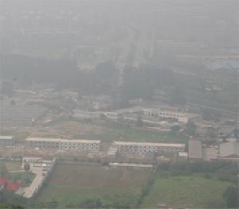
(a) Hazy image

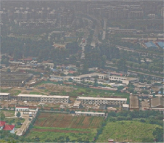
(b) TH model

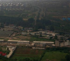
(c) HST model

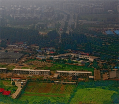
(d) NN model

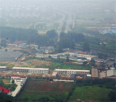
(e) GVPB model

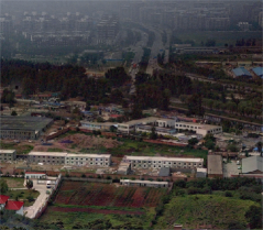
(f) Our model

Figure 1: Dehazed images of five models.

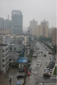
(a) Hazy image

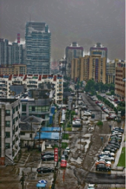
(b) TH model

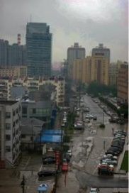
(c) HST model

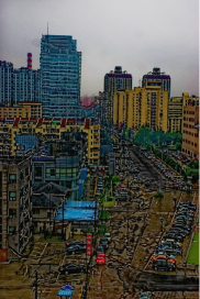
(d) NN model

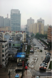
(e) GVPB model

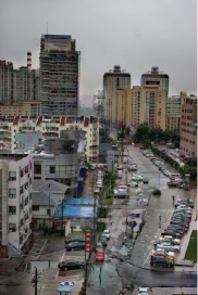
(f) Our model

Figure 2: Dehazed images of five models.

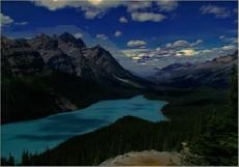
(a) Hazy image

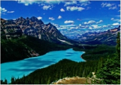
(b) TH model

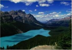
(c) HST model

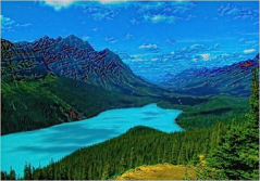
(d) NN model

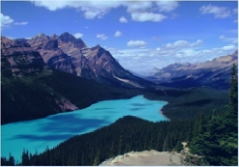
(e) GVPB model

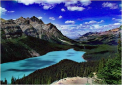
(f) Our model

Figure 3: Dehazed images of five models.

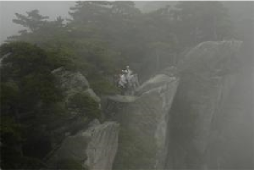
(a) Hazy image

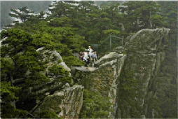
(b) TH model

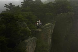
(c) HST model

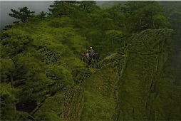
(d) NN model

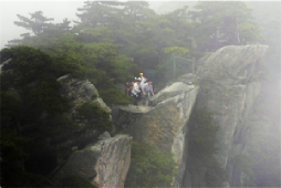
(e) GVPB model

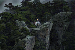
(f) Our model

Figure 4: Dehazed images of five models.

(a) Hazy image

(b) TH model

(c) HST model

(d) NN model

(e) GVPB model

(f) Our model

Figure 5: Dehazed images of five models.

TABLE I: The DIVINE measure.

Figure	TH model	HST model	NN model	GVPB model	Our model
1	69.12939706	55.81779686	76.77106426	27.59361051	51.70167471
2	40.06474732	50.33357282	58.90129268	37.63728444	28.28020355
3	29.5005219	31.67365419	45.48490334	44.623095	31.2784826
4	42.361185	72.74332432	69.26949878	31.99647216	32.35797595
5	34.99726308	31.71468442	36.93765104	58.06464867	34.36637133
6	36.17639358	42.54461789	42.01817754	52.82374224	32.31507553
7	28.25738767	60.46093524	60.4186025	43.18610658	36.35281814
8	33.92395932	37.60110402	44.04815197	48.93872153	25.87425821
9	37.06484625	55.50427775	51.79350658	26.42666981	36.64377696
10	30.40942193	43.31822515	47.75938503	41.11414384	31.5831609
11	42.59571954	71.60576038	62.68818645	22.42739601	46.66527958
12	34.89638836	34.32759134	51.64766252	35.63436032	26.64670178
13	39.73777801	45.69397109	69.62915092	37.56939792	25.76558093
14	44.01071221	37.21166345	55.90721517	33.26285199	32.01531235
15	37.42343679	52.63590884	62.6682146	28.92708829	25.20314234
16	37.36820293	51.08691585	55.30067248	46.37173965	38.32106867
17	37.9279738	55.30492563	52.57334629	29.13674538	32.11836927
18	35.58305551	35.65267976	45.32478858	32.47912919	31.75197257
19	36.22865805	41.2599423	49.21391364	68.02684495	40.57380177
20	30.8861687	102.347466	92.92952377	41.96193037	33.76610649
21	34.18208995	37.6295786	42.56381658	57.82351567	26.45331436
22	21.01591854	40.27551157	43.08234922	42.08302349	34.02561442
23	50.51538052	27.63273381	61.12566397	55.2424206	22.12433037
24	37.19092015	85.19219545	64.07931102	26.615661	55.31714137
25	34.1030265	54.10420943	45.66263991	49.5616121	31.21845141
26	33.93844062	60.76425157	56.8242781	41.99472665	34.63585255
27	26.05382281	37.24908472	46.669687	40.93523376	22.93624267
28	38.88995823	94.43701278	46.3127796	44.19758363	38.66743568
29	26.6411135	49.3601414	47.77859753	34.81849966	29.53926097
30	19.76311212	46.78887595	47.71879282	48.65305246	41.65549273
31	22.12362886	47.5608003	63.05845156	39.41038693	32.53964072
32	27.64718521	63.73911524	51.03978829	37.6896322	29.40947889
33	52.04330222	77.41422594	89.29572858	37.79425201	28.48594041
34	37.80844004	41.8725081	74.21956205	42.0360692	25.22204396
35	33.58540955	33.94907228	56.72764522	35.43403771	24.78363394
36	36.88616844	58.3583864	61.6104566	40.47316711	27.74690379
37	20.89649786	39.94838432	60.51573311	28.70228926	31.75203778
38	46.97055722	74.55770339	77.79395119	40.05672533	28.53793788
39	39.32233495	51.09936157	61.45595098	34.89836413	29.95181701
40	44.3522329	60.50988412	48.60340461	39.35458597	28.23408787
41	35.15425653	63.36065165	61.28628614	42.52254652	36.08010743
42	48.01243888	58.26507293	80.29961957	23.74316958	22.09855608
43	31.1217148	54.78649132	58.45596232	32.89677741	28.65203484
44	50.86545277	59.54538191	73.78767393	33.22594596	30.74138497
45	26.06495856	54.43095529	58.19602786	24.82274303	26.68134416
46	27.32196868	34.37301228	48.13772949	53.17816576	25.59118287
47	60.43678616	66.0121169	66.95232341	20.23993822	33.33448687
48	36.10163092	69.32864735	70.28794576	39.73012258	25.50152289
Average	36.6157	53.1538	58.2256	39.0903	31.7812

References

- [1] A. Beck and M. Teboulle, Fast gradient-based algorithms for constrained total variation image denoising and deblurring problems, IEEE Trans. Image Process., 18(2009), pp. 2419-2434.
- [2] B. Chen and S. Huang, An advanced visibility restoration algorithm for single hazy images, ACM Trans. Multimed. Comput. Commun. Appl., 11(2015).
- [3] L. K. Choi, J. You, and A. C. Bovik, Referenceless prediction of perceptual fog density and perceptual image defogging, IEEE Trans. Image Process., 24(2015), pp. 3888-3901.
- [4] R. Fattal, Single image dehazing, In SIGGRAPH, 2008, pp. 1-9.
- [5] F. Fang, F. Li, and T. Zeng, Single image dehazing and denoising: A fast variational approach, SIAM J. Imaging Sci., 7 (2014), pp. 969-996.
- [6] R. FATTAL, Dehazing Using Color-Lines, ACM Trans. Graph., 34(2014), pp. 13:1-13:14
- [7] A. Galdran, J. Vazquez-Corral, D. Pardo, and M. Bertalm, Enhanced variational image dehazing, SIAM J. Imaging Sci., 8(2015), pp. 1519-1546.
- [8] K. He, J. Sun, and X. Tang, Single image haze removal using dark channel prior, IEEE Trans. Pattern Anal. Mach. Intell., 33 (2011), pp. 2341-2353.
- [9] K. He, J. Sun, and X. Tang, Guided image filtering, IEEE Trans. Pattern Anal. Mach. Intell., 35 (2013), pp. 1397-1409.
- [10] S. Huang, J. Ye, and B. Chen, An advanced single-image visibility restoration algorithm for real-world hazy scenes, IEEE Trans. Ind. Electron, 62(2015), pp. 2962-2972.
- [11] R. KIMMEL, A variational framework for Retinex, Int. J. Comput. Vis., 52(2003), pp. 7-23.
- [12] J. Kopf, B. Neubert, B. Chen, M. Cohen, D. Cohen-Or, O. Deussen, M. Uyttendaele, and D. Lischinski, Deep photo: Model-based photograph enhancement and viewing, ACM Trans. Graph., 27(2008).
- [13] J. Long, Z. Shi, W. Tang, and C. Zhang, Single remote sensing image dehazing, IEEE Geosci. Remote Sensing Lett., 11 (2014), pp. 59-63.
- [14] Y. Lai, Y. Chen, C. Chiou, and C. Hsu, Single-image dehazing via optimal transmission map under scene priors, IEEE Trans. Circuits Syst. Video Technol., 25(2015), pp. 1-14.
- [15] S. G. Narasimhan and S. K. Nayar, Vision and the atmosphere, Int. J. Comput. Vis., 48(2002), pp. 233-254.
- [16] S. G. Narasimhan and S. K. Nayar, Interactive deweathering of an image using physical models, In Workshop on Color and Photometric Methods in Computer Vision, 2003.
- [17] S. Narasimhan and S. Nayar, Contrast restoration of weather degraded images, IEEE Trans. Pattern Anal. Mach. Intell., 25 (2003), pp. 713-724.
- [18] M. K. Ng and W. Wang, A total variation model for Retinex, SIAM J. Imaging Sci., 4 (2011), pp. 345-365.
- [19] K. Nishino, L. Kratz and S. Lombardi, Bayesian defogging, Int J Comput Vis, 98 (2012) pp. 263-278.
- [20] Y. Y. Schechner, S. G. Narasimhan, and S. K. Nayar, Instant dehazing of images using polarization, CVPR, 1(2001), pp. 325-332.
- [21] S. Shwartz, E. Namer, and Y. Y. Schechner, Blind haze separation, CVPR, 2(2006), pp. 1984 - 1991.
- [22] R. Tan, Visibility in bad weather from a single image, CVPR, 2008, pp. 1-8.
- [23] J.-P. Tarel and N. Hautière, Fast visibility restoration from a single color or gray level image, in Proc. IEEE Int. Conf. Comput. Vis., 2009, pp. 2201-2208.
- [24] Y. Wang and C. Fan, Single image defogging by multiscale depth fusion, IEEE Trans. Image Process., 23 (2014), pp. 4826-4837.
- [25] W. Wang and C. He, A variational model with barrier functionals for Retinex, SIAM J. Imaging Sci., 8 (2015), pp. 1955-1980.
- [26] J. Wang, N. He, L. Zhang, and K. Lu, Single image dehazing with a physical model and dark channel prior, Neurocomputing, 149 (2015), pp. 718-728.
- [27] I. Yoon, S. Kim, D. Kim, M.H. Hayes, and J. Paik, Adaptive defogging with color correction in the HSV color space for consumer surveillance system,IEEE Trans. Consum. Electron., 58 (2012), pp. 111-116.
- [28] Q. Zhu, J. Mai, and L. Shao, A fast single image haze removal algorithm using color attenuation prior, IEEE Trans. Image Process., 24(2015), pp. 3522-3533.
- [29] Middleton, Vision through the atmosphere, University of Toronto Press, 1952.
- [30] SK. Dai, JP, Tarel, Adaptive sky detection and preservation in dehazing algorithm, Proc. IEEE International Symposium on Intelligent Signal Processing and Communication Systems, 2015.
- [31] Natural fog-free, foggy, and test images used in FADE:, http://live.ece.utexas.edu/research/fog/fade_defade.html.