Speech vocoding for laboratory phonology

Abstract

Using phonological speech vocoding, we propose a platform for exploring relations between phonology and speech processing, and in broader terms, for exploring relations between the abstract and physical structures of a speech signal. Our goal is to make a step towards bridging phonology and speech processing and to contribute to the program of Laboratory Phonology.

We show three application examples for laboratory phonology: compositional phonological speech modelling, a comparison of phonological systems and an experimental phonological parametric text-to-speech (TTS) system. The featural representations of the following three phonological systems are considered in this work: (i) Government Phonology (GP), (ii) the Sound Pattern of English (SPE), and (iii) the extended SPE (eSPE). Comparing GP- and eSPE-based vocoded speech, we conclude that the latter achieves slightly better results than the former. However, GP – the most compact phonological speech representation – performs comparably to the systems with a higher number of phonological features. The parametric TTS based on phonological speech representation, and trained from an unlabelled audiobook in an unsupervised manner, achieves intelligibility of 85% of the state-of-the-art parametric speech synthesis.

We envision that the presented approach paves the way for researchers in both fields to form meaningful hypotheses that are explicitly testable using the concepts developed and exemplified in this paper. On the one hand, laboratory phonologists might test the applied concepts of their theoretical models, and on the other hand, the speech processing community may utilize the concepts developed for the theoretical phonological models for improvements of the current state-of-the-art applications.

1 Introduction

Speech is a domain exemplifying the dichotomy between the continuous and discrete aspects of human behaviour. On the one hand, the articulatory activity and the resulting acoustic speech signal are continuously varying. On the other hand, for speech communication to convey meaning, this continuous signal must be, at the same time, perceivable as contrastive. Traditionally, these two aspects have been studied within phonetics and phonology respectively. Following significant successes of this dichotomous approach, for example in speech synthesis and recognition, recent decades have witnessed a lot of progress in understanding and formal modelling of the relationship between these two aspects, e.g. the program of Laboratory Phonology (Pierrehumbert et al., 2000) or the renewed interest in the approaches based on Analysis by Synthesis (Hirst, 2011; Bever and Poeppel, 2010). The goal of this paper is to follow these developments by proposing a platform for exploring relations between the mental (abstract) and physical structures of the speech signal. In this, we aim at mutual cross-fertilisation between phonology, as a quest for understanding and modelling of cognitive abilities that underlie systematic patterns in our speech, and speech processing, as a quest for natural, robust, and reliable automatic systems for synthesising and recognising speech.

As a first step in this direction we examine a cascaded speech analysis and synthesis approach (known also as vocoding) based on phonological representations and how this might inform both quests mentioned above. In parametric vocoding speech segments of different time-domain granularity, ranging from speech frames, e.g. in the formant (Holmes, 1973), or articulatory (Goodyear and Wei, 1996; Laprie et al., 2013) domains, to phones (Tokuda et al., 1998; Lee and Cox, 2001), and syllables (Cernocky et al., 1998), are used in sequential processing. In addition to these segments, phonological representations have also been shown to be useful for speech processing e.g. by King and Taylor (2000). In our work, we explore a direct link between phonological features and their engineered acoustic realizations. In other words, we believe that abstract phonological sub-segmental, segmental, and suprasegmental structures may be related to the physical speech signal through a speech engineering approach, and that this relationship is informative for both phonology and speech processing.

The motivation for this approach is two-fold. Firstly, phonological representations (together with grammar) create a formal model whose overall goal is to capture the core properties of the cognitive system underlying speech production and perception. This model, linking subsegmental, segmental, and suprasegmental phonological features of speech, finds independent support in the correspondence between a) the brain-generated cortical oscillations in the `delta' (1-3 Hz), `theta' (4-7 Hz), and faster `gamma' ranges (25-40 Hz), and b) the temporal scales for the domains of prosodic phrases, syllables, and certain phonetic features respectively. In this sense, we may consider phonological representations embodied (Giraud and Poeppel, 2012). Hence, speech processing utilizing such a system might lead to a biologically sensible and empirically testable computational model of speech.

Secondly, phonological representations are inherently multilingual (Siniscalchi et al., 2012). This in turn has an attractive advantage in the context of multilingual speech processing in lessening the reliance on purely phonetic decisions. The independence of the phonological representations from a particular language on the one hand and the availability of language specific mapping between these representations and the acoustic signal through speech processing methods on the other hand, offer (we hope) a path towards a context-based interpretation of the phonological representation that is grounded in phonetic substance but at the same time abstract enough to allow for a more streamlined approach to multilingual speech processing.

In this work, we propose to use the phonological vocoding of Cernak et al. (2015) and other advances of speech processing for testing certain aspects of phonological theories. We consider the following phonological systems in this work:

• The Government Phonology (GP) features (Harris and Lindsey, 1995) describing sounds by fusing and splitting of 11 primes.

• The Sound Pattern of English (SPE) system with 13 features established from natural (articulatory) features (Chomsky and Halle, 1968).

• The extended SPE system (eSPE)  (Yu et al., 2012; Siniscalchi et al., 2012) consisting of 21 phonological features.

Having trained phonological vocoders for the three phonological models of sound representation, we describe several application examples combining speech processing techniques and phonological representations. Our primary goal is to demonstrate the usefulness of the analysis by synthesis approach by showing that (i) the vocoder can generate acoustic realizations of phonological features used by compositional speech modelling, (ii) speech sounds (both individual sounds not seen in training and intelligible continuous speech) can be generated from the phonological speech representation, and (iii) the testing of hypotheses relating phonetics and phonology is possible; we test the hypothesis that the best phonological speech representation achieves the best quality vocoded speech, by evaluating the phonological features in both directions, recognition and synthesis, simultaneously. Additionally, we compare the segmental properties of the phonological systems, and describe results and advantages of experimental phonological parametric TTS system. To preview, conventional parametric TTS can be described as phonetic, i.e., phonetic and other linguistic and prosodic information is used in the input labels. On the other hand, our proposed system can be described as phonological, i.e., only information based on phonological representation is used as input. This allows, for example, for generation of any new speech sounds.

The structure of the paper is as follows: the phonological representations used in this work are introduced in Section 2. Section 3 introduces speech vocoding based on phonological speech representation. Section 4 describes the experimental setup. The application examples of the proposed platform (along with the experiments and results) are shown in Section 5. Finally the conclusions follow in Section 6.

2 Phonological systems

Phonology is construed in this work as a formal model that represents cognitive (subconscious) knowledge of native speakers regarding the systematic sound patterns of a language. The two traditional components of such models are i) system primitives, that is, the units of representation for cognitively relevant objects such as sounds or syllables, and ii) a set of permissible operations over these representations that is able to generate the observed patterns. Naturally, these two facets are closely linked and inter-dependent. In this paper we focus on the theory of representation.

2.1 Segmental representations

The minimal unit of meaning contrast, i.e. cognitive relevance, is assumed to be the phoneme. In the tradition of Jakobson and Halle (1956) and Chomsky and Halle (1968), phonemes are assumed to consist of feature bundles. In the former model of Jakobson and Halle (1956), 12 basic perceptual-acoustic domains (e.g. acute-grave, or compact-diffuse) define the space for characterising all the phonemes. The model uses polar opposites for these 12 continua, which are necessarily relational, and thus language-specific. Hence, a vowel characterised as, e.g. ‘grave’ in one language might be phonetically different from the same grave vowel in another language since their grave quality might be at a different point of the acute-grave continuum. The latter system of Chomsky and Halle (1968), known also as SPE, differed from the former system of Jakobson and Halle (1956) in two fundamental aspects relevant for this paper. First, it took the articulatory production mechanism as the underlying principle of phoneme organisation; hence, in their 13 basic binary features, we talk about the position (or activity) of the active articulators rather than percepts they create. Second, SPE assumed that the flat, unstructured binary feature specifications are language independent and characterise the set of possible phonemes in languages of the world.

The developments of phonological theory after SPE focused on both the theory of representations as well as the operations. The most relevant for this paper are proposals for establishing the non-linear nature of phonological representations, i.e., the fact that individual features are not strictly linked to the linear sequence of sounds but may span greater domains or occupy independent non-overlapping tiers. These proposals started with the representation of lexical tones (Leben, 1973; Goldsmith, 1976), continued with the featural geometry approach (Sagey, 1986; Clements and Hume, 1995) and received novel formal treatments in the theories of Dependency and Government Phonology (GP), e.g. Kaye et al. (1990), Harris (1994). These latter approaches posit the so called primes, or basic elements, that are monovalent (c.f. binary SPE features). For example, there are four basic resonance primes commonly labelled as A, U, I, and @; the first three denoting the peripheral vowel qualities [a], [u] and [i] respectively, the last one describing the most central vowel quality of schwa. English [i:] would correspond to the I prime while [e] results in fusing the I and A primes. In addition to these `vocalic' primes, GP proposes the `consonantal' primes ?, h, H, N, denoting closure, friction, voicelessness and nasality respectively. To account for the observed variability in inventories (e.g. English has 20 contrastive vowels and thus 20 different phonetic representations for them), phonetic qualities, and types of phonological behaviour, the phoneme representations based on simple primes become insufficient. The solution, given the name of the framework, is that some elements can optionally be heads and govern the presence or realisation of other (dependent) elements.

These developments established the relevance of the internal structure of phonological primitives and their hierarchical nature. Furthermore, the non-linear nature of phonological representations became the accepted norm for formal theories of phonology. Importantly, while the SPE-style features were assumed to require the full interpretation of all features for a surface phonetic realisation of a phoneme, the primes of GP are assumed to be interpretable alone despite their sub-phonemic nature. Harris and Lindsey (1995) call this GP assumption the autonomous interpretation hypothesis.

This hypothesis, and its testing, is at the core of our approach. One of the goals of this work is to provide an interpretation for sub-phonemic representational components of phonology that is grounded in the acoustic signal.

2.2 Representing CMUbet with SPE and GP

To characterise the phoneme inventory of American English in the SPE and the GP frameworks, we have adopted the approach of King and Taylor (2000) with some modifications. We use the reduced set of 39 phonemes in the CMUbet system. The major difference regarding the SPE-style representations is our addition of a [rising] feature used to differentiate diphthongs from monophthongs. In the original SPE framework, this difference was treated with the [long] feature and the surface representation of diphthongs was derived from long monophthongs through a rule. Given the absence of the `rule module' in our approach to synthesis, we opted for a unified feature specification of the full vowel inventory of American English using the added feature. This allowed for diphthongs to form a natural class with vowels rather than with glides [j, w] as in King and Taylor (2000). Additional minor adjustments assured the uniqueness of a feature matrix for each phoneme. The full specification of all 39 phonemes with 14 binary features is shown in Table 2.

The set of GP-style specification for English phonemes can be seen in Table 1. Again, we followed King & Taylor, mostly in formalizing headedness with pseudo-features, which allows for GP phoneme specifications that are comparable to SPE. Additionally, the vowel specifications differ somewhat from King & Taylor stemming from our effort to approximate the phonetic characteristics of the vowels, and the differences among them, as closely as possible. For example, if the back lax [U] is specified with E, the same was employed for the front lax [I], or, the front quality of [æ] was formalized with A heading I compared to King & Taylor's formalism with only non-headed A.

3 Phonological vocoding

Both SPE and GP phonological systems represent a phone by a combination of phonological features. For example, a consonant [j] is articulated using the mediodorsal part of the tongue [+Dorsal], in the mediopalatal part of the vocal tract [+High], generated with simultaneous vocal fold vibration [+Voiced]. These three features then comprise the phonological representation for [j] in the SPE system.

Cernak et al. (2015) have recently designed a phonological vocoder for a low bit rate parametric speech coding as a cascaded artificial neural network composed of speech analyser and synthesizer that use a shared phonological speech representation. Figure 1 shows a sequential processing of the vocoding, briefly introduced in the following text.

3.1 Phonological analysis

Figure 1: The process of the phonological vocoding. The speech signal is internally represented by phonological posterior probabilities $\mathbf{z}_{n}$, consisting of $K$ phonological posteriors per $n$-th frame). The DNN-based synthesizer generates speech parameters – line spectral pairs (LSPs) and source parameters for LPC speech re-synthesis.

Phonological analysis starts with speech analysis that turns speech samples into a sequence of acoustic feature observations $X=\{\mathbf{x}_{1},\ldots,\mathbf{x}_{n},\ldots,\mathbf{x}_{N}\}$ where $N$ denotes the number of frames in the speech signal. Conventional cepstral coefficients can be used in this speech analysis step. Then, a bank of phonological analysers realised as neural network classifiers converts the acoustic feature observation sequence $X$ into a sequence of vectors $Z=\{\mathbf{z}_{1},\ldots,\mathbf{z}_{n},\ldots,\mathbf{z}_{N}\}$ where a vector $\mathbf{z}_{n}=[z_{n}^{1},\ldots,z_{n}^{k},\ldots,z_{n}^{K}]^{T}$ consists of $K$ phonological feature posterior probabilities, called hereinafter the phonological posteriors. The posteriors $z_{n}^{k}$ are probabilities that the $k$-th feature occurs (versus does not occur), and they compose the information which is transferred to the synthesizer's side in order to synthesize speech as described in the next subsection. These posteriors can be optionally pruned (compressed) if there is need for reducing the amount of transferred information (i.e. reducing the bit rate). For example, the binary nature of the phonological features considered by Cernak et al. (2015) allowed for using binary values of the phonological features instead of continuous values, which resulted only in minimal perceptual degradation of speech quality.

There are two main groups of the phonological features:

• segmental: phonological features that define the phonetic surface of individual sounds,

• supra-segmental: phonological features at the timescales of syllables and feet (including a single stressed syllable and one or more unstressed ones.

In this work, we focus on the segmental phonological features and leave the supra-segmental for future research.

3.2 Phonological synthesis

The phonological synthesizer is based on a Deep Neural Network (DNN) that learns the highly-complex regression problem of mapping posteriors $z_{n}^{k}$ to the speech parameters. More specifically, it consists of two computational steps. The first step is a DNN forward pass that generates the speech parameters, and the second one is a conversion of the speech parameters into the speech samples. The second stage of synthesis is based on an open-source LPC re-synthesis with minimum-phase complex cepstrum glottal model estimation (Garner et al., 2015). The modelled speech parameters are thus:

• $\mathbf{p}_{n}$: static Line Spectral Pairs (LSPs) of 24th order plus gain,

• $\log(\mathbf{r}_{n})$: a Harmonic-To-Noise (HNR) ratio,

• and $\mathbf{t}_{n}$, $\log(\mathbf{m}_{n})$: two glottal model parameters – angle and magnitude of a glottal pole, respectively.

The generated speech parameter vectors – $\mathbf{p}_{n}$, $\mathbf{t}_{n}$, $\log(\mathbf{r}_{n})$ and $\log(\mathbf{m}_{n})$ for the $n$-th frame – from the first computational step are smoothed using dynamic features and pre-computed (global) variances (Tokuda et al., 1995), and formant enhancement (Ling et al., 2006) is performed to compensate for over-smoothing of the formant frequencies. The speech samples are finally generated frame by frame followed with overlap-and-add. LPC re-synthesis can be done either with synthesised or original pitch features.

4 Experimental setup for laboratory phonology

In this section, the experimental protocol of the phonological analysis and synthesis is described. In Table 1, the data used in these experiments are presented. The analyser is trained on the Wall Street Journal (WSJ0 and WSJ1) continuous speech recognition corpora (Paul and Baker, 1992). The si_tr_s_284 set of 37,514 utterances was used, split into 90% training and 10% cross-validation sets. The synthesizer is trained and evaluated on an English audiobook ``Anna Karenina'' of Leo Tolstoy, that is around 36 hours long. Recordings were organised into 238 sections, and we used sections 1–209 as a training set, 210–230 as a development set and 231–238 as a testing set. The development and testing sets were 3 hours and 1 hour long, respectively.

Table 1: Data used for training the phonological analysis and synthesis.

Use of data Database Set/Section Size Analyser (train. set) WSJ si_tr_s_284 33.765 (utts) Analyser (cross-val. set) WSJ si_tr_s_284 3.749 (utts) Synthesizer (train. set) Tolstoy 1-209 36 (hours) Synthesizer (dev. set) Tolstoy 210-230 3 (hours) Synthesizer (test set) Tolstoy 231-238 1 (hour)

4.1 Phonological analysis

The analyser is based on a bank of phonological analysers realised as neural network classifiers – multilayer perceptrons (MLPs) – that estimate phonological posteriors. Each MLP is designed to classify a binary phonological feature.

First, we trained a phoneme-based automatic speech recognition system using Perceptual Linear Prediction (PLP) features. The phoneme set comprising of 40 phonemes (including ``sil'', representing silence) was defined by the CMU pronunciation dictionary. The three-state, cross-word triphone models were trained with the HTS variant (Zen et al., 2007) of the HTK toolkit on the 90% subset of the si_tr_s_284 set. The remaining 10% subset was used for cross-validation. We tied triphone models with decision tree state clustering based on the minimum description length (MDL) criterion (Shinoda and Watanabe, 1997). The MDL criterion allows an unsupervised determination of the number of states. In this study, we obtained 12,685 states and modeled each state with a Gaussian mixture model (GMM) consisting of 16 Gaussians.

4.1.1 Alignment

A bootstrapping phoneme alignment was obtained using forced alignment with cross-word triphones. The bootstrapping alignment was used for the training of the bootstrapping MLP, using as the input 39 order PLP features with the temporal context of 9 successive frames, and a softmax output function. The architecture of the MLP, 3-hidden layers $351\times 2000\times 500\times 2000\times 40$ (input $351=39\times 9$ and output 40 is the number of phonemes), was determined empirically. Using a hybrid speech decoder fed with the phoneme posteriors, the re-alignment was performed. After two iterations of the MLP training and re-alignment, the best phoneme alignment of the speech data was obtained. This re-alignment increased the cross-validation accuracy of the MLP training from 77.54% to 82.36%.

4.1.2 Training of the bank of phonological analysers

The representation given in A was used to map the phonemes of the best alignment to phonological features for the training of the analysers. $K$ analysers were trained with the frame alignment having two output labels, the $k$-th phonological feature occurs for the aligned phoneme or not. The analysis MLPs were finally trained with the same input features as used for the alignment MLP, and the same network architecture except for 2 output units instead of 40. The output that encodes the phonological feature occurrence is used as the vector of phonological posteriors $\mathbf{z}_{n}$.

Tables 2, 3, and 4 show classification accuracies at frame level of the GP, SPE and eSPE MLPs for the ``feature occurs'' output, respectively. The accuracies are reported for the training and cross-validation sets (see Table 1 for data sets definition). The analysers performances are high, with an average cross-validation training accuracy of 95.5%, 95.6% and 96.3%, respectively. It is interesting that as the number of phonological features increases, the classification accuracy also increases. The reason might be that a more precise representation of the phonological features is used (the maps given in A).

Table 2: Classification accuracies (%) of the GP prime analysers at frame level on cross-val. set of si_tr_s_284 set.

Primes Accuracy (%) Primes Accuracy (%) train cv train cv A 92.3 91.7 a 97.9 97.6 I 94.9 94.6 i 96.1 96.4 U 94.4 94.1 u 97.5 97.7 E 92.6 91.9 H 95.4 95.0 S 95.2 94.7 N 98.2 98.1 h 95.9 95.4 sil 99.0 98.9

Table 3: Classification accuracies (%) of the SPE analysers at frame level on cross-val. set of si_tr_s_284 set.

Phonological Accuracy (%) Phonological Accuracy (%) features train cv features train cv vocalic 96.0 95.8 round 97.8 97.7 consonantal 94.5 93.9 tense 94.8 94.1 high 94.8 94.4 voice 94.6 94.4 back 93.9 93.4 continuant 95.6 95.2 low 97.4 97.1 nasal 98.1 98.0 anterior 94.4 94.0 strident 97.8 97.6 coronal 94.3 93.9 sil 99.0 98.9

Table 4: Classification accuracies (%) of the eSPE analysers at frame level on cross-val. set of si_tr_s_284 set.

Phonological Accuracy (%) Phonological Accuracy (%) features train cv features train cv vowel 94.7 94.3 low 97.5 97.2 fricative 97.3 97.0 mid 94.5 94.0 nasal 98.2 98.1 retroflex 98.6 98.4 stop 96.7 96.4 velar 98.9 98.8 approximant 97.2 96.9 anterior 94.8 94.3 coronal 94.8 94.4 back 94.2 93.8 high 94.6 94.2 continuant 95.8 98.4 dental 99.3 99.2 round 95.3 94.9 glottal 99.7 99.7 tense 91.4 90.7 labial 97.6 97.4 voiced 95.2 94.9

4.2 Phonological synthesis

4.2.1 Training

The speech signals from the training and cross-validation sets of the Tolstoy database, down-sampled to 16 kHz, framed by 25-ms windows with 10-ms frame shift, were used for extracting both DNN input and output features. The input features, phonological posteriors $\mathbf{z}_{n}$, were generated by the phonological analyser trained on the WSJ database. The temporal context of 11 successive frames resulted in input feature vectors of 132 ($12\times 11\times 1$), 165 ($15\times 11\times 1$) and 231 ($21\times 11\times 1$) dimensions, for the GP, SPE and eSPE schemes, respectively. The output features, the LPC speech parameters, were extracted by the Speech Signal Processing (SSP) python toolkit. We used static speech parametrization of 29th order along with its dynamic features, altogether of 87th order.

Cepstral mean normalisation of the input features was applied before DNN training. The DNN was initialised using $(K\times 11)\times 1024\times 1024\times 1024\times 1024$ Deep Belief Network pre-training by contrastive divergence with 1 sampling step (CD1) (Hinton et al., 2006). The 4 hidden layers DNN with a linear output function was then trained using a mini-batch based stochastic gradient descent algorithm with mean square error cost function of the KALDI toolkit (Povey et al., 2011). The DNN had 3.4 million parameters.

4.2.2 Synthesis

The test set of the Tolstoy database was used for the synthesis. There are three options to generate a particular speech sound: (i) by $Z$ inferred from the speech, (ii) by $Z$ inferred from the text, or (iii) by compositional speech modelling. In the two first cases, we refer to this generation as network-based. The speech parameters generated by the forward DNN pass are smoothed using dynamic features and pre-computed (global) variances, and formant enhancement is performed to mitigate over-smoothing of the formant frequencies.

In the latter case, speech sounds are generated using compositional phonological speech models, introduced next in Section 5.1. Briefly, we set a single phonological feature as an active input and the rest are set to zeros. This generates an artificial audio sound that characterises the input phonological feature. Then, the speech sound is generated by the composition (audio mixing) of the particular artificial audio sounds. We refer to this process as compositional-based. We wanted a) to show that compositional phonological speech modelling is possible, b) to test the suitability of speech sound synthesis without the DNN, i.e., only by mixing the artificial phonological sound components, and c) to allow the reader to experiment with the sound components that are embedded in this manuscript.

5 Application examples for laboratory phonology

In this section we show how to use the phonological vocoder, described in Section 4, a) for compositional phonological speech modelling (Section 5.1), b) for a comparison of phonological systems (Section 5.2) and c) as a parametric phonological TTS system (Section 5.3.2).

5.1 Compositional phonological speech models

Virtanen et al. (2015) investigate the constructive compositionality of speech signals, i.e., representing the speech signal as non-negative linear combinations of atomic units (``atoms''), which themselves are also non-negative to ensure that such a combination does not result in subtraction or diminishment. The power of the sum of uncorrelated atomic signals in any frequency band is the sum of the powers of the individual signals within that band. The central point is to define the sound atoms that are used as the compositional models.

Following this line of research, we hypothesise that the acoustic representation of the phonological features, produced by a phonological vocoder, forms a set of speech signal atoms (the phonological sound components) that define the phones. We call these sound components phonological atoms. It is possible to generate the atoms for any phonological system.

$$Z=\left(\begin{array}[]{*4{c}}\leavevmode\hbox to11.67pt{\vbox to13.11pt{\text{[drawing]}}}&0&0&0\\ 0&1&0&0\\ 0&0&1&0\\ \leavevmode\hbox to11.67pt{\vbox to13.11pt{\text{[drawing]}}}&0&0&1\end{array}\right)\leavevmode\hbox to12.87pt{\vbox to14.31pt{\text{[drawing]}}}$$

Figure 2: Generation of a sound of the first phonological atom. The artificial phonological representation, the identity matrix, is for illustration of size 4. The phonological synthesis DNN generates the speech parameter vectors: the 24th order line spectral pairs, the harmonic to noise ratio, and the angle and magnitude of a glottal pole. The speech parameters are then re-synthesized by LPC re-synthesis.

Given our hypothesis above (that these phonological atoms form a set of acoustic templates that might be taken to define speech acoustic space), we defined artificial representations $Z=\{\mathbf{z}_{1},\ldots,\mathbf{z}_{k},\ldots,\mathbf{z}_{K}\}$ as the identity matrix $I_{K}$ of size $K\times K$. Each column represents a phonological atom, and its speech samples are generated as described in Section 3.2, and illustrated in Figure 2.

Thus, we can listen to the sounds of individual phonological features. As an example, Table 1 in B demonstrates recordings of phonological features of the GP system. We generated these phonological sounds also for the SPE and eSPE phonological systems and used all of them in the following experiments.

Finally, the composition of the speech sounds, the phones, driven by the canonical phone representation, is done as follows:

$$\mathbf{y}_{n}=\frac{1}{S}\sum_{s=1}^{S}w_{n}^{s}z_{n}^{s},$$ (1)

where $\mathbf{y}_{n}$ is a composition of $S$ (a particular subset of $K$ phonological features) phonological atoms, and $w_{n}^{s}$ are weights of the composition. The weights are a-priori mixing coefficients not investigated closer in this work; we used them as constants with the value of 1.

The presented compositional speech sound generation is context-independent and generates the middle parts of the phones.

5.2 Comparison of the phonological systems

We start with context-independent vocoding in Section 5.2.1, i.e., the vocoding of isolated speech sounds, and continue with context-dependent vocoding in Section 5.2.2.

5.2.1 Context-independent vocoding

The aim of this subsection is to objectively evaluate the phonological systems in respect to context-independent vocoding, i.e., the ability of phonological systems to produce isolated speech sounds. In order to achieve this, instead of inferring the posteriors from the speech, we generated the canonical phonological posteriors, i.e., we used only the features that represent the specific isolated phones (rows of Tables 1, 2, and 3). Original speech, manually phonetically labelled 76 utterances from the audiobook test set, was used as the reference for the comparison. Having the phoneme boundaries, we extracted 25ms windows from the central (stationary) part of the phones, to obtain human spoken acoustic references.

Finally, we used the Mel Cepstral Distortion (MCD) (Kubichek, 1993) to calculate perceptual acoustic distances between the $P$ vocoded phones and the spoken references, a distance matrix $D_{vocoded}$. The MCD values are in dB and higher values represent more confused phones. In order to visually compare confusions introduced by the different phonological representations, we normalised $D_{vocoded}$ by distances between the spoken references only, a distance matrix $D_{natural}$, resulting into the distance matrix $D_{norm}$. The definitions of the distance matrices are as follow:

$$D_{natural} =[D_{1},\ldots,D_{p},\ldots,D_{P}]$$ (2)

$$D_{p} =\mathbf{1}+\left(\mathbf{1}-\left(\max\left(N_{p}\right)\mathbf{1}-N_{p}\right)\oslash\left(\max\left(N_{p}\right)\mathbf{1}-\min\left(N_{p}\right)\mathbf{1}\right)\right)$$ (3)

$$D_{norm} =D_{vocoded}\odot D_{natural}$$ (4)

where $\mathbf{1}$ is the all ones vector of dimension $P$, $N_{p}$ is a vector of MCDs values between a phoneme $p$ and all other phonemes, and $D_{p}$ are the scaled values between $1$ and $2$, by $1$ referring to the minimal distance (no confusion). Operator $\odot$ stands for element-wise matrix multiplication (the Hadamard product), $\oslash$ stands for element-wise matrix division. For illustration, Figure 3 shows the distance matrix $D_{natural}$. To better visualise the contrast of the distances around 1, the maximum value of the colour map is set to 1.5 (i.e., the distances above 1.5 are also white).

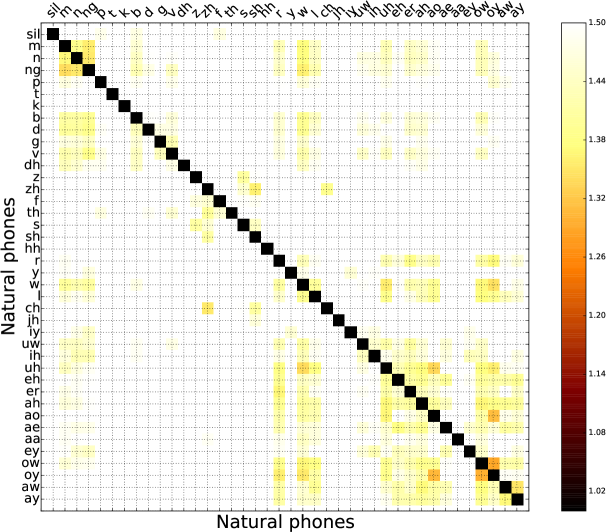
Figure 3: Scaled distance matrix $D_{natural}$ of the spoken acoustic references.

Figures 4, 5 and 6 show normalised distance matrices $D_{norm}$ of vocoded context-independent phones and the spoken acoustic references of the same speaker, for the GP, SPE and eSPE phonological systems, respectively. The diagonal elements of the distance matrices represent an acoustical distance (dissimilarity) of vocoded and spoken phones. If the phonological features represent speech well, the matrices show only strong diagonals. Missing diagonal values imply greater distance between spoken and vocoded phones, and might be caused by erroneous assignment of phonological features to phonemes (the maps given in A) during the training of the phonological analysis.

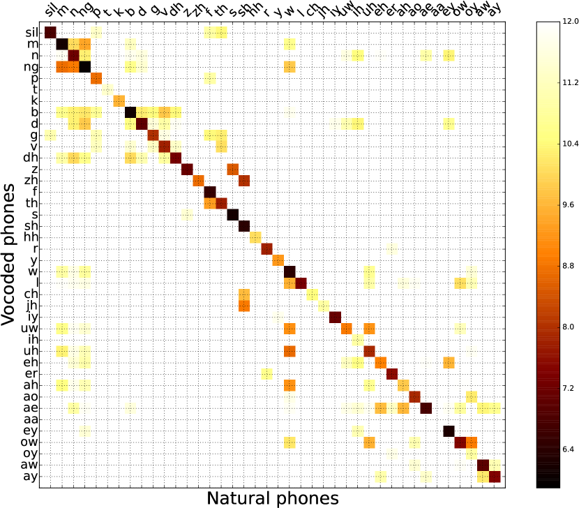
(a) Network-based

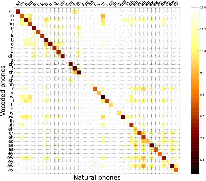
(b) Compositional-based

Figure 4: $D_{norm}$ of GP vocoded and spoken phones.

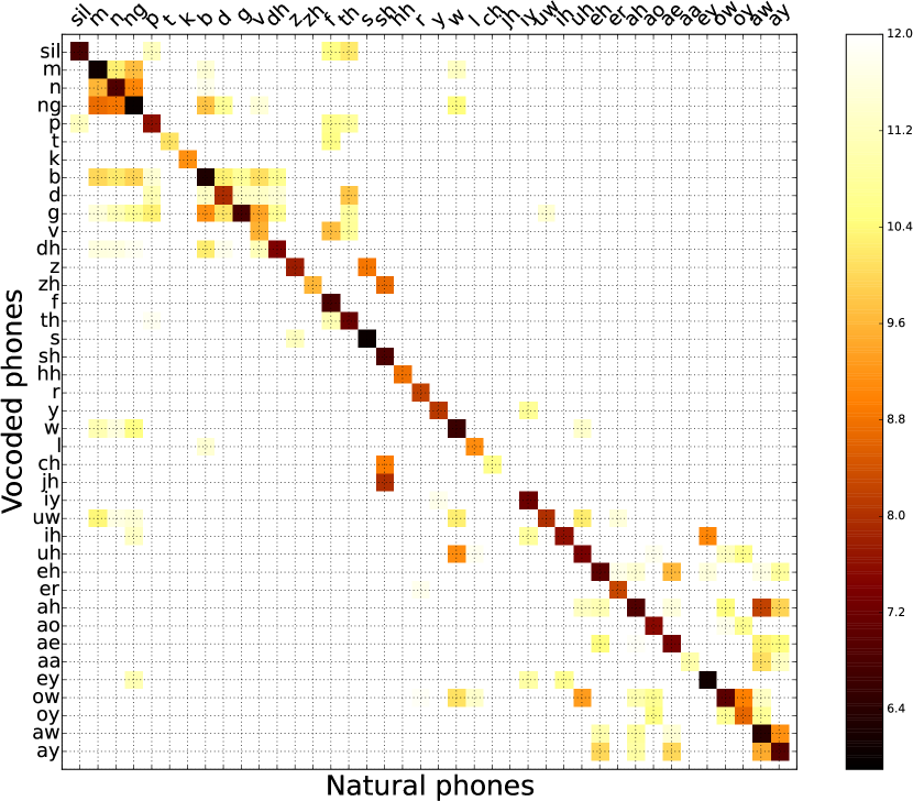
(a) Network-based

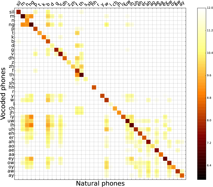
(b) Compositional-based

Figure 5: $D_{norm}$ of SPE vocoded and spoken phones.

(a) Network-based

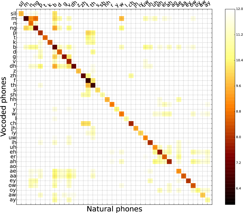
(b) Compositional-based

Figure 6: $D_{norm}$ of eSPE vocoded and spoken phones.

The figures show two aspects of the evaluation. In the first, the distance matrices of (a) the network-based and (b) the compositional-based phonological synthesis are shown. The network- and compositional-based synthesis differ in the way features are combined. In the first case, the DNN inputs are combined so as to generate specific phones. In the second case, phonological atoms of the specific phone are combined in order to generate compositional phones. We can therefore consider this as two different evaluation metrics, hypothesising that both contribute partially to a final evaluation. In both cases, the ideal performance is to have dark diagonals, i.e., the lowest acoustic distance between the spoken reference and vocoded phones. We consider the deviations from the ideal performance as the errors and this allows us to search for patterns in these errors. Table 5 shows the averages of the diagonal values of the distance matrices.

Table 5: The average MCD values given in [dB] of the diagonals of the distance matrices shown in Figures  4, 5 and 6.

System Network Compositional GP 8.12 8.67 SPE 7.79 8.77 eSPE 7.87 8.79

For all three phonological systems, the results of compositional-based context-independent vocoding show greater errors (i.e., higher values in Table 5) than the ones of network-based vocoding. This might be caused by the fact that the composition of the phonological atoms is a linear operation (as shown in Section 5.1), and it is an approximation to a non-linear function that is modelled by network-based phonological synthesis. Additionally, the types of reported errors in the network-based vocoding that are missing in the compositional-based one make sense phonetically. For example, in the left panel of Figure 4(a), phonetically very similar [Z], [S], [dZ], [tS] with voicing and closure being highly context dependent have also smaller acoustic distances. Nevertheless, compositional-based vocoding tends to produce smaller errors in all three frameworks. For example, while [D] in the left panel of Figure 4(a) has smaller acoustic distances with nasals, voiced plosives and [v], the right panel shows only smaller distances only with labials.

In the second aspect of the evaluation, the three phonological systems (GP, SPE and eSPE) are compared among themselves using network-based synthesis. In Figures 4(a), 5(a), and 6(a), we see different error patterns. In all three phonological systems the biggest errors are shown with the nasals [m n N]. GP in addition produces errors in the consonants and vowels, such as for nasals. SPE seems to represent speech better, namely for vowel [A] and glide [w], and suppresses most of the vowel-consonant errors. On the other hand, it fails with proper [dZ] vocoding. We speculate that phone frequency in the evaluation data may be one of the causes of these errors; for example, the phone [dZ] was the least frequent one in our data. Finally, according to our data, eSPE further improves on the SPE speech representation. It generates fewer errors in the vowel space, and also in the consonant space, for example in the voiced stops class [b d g].

5.2.2 Context-dependent vocoding

The previous experiment evaluated the vocoding of the isolated sounds, using canonical posteriors $\mathbf{z}_{n}$. We continued with the evaluation of continuous speech vocoding using $\mathbf{z}_{n}$ inferred from the reference speech signals. Network-based phonological synthesis was used for the following experiments.

In this evaluation, we were interested if the segmental errors found in context-independent vocoding impact the context-dependent vocoding. We employed a subjective evaluation listening test (Loizou, 2011), suitable for comparing two different systems. In this pair-wise comparison test, listeners were presented with pairs of samples produced by two systems and for each pair they indicated their preference. The listeners also were presented with the choice of ``no preference'', when they couldn't perceive any difference between the two samples. The material for the test consisted of 16 pairs of sentences such that one member of the pair was generated using the GP-based vocoder and the other member was generated using the eSPE-based vocoded speech. Random utterances from the test set of the Tolstoy database were used to generate the vocoded speech. We chose these two systems because they displayed the greatest differences in context-independent results. The subjects for the listening test were 37 listeners, roughly equally pooled from experts in speech processing on the one hand, and completely naive subjects on the other hand. The subjects were presented with pairs of sentences in a random order with no indication of which system they represented. They were asked to listen to these pairs of sentences (as many times as they wanted), and choose between them in terms of their overall quality. Additionally, the option ``no preference'', was available if they had no preference for either of them. To decrease the demands on the listeners, we divided the material into two different sets, each consisting of 8 paired sentences randomly selected from the test set. The first set was presented to 19 listeners, and the second set to 18 different listeners.

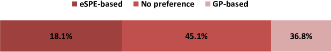
Figure 7: Subjective preference score (%) between the GP-based and the eSPE-based vocoded speech

In Figure 7 the results of the subjective listening test for the GP and eSPE phonological systems, are shown. As can be seen, the eSPE-based phonological vocoder outperforms the GP one by 36.8% compared with 18.1% preference score. Even though there is a preference of the listeners towards the eSPE-based system (double preference percentage), it is clearly shown that with a very high percentage, 45%, the two systems are perceived by the listeners as having the same overall quality (no preference). It should be pointed out that a $t$-test confirmed that this difference between the GP-based and eSPE-based phonological vocoders is statistically significant ($p<0.01$).

We hypothesize that the preference for eSPE is linked to greater perceptual clarity of individual phones. Subsequent auditory and visual analyses of the sample sentences and their generated acoustic signals suggest that eSPE sentences displayed longer closures for plosives, stronger plosive releases, and also slightly greater disjunctures at some word boundaries. These features correspond to a decreased overlap of sounds, i.e. decreased coarticulation, commonly present in hyper-articulated or clearly enunciated speech.

5.3 Experimental parametric phonological TTS

In this section we show how compositional phonological speech models could be combined to generate arbitrary speech sounds, and how to synthesise continuous speech from the canonical phonological representation.

5.3.1 Generation of sounds from unseen language

In this experiment, we arbitrarily selected the GP system to demonstrate the phonological composition of new speech sounds. Harris (1994) claims that fusing and splitting of primes accounts for phonological description of the sound. We selected the phonological rule number 29 [I, U, E] $\rightarrow$ y, and [A, I, U, E] $\rightarrow$ œ, of Harris (1994) and tried to synthesise non-English sounds by the composition of involved phonological atoms. According to Section 5.1, we claim that new sounds can be generated by time-domain mixing of the corresponding atoms $\mathbf{a}^{s}$. Table 2 demonstrates the synthesis of standard German sounds [y] and [œ] from English phonological atoms $\mathbf{a}^{s}$, generated as in Eq. 1. For $w_{n}^{s}=1$, it can be done easily with available free tools, e.g.:

• ] : sox -m I.wav U.wav E.wav y.wav

• ] : sox -m A.wav I.wav U.wav E.wav oe.wav

We performed a formant analysis of all phonological atoms, and concluded that they contain the same number of formants as human speech sounds (i.e., 4 in the 5 kHz bandwidth). In addition, the combined sounds also contain the proper number of formants. The first two formants play a major perceptual role in distinguishing different English vowels (Ladefoged and Johnson, 2014), and Figure 8 shows F1 and F2 of [œ] phone from Table 2. The mean value of the first formant of the natural [œ] takes values between 509 Hz (Gendrot and Adda-Decker, 2005) and 550 Hz (Pätzold and Simpson, 1997). The mean values of the second formant of the natural [œ] takes values between 1650 Hz and 1767 Hz. The average F1 of synthesized [œ] is 559 Hz and F2 is 1917 Hz. Those numbers are slightly higher than average population numbers, however, they may be related to our female speaker used in the training of the phonological synthesis.

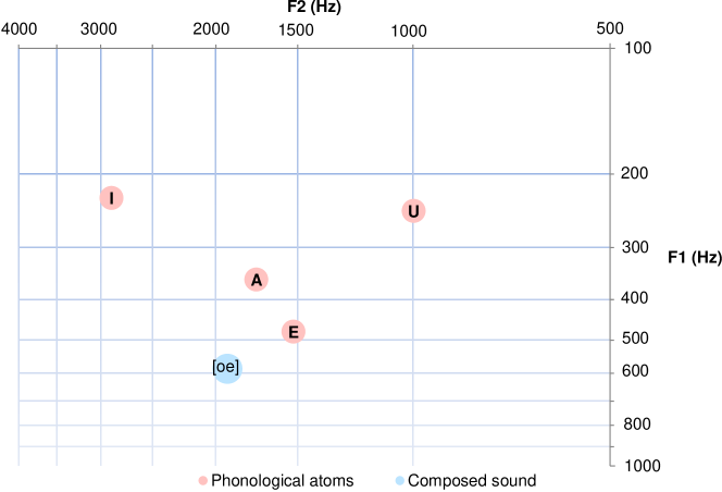
Figure 8: First two formants of involved phonological atoms and their composition – a phone [œ].

The results of this experiment support the hypothesis mentioned in Section 5.1, that phonological atoms may define the phones. In addition, Section 5.2.1 demonstrated that compositional-based phonological synthesis works well also for the SPE and eSPE phonological systems.

Figure 9: Phonological TTS synthesis. Speech parameters, the speech line spectral pairs LSPs and source parameters, are generated by the DNN. Speech samples are generated by subsequent LPC re-synthesis.

5.3.2 Continuous speech synthesis

The composition of Eq. 1 represents a static mixing of $S$ phonological atoms, i.e., it cannot be applied to model co-articulation. To include co-articulation into the synthesis, the phonological synthesizer has to be used. As it was trained with the temporal context of 11 successive frames, around 50 ms before and 50 ms after the current processing frame, it learnt how speech parameters change with trajectories of the phonological posteriors.

Experimental parametric phonological TTS can be designed by a simplistic text processing front end: input text transformed into the phonemes using a lexicon, and the phonemes transformed to phonological features using maps given in A. Figure 9 shows the TTS process with the phonological synthesis. The binary phonological representation to be synthesized is obtained again from the canonical phone representation.

To demonstrate the potential of our parametric phonological TTS system, we randomly selected three utterances from a slt subset of the CMU-ARCTIC speech database (Kominek and Black, 2004), and used their text labels to generate continuous speech. Specifically, we used the phoneme symbols along with their durations from the forced-aligned full-context labels provided with the database, and mapped it to the phonological representation. Then we synthesised the sentences using the already trained phonological synthesizers as described in Section 4.2.1.

Table 3 lists recordings that demonstrates speech synthesis from the phonological speech representation. The example a0453 illustrates how the phonological vocoder learns the context. Figure 10 visualises the generated GP and eSPE examples. The phoneme sequence of the first word is [eI t i n], while the synthesised sequences using both phonological systems are rather [eI tS i n]. The substitution of [t] by [tS] illustrates the assimilation of the place of articulation in the synthesised phoneme [t]. If [t] starts a stressed syllable and is followed by [i] this alveolar stop is aspirated and commonly more palatal due to coarticulation with the following vowel. The acoustic result of a release burst when the tongue is in the alveo-palatal region is similar to the frication phase of alveo-palatal affricate [tS]. We also observe that the stop closure in the synthesized speech is much shorter and not realized as complete silence, which is consistent with the substitution of [t] by [tS] but may also be related to other general settings for the synthesis. We conclude that the phonological synthesizer learns some contextual information because of using the temporal window of 11 successive frames – around 100 ms of speech, that may correspond to the formant transitions and differences in voice onset times. This is probably enough to learn certain aspects of co-articulation well.

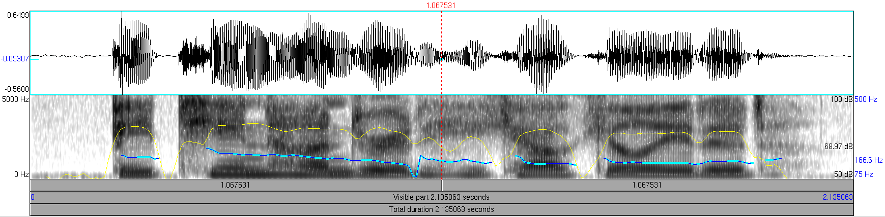
(a) The natural speech of the arctic_a0453 example.

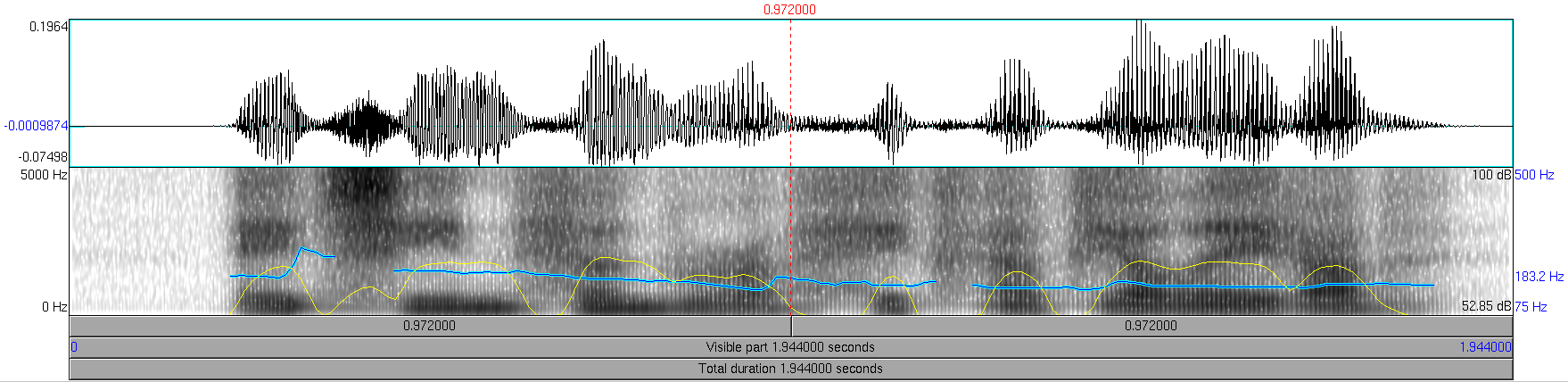
(b) The example generated with the GP features.

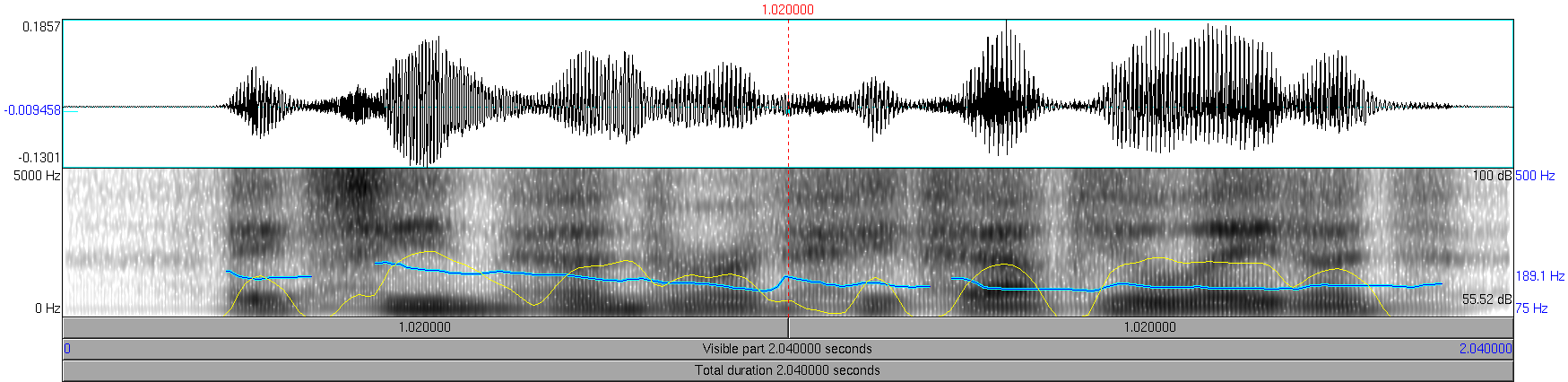
(c) The example generated with the eSPE features

Figure 10: Visualisation of vocoded arctic_a0453 examples: ``Eighteen hundred, he calculated.''. The GP vocoding seems to better synthesise the higher frequencies such as for fricatives, whereas eSPE vocoding seems to synthesise stronger formant frequencies. The recordings are available in B.

Subjective Intelligibility Test

We compared the phonological TTS with a conventional hidden Markov model (HMM) parametric speech synthesizer, trained on the same training set of the audiobook which was used for training the phonological vocoder. For building the HMM models, the HTS V.2.1 toolkit (HTS, 2010) was used. Specifically, the implementation from the EMIME project (Wester et al., 2010) was taken. Five-state, left-to-right, no-skip HSMMs were used. The speech parameters which were used for training the HSMMs were 39 order mel-cepstral coefficients, log-F0 and 21-band aperiodicities, along with their delta and delta-delta features, extracted every 5 ms.

For evaluating the phonological TTS, an intelligibility test was conducted using semantically unpredictable sentences (SUSs). Two sets of sentences were used in this test. Each set contained 14 unique SUSs. The SUSs were taken from SIWIS database Goldman et al. (2016). The length of the sentences varied from 6 to 8 words. Each set consisted of 7 sentences synthesised by the phonological TTS, and another 7 ones synthesised by the reference HTS system.

Twenty native English listeners, experts in the speech processing field, participated in the listening test. The listeners could listen to each synthesized sentence only one or two times, and were asked to transcribe the audio. Eleven and nine listeners respectively participated in the two sets of the listening test. Intelligibility score was calculated by:

$$\mbox{Intelligibility}=\frac{H-I}{N}\mbox{ x 100\%}$$ (5)

where $H$ is the number of correctly transcribed words, $I$ is the number of insertions, and $N$ is the total number of words in the reference transcription.

The average intelligibility score of the phonological TTS was 71% in comparison to the HMM-based TTS where the listeners achieved the intelligibility of 84%. The phonological TTS thus achieved intelligibility of 85% of the state-of-the-art parametric TTS.

Proposed continuous speech synthesis from the phonological speech representation is trained only from speech part of an audio-book without the aligned text transcription, whereas conventional parametric speech synthesis requires aligned phonetic labels for training of the synthesis model. Hence, we consider this approach as unsupervised TTS training.

Cernak et al. (2016) have recently shown that major degradation of speech quality in speech synthesis based on the phonological speech representation comes from the LPC re-synthesis. Therefore, other parametric vocoding is planned in our future work.

6 Conclusions

We have proposed to use speech vocoding as a platform for laboratory phonology. The proposal consists of a cascaded phonological analysis and synthesis. The objective and subjective evaluations supported the hypothesis that the most informative feature set – with the best coverage of the acoustic space (see confusion matrices of context-independent vocoding in Sec. 5.2.1) – achieves the best quality vocoded speech (see context-dependent vocoding in Sec. 5.2.2), where the features are verified in both directions, recognition and synthesis, simultaneously.

We have showed three application examples of our proposed approach. First, we compared three systems of phonological representations and concluded that eSPE achieves slightly better results than the other two. Our results thus support other recent work showing that eSPE is suitable for phonological analysis, for speech recognition and language identification tasks (Yu et al., 2012; Siniscalchi et al., 2012). However, GP – the most compact phonological speech representation, performs in the analysis/synthesis tasks comparably to the systems with higher number of phonological features.

Second, we presented compositional phonological speech modelling, where phonological atoms can generate arbitrary speech sounds. Third, we explored phonological parametric TTS without any front-end, trained from an unlabelled audiobook in an unsupervised manner, and achieving intelligibility of 85% of the state-of-the-art parametric speech synthesis. This seems to be a promising approach for unsupervised and multilingual text-to-speech systems.

In this work we have focused on the segmental evaluation of the phonological systems. In the future, we plan to address this limitation by incorporating supra-segmental features, and using the proposed laboratory phonology platform for further experimentation such as generation of speech stimuli for perception experiments.

We envision that the presented approach paves the way for researchers in both fields to form meaningful hypotheses that are explicitly testable using the concepts developed and exemplified in this paper. Laboratory phonologists might test the compactness, confusability, perceptual viability, and other applied concepts of their theoretical models. This might be done in at least two ways. Firstly, synthesis/recognition tests might follow hand in hand with their analysis of data from human speech production and perception, which would allow for accumulating much needed data on the differences between human and machine performance. Secondly, synthesis/recognition might be used for pre-testing before undergoing experiments and analysis of human data, which is commonly time and effort demanding. This framework can be used in speech processing field as an evaluation platform for improving the performance of current state-of-the-art applications, for example in multi-lingual processing, using the concepts developed for the theoretical phonological models.

7 Acknowledgements

We would like to thank Dr. Phil N.Garner from Idiap Research Institute, for his valuable comments on this paper.

This work has been conducted with the support of the Swiss NSF under grant CRSII2 141903: Spoken Interaction with Interpretation in Switzerland (SIWIS) and grant 2/0197/15 by Scientific Granting Agency in Slovakia.

8 References

Appendix A Mapping of the phonological features to CMUbet

Tables 1, 2 and 3 show the mapping of the phonological features to the used phonemes in this work.

Table 1: GP phonological features and their association to CMUbet phonemes used in this paper.

CMUbet IPA A I U E S h H N a i u silence iy i $-$ $+$ $-$ $-$ $-$ $-$ $-$ $-$ $-$ $+$ $-$ $-$ ih I $-$ $+$ $-$ $+$ $-$ $-$ $-$ $-$ $-$ $-$ $-$ $-$ uw u $-$ $-$ $+$ $-$ $-$ $-$ $-$ $-$ $-$ $-$ $+$ $-$ uh U $-$ $-$ $+$ $+$ $-$ $-$ $-$ $-$ $-$ $-$ $-$ $-$ ey eI $+$ $+$ $-$ $-$ $-$ $-$ $-$ $-$ $-$ $+$ $-$ $-$ ow oU $+$ $-$ $+$ $-$ $-$ $-$ $-$ $-$ $-$ $-$ $+$ $-$ oy oI $+$ $-$ $+$ $-$ $-$ $-$ $-$ $-$ $-$ $+$ $+$ $-$ ao O $+$ $-$ $+$ $+$ $-$ $-$ $-$ $-$ $-$ $-$ $+$ $-$ aa A $+$ $-$ $-$ $-$ $-$ $-$ $-$ $-$ $+$ $-$ $-$ $-$ ae æ $+$ $+$ $-$ $-$ $-$ $-$ $-$ $-$ $+$ $-$ $-$ $-$ ah 2 $+$ $-$ $-$ $+$ $-$ $-$ $-$ $-$ $-$ $-$ $-$ $-$ aw aU $+$ $-$ $+$ $-$ $-$ $-$ $-$ $-$ $-$ $-$ $+$ $-$ ay aI $+$ $+$ $-$ $-$ $-$ $-$ $-$ $-$ $-$ $+$ $-$ $-$ y j $-$ $+$ $-$ $-$ $-$ $-$ $-$ $-$ $-$ $-$ $-$ $-$ w w $-$ $-$ $+$ $-$ $-$ $-$ $-$ $-$ $-$ $-$ $-$ $-$ eh e $+$ $+$ $-$ $+$ $-$ $-$ $-$ $-$ $-$ $+$ $-$ $-$ er 3 $+$ $-$ $-$ $+$ $-$ $-$ $-$ $-$ $-$ $-$ $-$ $-$ r r $+$ $-$ $+$ $+$ $-$ $-$ $-$ $-$ $-$ $-$ $-$ $-$ l l $-$ $-$ $-$ $-$ $+$ $-$ $-$ $-$ $-$ $-$ $-$ $-$ p p $-$ $-$ $+$ $-$ $+$ $+$ $+$ $-$ $-$ $-$ $-$ $-$ b b $-$ $-$ $+$ $-$ $+$ $+$ $-$ $-$ $-$ $-$ $-$ $-$ f f $-$ $-$ $+$ $-$ $-$ $+$ $+$ $-$ $-$ $-$ $-$ $-$ v v $-$ $-$ $+$ $-$ $-$ $+$ $-$ $-$ $-$ $-$ $-$ $-$ m m $-$ $-$ $+$ $-$ $+$ $-$ $-$ $+$ $-$ $-$ $-$ $-$ t t $+$ $-$ $-$ $-$ $+$ $+$ $+$ $-$ $-$ $-$ $-$ $-$ d d $+$ $-$ $-$ $-$ $+$ $+$ $-$ $-$ $-$ $-$ $-$ $-$ th T $+$ $-$ $-$ $-$ $-$ $+$ $+$ $-$ $-$ $-$ $-$ $-$ dh D $+$ $-$ $-$ $-$ $-$ $+$ $-$ $-$ $-$ $-$ $-$ $-$ n n $-$ $-$ $-$ $-$ $+$ $-$ $-$ $+$ $-$ $-$ $-$ $-$ s s $-$ $-$ $-$ $+$ $-$ $+$ $+$ $-$ $-$ $-$ $-$ $-$ z z $-$ $-$ $-$ $+$ $-$ $+$ $-$ $-$ $-$ $-$ $-$ $-$ ch tS $-$ $+$ $-$ $-$ $+$ $-$ $+$ $-$ $-$ $-$ $-$ $-$ jh dZ $-$ $+$ $-$ $-$ $+$ $-$ $-$ $-$ $-$ $-$ $-$ $-$ sh S $-$ $+$ $-$ $-$ $-$ $+$ $+$ $-$ $-$ $-$ $-$ $-$ zh Z $-$ $+$ $-$ $-$ $-$ $+$ $-$ $-$ $-$ $-$ $-$ $-$ k k $-$ $-$ $-$ $+$ $+$ $+$ $+$ $-$ $-$ $-$ $-$ $-$ g g $-$ $-$ $-$ $+$ $+$ $+$ $-$ $-$ $-$ $-$ $-$ $-$ ng N $-$ $-$ $-$ $+$ $+$ $-$ $-$ $+$ $-$ $-$ $-$ $-$ hh h $-$ $-$ $-$ $-$ $-$ $+$ $+$ $-$ $-$ $-$ $-$ $-$

Table 2: SPE phonological features and their association to CMUbet phonemes used in this paper.

CMUbet IPA vocalic consonantal high back low anterior coronal round rising tense voice continuant nasal strident silence iy i $+$ $-$ $+$ $-$ $-$ $-$ $-$ $-$ $-$ $+$ $+$ $+$ $-$ $-$ $-$ ih I $+$ $-$ $+$ $-$ $-$ $-$ $-$ $-$ $-$ $-$ $+$ $+$ $-$ $-$ $-$ uw u $+$ $-$ $+$ $+$ $-$ $-$ $-$ $+$ $-$ $+$ $+$ $+$ $-$ $-$ $-$ uh U $+$ $-$ $+$ $+$ $-$ $-$ $-$ $+$ $-$ $-$ $+$ $+$ $-$ $-$ $-$ ey eI $+$ $-$ $-$ $-$ $-$ $-$ $-$ $-$ $+$ $+$ $+$ $+$ $-$ $-$ $-$ ow oU $+$ $-$ $-$ $+$ $-$ $-$ $-$ $+$ $+$ $+$ $+$ $+$ $-$ $-$ $-$ oy oI $+$ $-$ $-$ $+$ $-$ $-$ $-$ $+$ $+$ $-$ $+$ $+$ $-$ $-$ $-$ ao O $+$ $-$ $-$ $+$ $-$ $-$ $-$ $+$ $-$ $-$ $+$ $+$ $-$ $-$ $-$ aa A $+$ $-$ $-$ $+$ $+$ $-$ $-$ $-$ $-$ $+$ $+$ $+$ $-$ $-$ $-$ ae æ $+$ $-$ $-$ $-$ $+$ $-$ $-$ $-$ $-$ $-$ $+$ $+$ $-$ $-$ $-$ ah 2 $+$ $-$ $-$ $+$ $-$ $-$ $-$ $-$ $-$ $-$ $+$ $+$ $-$ $-$ $-$ aw aU $+$ $-$ $-$ $+$ $+$ $-$ $-$ $-$ $+$ $+$ $+$ $+$ $-$ $-$ $-$ ay aI $+$ $-$ $-$ $-$ $+$ $-$ $-$ $-$ $+$ $+$ $+$ $+$ $-$ $-$ $-$ y j $-$ $-$ $+$ $-$ $-$ $-$ $-$ $-$ $-$ $-$ $+$ $+$ $-$ $-$ $-$ w w $-$ $-$ $+$ $+$ $-$ $-$ $-$ $+$ $-$ $-$ $+$ $+$ $-$ $-$ $-$ eh e $+$ $-$ $-$ $-$ $-$ $-$ $-$ $-$ $-$ $-$ $+$ $+$ $-$ $-$ $-$ er 3 $+$ $-$ $-$ $-$ $-$ $-$ $-$ $-$ $-$ $+$ $+$ $+$ $-$ $-$ $-$ r r $+$ $+$ $-$ $-$ $-$ $-$ $+$ $-$ $-$ $-$ $+$ $+$ $-$ $-$ $-$ l l $+$ $+$ $-$ $-$ $-$ $+$ $+$ $-$ $-$ $-$ $+$ $+$ $-$ $-$ $-$ p p $-$ $+$ $-$ $-$ $-$ $+$ $-$ $-$ $-$ $-$ $-$ $-$ $-$ $-$ $-$ b b $-$ $+$ $-$ $-$ $-$ $+$ $-$ $-$ $-$ $-$ $+$ $-$ $-$ $-$ $-$ f f $-$ $+$ $-$ $-$ $-$ $+$ $-$ $-$ $-$ $-$ $-$ $+$ $-$ $+$ $-$ v v $-$ $+$ $-$ $-$ $-$ $+$ $-$ $-$ $-$ $-$ $+$ $+$ $-$ $+$ $-$ m m $-$ $+$ $-$ $-$ $-$ $+$ $-$ $-$ $-$ $-$ $+$ $-$ $+$ $-$ $-$ t t $-$ $+$ $-$ $-$ $-$ $+$ $+$ $-$ $-$ $-$ $-$ $-$ $-$ $-$ $-$ d d $-$ $+$ $-$ $-$ $-$ $+$ $+$ $-$ $-$ $-$ $+$ $-$ $-$ $-$ $-$ th T $-$ $+$ $-$ $-$ $-$ $+$ $+$ $-$ $-$ $-$ $-$ $+$ $-$ $-$ $-$ dh D $-$ $+$ $-$ $-$ $-$ $+$ $+$ $-$ $-$ $-$ $+$ $+$ $-$ $-$ $-$ n n $-$ $+$ $-$ $-$ $-$ $+$ $+$ $-$ $-$ $-$ $+$ $-$ $+$ $-$ $-$ s s $-$ $+$ $-$ $-$ $-$ $+$ $+$ $-$ $-$ $-$ $-$ $+$ $-$ $+$ $-$ z z $-$ $+$ $-$ $-$ $-$ $+$ $+$ $-$ $-$ $-$ $+$ $+$ $-$ $+$ $-$ ch tS $-$ $+$ $+$ $-$ $-$ $-$ $+$ $-$ $-$ $-$ $-$ $-$ $-$ $+$ $-$ jh dZ $-$ $+$ $+$ $-$ $-$ $-$ $+$ $-$ $-$ $-$ $+$ $-$ $-$ $+$ $-$ sh S $-$ $+$ $+$ $-$ $-$ $-$ $+$ $-$ $-$ $-$ $-$ $+$ $-$ $+$ $-$ zh Z $-$ $+$ $+$ $-$ $-$ $-$ $+$ $-$ $-$ $-$ $+$ $+$ $-$ $+$ $-$ k k $-$ $+$ $+$ $+$ $-$ $-$ $-$ $-$ $-$ $-$ $-$ $-$ $-$ $-$ $-$ g g $-$ $+$ $+$ $+$ $-$ $-$ $-$ $-$ $-$ $-$ $+$ $-$ $-$ $-$ $-$ ng N $-$ $+$ $+$ $+$ $-$ $-$ $-$ $-$ $-$ $-$ $+$ $-$ $+$ $-$ $-$ hh h $-$ $-$ $-$ $-$ $+$ $-$ $-$ $-$ $-$ $-$ $-$ $+$ $-$ $-$ $-$

Table 3: eSPE phonological features and their association to CMUbet phonemes used in this paper.

CMUbet IPA vowel fricative nasal stop approxim. coronal high dental glottal labial low mid retroflex velar anterior back continuant round tense voiced silence iy i $+$ $-$ $-$ $-$ $-$ $-$ $+$ $-$ $-$ $-$ $-$ $-$ $-$ $-$ $-$ $-$ $+$ $-$ $+$ $+$ $-$ ih I $+$ $-$ $-$ $-$ $-$ $-$ $+$ $-$ $-$ $-$ $-$ $-$ $-$ $-$ $-$ $-$ $+$ $-$ $-$ $+$ $-$ uw u $+$ $-$ $-$ $-$ $-$ $-$ $+$ $-$ $-$ $-$ $-$ $-$ $-$ $-$ $-$ $+$ $+$ $+$ $+$ $+$ $-$ uh U $+$ $-$ $-$ $-$ $-$ $-$ $+$ $-$ $-$ $-$ $-$ $-$ $-$ $-$ $-$ $+$ $+$ $+$ $-$ $+$ $-$ ey eI $+$ $-$ $-$ $-$ $-$ $-$ $-$ $-$ $-$ $-$ $-$ $+$ $-$ $-$ $-$ $-$ $+$ $-$ $+$ $+$ $-$ ow oU $+$ $-$ $-$ $-$ $-$ $-$ $+$ $-$ $-$ $-$ $-$ $+$ $-$ $-$ $-$ $+$ $+$ $+$ $+$ $+$ $-$ oy oI $+$ $-$ $-$ $-$ $-$ $-$ $-$ $-$ $-$ $-$ $-$ $-$ $-$ $-$ $-$ $+$ $+$ $+$ $-$ $+$ $-$ ao O $+$ $-$ $-$ $-$ $-$ $-$ $-$ $-$ $-$ $-$ $-$ $-$ $-$ $-$ $-$ $+$ $+$ $+$ $+$ $+$ $-$ aa A $+$ $-$ $-$ $-$ $-$ $-$ $-$ $-$ $-$ $-$ $+$ $-$ $-$ $-$ $-$ $+$ $+$ $-$ $+$ $+$ $-$ ae æ $+$ $-$ $-$ $-$ $-$ $-$ $-$ $-$ $-$ $-$ $+$ $-$ $-$ $-$ $-$ $-$ $+$ $-$ $+$ $+$ $-$ ah 2 $+$ $-$ $-$ $-$ $-$ $-$ $-$ $-$ $-$ $-$ $-$ $+$ $-$ $-$ $-$ $+$ $+$ $-$ $-$ $+$ $-$ aw aU $+$ $-$ $-$ $-$ $-$ $-$ $-$ $-$ $-$ $-$ $+$ $-$ $-$ $-$ $-$ $+$ $+$ $+$ $+$ $+$ $-$ ay aI $+$ $-$ $-$ $-$ $-$ $-$ $-$ $-$ $-$ $-$ $+$ $-$ $-$ $-$ $-$ $+$ $+$ $-$ $+$ $+$ $-$ y j $-$ $-$ $-$ $-$ $+$ $-$ $+$ $-$ $-$ $-$ $-$ $-$ $-$ $-$ $-$ $-$ $+$ $+$ $-$ $+$ $-$ w w $-$ $-$ $-$ $-$ $+$ $-$ $-$ $-$ $-$ $+$ $-$ $-$ $-$ $-$ $+$ $-$ $+$ $+$ $-$ $+$ $-$ eh e $+$ $-$ $-$ $-$ $-$ $-$ $-$ $-$ $-$ $-$ $-$ $+$ $-$ $-$ $-$ $-$ $+$ $-$ $-$ $+$ $-$ er 3 $+$ $-$ $-$ $-$ $-$ $-$ $-$ $-$ $-$ $-$ $-$ $-$ $+$ $-$ $-$ $-$ $+$ $-$ $-$ $+$ $-$ r r $-$ $-$ $-$ $-$ $+$ $-$ $-$ $-$ $-$ $-$ $-$ $-$ $+$ $-$ $-$ $-$ $+$ $+$ $-$ $+$ $-$ l l $-$ $-$ $-$ $-$ $+$ $+$ $-$ $-$ $-$ $-$ $-$ $-$ $-$ $-$ $-$ $-$ $+$ $-$ $-$ $+$ $-$ p p $-$ $-$ $-$ $+$ $-$ $-$ $-$ $-$ $-$ $+$ $-$ $-$ $-$ $-$ $+$ $-$ $-$ $-$ $+$ $-$ $-$ b b $-$ $-$ $-$ $+$ $-$ $-$ $-$ $-$ $-$ $+$ $-$ $-$ $-$ $-$ $+$ $-$ $-$ $-$ $-$ $+$ $-$ f f $-$ $+$ $-$ $-$ $-$ $-$ $-$ $-$ $-$ $+$ $-$ $-$ $-$ $-$ $+$ $-$ $+$ $-$ $+$ $-$ $-$ v v $-$ $+$ $-$ $-$ $-$ $-$ $-$ $-$ $-$ $+$ $-$ $-$ $-$ $-$ $+$ $-$ $+$ $+$ $-$ $+$ $-$ m m $-$ $-$ $+$ $-$ $-$ $-$ $-$ $-$ $-$ $+$ $-$ $-$ $-$ $-$ $+$ $-$ $-$ $-$ $-$ $+$ $-$ t t $-$ $-$ $-$ $+$ $-$ $+$ $-$ $-$ $-$ $-$ $-$ $-$ $-$ $-$ $+$ $-$ $-$ $-$ $+$ $-$ $-$ d d $-$ $-$ $-$ $+$ $-$ $+$ $-$ $-$ $-$ $-$ $-$ $-$ $-$ $-$ $+$ $-$ $-$ $-$ $-$ $+$ $-$ th T $-$ $+$ $-$ $-$ $-$ $-$ $-$ $+$ $-$ $-$ $-$ $-$ $-$ $-$ $+$ $-$ $+$ $-$ $+$ $-$ $-$ dh D $-$ $+$ $-$ $-$ $-$ $-$ $-$ $+$ $-$ $-$ $-$ $-$ $-$ $-$ $+$ $-$ $+$ $-$ $-$ $+$ $-$ n n $-$ $-$ $+$ $-$ $-$ $+$ $-$ $-$ $-$ $-$ $-$ $-$ $-$ $-$ $+$ $-$ $-$ $-$ $-$ $+$ $-$ s s $-$ $+$ $-$ $-$ $-$ $+$ $-$ $-$ $-$ $-$ $-$ $-$ $-$ $-$ $+$ $-$ $+$ $-$ $+$ $-$ $-$ z z $-$ $+$ $-$ $-$ $-$ $+$ $-$ $-$ $-$ $-$ $-$ $-$ $-$ $-$ $+$ $-$ $+$ $-$ $-$ $+$ $-$ ch tS $-$ $+$ $-$ $-$ $-$ $-$ $+$ $-$ $-$ $-$ $-$ $-$ $-$ $-$ $-$ $-$ $-$ $-$ $+$ $-$ $-$ jh dZ $-$ $+$ $-$ $-$ $-$ $-$ $+$ $-$ $-$ $-$ $-$ $-$ $-$ $-$ $-$ $-$ $-$ $-$ $-$ $+$ $-$ sh S $-$ $+$ $-$ $-$ $-$ $-$ $+$ $-$ $-$ $-$ $-$ $-$ $-$ $-$ $-$ $-$ $+$ $-$ $+$ $-$ $-$ zh Z $-$ $+$ $-$ $-$ $-$ $-$ $-$ $-$ $-$ $-$ $-$ $-$ $-$ $-$ $-$ $-$ $-$ $-$ $-$ $-$ $-$ k k $-$ $-$ $-$ $+$ $-$ $-$ $+$ $-$ $-$ $-$ $-$ $-$ $-$ $+$ $-$ $+$ $-$ $-$ $+$ $-$ $-$ g g $-$ $-$ $-$ $+$ $-$ $-$ $+$ $-$ $-$ $-$ $-$ $-$ $-$ $+$ $-$ $+$ $-$ $-$ $-$ $+$ $-$ ng N $-$ $-$ $+$ $-$ $-$ $-$ $+$ $-$ $-$ $-$ $-$ $-$ $-$ $+$ $-$ $-$ $-$ $-$ $-$ $+$ $-$ hh h $-$ $-$ $-$ $-$ $-$ $-$ $-$ $-$ $+$ $-$ $-$ $-$ $-$ $-$ $-$ $-$ $-$ $-$ $-$ $-$ $-$

Appendix B Demonstrating speech synthesis samples

Tables 1 and 2 contain recordings demonstrating GP phonological atoms and their composition, respectively, and Table 3 contains recordings demonstrating phonological speech synthesis.

Table 1: Recordings demonstrating individual phonological atoms. The $z_{n}^{k}$ patterns were repeated to get phonological atoms $\mathbf{a}^{k}$ of two seconds long.

Phonolog. atom Recording Offline link $\mathbf{a}^{A}$ (wav) www.idiap.ch/paper/3120/A.wav $\mathbf{a}^{a}$ (wav) %**** appendixs.tex Line 25 ****www.idiap.ch/paper/3120/a.wav $\mathbf{a}^{I}$ (wav) www.idiap.ch/paper/3120/I.wav $\mathbf{a}^{i}$ (wav) www.idiap.ch/paper/3120/i.wav $\mathbf{a}^{U}$ (wav) www.idiap.ch/paper/3120/U.wav $\mathbf{a}^{u}$ (wav) www.idiap.ch/paper/3120/u.wav $\mathbf{a}^{E}$ (wav) %**** appendixs.tex Line 50 ****www.idiap.ch/paper/3120/E.wav $\mathbf{a}^{H}$ (wav) www.idiap.ch/paper/3120/H.wav $\mathbf{a}^{h}$ (wav) www.idiap.ch/paper/3120/h.wav $\mathbf{a}^{S}$ (wav) www.idiap.ch/paper/3120/S.wav $\mathbf{a}^{N}$ (wav) www.idiap.ch/paper/3120/N.wav

Table 2: Recordings demonstrating composition of GP phonological atoms, resulting into the synthesis of new sounds.

Rule IPA Composition Offline link [A, I, U, E] œ (wav) www.idiap.ch/paper/3120/oe.wav [I, U, E] y (wav) www.idiap.ch/paper/3120/u.wav

Table 3: Recordings demonstrating phonological speech synthesis.

Sentence Scheme Recording Offline link a0453 GP (wav) www.idiap.ch/paper/3120/a0453-GP.wav SPE (wav) www.idiap.ch/paper/3120/a0453-SPE.wav eSPE (wav) www.idiap.ch/paper/3120/a0453-eSPE.wav a0457 GP (wav) www.idiap.ch/paper/3120/a0457-GP.wav SPE (wav) www.idiap.ch/paper/3120/a0457-SPE.wav eSPE (wav) www.idiap.ch/paper/3120/a047-eSPE.wav a0460 GP (wav) www.idiap.ch/paper/3120/a0460-GP.wav SPE (wav) www.idiap.ch/paper/3120/a0460-SPE.wav eSPE (wav) www.idiap.ch/paper/3120/a0460-eSPE.wav

References

- Bever and Poeppel (2010) Bever, T. G., Poeppel, D., 2010. Analysis by Synthesis: A (Re-)Emerging Program of Research for Language and Vision. Biolinguistics 4 (2-3), 174–200.
- Cernak et al. (2016) Cernak, M., Lazaridis, A., Asaei, A., Garner, P. N., August 2016. Composition of Deep and Spiking Neural Networks for Very Low Bit Rate Speech Coding. IEEE Trans. on Audio, Speech, and Language Processing.
-