Large deviations for the height in 1D Kardar-Parisi-Zhang growth at late times

Abstract

We study the atypically large deviations of the height $H\sim{{\cal O}}(t)$ at the origin at late times in $1+1$-dimensional growth models belonging to the Kardar-Parisi-Zhang (KPZ) universality class. We present exact results for the rate functions for the discrete single step growth model, as well as for the continuum KPZ equation in a droplet geometry. Based on our exact calculation of the rate functions we argue that models in the KPZ class undergo a third order phase transition from a strong coupling to a weak coupling phase, at late times.

The celebrated Tracy-Widom (TW) distribution was discovered originally in random matrix theory (RMT) TW94 ; TW96 . In RMT, it describes the probability distribution of the typical fluctuations of the largest eigenvalue of a Gaussian random matrix. Since then, this distribution has emerged in a variety of problems TW_review ; Wolchover (unrelated a priori to RMT), ranging from random permutations baik all the way up to the Yang-Mills gauge field theory FMS11 . Why is TW distribution so ubiquitous? It was recently shown that in several systems where TW distribution occurs there is usually an underlying third order phase transition between a strong and a weak coupling phase rmt_review . In these systems the TW distribution appears as a finite-size crossover function connecting the free-energies of the two phases across the third order critical point rmt_review . In the strong coupling phase, the degrees of freedom of the system act collectively while the weak coupling phase is described by a single dominant degree of freedom. In the context of RMT, this third-order phase transition shows up in the distribution of the top eigenvalue $\lambda_{\max}$ of a $N\times N$ matrix belonging to the classical Gaussian ensembles rmt_review . The central part of the distribution, corresponding to the typical fluctuations of $\lambda_{\max}$, is described by the TW distribution, while the atypically large fluctuations to the left (right) correspond to the strong (respectively weak) coupling phases.

For a wide class of 1+1-dimensional interface growth models belonging to the Kardar-Parisi-Zhang (KPZ) universality class KPZ , it is well known that the typical height fluctuations grow at late times as $\sim t^{1/3}$ directedpoly . Moreover the probability distribution function (PDF) of these typical fluctuations are given by the TW distribution johansson ; spohn2000 ; TW2001 ; Majumdar2004 ; MN2005 ; SS10 ; CLR10 ; DOT10 ; ACQ11 ; reviewCorwin . This TW distribution has also been verified experimentally in liquid crystal and paper burning systems takeuchi ; myllys ; HH-TakeuchiReview . The appearance of the TW distribution in these growth models then raises a natural question: is there a third order phase transition between a strong and a weak coupling phase in such growth models? If so, how can one describe these two phases? In this Letter, we show that there is indeed a third order phase transition in these growth models by studying the probability distribution $P(H,t)$ of the height $H$ at the origin (suitably centered) at late times $t\gg 1$. Specifically, we find that $P(H,t)$, for $t\gg 1$, has three different behaviors

$$P(H,t)\sim\begin{cases}&e^{-t^{2}\,\Phi_{-}(H/t)}\quad,\quad H\sim{\cal O}(t)<0\;\quad{\rm I}\\ &\\ &\dfrac{1}{t^{1/3}}f\left[\dfrac{H}{t^{1/3}}\right]\;,\;\hskip 8.5359ptH\sim{\cal O}(t^{1/3})\quad{\rm II}\\ &\\ &e^{-t\,\Phi_{+}(H/t)}\quad,\quad H\sim{\cal O}(t)>0\quad{\rm III}\;.\end{cases}$$ (1)

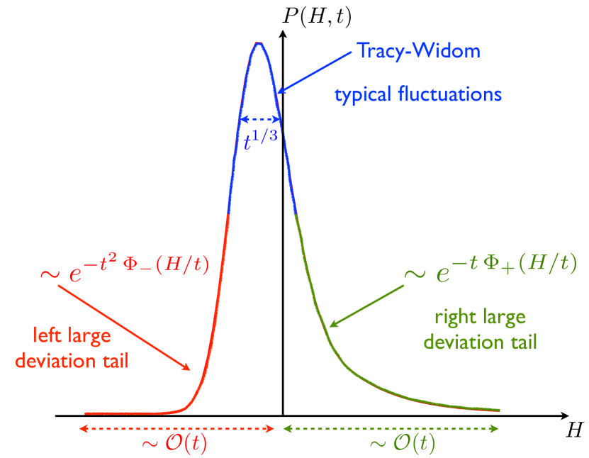
Figure 1: A schematic picture of the height distribution at the origin. The typical fluctuations $H\sim{\cal O}(t^{1/3})$ around the mean are distributed according to the Tracy-Widom GUE law (blue line). The atypical large fluctuations to the left (red line) and to the right (green line) are described respectively by the left and right large deviation functions in Eq. (1).

The regime II is well known and it describes the typical height fluctuations ($H\sim{\cal O}(t^{1/3})$) and the scaling function $f(s)$ is given by the TW distribution. The scaling function depends on the initial conditions: for the flat geometry it corresponds to $f_{1}(s)$ (i.e., TW for the Gaussian Orthogonal Ensemble, GOE), while for the curved (or droplet) geometry, it corresponds to $f_{2}(s)$ (i.e., TW for the Gaussian Unitary Ensemble, GUE). These distributions have asymmetric non-Gaussian tails:

$$f_{\beta}(s)\sim\begin{cases}&e^{-\frac{\beta}{24}|s|^{3}}\;,\;s\to-\infty\\ &e^{-\frac{2\beta}{3}s^{3/2}}\;,\;s\to+\infty\;,\end{cases}$$ (2)

where $\beta=1$ and $2$ correspond respectively to GOE and GUE.

The new results in this Letter concern the atypical large height fluctuations in regime I and III in Eq. (1). The regime I corresponds to the large negative fluctuations ($H\sim{\cal O}(t)<0$) and is characterized by the left large deviation function $\Phi_{-}(z)$. Similarly, the regime III describes the large positive fluctuations ($H\sim{\cal O}(t)>0$) and is characterized by the right large deviation function $\Phi_{+}(z)$. These two rate functions $\Phi_{\pm}(z)$ are the characteristics of the two phases: $\Phi_{-}(z)$ corresponds to the strong coupling phase, while $\Phi_{+}(z)$ describes the weak coupling phase (as explained later). Note that on the scale $H\sim{\cal O}(t)$, the central part of width ${\cal O}(t^{1/3})$ is effectively reduced to a point $z=0$ as $t\to\infty$. Indeed, it follows from Eq. (1) that

$$\lim_{t\to\infty}-\frac{1}{t^{2}}\ln P(H=z\,t,t)=\begin{cases}&\Phi_{-}(z)\;,\;z\leq 0\\ &0\;,\;z\geq 0\;.\end{cases}$$ (3)

Thus as $t\to\infty$, $z=0$ becomes a critical point and $\Phi_{-}(z)$ can be interpreted as the “free energy” of the strong coupling phase. We further show that it vanishes universally, $\Phi_{-}(z)\propto|z|^{3}$, as $z\to 0^{-}$, thus indicating a third order phase transition. Therefore in order to probe this third order transition it is important to compute the large deviation functions. In this Letter, we compute $\Phi_{\pm}(z)$ explicitly for the droplet geometry in (i) a discrete single step growth model belonging to the KPZ class and (ii) the continuum KPZ equation. In general, $\Phi_{\pm}(z)$ are non-universal and depend on the model. However, their small arguments behaviors are universal: $\Phi_{-}(z)\propto|z|^{3}$ as $z\to 0^{-}$ and $\Phi_{+}(z)\propto z^{3/2}$ as $z\to 0^{+}$. Indeed, as the critical point $z=0$ is approached from either side, the large deviation behaviors smoothly match with the asymptotic tails of the TW distribution (2).

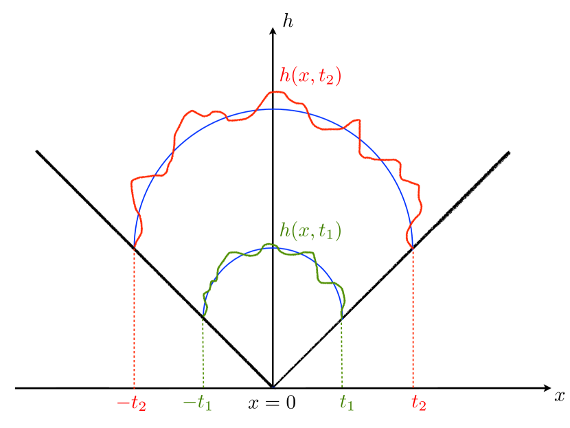
Figure 2: The height $h(x,t)$ evolving on a substrate $-t\leq x\leq t$. The light cone (black lines) describes the evolution of the substrate. The solid line (in blue) represents the average height at two different times, $\langle h(x,t)\rangle=v(x/t)\,t$ with $v(z)=1+\sqrt{1-z^{2}}$ having a semi-circular shape.

We start by analyzing a directed polymer model belonging to the KPZ universality class studied by Johansson johansson . This model can be translated to a discrete space-time $(x,t)$ growth model in a “droplet” geometry. The growth takes place on the substrate $-t\leq x\leq t$ (see Fig. 2), starting from the seed at the origin $x=0$ at $t=0$. The interface height $h(x,t)$, at site $x$ and at time $t$, evolves in the bulk $-t<x<t$ as footnote_edge

$$h(x,t)={\rm max}[h(x-1,t-1),h(x+1,t-1)]+\eta(x,t)\,$$ (4)

where $\eta(x,t)\geq 0$’s are independent and identically distributed (i.i.d.) nonnegative random variables each drawn from an exponential distribution: $p(\eta)=e^{-\eta}$ for $\eta\geq 0$. Johansson showed that at late times, the average height $\langle h(x,t)\rangle=v(x/t)\,t$ with $v(z)=1+\sqrt{1-z^{2}}$ exhibiting a semi-circular droplet shape (see Fig. 2). Moreover the height at the origin at late times behaves as $h(0,t)\simeq 2\,t+2\,t^{1/3}\chi_{2}$, where $\chi_{2}$ is a $t$-independent random variable distributed via the TW distribution for the GUE, $f_{2}(s)$ johansson . By exploiting an exact mapping to the largest eigenvalue of complex Wishart matrices johansson , and using the results for the large deviations of the latter VMB ; MV , we establish the result in Eq. (1) (with $H=\frac{h(0,t)}{2}-t$). In regime I, we get supp_mat :

$$\Phi_{-}(z)=\frac{1}{8}\left(2z-z^{2}-2\,\ln{(1+z)}\right)\;,\;-1<z\leq 0\;,$$ (5)

where $z>-1$ since the height $h(0,t)>0$. As $z\to 0^{-}$, one gets $\Phi_{-}(z)\sim|z|^{3}/12$ as announced in the introduction. In regime III, we find

$$\Phi_{+}(z)=2\sqrt{z(z+1)}+\ln{\left(2z+1-2\sqrt{z(z+1)}\right)}\;,\;z\geq 0\;,$$ (6)

which behaves as $\Phi_{+}(z)\sim(4/3)z^{3/2}$ as $z\to 0^{+}$. Note that in regime II, if we make $H\sim{\cal O}(t)$ and use the asymptotic behaviors of TW distribution in Eq. (2) with $\beta=2$, it can be checked that it matches smoothly with the large deviation regimes on both sides. Interestingly, in this height model (4) there is a clear physical explanation as to why the left tail [regime I in (1)] scales like $\sim e^{-t^{2}}$ while the right tail [regime III in (1)] behaves like $\sim e^{-t}$. Indeed, in order to realize a configuration of $H$ much smaller than its typical value (regime I), the noise variables $\eta(x,t)$ at all the sites within the $1+1$-dimensional wedge (cf Fig. 2) should be small. Indeed, if any of the $\eta(x,t)$ within this wedge is big, the dynamics in Eq. (4) would force the neighboring sites at the next time step to be big. The probability of this event, where collectively all the noise variables $\eta(x,t)$ inside the wedge ($|x|<t$), of area $\propto t^{2}$, are all small is proportional to $e^{-t^{2}}$ (the noise variables being i.i.d.). In contrast, a configuration where $H$ is much bigger than its typical value (regime III) can be realized by adding large positive noise variables at the origin $\eta(x=0,\tau)$ at all times $\tau$ between $0$ and $t$. The probability of this event is simply $\propto e^{-t}$ as the noises at different times are i.i.d. Hence this event is not a collective one, unlike the left large deviation. Thus, the left large deviation [regime I in Eq. (1)] is the analogue of the ‘strong coupling phase’ and the right large deviation [regime II in Eq. (1)] corresponds to the ‘weak coupling’ phase. The transition between the two phases is a third order phase transition, as $\Phi_{-}(z)\propto|z|^{3}$ as $z\to 0^{-}$, as mentioned above. This picture is very similar to other third order phase transitions observed before in RMT and reviewed recently in Ref. rmt_review .

While the right tail rate function $\Phi_{+}(z)$ has been studied numerically Monthus and, more recently, analytically LogGamma in discrete growth models, the left tail $\Phi_{-}(z)$ is much harder to compute, and there are very few exact results, an exception being the longest increasing subsequence in random permutations (for both tails) Zeitouni . We now show that these rate functions can also be calculated for the continuum KPZ equation itself, where the height field $h(x,t)$ evolves as KPZ

$$\partial_{t}h=\nu\,\partial_{x}^{2}h+\frac{\lambda_{0}}{2}\,(\partial_{x}h)^{2}+\sqrt{D}\,\xi(x,t)\;,$$ (7)

where $\nu>0$ is the coefficient of diffusive relaxation, $\lambda_{0}>0$ is the strength of the non-linearity and $\xi(x,t)$ is a Gaussian white noise with zero mean and $\langle\xi(x,t)\xi(x^{\prime},t^{\prime})\rangle=\delta(x-x^{\prime})\delta(t-t^{\prime})$. We use everywhere the natural units of space $x^{*}=(2\nu)^{3}/(D\lambda_{0}^{2})$, time $t^{*}=2(2\nu)^{5}/(D^{2}\lambda_{0}^{4})$ and height $h^{*}=\frac{2\nu}{\lambda_{0}}$.

Here for definiteness we focus on the narrow wedge initial condition, $h(x,0)=-|x|/\delta$, with $\delta\ll 1$, which gives rise to a curved (or droplet) mean profile as time evolves  SS10 ; CLR10 ; DOT10 ; ACQ11 ; reviewCorwin . We focus on the shifted height at the origin at $x=0$, $H(t)=h(0,t)+\frac{t}{12}$, which fluctuates typically on a scale $t^{1/3}$ around its mean at large time, as described by the regime II in Eq. (1) with $f(s)=f_{2}(s)$, the TW distribution for the GUE.

We show below that for the continuum KPZ equation, in a droplet geometry, the generic result in Eq. (1) holds in regime I and III as well. Interestingly the rate functions turn out to be rather simple in this case

$$\Phi_{-}(z)=\frac{1}{12}|z|^{3}\quad,\quad z\leq 0$$ (8)

$$\Phi_{+}(z)=\dfrac{4}{3}z^{3/2}\quad,\quad z\geq 0\;.$$ (9)

Thus the continuum KPZ equation also exhibits a third order phase transition at the critical point $z=0$.

To derive the rate functions for the continuum KPZ case, we start from an exact formula SS10 ; CLR10 ; DOT10 ; ACQ11 , valid at all times $t$ in the droplet geometry. It relates the following generating function to a Fredholm determinant (FD)

$$g_{t}(s):=\langle\exp(-e^{H(t)-t^{1/3}s})\rangle\;=\det(I-P_{s}K_{t}P_{s})$$ (10)

where the finite time kernel is

$$K_{t}(r,r^{\prime})=\int_{-\infty}^{\infty}du\frac{{\rm Ai}(r+u){\rm Ai}(r^{\prime}+u)}{1+e^{-t^{1/3}u}}\;$$ (11)

and $P_{s}$ is the projector on the interval $[s,+\infty)$ footnote_Fredholm . In Eq. (11), ${\rm Ai}(x)$ denotes the Airy function.

Let us recall that to obtain the typical fluctuations regime (II) in formula (1), where $H(t)\sim t^{1/3}$, one needs to take the limit $t\to+\infty$ at fixed $s$ in (10). In that limit $K_{t}(r,r^{\prime})$ converges to the standard Airy kernel, $K_{\rm Ai}(r,r^{\prime})=\int_{0}^{\infty}du\,{\rm Ai}(r+u){\rm Ai}(r^{\prime}+u)$ and the right hand side (r.h.s.) converges to the GUE-TW distribution. The left hand side (l.h.s.) of (10) converges to $\langle\theta(s-t^{-1/3}H(y))\rangle$ (where $\theta(x)$ is the Heaviside step function), and one obtains

$$\lim_{t\to+\infty}\,{\rm Prob.}(\chi_{t}<s)=\det(I-P_{s}K_{Ai}P_{s})=F_{2}(s)$$ (12)

where $F_{2}(s)=\int_{-\infty}^{s}f_{2}(s^{\prime})ds^{\prime}$ is the cumulative distribution function (CDF) of the GUE-TW distribution. To compute the rate functions $\Phi_{\pm}(z)$ we now consider the formula (10) in the limit when $s$ and $t$ are both large, keeping the ratio $y=s/t^{2/3}$ fixed.

Right tail. We start with the right large deviation function, therefore we consider formula (10) in the regime of large $s>0$. Consider first the l.h.s. of Eq. (10). It is convenient to introduce a random variable $\gamma$ (independent of $H$) distributed via the Gumbel distribution, of CDF given by

$$\langle\theta(b-\gamma)\rangle_{\gamma}=e^{-e^{-b}}\;.$$ (13)

Substituting $b=st^{1/3}-H$ in (13) allows us to rewrite the l.h.s of (10) as

$$1-\langle\exp(-e^{H(t)-t^{1/3}s})\rangle=\langle{\rm Prob}(H>st^{1/3}-\gamma)\rangle_{\gamma}\;.$$ (14)

Now consider the r.h.s of Eq. (10) for $s\gg 1$. Expanding the FD in powers of $K_{t}$ and keeping only the first two terms one obtains

$$\det(I-P_{s}K_{t}P_{s})\simeq 1-\int_{s}^{+\infty}drK_{t}(r,r)\;.$$ (15)

Equating Eq. (14) and (15) and taking a derivative with respect to $s$ gives

$$t^{1/3}\langle P(H=st^{1/3}-\gamma,t)\rangle_{\gamma}=K_{t}(s,s)$$ (16)

a relation exact for all $t$.

We first study the asymptotics of $K_{t}(s,s)$ for large $s\sim t^{2/3}$. Performing a change of variable $u=-t^{2/3}v$, (11) becomes

$$K_{t}(yt^{2/3},yt^{2/3})=t^{2/3}\int_{-\infty}^{+\infty}dv\frac{{\rm Ai}^{2}(t^{2/3}(y-v))}{1+e^{tv}}$$ (17)

with $y={\cal O}(1)$. This integral can be analyzed for large $t$ supp_mat and we obtain footnote2

$$K_{t}(yt^{2/3},yt^{2/3})\sim e^{-tI(y)}\;,\;I(y)=\begin{cases}\frac{4}{3}y^{3/2}\,,\,0<y<\frac{1}{4}\\ y-\frac{1}{12}\,,\,y>\frac{1}{4}\;,\end{cases}$$ (18)

where the pre-exponential factors are given in supp_mat . Having obtained the r.h.s of (16) we now consider its l.h.s. We anticipate (and verify a posteriori) that in this right tail the PDF has the form (setting $z=H/t$)

$$\ln P(H,t)=-t\frac{4}{3}z^{3/2}-a\ln t-\chi_{\rm droplet}(z)+o(1)$$ (19)

where the constant $a$ and the function $\chi_{\rm droplet}(z)$ are yet to be determined. Inserting this form on the l.h.s. of Eq. (16), analyzing the resulting integral supp_mat and comparing it to the r.h.s. in (18), we find that indeed the ansatz in (19) is correct with $a=1$ and an explicit form for $\chi_{\rm droplet}(z)$ given in Eq. (80) of the Supp. Mat. supp_mat . Finally, keeping only the leading behavior of (19) gives us the exact right rate function

$$\Phi_{+}(z)=\frac{4}{3}z^{3/2}\quad,\quad z\geq 0\;,$$ (20)

as announced in Eq. (9). For the pre-exponential factor in the flat case we find $a=1/2$ and $\chi_{\rm flat}(z)$ given in Eq. (87) of the Supp. Mat. supp_mat .

This result is also consistent with the known exact large time behavior of the moments, $\overline{e^{nH}}\sim_{t\to+\infty}e^{\frac{1}{12}n^{3}t}$, calculated using the Bethe ansatz kardareplica . Indeed a saddle point calculation using $P(H,t)\sim e^{-\frac{4}{3}(\frac{H}{t^{1/3}})^{3/2}}$ reads

$$\int dH~{}e^{nH-\frac{4}{3}(\frac{H}{t^{1/3}})^{3/2}}\sim e^{\frac{1}{12}n^{3}t}$$ (21)

where the saddle point, at $H_{n}=n^{2}t/4$ for fixed integer $n$, is precisely in the right large deviation regime. Note that the dependence on the initial condition appears only in the (subdominant) pre-exponential factor of the moments, as discussed in supp_mat where we establish that $\Phi_{+}(z)=\frac{4}{3}z^{3/2}$ both for droplet and flat initial conditions.

Left tail. We now focus on the left tail where we set $H/t\sim{\cal O}(1)<0$. In this case, one can show supp_mat that the l.h.s. of (10) scales as $\sim e^{-t^{2}\Phi_{-}(y=s/t^{2/3})}$ for $y={\cal O}(1)$. The r.h.s of (10), $Q_{t}(s):=\det(I-P_{s}K_{t}P_{s})$, is not easy to analyze in the regime of large negative $s$. Fortunately in Ref. ACQ11 the authors proved an exact differential equation satisfied by $Q_{t}(s)$:

$$\partial_{s}^{2}\ln Q_{t}(s)=-\int_{-\infty}^{+\infty}dv\sigma^{\prime}_{t}(v)[q_{t}(s,v)]^{2}$$ (22)

where

$$\sigma_{t}(v)=\frac{1}{1+e^{-t^{1/3}v}}$$ (23)

and $\sigma_{t}^{\prime}(v)=\partial_{v}\sigma_{t}(v)$. The function $q_{t}(s,v)$ satisfies a non-linear integro-differential equation in the $s$ variable

$$\partial_{s}^{2}q_{t}(s,v)=(s+v+2\int_{-\infty}^{+\infty}dw\sigma^{\prime}_{t}(w)[q_{t}(s,w)]^{2})q_{t}(s,v)$$ (24)

with the boundary condition $q_{t}(s,v)\simeq_{s\to+\infty}{\rm Ai}(s+v)$. In the long limit $t\to+\infty$, $\sigma_{t}^{\prime}(v)\to\delta(v)$ and hence $q_{t}(s,0)$ satisfies the standard Painlevé II equation TW94 .

For large but finite $t$, we substitute the anticipated scaling form $Q_{t}(s)\sim e^{-t^{2}\Phi_{-}(y=s/t^{2/3})}$ in (22). The consistency then suggests that $q_{t}(s,v)$ takes the scaling form

$$q_{t}(s,v)\simeq t^{1/3}\tilde{q}(s/t^{2/3},vt^{1/3})\,,\;{\rm for}\;t\;\to\infty\;,$$ (25)

and the scaling function $\tilde{q}(y,v)$ satisfies

$$\int_{-\infty}^{+\infty}dv\frac{\tilde{q}(y,v)^{2}e^{-v}}{(1+e^{-v})^{2}}=\Phi^{\prime\prime}_{-}(y).$$ (26)

Substituting further the scaling form (25) in the differential equation (24) we obtain as $t\to\infty$

$$y+2\int_{-\infty}^{+\infty}dv\frac{\tilde{q}(y,v)^{2}e^{-v}}{(1+e^{-v})^{2}}=0\;.$$ (27)

Comparing with (26) immediately gives for all $z\leq 0$, $\Phi^{\prime\prime}_{-}(z)=-\frac{z}{2}$. Solving with the boundary condition $\Phi_{-}(z)\simeq_{z\to 0}|z|^{3}/12$, coming from matching with the left tail of the TW GUE distribution as $z\to 0^{-}$, implies

$$\Phi_{-}(z)=\frac{1}{12}|z|^{3}\quad,\quad z\leq 0\;,$$ (28)

as announced in Eq. (8).

In summary, our results on large deviations for the height at late times for growth models in the KPZ class suggest a third order phase transition between a strong and a weak coupling phase. Generically the associated rate functions are non-universal but their small argument behavior are universal, as they match the TW tails. In the case of the continuum KPZ equation these functions are simple, Eqs. (8, 9), showing that the TW universality extends all the way to the large deviation regime. A natural question is how this late time behavior is approached as time increases. Weak noise expansion and instanton calculations in the tails (for the flat geometry) indicate a different behavior $P(H,t)\sim e^{-|H|^{5/2}/t^{1/2}}$ in the left tail in the early time regime $t\ll 1$ Baruch ; Korshunov . In fact we have computed exactly the short time height distribution in the droplet geometry which exhibits a similar $|H|^{5/2}$ left tail behavior us , manifestly different from the late time behavior $|H|^{3}$ obtained here at late times. In contrast, the right tail $H^{3/2}$ is already attained at early time.

We thank D. Dean, B. Meerson, J. Quastel, H. Spohn and K. Takeuchi for useful discussions. We acknowledge support from PSL grant ANR-10-IDEX-0001-02-PSL (PLD). We thank the hospitality of KITP, under Grant No. NSF PHY11-25915.

.

SUPPLEMENTARY MATERIAL

I Johansson model

Johansson’s directed polymer model in $2$-dimensions johansson is defined as follows. Consider a $2$-d lattice where a site $(i,j)$ has a quenched energy $\eta(i,j)$, drawn independently for each site from an exponential distribution: $p(\eta)=e^{-\eta}$ with $\eta\geq 0$. Consider now a directed path from the origin to the site $(M,N)$ ($M\geq 0$, $N\geq 0$). The energy of a path is just the sum of the energies of all sites belonging to the path. From all possible paths ending at $(M,N)$, one considers the optimal path, i.e., the one with the highest energy. Let $E(M,N)$ denote the energy of this optimal path. One can easily write a recursion relation

$$E(M,N)={\max}[E(M-1,N),E(M,N-1)]+\eta(M,N)\,.$$ (29)

Clearly, $E(M,N)$ is a random variable and one is interested in its probability distribution. Making the change of variables, $x=M-N$ and $t=M+N$ and denoting $E(M,N)\equiv h(x,t)$, it reduces to an interface growth model, where the height $h(x,t)$ ($-t\leq x\leq t$), evolves with discrete time $t$ according to the following rules (see Fig. 2),

$$h(x,t)={\rm max}[h(x-1,t-1),h(x+1,t-1)]+\eta(x,t)\,\quad\quad{\rm for}\quad-t<x<t\,.$$ (30)

At the two edge points $x=\pm t$, the evolution of the height $h(\pm t,t)\equiv h_{\pm}(t)$ is slightly different

$$h_{+}(t) = h_{+}(t-1)+\eta(t,t)$$ (31)

$$h_{-}(t) = h_{-}(t-1)+\eta(-t,t)\;.$$ (32)

At late times, the average height at point $x$ converges to johansson

$$\langle h(x,t)\rangle\to v\left(\frac{x}{t}\right)\,t\,;\quad\quad-t\leq x\leq t$$ (33)

where $v(z=x/t)=1+\sqrt{1-z^{2}}$ has a semi-circular form (see Fig. 2). The height $h(x,t)$ fluctuates around this average typically on a scale $\sim{\cal O}(t^{1/3})$ for large $t$. In particular, at $x=0$, the height at late times converges to $h(0,t)\to 2t+2\,t^{1/3}\,\chi_{2}$, where the random variable $\chi_{2}$ is of ${\cal O}(1)$ (independent of $t$ for large $t$) and is distributed via the Tracy-Widom GUE law johansson . In other words, the PDF of the scaled (and centered) height at the origin

$$H=\frac{h(0,t)}{2}-t\,$$ (34)

has the late time scaling form

$$P(H,t)\sim\frac{1}{\,t^{1/3}}\,f_{2}\left(\frac{H}{t^{1/3}}\right)$$ (35)

where $f_{2}(s)$ is the TW GUE PDF with asymptotics given in Eq. (2) of the main text with $\beta=2$. This is represented schematically by the central blue region in Fig. 1 of the main text.

In contrast to the typical fluctuations, the atypically large fluctuations both to the left and to the right of the mean, are not described by the Tracy-Widom distribution. To compute these tails, one can use an exact mapping due to Johansson johansson that states

$${\rm Prob.\,}[E(M,N)\leq l]={\rm Prob.\,}[\lambda_{\max}\leq l]\;,$$ (36)

where $\lambda_{\max}$ denotes the largest eigenvalue of an $(M\times N)$ complex Wishart matrix defined as follows. Let $X$ be an $(M\times N)$ rectangular matrix whose entries are independent complex Gaussian variables, ${\rm Prob.\,}[X]\propto\exp[-{\rm Tr}(X^{\dagger}X)]$. Construct then the product matrix $W=X^{\dagger}X$ which is $(N\times N)$ and has $N$ non-negative real eigenvalues ${\lambda_{1},\lambda_{2},\ldots,\lambda_{N}}$ with maximal eigenvalue $\lambda_{\max}={\max}(\lambda_{1},\lambda_{2},\ldots,\lambda_{N})$. Without any loss of generality, one can assume $N\leq M$. The statistics of $\lambda_{\max}$ has been studied extensively in the random matrix literature and one can then borrow these results for our problem. In terms of the height, the relation (36) simply reads

$${\rm Prob.\,}[h(x,t)\leq l]={\rm Prob.\,}[\lambda_{\max}\leq l]\;,$$ (37)

where $x=M-N$ and $t=M+N$. Since we are interested in the height at $x=0$, this corresponds to the Wishart matrix with $M=N$ and $N=t/2$. For $M=N$, it is well known johansson that for large $N$, $\lambda_{\rm max}\to 4\,N+2^{4/3}\,N^{1/3}\,\chi_{2}$. Using $N=t/2$, one immediately recovers the result that $h(0,t)\to 2\,t+2\,t^{1/3}\,\chi_{2}$ for large $t$ as mentioned above. In addition, the large deviation tails of $\lambda_{\max}$ for Wishart matrices are also known VMB ; MV . For $M=N$, they read as $N\to\infty$

$${\rm Prob.\,}[\lambda_{\max}\leq l] \sim \exp\left[-N^{2}\,\psi_{-}^{W}\left(\frac{l}{N}\right)\right]\quad\quad\quad\quad{\rm for}\quad 0\leq\frac{l}{N}\leq 4$$ (38)

$$\sim 1-\exp\left[-N\,\psi_{+}^{W}\left(\frac{l}{N}\right)\right]\quad\quad\;\;\,{\rm for}\quad\frac{l}{N}\geq 4$$ (39)

where the left rate function $\psi_{-}^{W}(y)$ is given explicitly as VMB

$$\psi_{-}^{W}(y)=\ln 4-\ln y-\left(1-\frac{y}{4}\right)-\frac{1}{2}\left(1-\frac{y}{4}\right)^{2}\qquad\qquad\qquad\quad\quad\,{\rm for}\quad 0\leq y\leq 4\;,$$ (40)

while the right rate function $\psi_{+}^{W}(y)$ has the expression MV

$$\psi_{+}^{W}(y)=-\ln 4+\sqrt{y(y-4)}+2\,\ln\left(y-2-\sqrt{y(y-4}\right)\quad\quad{\rm for}\quad y\geq 4\;.$$ (41)

Note that the superscript $W$ stands for Wishart matrices.

To translate these results to the height model and derive the large deviation results mentioned in Eq. (1) in the main text, we consider the scaled height defined in Eq. (34). Then, using $N=t/2$, we get

$${\rm Prob.\,}[H\leq t\,z]={\rm Prob.\,}[h(0,t)\leq 2\,(1+z)\,t]={\rm Prob.\,}[\lambda_{\max}\leq 4\,(1+z)\,N]\;.$$ (42)

Finally, using the results from Eqs. (38) and (39) and using again $N=t/2$ we obtain the announced results

$${\rm Prob.\,}[H\leq t\,z] \sim \exp\left[-t^{2}\,\Phi_{-}(z)\right]\quad\quad\quad{\rm for}\quad-1\leq z\leq 0$$ (43)

$$\sim 1-\exp\left[-t\,\Phi_{+}(z)\right]\quad\quad{\rm for}\quad z\geq 0$$ (44)

where the rate functions $\Phi_{\pm}(z)$ can be expressed explicitly in terms of the Wishart rate functions in Eqs. (40) and (41). We get

$$\Phi_{-}(z) = \frac{1}{4}\psi_{-}^{W}(4\,(1+z))=\frac{1}{4}\,\left[z-\frac{z^{2}}{2}-\ln(1+z)\right]\quad\hskip 77.39153pt{\rm for}\quad-1\leq z\leq 0\;,$$ (45)

$$\Phi_{+}(z) = \frac{1}{2}\,\psi_{+}^{W}(4\,(1+z))=2\,\sqrt{z(1+z)}+\ln\left(2z+1-2\sqrt{z(1+z)}\right)\,\quad{\rm for}\quad z\geq 0\;.$$ (46)

Taking derivatives with respect to $z$ in Eqs. (43) and (44), one gets the large deviation tails of the PDF $P(H,t)$ of the scaled height $H$ at the origin as announced in Eqs. (5) and (6) respectively in the main text.

Note that while the large deviation principle in this problem was originally established by Johansson johansson , the left rate function $\Phi_{-}(z)$ was not computed. Here we obtain this function explicitly in (45). While a general expression for the right rate function $\Phi_{+}(z)$ was computed by Johansson for the geometric disorder, here we obtain a simplified explicit expression for $\Phi_{+}(z)$ in (46) for the exponential disorder.

Matching with the tails of the Tracy-Widom distribution:

We start from the left tail. When the scaled height $z=H/t$ in Eq. (34) approaches $0$ from below, it is easy to see by expanding $\Phi_{-}(z)$ to leading order for small $z$

$$\Phi_{-}(z)\sim\frac{|z|^{3}}{12}\,.$$ (47)

Substituting this result in Eq. (43) and taking a derivative with respect to $z$, one finds that when $z\to 0^{-}$, the left large deviation tail of the PDF of $H$ behaves as

$$P(H,t)\sim\exp\left[-\frac{|H|^{3}}{12\,t}\right]\,.$$ (48)

On the other hand, if we start from the central Tracy-Widom distribution that describes typical fluctuations of ${\cal O}(t^{1/3})$ in Eq. (35), and set $H=z\,t$, we will probe the probability of fluctuations to the left that are much larger (of ${\cal O}(t)$) than the typical size ${\cal O}(t^{1/3})$. This gives

$$P(H=z\,t,t)\sim t^{-1/3}\,f_{2}\left(z\,t^{2/3}\right)\;.$$ (49)

As $t\to\infty$ with fixed $z<0$, the argument of $f_{2}$ in Eq. (49) tends to negative infinity. So, we need to use the left tail asymptotic of the Tracy-Widom density in Eq. (2) of the main text: $f_{2}(s)\sim\exp[-|s|^{3}/12]$. Substituting this in Eq. (49) gives $P(H,t)\sim\exp[-|H|^{3}/12t]$, which matches smoothly with the result in Eq. (48) obtained from the small argument behavior of the left large deviation regime.

A similar matching can be verified on the right side as well. When $z$ approaches $0^{+}$ from above, we get by expanding $\Phi_{+}(z)$ to leading order

$$\Phi_{+}(z)\sim\frac{4}{3}\,z^{3/2}\,.$$ (50)

Substituting in Eq. (44) and taking a derivative with respect to $z$, one finds that when $z\to 0^{+}$, the right large deviation tail of the PDF of $H$ behaves as

$$P(H,t)\sim\exp\left[-\frac{4}{3}\,\frac{H^{3/2}}{\sqrt{t}}\right]\,.$$ (51)

In contrast, starting from the central TW regime (valid on a scale $H\sim t^{1/3}$), and setting $H=z\,t$ gives Eq. (49) where $z>0$. As $t\to\infty$ with fixed $z>0$, the argument of $f_{2}$ in Eq. (49) now tends to positive infinity. Hence, we use the right tail asymptotic of the Tracy-Widom density in Eq. (2) of the main text: $f_{2}(s)\sim\exp[-\frac{4}{3}\,s^{3/2}]$. Substituting this in Eq. (49) gives $P(H,t)\sim\exp[-\frac{4}{3}\,\frac{H^{3/2}}{\sqrt{t}}]$, which then matches smoothly with the result in Eq. (51) obtained from the small argument behavior of the right large deviation regime.

Note that although here we have restricted ourselves, for simplicity, to the height at the origin $x=0$, the computations presented above can be easily extended to the large deviations of the height $h(x,t)$ at a generic point $x$.

II Right tail asymptotics of the kernel at equal points

In Eq. (17) of the main text, for the simplicity of reading, we only provided the leading exponential factor for the asymptotic expansion of the kernel. However, one can easily obtain also the subdominant pre-exponential factors as shown below.

We start by evaluating the asymptotic behavior of the integral on the r.h.s. of (17) with $y={\cal O}(1)$ fixed and as $t\to\infty$. It turns out that the dominant contribution to this integral comes from the interval $v\in[-\infty,y]$. In this interval, for large $t$, we can replace the Airy function by its large positive tail asymptotics ${\rm Ai}(z)\simeq\frac{1}{\sqrt{4\pi z^{1/2}}}e^{-\frac{2}{3}z^{3/2}}$ as $z\to+\infty$. This leads to

$$K_{t}(yt^{2/3},yt^{2/3})\simeq\frac{t^{1/3}}{4\pi}\int_{-\infty}^{y}\frac{dv}{(y-v)^{1/2}}\frac{e^{-t\frac{4}{3}(y-v)^{3/2}}}{1+e^{vt}}\;.$$ (52)

It turns out that there are two regimes (i) $y>1/4$ (ii) $0<y<1/4$.

In the first regime $y>1/4$, the integral can be evaluated by the saddle point method. We first assume, and then check a posteriori, that there is a saddle point $v^{*}>0$. Then the integral will be dominated near $v^{*}>0$. Then, one can replace $1/(1+e^{vt})$ by $e^{-vt}$ for large $t$ with $v>0$ and evaluate the integral by the saddle point method:

$$K_{t}(yt^{2/3},yt^{2/3})\simeq\frac{t^{1/3}}{4\pi}\int_{-\infty}^{y}\frac{dv}{(y-v)^{1/2}}e^{-tS(y,v)}$$ (53)

$$S(y,v)=\frac{4}{3}(y-v)^{3/2}+v\;.$$ (54)

For $y>1/4$, the saddle point is at $v^{*}=y-\frac{1}{4}$. For consistency we need $v^{*}>0$, i.e., $y>1/4$. Evaluating the integral at this saddle point gives

$$K_{t}(yt^{2/3},yt^{2/3})\simeq\frac{1}{\sqrt{4\pi t^{1/3}}}e^{-t(y-\frac{1}{12})}\;.$$ (55)

In the second regime $0<y<1/4$, there is no saddle point and the dominant contribution to the integral in (52) comes from the edge $v\approx 0$. Setting $v=w/t$ and keeping only leading order terms for large $t$ we obtain

$$K_{t}(yt^{2/3},yt^{2/3})\simeq\frac{e^{-t\frac{4}{3}y^{3/2}}}{4\pi t^{2/3}\sqrt{y}}\int_{-\infty}^{+\infty}dw\frac{e^{2\sqrt{y}w}}{1+e^{w}}$$ (56)

This integral can be performed explicitly giving

$$K_{t}(yt^{2/3},\,yt^{2/3})\simeq\frac{e^{-t\frac{4}{3}y^{3/2}}}{4t^{2/3}\sqrt{y}\,\sin\left(2\pi\sqrt{y}\right)}\,.$$ (57)

If we neglect the pre-exponential factors we recover the formula given in the text, namely

$$K_{t}(yt^{2/3},yt^{2/3})\sim e^{-tI(y)}$$ (58)

$$I(y)=\begin{cases}\frac{4}{3}y^{3/2}\quad,\quad 0<y<\frac{1}{4}\\ y-\frac{1}{12}\quad,\quad y>\frac{1}{4}\;.\end{cases}$$ (59)

III Pre-exponential factor in the right large deviation tail

Inspired by the form of the subdominant corrections in the right large deviation tail of the top eigenvalue of a Gaussian random matrix subdominant , it is natural to make the following ansatz in the limit of large time

$$\ln P(H,t)\simeq{-t\frac{4}{3}z^{3/2}-a\ln t-\chi(z)+o(1)}\quad,\quad z=H/t\quad\text{fixed}\;.$$ (60)

In this section we establish this behavior, both using moments from the replica method and using the exact form of the generating function. We also calculate $a$ and $\chi(z)$ explicitly, both for the flat as well as droplet initial conditions and show that they do depend on the initial conditions.

III.1 Moments from the replica method

The positive integer moments of $e^{H}$ for the continuum KPZ equation can be studied using the mapping to the attractive Lieb-Liniger model with $n$ bosons kardareplica . From the Bethe ansatz solution of this model the exact formula for the moments at arbitrary time CLR10 ; DOT10 takes the form of a sum of exponentials

$$\langle e^{nH}\rangle=\sum_{\mu_{n}}B_{\mu_{n},t}~{}e^{-E_{\mu_{n}}t}$$ (61)

where the index $\mu_{n}$ labels the $n$- boson eigenstates. In the limit of large system size $L=+\infty$, these are made of so-called strings, with a total energy spectrum

$$E_{\mu_{n}}=\sum_{j=1}^{n_{s}}m_{j}k_{j}^{2}-\frac{1}{12}m_{j}^{3}\quad,\quad\sum_{j=1}^{n_{s}}m_{j}=1\quad,\quad m_{j}\geq 1\quad,\quad 1\leq n_{s}\leq n$$ (62)

where the $k_{j}$ are the (real) momenta of each string.

At large time and fixed positive integer $n$, the sum (61) is dominated by the ground state $|0\rangle_{n,k=0}$, together with its center of mass finite momentum excitation, i.e. more precisely, taking into account the gap with the next set of excited states

$$\langle e^{nH}\rangle\sim_{t\to+\infty}A_{n,t}e^{\frac{1}{12}n^{3}t}[1+{\cal O}(e^{-\frac{1}{4}n(n-1)t})]$$ (63)

where the amplitude (see e.g. PLDflat )

$$A_{n,t}=\lim_{L\to+\infty}\frac{1}{L}\sum_{k=\frac{2\pi p}{nL},p\in\mathbb{Z}}e^{-nk^{2}t}\frac{1}{n^{2}}\langle\Psi_{0}|0\rangle_{n,k}\;.$$ (64)

The last factor is the overlap, i.e., the scalar product of the (unnormalized) ground state wave function (such that $\langle 0,..0|0\rangle_{n}=n!$), with the (unnormalized) replica wave function $|\Psi_{0}\rangle$ encoding for the initial condition. This overlap is complicated in general, but is known for some special initial conditions. This leads for $n\geq 1$ to

$$\langle\Psi_{0}|0\rangle_{n,k}=n^{2}2^{n-1}L~{}\delta_{k,0}\quad \Rightarrow \quad A_{n,t}=2^{n-1}\quad,\quad\quad\quad\hskip 18.49411pt\text{flat initial condition}\;,$$ (65)

$$\langle\Psi_{0}|0\rangle_{n,k}=n!\quad \Rightarrow \quad A_{n,t}=\frac{n!}{n^{3/2}(4\pi t)^{1/2}}\quad,\quad\text{ droplet initial condition}\;.$$ (66)

The saddle point method described in the text can be extended to obtain the pre-exponential factor. Substituting the anticipated form (60) we obtain for any fixed integer $n>0$ and large $t$

$$\langle e^{nH}\rangle\simeq t\int dze^{-t(\frac{4}{3}z^{3/2}-nz)-a\ln t-\chi(z)}\simeq t^{\frac{1}{2}-a}\sqrt{\pi n}~{}e^{\frac{tn^{3}}{12}-\chi(n^{2}/4)}\;,$$ (67)

obtained using the saddle point at $z=z_{n}=n^{2}/4$.

In the flat initial condition case, comparing (63), (65) with (67) one finds $a=1/2$ and the correction to scaling function

$$\chi_{{\rm flat}}(z)=\frac{1}{2}\ln(8\pi)+\frac{1}{4}\ln z-(\ln 4)\sqrt{z}\quad,\quad z=z_{n}=n^{2}/4\quad,\quad n\in\mathbb{N}^{*}\;.$$ (68)

In the droplet case we get $a=1$ and $\chi_{\rm droplet}(n^{2}/4)=\ln(2\pi n^{2}/n!)$, hence the correction to scaling function

$$\chi_{{\rm droplet}}(z)=\ln(4\pi)+\frac{1}{2}\ln z-\ln\left(\Gamma(2\sqrt{z})\right)\quad,\quad z=z_{n}=n^{2}/4\quad,\quad n\in\mathbb{N}^{*}\;.$$ (69)

III.2 From moments to the generating function

Expanding the generating function in Eq. (10) in terms of moments, reads

$$g_{t}(s)=1+\sum_{n\geq 1}\frac{(-1)^{n}}{n!}e^{-nt^{1/3}s}\langle e^{nH}\rangle \simeq 1-\int_{-\infty}^{\infty}du\,{\rm Ai}(2u+2^{2/3}s)(1-e^{-2e^{2^{1/3}t^{1/3}u}})\quad,\quad\text{flat initial condition}$$ (70)

$$\simeq 1-\int_{s}^{\infty}dr\int_{-\infty}^{\infty}du\,\frac{{\rm Ai}(r+u)^{2}}{1+e^{-t^{1/3}u}}\quad,\quad\hskip 31.2982pt\text{droplet initial condition}\;.$$ (71)

To obtain the first line we used (63), (65) and the ”Airy trick” identity $\int_{-\infty}^{+\infty}dy{\rm Ai}(y)e^{yw}=e^{w^{3}/3}$ for $w>0$. To obtain the second line we used (63), (66) and the following variant

$$e^{-nt^{1/3}s}\frac{e^{n^{3}t/12}}{n^{3/2}(4\pi t)^{1/2}}=\int_{s}^{+\infty}dr\int_{-\infty}^{\infty}du\,{\rm Ai}(r+u)^{2}e^{nt^{1/3}u}$$ (72)

for $n>0$, and then summed up the geometric series in $n$ (see CLR10 and Section 4.2.1 in PLDflat for details). In the droplet case it recovers the expansion (15) and for $t\to+\infty$ in the flat case it also reproduces (15) where $K_{t}(r,r^{\prime})$ is replaced by the GOE kernel ${\rm Ai}(r+r^{\prime})$. The asymptotics of these kernels then allow to recover the asymptotics obtained by the saddle point method, showing that, to obtain the right tail large deviations, it is equivalent to work on the replica formula or on the generating function, as mentioned in the text and also done below.

III.3 Right tail from the generating function: droplet initial condition

Taking a derivative of $g_{t}(s)$ with respect to $s$ in (10) we obtain the relation (valid for all $t$ and large $s$)

$$\langle e^{H-st^{1/3}-e^{H-st^{1/3}}}\rangle=\frac{1}{t^{1/3}}K_{t}(s,s)\;.$$ (73)

Setting $s=yt^{2/3}$ and $H=tz$ it can be rewritten as

$$\langle e^{t(z-y)-e^{t(z-y)}}\rangle=\frac{1}{t^{1/3}}K_{t}(yt^{2/3},yt^{2/3})\;.$$ (74)

The r.h.s. of this equation has been analyzed in a Section above. We now analyze the l.h.s. of Eq. (74).

Consider first the case $y>1/4$. In the large $t$ limit, using (55), the r.h.s. reads:

$$\frac{1}{\sqrt{4\pi t}}e^{-t(y-\frac{1}{12})}\;.$$ (75)

Inserting now the the anticipated form (60) in the l.h.s. one sees that for $y>1/4$ it can be evaluated by the saddle point method, the saddle point being at $z=1/4$. One obtains

$$\langle e^{H-st^{1/3}-e^{H-st^{1/3}}}\rangle\simeq\sqrt{\pi}t^{\frac{1}{2}-a}e^{-\chi_{\rm droplet}(1/4)-t(y-\frac{1}{12})}\;.$$ (76)

Comparing the two sides we obtain $a=1$ and $\chi_{\rm droplet}(1/4)=\ln(2\pi)$ in perfect agreement with the replica calculation (for $n=1$).

Let us now consider the case $0<y<1/4$. Using (57), the r.h.s. of (74) reads for large time

$$\frac{e^{-t\frac{4}{3}\,y^{3/2}}}{4\,t\,\sqrt{y}\,\sin\left(2\pi\sqrt{y}\right)}\,.$$ (77)

Inserting now the the anticipated form (60) in the l.h.s. of (74) we see that for $0<y<1/4$ the integral is dominated by the region of $z$ near $y$. Let us write $z=y+w/t$ and expand the integrand in powers of $t$. This gives

$$\langle e^{H-st^{1/3}-e^{H-st^{1/3}}}\rangle\simeq\frac{1}{t^{a}}e^{-t\frac{4}{3}y^{3/2}-\chi_{\rm droplet}(y)}\int_{-ty}^{+\infty}dw~{}e^{(1-2\sqrt{y})w-e^{w}-\frac{w^{2}}{2t\sqrt{y}}}\,.$$ (78)

If $y<1/4$ and is kept fixed, as $t\to+\infty$, the last integral can be calculated by neglecting the quadratic term in the exponential and setting the lower integration limit to $-\infty$. It then becomes $\Gamma(1-2\sqrt{y})$. Matching now with the r.h.s (77) gives $a=1$ and

$$e^{-\chi_{\rm droplet}}\,\Gamma(1-2\sqrt{z})=\frac{1}{4\,\sqrt{z}\,\sin\left(2\pi\sqrt{z}\right)}\,.$$ (79)

Using $\Gamma(x)\Gamma(1-x)=\pi/\sin(\pi x)$, this immediately gives

$$\chi_{\rm droplet}(z)=\ln(4\pi)+\frac{1}{2}\ln z-\ln\left(\Gamma\left(2\sqrt{z}\right)\right)\,.$$ (80)

One checks from Eq. (80) that $\chi_{\rm droplet}(z)\to\ln(2\pi)$ as $z\to 1/4$ from below, thus matching perfectly with the result obtained for $z=1/4$ given by Eq. (69) for $n=1$. In fact, this formula for $\chi_{\rm droplet}(z)$ in Eq. (80) is valid for all $z>0$, and clearly coincides with Eq. (69) for $z=n^{2}/4$ (obtained for integer $n$).

III.4 Right tail from the generating function: flat initial condition

We start with the following relation, obtained from Eq. (70),

$$\langle(\exp(-e^{H-t^{1/3}s})-1)\rangle=-\int_{-\infty}^{+\infty}du\,{\rm Ai}(2u+2^{2/3}s)\,(1-e^{-2e^{(2t)^{1/3}u}})\;.$$ (81)

Denoting $H=tz$ and making the change of variable $u=-2^{-1/3}vt^{2/3}$, $s=yt^{2/3}$ we obtain

$$\langle(\exp(-e^{t(z-y)})-1)\rangle=-2^{-1/3}t^{2/3}\int_{-\infty}^{+\infty}dv{\rm Ai}\big{(}(2t)^{2/3}(y-v)\big{)}(1-e^{-2e^{-vt}})\;.$$ (82)

We first evaluate the asymptotics of the r.h.s. of Eq. (82). On the r.h.s. the dominant contribution to the integral comes from the interval $v\in(-\infty,\,y]$. Replacing the Airy function by its large positive tail asymptotics ${\rm Ai}(z)\simeq\frac{1}{\sqrt{4\pi z^{1/2}}}e^{-\frac{2}{3}z^{3/2}}$ as $z\to+\infty$, we find

$$-\frac{t^{1/2}}{\sqrt{8\pi}}\int_{-\infty}^{y}dv\frac{1}{(y-v)^{1/4}}e^{-\frac{4}{3}t(y-v)^{3/2}}(1-e^{-2e^{-vt}})\;.$$ (83)

For $0<y<1/4$, this integral is dominated by the neighborhood of $v=0$. Setting $v=w/t$, expanding and keeping only the leading terms gives

$$-\frac{e^{-t\,\frac{4}{3}\,y^{3/2}}}{\sqrt{8\pi t}\,y^{1/4}}\,f_{R}(y),\quad\quad{\rm where}\quad f_{R}(y)=\int_{-\infty}^{\infty}dw\,e^{2\sqrt{y}\,w}\,\left[1-e^{-2\,e^{-w}}\right]\,.$$ (84)

We now turn to the l.h.s of Eq. (82). We substitute the anticipated form (60) for $P(H,t)$ (with $H=zt)$ on the l.h.s of (82). This results in the following integral

$$t^{1-a}\,\int_{0}^{\infty}dz\,\left[e^{-e^{t(z-y)}}-1\right]\,e^{-\frac{4}{3}\,t\,z^{3/2}}\,e^{-\chi_{\rm flat}(z)}\,.$$ (85)

For large $t$, this integral is dominated by the neighborhood of $z=y$. Hence, we set $z=y-w^{\prime}/t$, expand in $t$ and keep only up to leading order terms for large $t$. This gives the l.h.s

$$-t^{-a}\,e^{-\chi_{\rm flat}(y)}\,e^{-\frac{4}{3}\,t\,y^{3/2}}\,f_{L}(y),\quad\quad{\rm where}\quad f_{L}(y)=\int_{-\infty}^{\infty}dw^{\prime}\,e^{2\sqrt{y}\,w^{\prime}}\,\left[1-e^{-e^{-w^{\prime}}}\right]\,.$$ (86)

In fact, with a change of variable, it is easy to show that $f_{L}(y)=2^{-\sqrt{4y}}\,f_{R}(y)$.

Comparing the l.h.s in (86) with the r.h.s in (84) gives $a=1/2$ and

$$\chi_{\rm flat}(z)=\ln\left(\sqrt{8\pi}\,z^{1/4}\,\frac{f_{L}(z)}{f_{R}(z)}\right)=\frac{1}{2}\ln(8\pi)+\frac{1}{4}\ln(z)-(\ln 4)\sqrt{z}\,.$$ (87)

This result is valid for all $z>0$ and matches perfectly with the result in Eq. (68) obtained from the integer moments.

III.5 Matching with the right tail of Tracy-Widom distributions

In the typical fluctuations regime, $H\sim t^{1/3}$, the PDF of the height at large time is well known to be described by the Tracy-Widom distributions

$$P_{{\rm droplet}}(H,t)\simeq\frac{1}{t^{1/3}}f_{2}\left(\frac{H}{t^{1/3}}\right)\;,$$ (88)

$$P_{{\rm flat}}(H,t)\simeq\frac{2^{2/3}}{t^{1/3}}f_{1}\left(2^{2/3}\frac{H}{t^{1/3}}\right)\;.$$ (89)

If we set $H\sim t>0$ in these formula, we should be probing fluctuations much larger than $t^{1/3}$ on the right side, where we have obtained above large deviation estimates. Therefore the large argument behavior of (88), (89) should match with the small $z$ behavior of Eq. (60). Indeed, the behavior of the TW-PDF as $x\to+\infty$ is well known nadalborot ; BaikTW

$$f_{\beta}(x)\simeq\frac{\Gamma(1+\frac{\beta}{2})}{\pi(4\beta)^{\beta/2}}\,x^{(2-3\beta)/4}\,e^{-\frac{2\beta}{3}x^{3/2}}$$ (90)

where $\beta=1$ and $\beta=2$ correspond respectively to the flat and the droplet initial conditions. Substituting the tails in (88), (89) we find (with $H=zt$)

$$P_{{\rm droplet}}(H,t)\simeq e^{-\frac{4}{3}tz^{3/2}-\ln t-\ln(8\pi)-\ln z}\;,$$ (91)

$$P_{{\rm flat}}(H,t)\simeq e^{-\frac{4}{3}tz^{3/2}-\frac{1}{2}\ln t-\frac{1}{2}\ln(8\pi)-\frac{1}{4}\ln z}\;.$$ (92)

In contrast, starting with the large deviation forms given in (60) and using the exact results for $\chi(z)$ from (80) and (87) in the two cases we get

$$P_{{\rm droplet}}(H,t)\simeq e^{-\frac{4}{3}tz^{3/2}-\ln t-\ln(4\pi)-\frac{1}{2}\ln z+\ln\Gamma(2\sqrt{z})}\;,$$ (93)

$$P_{{\rm flat}}(H,t)\simeq e^{-\frac{4}{3}tz^{3/2}-\frac{1}{2}\ln t-\frac{1}{2}\ln(8\pi)-\frac{1}{4}\ln z+(\ln 4)\sqrt{z}}\;.$$ (94)

Clearly these expressions differ from those in (91), (92) for finite $z>0$, showing that these large deviation results go beyond the asymptotic large time regime of Tracy-Widom (and more generally of the Airy processes of the KPZ fixed point) and carry information about finite time solution. However in the limit of small $z$, using $\Gamma(2\sqrt{z})\simeq 1/(2\sqrt{z})$, we find that they perfectly match as they should.

IV Left large deviation tail

We start from the exact relation

$$\langle\exp(-e^{H(t)-t^{1/3}s})\rangle=\langle{\rm Prob}(H<st^{1/3}-\gamma)\rangle_{\gamma}$$ (95)

where $\gamma$ is a random variable distributed via the Gumbel PDF $p(\gamma)=e^{-\gamma-e^{-\gamma}}$. Therefore the r.h.s. of (95) reads

$$\int_{-\infty}^{\infty}d\gamma~{}{\rm Prob}(H<st^{1/3}-\gamma)~{}e^{-\gamma-e^{-\gamma}}\;.$$ (96)

On the left large deviation tail the PDF has the form $P(H,t)\sim e^{-t^{2}\Phi_{-}(H/t)}$ and its associated CDF has the same behavior to leading order for large $t$. Substituting this form in the integral (96) leads to

$$\int_{-\infty}^{\infty}d\gamma~{}e^{-t^{2}\Phi_{-}\big{(}\frac{s}{t^{2/3}}-\frac{\gamma}{t}\big{)}-\gamma-e^{-\gamma}}\;.$$ (97)

For large $t$ with $s/t^{2/3}=y$ fixed, one can neglect the $\gamma/t$ term in the argument of $\Phi_{-}(z)$, and hence to leading order for large $t$ this integral is given by $\sim e^{-t^{2}\Phi_{-}\left(\frac{s}{t^{2/3}}\right)}$ as discussed in the main text before Eq. (22).

References

(1)
C. A. Tracy, H. Widom, Commun. Math. Phys. 159, 151 (1994).
(2)
C. A. Tracy, H. Widom, Commun. Math. Phys. 177, 727 (1996).
(3) C. A. Tracy, H. Widom, Proceedings of the ICM Beijing, 1, 587 (2002).
(4) For a recent popular article on the subject, see N. Wolchover,
At the Far Ends of a New Universal Law, Quanta magazine (October, 2014), available
online at: https://www.quantamagazine.org/20141015-at-the-far-ends-of-a-new-universal-law .
(5) J. Baik, P. Deift, K. Johansson, J. Am. Math. Soc. 12, 1119 (1999).
(6)
P. J. Forrester, S. N. Majumdar, G. Schehr, Nucl. Phys. B 844, 500 (2011).
(7) S. N. Majumdar, G. Schehr,
J. Stat. Mech. P01012 (2014).
(8)
M. Kardar, G. Parisi, Y.C. Zhang, Phys. Rev. Lett. 56, 889 (1986).
(9)
D. A. Huse, C. L. Henley, D.S. Fisher, Phys. Rev. Lett. 55, 2924 (1985);
T. Halpin-Healy, Y-C. Zhang, Phys. Rep. 254, 215 (1995);
J. Krug, Adv. Phys. 46, 139 (1997).
(10) K. Johansson, Commun. Math. Phys. 209, 437 (2000).
(11)
M. Prähofer, H. Spohn, Phys. Rev. Lett. 84, 4882 (2000);
J. Baik, E. M. Rains J. Stat. Phys. 100, 523 (2000).
(12)
J. Gravner, C. A. Tracy, H. Widom, J. Stat. Phys. 102, 1085 (2001).
(13)
S. N. Majumdar, S. Nechaev, Phys. Rev. E 69, 011103 (2004).
(14) S. N. Majumdar, S. Nechaev, Phys. Rev. E 72, 020901 (2005).
(15) T. Sasamoto, H. Spohn, Phys. Rev. Lett. 104, 230602 (2010).
(16) P. Calabrese, P. Le Doussal, A. Rosso, Europhys. Lett. 90, 20002 (2010).
(17) V. Dotsenko, Europhys. Lett. 90, 20003 (2010).
(18) G. Amir, I. Corwin, J. Quastel, Comm. Pur. Appl. Math.
64, 466 (2011).
(19)
I. Corwin, Random Matrices: Theory Appl. 1, 1130001 (2012)
(20)
K. A. Takeuchi, M. Sano, Phys. Rev. Lett. 104, 230601 (2010);
K. A. Takeuchi, M. Sano, T. Sasamoto, H. Spohn, Sci. Rep. (Nature) 1, 34 (2011);
K. A. Takeuchi, M. Sano, J. Stat. Phys. 147, 853 (2012).
(21)
L. Miettinen, M. Myllys, J. Merikosks, J. Timonen,
Eur. Phys. J. B 46, 55 (2005).
(22) For a review of recent advances in the KPZ problem, see
T. Halpin-Healy, K. A. Takeuchi,
J. Stat. Phys. 160, 794 (2015).
(23)
The heights at the two edge points , , evolve differently:
.
(24) P. Vivo, S. N. Majumdar, O. Bohigas,
J. Phys. A: Math. Theor. 40, 4317 (2007).
(25) S. N. Majumdar, M. Vergassola,
Phys. Rev. Lett. 102, 060601 (2009).
(27)
C. Monthus, T. Garel,
Phys. Rev. E 74, 051109 (2006).
(28)
N. Georgiou, T. Seppäläinen,
Ann. Probab. 41, 4248 (2013);
C. Janjigian, J. Stat. Phys. 160, 1054 (2015);
E. Emrah, C. Janjigian, arXiv:1509.02234.
(29)
J. D. Deuschel, O. Zeitouni, Comb. Probab. Comput. 8, 247 (1999).
(30)
We recall that, for a trace-class operator such that is well defined,
, where . The effect of the projector in (10) is simply to restrict the integrals over ’s to the interval .
(31)
In equation (18) the change of behavior at can be simply
understood as follows. The expansion of the generating function in the left hand side of (10)
gives
where we used that and .
Taking a derivative with respect to then gives the second line of (18).
(32)
M. Kardar, Nucl. Phys. B 290, 582 (1987).
(33)
B. Meerson, E. Katzav, A. Vilenkin, preprint arXiv:1512.04910.
(34)
I. V. Kolokolov, S. E. Korshunov,
Phys. Rev. E 80, 031107 (2009);
Phys. Rev. B 78, 024206 (2008);
Phys. Rev. B 75, 140201 (2007).
(35)
To be published elsewhere.
(36)
C. Nadal, S. N. Majumdar J. Stat. Mech. P04001 (2011).
(37)
P. Calabrese, P. Le Doussal,
Phys. Rev. Lett. 106, 250603 (2011);
P. Le Doussal, P. Calabrese, J. Stat. Mech. P06001 (2012).
(38)
J. Baik, R. Buckingham, J. DiFranco,
Commun. Math. Phys. 280, 463 (2008).
(39)
G. Borot, C. Nadal,
Random Matrices: Theory Appl. 1, 1250006 (2012).
.