Role of Large Scale Channel Information on Predictive Resource Allocation

Chuting Yao and Chenyang Yang This work was supported by National Natural Science Foundation of China under Grant 61120106002 and National Basic Research Program of China under Grant 2012CB316003. Beihang University, Beijing China
Email: {ctyao, cyyang}@buaa.edu.cn
Abstract

When the future achievable rate is perfectly known, predictive resource allocation can provide high performance gain over traditional resource allocation for the traffic without stringent delay requirement. However, future channel information is hard to obtain in wireless channels, especially the small-scale fading gains. In this paper, we analytically demonstrate that the future large-scale channel information can capture almost all the performance gain from knowing the future channel by taking an energy-saving resource allocation as an example. This result is important for practical systems, since large-scale channel gains can be easily estimated from the predicted trajectory of mobile users and radio map. Simulation results validate our analysis and illustrate the impact of the estimation errors of large-scale channel gains on energy saving.

I Introduction

As the smart phone popularizes, improving the performance of mobile networks such as energy efficiency (EE) by exploiting context information has drawn attentions [1, 2, 3, 4, 5].

Context information can be classified into application (e.g., quality of service), network (e.g., congestion status), and user (e.g., trajectory of a mobile user) levels [6]. The location and trajectory of a user in the future can be predicted from analyzing the user behavior [7], and the bandwidth of a network can be predicted by a base station (BS) from the traffic measurements in the past [8]. For the traffic not having an urgent deadline for transmission, such as pre-subscribed file downloading, content pushing, and on-demand video streaming delivery, resource planning with user level context information, or predictive resource allocation, can save energy and improve performance of a network significantly [3, 2, 4, 5, 9, 8]. With perfect achievable rate prediction, i.e., assuming perfect future channel information, half energy can be saved [2].

However, in wireless channels the small-scale channel gains in the future are hard to know accurately, where the channel prediction errors depend on the channel coherence time. By contrast, the large-scale channel gains can be estimated from user locations and the radio map [2], which however has estimation errors due to the prediction error of locations and the measurement error of the signal strength as reported by [10]. Recently, the simulation results provided in [5] demonstrate that the power-saving gain obtained from knowing the future large-scale channel gains is almost the same as that provided by perfectly knowing all the future instantaneous channel gains. This observation motivates a natural question to ask: under what condition can we only use large-scale channel information to achieve the potential of predictive resource allocation?

In this paper, we strive to answer the question by examining the solution of an energy-saving predictive resource allocation. To reveal the essential role of the large-scale channel information, we consider a traffic with long deadline, which is modeled as transmitting a given amount of data in a long duration, and simplify the system model in [5] to a single user scenario without background traffic. From the optimal solution of an energy minimization problem with perfect future channel information, we show that only two key parameters in the solution, threshold and water-filling level, depend on the future channels. By deriving the asymptotic distribution of these two parameters, we show that the threshold and water-filling level can be estimate accurately with large-scale channel gains. Simulation results validate our analysis, and show that imperfect large-scale channel information causes minor performance degradation for predictive resource allocation.

II System Model

Consider a multi-cell system, where each BS is equipped with Ntsubscript๐‘๐‘กN_{t} antennas, and transmits in a time-slotted fashion. The duration of each time slot is ฮ”tsubscriptฮ”๐‘ก\Delta_{t}. A single-antenna user moves across the cells, who requests to download a file with B๐ตB bits, which needs to be conveyed before a long deadline with duration Tโ€‹ฮ”t๐‘‡subscriptฮ”๐‘กT\Delta_{t}.

We divide the duration Tโ€‹ฮ”t๐‘‡subscriptฮ”๐‘กT\Delta_{t} into Tfsubscript๐‘‡๐‘“T_{f} frames, and each frame into Tssubscript๐‘‡๐‘ T_{s} time slots. Hence, the duration contains T=Tfโ€‹Ts๐‘‡subscript๐‘‡๐‘“subscript๐‘‡๐‘ T=T_{f}T_{s} time slots. The large-scale channel may vary among different frames due to user mobility. The small-scale channel is modeled as block fading, which remains constant in each time slot and may vary among time slots. For emphasizing the role of large-scale channel information and for mathematical tractability, we assume that the user is only accessed to the closest BS, and denote mtโˆˆ{1,0}superscript๐‘š๐‘ก10m^{t}\in\{1,0\} as the scheduling indicator. When mt=1superscript๐‘š๐‘ก1m^{t}=1, the user is scheduled by the BS, otherwise it is not. Then, the received signal at the user in t๐‘กtth time slot is

yt=mtโ€‹ฮฑโŒˆtTsโŒ‰โ€‹(๐กt)Hโ€‹๐ฐtโ€‹ptโ€‹xt+nt,superscript๐‘ฆ๐‘กsuperscript๐‘š๐‘กsuperscript๐›ผ๐‘กsubscript๐‘‡๐‘ superscriptsuperscript๐ก๐‘ก๐ปsuperscript๐ฐ๐‘กsuperscript๐‘๐‘กsuperscript๐‘ฅ๐‘กsuperscript๐‘›๐‘ก\textstyle y^{t}=m^{t}\sqrt{\alpha^{\lceil\frac{t}{T_{s}}\rceil}}({\bf h}^{t})^{H}{\bf w}^{t}\sqrt{p^{t}}x^{t}+n^{t}, (1)

where xtsuperscript๐‘ฅ๐‘กx^{t} is the transmit symbol with ๐”ผโ€‹{|xt|2}=1๐”ผsuperscriptsuperscript๐‘ฅ๐‘ก21\mathbb{E}\{|x^{t}|^{2}\}=1, ptsuperscript๐‘๐‘กp^{t} is the transmit power, ๐ฐtโˆˆโ„‚Ntร—1superscript๐ฐ๐‘กsuperscriptโ„‚subscript๐‘๐‘ก1{\bf{w}}^{t}\in\mathbb{C}^{N_{t}\times 1} is the beamforming vector, ๐กtโˆˆโ„‚Ntร—1superscript๐ก๐‘กsuperscriptโ„‚subscript๐‘๐‘ก1{\bf{h}}^{t}\in\mathbb{C}^{N_{t}\times 1} is the Rayleigh fading channel vector between the user and its closest BS with independent and identically distributed (i.i.d.) elements, ฮฑโŒˆtTsโŒ‰superscript๐›ผ๐‘กsubscript๐‘‡๐‘ \alpha^{\lceil\frac{t}{T_{s}}\rceil} is the large-scale channel gain including path loss and shadowing, and ntsuperscript๐‘›๐‘กn^{t} is zero-mean additive white Gaussian noise with variance ฯƒ2superscript๐œŽ2\sigma^{2}. ๐”ผโ€‹{โ‹…}๐”ผโ‹…\mathbb{E}\{\cdot\} represents expectation, and โŒˆโ‹…โŒ‰โ‹…\lceil\cdot\rceil is the ceiling function. Since single user is scheduled in each time slot, maximum ratio transmission is optimal, i.e., ๐ฐt=๐กt/โ€–๐กtโ€–superscript๐ฐ๐‘กsuperscript๐ก๐‘กnormsuperscript๐ก๐‘ก{\bf{w}}^{t}={\bf{h}}^{t}/\|{\bf{h}}^{t}\|, where โˆฅโ‹…โˆฅ\|\cdot\| denotes the Euclidean norm.

For notational simplicity, we consider unit bandwidth. In the t๐‘กtth time slot, the achievable rate in nats is

Rt=mtโ€‹lnโก(1+gtโ€‹pt),superscript๐‘…๐‘กsuperscript๐‘š๐‘ก1superscript๐‘”๐‘กsuperscript๐‘๐‘กR^{t}=m^{t}\ln(1+g^{t}p^{t}), (2)

where gtโ‰œฮฑโŒˆtTsโŒ‰โ€‹โ€–๐กtโ€–2/ฯƒ2โ‰œsuperscript๐‘”๐‘กsuperscript๐›ผ๐‘กsubscript๐‘‡๐‘ superscriptnormsuperscript๐ก๐‘ก2superscript๐œŽ2g^{t}\triangleq\alpha^{\lceil\frac{t}{T_{s}}\rceil}\|{\bf{h}}^{t}\|^{2}/\sigma^{2} is the equivalent channel gain.

Assume that a BS can be switched into sleep mode when the BS dose not serve the user in a time slot. The total power consumed at the BS in the t๐‘กtth time slot can be modeled as

ptott=1ฮพโ€‹pt+mtโ€‹(pactโˆ’psle)+psle,subscriptsuperscript๐‘๐‘กtot1๐œ‰superscript๐‘๐‘กsuperscript๐‘š๐‘กsubscript๐‘actsubscript๐‘slesubscript๐‘sle\displaystyle\textstyle p^{t}_{\rm tot}=\frac{1}{\xi}p^{t}+m^{t}(p_{\rm act}-p_{\rm sle})+p_{\rm sle}, (3)

where ฮพ๐œ‰\xi is the power amplifier efficiency, pactsubscript๐‘actp_{\rm act} and pslesubscript๐‘slep_{\rm sle} are the circuit power consumptions when the BS is in active and sleep modes, respectively.

III Resource Allocation with Perfect Channel Information

To capture the essential role of large-scale channel gain in resource allocation for conveying the B๐ตB bits (i.e., Bโ€‹lnโก2๐ต2B\ln 2 nats) in a long deadline, we first formulate an energy minimization problem with perfect large-scale and small-scale channel information in all time slots. The optimal scheduling and power allocation to minimize the total energy consumed in the T๐‘‡T time slots can be found from the following problem,

minp1,โ€ฆ,pT,m1,โ€ฆ,mTsubscriptsuperscript๐‘1โ€ฆsuperscript๐‘๐‘‡superscript๐‘š1โ€ฆsuperscript๐‘š๐‘‡\displaystyle\min_{p^{1},\ldots,p^{T},m^{1},\ldots,m^{T}} โˆ‘t=1Tptottโ€‹ฮ”tsuperscriptsubscript๐‘ก1๐‘‡subscriptsuperscript๐‘๐‘กtotsubscriptฮ”๐‘ก\displaystyle\textstyle\sum_{t=1}^{T}p^{t}_{\rm tot}\Delta_{t} (4a)
s.t.formulae-sequence๐‘ ๐‘ก\displaystyle s.t. โˆ‘t=1Tmtโ€‹lnโก(1+ptโ€‹gt)=Bโ€‹lnโก2ฮ”tโ‰œR,superscriptsubscript๐‘ก1๐‘‡superscript๐‘š๐‘ก1superscript๐‘๐‘กsuperscript๐‘”๐‘ก๐ต2subscriptฮ”๐‘กโ‰œ๐‘…\displaystyle\textstyle\sum_{t=1}^{T}m^{t}\ln(1+p^{t}g^{t})=\frac{B\ln 2}{\Delta_{t}}\triangleq R, (4b)
ptโ‰ฅ0,mtโˆˆ{1,0},t=1,โ‹ฏ,T,formulae-sequencesuperscript๐‘๐‘ก0formulae-sequencesuperscript๐‘š๐‘ก10๐‘ก1โ‹ฏ๐‘‡\displaystyle p^{t}\geq 0,m^{t}\in\{1,0\},\quad t=1,\cdots,T, (4c)

where (4b) is the constraint on transmitting the B๐ตB bits within the duration Tโ€‹ฮ”t๐‘‡subscriptฮ”๐‘กT\Delta_{t}. To simplify the analysis later, the maximal power constraint is not considered.

Problem (4) can be solved using similar method as in [5], which is summarized as the following two steps.

In the first step, scheduling and power allocation is optimized for a given number of active time slots Nโ‰œโˆ‘t=1Tmtโ‰œ๐‘superscriptsubscript๐‘ก1๐‘‡superscript๐‘š๐‘กN\triangleq\sum_{t=1}^{T}m^{t}. Since the circuit power consumption is given when N๐‘N is given, we only need to minimize the total transmit power in the T๐‘‡T time slots. Therefore, the time slots with large equivalent channel gains are selected to transmit, i.e., the scheduling indicator can be obtained as mt=๐Ÿโ€‹(gtโ‰ฅgth)superscript๐‘š๐‘ก1superscript๐‘”๐‘กsubscript๐‘”thm^{t}={\bf 1}(g^{t}\geq g_{\rm th}), where gthsubscript๐‘”thg_{\rm th} is a threshold and ๐Ÿโ€‹(x)=11๐‘ฅ1{\bf 1}(x)=1 when the event x๐‘ฅx is true, otherwise, ๐Ÿโ€‹(x)=01๐‘ฅ0{\bf 1}(x)=0. The power allocation minimizing the total transmit power can be found from a standard power allocation problem, whose solution is

pt=(ฮฝโˆ’1gt)โ€‹๐Ÿโ€‹(gtโ‰ฅmaxโก{gth,1ฮฝ}),t=1,โ‹ฏ,T,formulae-sequencesuperscript๐‘๐‘ก๐œˆ1superscript๐‘”๐‘ก1superscript๐‘”๐‘กsubscript๐‘”th1๐œˆ๐‘ก1โ‹ฏ๐‘‡\textstyle p^{t}=\big{(}{\nu-\frac{1}{g^{t}}}\big{)}{\bf 1}({g^{t}\geq\max\{g_{\rm th},\frac{1}{\nu}\}}),~{}t=1,\cdots,T, (5)

where ฮฝ๐œˆ\nu is the water-filling level satisfying

ฮฝ=expโ€‹(RLโˆ’1Lโ€‹โˆ‘โ„’lnโกgt),๐œˆexp๐‘…๐ฟ1๐ฟsubscriptโ„’superscript๐‘”๐‘ก\displaystyle\textstyle\nu={\rm exp}\big{(}\frac{R}{L}-\frac{1}{L}{\sum_{\cal L}\ln g^{t}}\big{)}, (6)

L๐ฟL is the number of time slots allocated with non-zero power among the scheduled time slots, and โ„’โ„’\cal L is the set of the corresponding time slots.

Remark 1: Since N=โˆ‘t=1Tmt=โˆ‘t=1T๐Ÿโ€‹(gtโ‰ฅgth)๐‘superscriptsubscript๐‘ก1๐‘‡superscript๐‘š๐‘กsuperscriptsubscript๐‘ก1๐‘‡1superscript๐‘”๐‘กsubscript๐‘”thN=\sum_{t=1}^{T}m^{t}=\sum_{t=1}^{T}{\bf 1}(g^{t}\geq g_{\rm th}) and considering (5), if ฮฝโ€‹gthโ‰ฅ1๐œˆsubscript๐‘”th1\nu g_{\rm th}\geq 1, L=N๐ฟ๐‘L=N time slots will be allocated with non-zero power, otherwise L<N๐ฟ๐‘L<N.

In the second step, the number of scheduled time slots N๐‘N is optimized to minimize the total energy consumption. Then, the optimal threshold gthโˆ—subscriptsuperscript๐‘”thg^{*}_{\rm th} can be obtained by selecting Nโˆ—superscript๐‘N^{*} time slots with largest equivalent channel gains, and optimal water-filling level ฮฝโˆ—superscript๐œˆ\nu^{*} can be obtained from (6) by setting L=Nโˆ—๐ฟsuperscript๐‘L=N^{*}. The optimal scheduling can be obtained as mtโฃโˆ—=๐Ÿโ€‹(gtโ‰ฅgthโˆ—)superscript๐‘š๐‘ก1superscript๐‘”๐‘กsubscriptsuperscript๐‘”thm^{t*}={\bf 1}(g^{t}\geq g^{*}_{\rm th}), and the optimal transmit power ptโฃโˆ—superscript๐‘๐‘กp^{t*} can be obtained from (5) with the optimized water-filling level ฮฝโˆ—superscript๐œˆ\nu^{*}.

We can observe from the optimal solution of problem (4) that the power allocated in the t๐‘กtth time slot depends on the equivalent channel gain gtsuperscript๐‘”๐‘กg^{t} in this time slot, as well as the channel information in other time slots implicitly included in the optimal water-filling level ฮฝโˆ—superscript๐œˆ\nu^{*} and threshold gthโˆ—subscriptsuperscript๐‘”thg^{*}_{\rm th}. This suggests that if we can obtain the two parameters ฮฝโˆ—superscript๐œˆ\nu^{*} and gthโˆ—subscriptsuperscript๐‘”thg^{*}_{\rm th}, the explicit future channel information in the t+1๐‘ก1t+1th, โ‹ฏ,Tโ‹ฏ๐‘‡\cdots,Tth time slots is no longer necessary.

IV Role of Large-scale Channel Information

In this section, we show that the optimal water-filling level ฮฝโˆ—superscript๐œˆ\nu^{*} and threshold gthโˆ—subscriptsuperscript๐‘”thg^{*}_{\rm th} can be estimated accurately with the large-scale channel gains when the value of T๐‘‡T is large. This indicates that the large-scale channel information plays the key role on the energy-saving predictive resource allocation. Specifically, we analyze the estimation accuracy of ฮฝโˆ—superscript๐œˆ\nu^{*} and gthโˆ—superscriptsubscript๐‘”thg_{\rm th}^{*} when ฮฑt,t=1,โ€ฆ,Tfformulae-sequencesuperscript๐›ผ๐‘ก๐‘ก1โ€ฆsubscript๐‘‡๐‘“\alpha^{t},t=1,\ldots,{T_{f}} are known but small-scale channels are unknown.

For channel vector ๐ก๐ก\bf h with elements subject to i.i.d. Rayleigh fading, the small-scale channel gain โ€–๐กtโ€–2superscriptnormsuperscript๐ก๐‘ก2\|{\bf h}^{t}\|^{2} follows Gamma distribution with probability density function (PDF) as

fhโ€‹(h)=eโˆ’hโ€‹hNtโˆ’1ฮ“โ€‹(Nt),subscript๐‘“โ„Žโ„Žsuperscript๐‘’โ„Žsuperscriptโ„Žsubscript๐‘๐‘ก1ฮ“subscript๐‘๐‘ก\textstyle f_{h}(h)=\frac{e^{-h}h^{N_{t}-1}}{\Gamma(N_{t})}, (7)

where ฮ“โ€‹(โ‹…)ฮ“โ‹…{\Gamma(\cdot)} is the Gamma function.

The following proposition shows that the distribution information for the equivalent channel gains in all the T=Tfโ€‹Ts๐‘‡subscript๐‘‡๐‘“subscript๐‘‡๐‘ {T=T_{f}T_{s}} time slots can be estimated with the large-scale channel gains.

Proposition 1

When ฮฑj,j=1,โ€ฆ,Tfformulae-sequencesuperscript๐›ผ๐‘—๐‘—1โ€ฆsubscript๐‘‡๐‘“\alpha^{j},j=1,\ldots,{T_{f}} are known and Tsโ†’โˆžโ†’subscript๐‘‡๐‘ T_{s}\to\infty, i.e., the small scale channels in each frame are ergodic, the set of equivalent channel gains {gt=ฮฑtโ€‹โ€–๐กtโ€–2/ฯƒ2,t=1,โ€ฆ,T}formulae-sequencesuperscript๐‘”๐‘กsuperscript๐›ผ๐‘กsuperscriptnormsuperscript๐ก๐‘ก2superscript๐œŽ2๐‘ก1โ€ฆ๐‘‡\{g^{t}=\alpha^{t}\|{\bf{h}}^{t}\|^{2}/\sigma^{2},t=1,\ldots,{T}\} have the same elements but different orders as a set of T๐‘‡T i.i.d. random variables (denoted as g~t,t=1,โ€ฆ,Tformulae-sequencesuperscript~๐‘”๐‘ก๐‘ก1โ€ฆ๐‘‡\tilde{g}^{t},t=1,\ldots,T) with PDF as

fโ€‹(g)=1Tfโ€‹โˆ‘j=1Tf(ฯƒ2ฮฑjโ€‹g)Ntโˆ’1ฮ“โ€‹(Nt)โ€‹eโˆ’ฯƒ2ฮฑjโ€‹g,๐‘“๐‘”1subscript๐‘‡๐‘“superscriptsubscript๐‘—1subscript๐‘‡๐‘“superscriptsuperscript๐œŽ2superscript๐›ผ๐‘—๐‘”subscript๐‘๐‘ก1ฮ“subscript๐‘๐‘กsuperscript๐‘’superscript๐œŽ2superscript๐›ผ๐‘—๐‘”\textstyle f(g)=\frac{1}{T_{f}}\sum_{j=1}^{T_{f}}\frac{({\frac{\sigma^{2}}{\alpha^{j}}g})^{N_{t}-1}}{\Gamma(N_{t})}e^{-\frac{\sigma^{2}}{\alpha^{j}}g}, (8)
Proof:

See Appendix A. โˆŽ

Note that the distribution information in (8) only depends on where the user has been, but dose not depend on the time when the user is there.

In practical systems, the large-scale channel gains can be estimated from the radio map [2] with the help of the predicted user location, which inevitably have estimation errors. Fortunately, the imperfect large-scale channel information has little impact on the estimated distribution information fโ€‹(g)๐‘“๐‘”f(g) in (8), as demonstrated via simulations later.

IV-A Estimation Accuracy with Large-scale Channel Gains

Since the optimal threshold gthโˆ—superscriptsubscript๐‘”thg_{\rm th}^{*} and water-filling level ฮฝโˆ—superscript๐œˆ\nu^{*} are obtained from problem (4) in two steps, we first analyze the accuracy of estimating these two parameters with large-scale channel information when the number of active time slots N๐‘N is given, and then analyze the accuracy of estimating Nโˆ—superscript๐‘N^{*} with large-scale channel information.

IV-A1 Estimation accuracy of gthsubscript๐‘”thg_{\rm th} and ฮฝ๐œˆ\nu with given N๐‘N

Define ฮบโ‰œN/T=โˆ‘t=1T๐Ÿโ€‹(gtโ‰ฅgth)/Tโ‰œ๐œ…๐‘๐‘‡superscriptsubscript๐‘ก1๐‘‡1superscript๐‘”๐‘กsubscript๐‘”th๐‘‡\kappa\triangleq N/T=\sum_{t=1}^{T}{\bf 1}(g^{t}\geq g_{\rm th})/T as the active ratio of the T๐‘‡T time slots. Then, given N๐‘N is the same as given ฮบ๐œ…\kappa. Further considering that g~t,t=1,โ€ฆ,Tformulae-sequencesuperscript~๐‘”๐‘ก๐‘ก1โ€ฆ๐‘‡\tilde{g}^{t},t=1,\ldots,T are gt,t=1,โ€ฆ,Tformulae-sequencesuperscript๐‘”๐‘ก๐‘ก1โ€ฆ๐‘‡g^{t},t=1,\ldots,T in different orders, ฮบ=โˆ‘t=1T๐Ÿโ€‹(g~tโ‰ฅgth)/T๐œ…superscriptsubscript๐‘ก1๐‘‡1superscript~๐‘”๐‘กsubscript๐‘”th๐‘‡\kappa=\sum_{t=1}^{T}{\bf 1}(\tilde{g}^{t}\geq g_{\rm th})/T.

  • โ€ข

    Estimation accuracy of gthsubscript๐‘”thg_{\rm th} with given ฮบ๐œ…\kappa

    Since gthsubscript๐‘”thg_{\rm th} is the threshold to select Tโ€‹ฮบ๐‘‡๐œ…T\kappa time slots with largest equivalent channel gains, it is the sample [1โˆ’ฮบ]delimited-[]1๐œ…[1-\kappa]-quantile of population g~t,t=1,โ€ฆ,Tformulae-sequencesuperscript~๐‘”๐‘ก๐‘ก1โ€ฆ๐‘‡\tilde{g}^{t},t=1,\ldots,T. According to [11], when Tsโ†’โˆžโ†’subscript๐‘‡๐‘ T_{s}\to\infty and hence T=Tsโ€‹Tfโ†’โˆž๐‘‡subscript๐‘‡๐‘ subscript๐‘‡๐‘“โ†’T=T_{s}T_{f}\to\infty, gthsubscript๐‘”thg_{\rm th} follows normal distribution as,

    gthโˆผโ„•โ€‹(ฮผgth,ฯƒgth2),similar-tosubscript๐‘”thโ„•subscript๐œ‡subscript๐‘”thsubscriptsuperscript๐œŽ2subscript๐‘”th\displaystyle g_{\rm th}\sim{\mathbb{N}}\left(\mu_{g_{\rm th}},\sigma^{2}_{g_{\rm th}}\right), (9)

    where the mean value ฮผgthโ‰œg[1โˆ’ฮบ]โ‰œsubscript๐œ‡subscript๐‘”thsubscript๐‘”delimited-[]1๐œ…\mu_{g_{\rm th}}\triangleq g_{[1-\kappa]} is the [1โˆ’ฮบ]delimited-[]1๐œ…[1-\kappa]-quantile of g~tsuperscript~๐‘”๐‘ก\tilde{g}^{t} (i.e., g[1โˆ’ฮบ]subscript๐‘”delimited-[]1๐œ…g_{[1-\kappa]} satisfies โˆซg[1โˆ’ฮบ]โˆžfโ€‹(g)โ€‹dg=ฮบsuperscriptsubscriptsubscript๐‘”delimited-[]1๐œ…๐‘“๐‘”differential-d๐‘”๐œ…\int_{g_{[1-\kappa]}}^{\infty}f(g){\rm d}g=\kappa), and the variance ฯƒgth2=ฮบโ€‹(1โˆ’ฮบ)Tโ€‹f2โ€‹(g[1โˆ’ฮบ])subscriptsuperscript๐œŽ2subscript๐‘”th๐œ…1๐œ…๐‘‡superscript๐‘“2subscript๐‘”delimited-[]1๐œ…\sigma^{2}_{g_{\rm th}}=\frac{\kappa(1-\kappa)}{Tf^{2}(g_{[1-\kappa]})}.

    When ฮบ๐œ…\kappa is given, limTโ†’โˆžฯƒgth2=0subscriptโ†’๐‘‡subscriptsuperscript๐œŽ2subscript๐‘”th0\lim_{T\to\infty}\sigma^{2}_{g_{\rm th}}=0. Then, we have

    limTโ†’โˆžgth=ฮผgth,subscriptโ†’๐‘‡subscript๐‘”thsubscript๐œ‡subscript๐‘”th\lim_{T\to\infty}g_{\rm th}=\mu_{g_{\rm th}}, (10)

    which can be determined when ฮบ๐œ…\kappa and fโ€‹(g)๐‘“๐‘”f(g) are known. This implies that the threshold can be estimated with ฮฑj,j=1,โ€ฆ,Tfformulae-sequencesuperscript๐›ผ๐‘—๐‘—1โ€ฆsubscript๐‘‡๐‘“\alpha^{j},j=1,\ldots,{T_{f}} for a given value of N๐‘N, and the estimation errors approach zero when Tโ†’โˆžโ†’๐‘‡T\to\infty.

  • โ€ข

    Estimation accuracy of ฮฝ๐œˆ\nu with given ฮบ๐œ…\kappa

    The water-filling level in (6) depends on L๐ฟL, hence can be expressed as different forms according to the relation between gthsubscript๐‘”thg_{\rm th} and 1ฮฝ1๐œˆ\frac{1}{\nu}, as indicated in Remark 1.

    Case 1: When ฮฝโ€‹gthโ‰ฅ1๐œˆsubscript๐‘”th1\nu g_{\rm th}\geq 1, L=N๐ฟ๐‘L=N. Further considering that โˆ‘t=1T๐Ÿโ€‹(g~tโ‰ฅgth)=N=Tโ€‹ฮบsuperscriptsubscript๐‘ก1๐‘‡1superscript~๐‘”๐‘กsubscript๐‘”th๐‘๐‘‡๐œ…\sum_{t=1}^{T}{\bf 1}(\tilde{g}^{t}\geq g_{\rm th})=N=T\kappa, the water-filling level in (6) can be derived as

    ฮฝ=๐œˆabsent\displaystyle\textstyle\nu= expโ€‹(RNโˆ’โˆ‘t=1Tlnโกg~tโ€‹๐Ÿโ€‹(g~tโ‰ฅgth)N)exp๐‘…๐‘superscriptsubscript๐‘ก1๐‘‡superscript~๐‘”๐‘ก1superscript~๐‘”๐‘กsubscript๐‘”th๐‘\displaystyle\textstyle{\rm exp}\big{(}\frac{R}{N}-\frac{\sum_{t=1}^{T}\ln\tilde{g}^{t}{\bf 1}(\tilde{g}^{t}\geq g_{\rm th})}{N}\big{)}
    =\displaystyle= expโ€‹(RTโ€‹ฮบโˆ’1Tโ€‹ฮบโ€‹โˆ‘i=1Tโ€‹ฮบlnโกg[i]),exp๐‘…๐‘‡๐œ…1๐‘‡๐œ…superscriptsubscript๐‘–1๐‘‡๐œ…superscript๐‘”delimited-[]๐‘–\displaystyle\textstyle{\rm exp}({\frac{R}{T\kappa}-\frac{1}{T\kappa}\sum_{i=1}^{T\kappa}\ln g^{[i]}}), (11)

    where g[i],i=1,โ€ฆ,Tโ€‹ฮบformulae-sequencesuperscript๐‘”delimited-[]๐‘–๐‘–1โ€ฆ๐‘‡๐œ…g^{[i]},i=1,\ldots,T\kappa are the Tโ€‹ฮบ๐‘‡๐œ…T\kappa largest equivalent channel gains selected by threshold gthsubscript๐‘”thg_{\rm th} from g~t,t=1,โ€ฆ,Tformulae-sequencesuperscript~๐‘”๐‘ก๐‘ก1โ€ฆ๐‘‡\tilde{g}^{t},t=1,\ldots,T. Therefore, the PDF of g[i]superscript๐‘”delimited-[]๐‘–g^{[i]} is the conditional PDF of g~tsuperscript~๐‘”๐‘ก\tilde{g}^{t} when g~tโ‰ฅgthsuperscript~๐‘”๐‘กsubscript๐‘”th\tilde{g}^{t}\geq g_{\rm th}, which is f~โ€‹(g)=fโ€‹(g)โ€‹๐Ÿโ€‹(g~tโ‰ฅgth)/โˆซgthโˆžfโ€‹(g)โ€‹dg~๐‘“๐‘”๐‘“๐‘”1superscript~๐‘”๐‘กsubscript๐‘”thsuperscriptsubscriptsubscript๐‘”th๐‘“๐‘”differential-d๐‘”\tilde{f}(g)=f(g){\bf 1}(\tilde{g}^{t}\geq g_{\rm th})/\int_{g_{\rm th}}^{\infty}f(g){\rm d}g.

    According to (10), when Tโ†’โˆžโ†’๐‘‡T\to\infty, the threshold gthsubscript๐‘”thg_{\rm th} equals to ฮผgth=g[1โˆ’ฮบ]subscript๐œ‡subscript๐‘”thsubscript๐‘”delimited-[]1๐œ…\mu_{g_{\rm th}}=g_{[1-\kappa]}, where โˆซg[1โˆ’ฮบ]โˆžfโ€‹(g)โ€‹dg=ฮบsuperscriptsubscriptsubscript๐‘”delimited-[]1๐œ…๐‘“๐‘”differential-d๐‘”๐œ…\int_{g_{[1-\kappa]}}^{\infty}f(g){\rm d}g=\kappa. Then, the asymptotic PDF of g[i]superscript๐‘”delimited-[]๐‘–g^{[i]} can be derived as

    limTโ†’โˆžf~โ€‹(g)=1ฮบโ€‹fโ€‹(g)โ€‹๐Ÿโ€‹(gโ‰ฅg[1โˆ’ฮบ]).subscriptโ†’๐‘‡~๐‘“๐‘”1๐œ…๐‘“๐‘”1๐‘”subscript๐‘”delimited-[]1๐œ…\textstyle\lim\limits_{T\to\infty}\tilde{f}(g)=\frac{1}{\kappa}f(g){\bf 1}(g\geq g_{[1-\kappa]}). (12)

    By deriving the mean value and variance of 1Tโ€‹ฮบโ€‹โˆ‘i=1Tโ€‹ฮบlnโกg[i]1๐‘‡๐œ…superscriptsubscript๐‘–1๐‘‡๐œ…superscript๐‘”delimited-[]๐‘–\frac{1}{T\kappa}\sum_{i=1}^{T\kappa}\ln g^{[i]}, the water-filling level follows log-normal distribution as shown in the following proposition. The proof is omitted due to the lack of space.

    Proposition 2

    When Tโ†’โˆžโ†’๐‘‡T\to\infty and ฮฝโ€‹gthโ‰ฅ1๐œˆsubscript๐‘”th1\nu g_{\rm th}\geq 1, ฮฝ๐œˆ\nu has the following asymptotic distribution as

    ฮฝโˆผlnโกโ„•โ€‹(RTโ€‹ฮบโˆ’ฮผฮฆT,ฯƒฮฆT2),similar-to๐œˆโ„•๐‘…๐‘‡๐œ…subscript๐œ‡subscriptฮฆ๐‘‡subscriptsuperscript๐œŽ2subscriptฮฆ๐‘‡\textstyle\nu\sim\ln{\mathbb{N}}\big{(}{\frac{R}{T\kappa}-{\mu_{\Phi_{T}}}},\sigma^{2}_{\Phi_{T}}\big{)}, (13)

    where ฮผฮฆT=โˆซg[1โˆ’ฮบ]โˆžlnโกgโ€‹fโ€‹(g)/ฮบโ€‹dgsubscript๐œ‡subscriptฮฆ๐‘‡superscriptsubscriptsubscript๐‘”delimited-[]1๐œ…๐‘”๐‘“๐‘”๐œ…differential-d๐‘”\mu_{\Phi_{T}}=\int_{g_{[1-\kappa]}}^{\infty}\ln gf(g)/\kappa{\rm d}g, and ฯƒฮฆT2=(โˆซg[1โˆ’ฮบ]โˆž(lnโกg)2โ€‹fโ€‹(g)/ฮบโ€‹dgโˆ’ฮผฮฆT2)/(Tโ€‹ฮบ)subscriptsuperscript๐œŽ2subscriptฮฆ๐‘‡superscriptsubscriptsubscript๐‘”delimited-[]1๐œ…superscript๐‘”2๐‘“๐‘”๐œ…differential-d๐‘”superscriptsubscript๐œ‡subscriptฮฆ๐‘‡2๐‘‡๐œ…\sigma^{2}_{\Phi_{T}}=\big{(}\int_{g_{[1-\kappa]}}^{\infty}(\ln g)^{2}f(g)/\kappa{\rm d}g-\mu_{\Phi_{T}}^{2}\big{)}/(T\kappa).

    From the property of log-normal distribution, the mean and variance of ฮฝ๐œˆ\nu can be respectively derived as

    ฮผฮฝ=eRTโ€‹ฮบโˆ’ฮผฮฆT+ฯƒฮฆT22,ฯƒฮฝ2=(eฯƒฮฆT2โˆ’1)โ€‹e2โ€‹RTโ€‹ฮบโˆ’2โ€‹ฮผฮฆT+ฯƒฮฆT2.formulae-sequencesubscript๐œ‡๐œˆsuperscript๐‘’๐‘…๐‘‡๐œ…subscript๐œ‡subscriptฮฆ๐‘‡subscriptsuperscript๐œŽ2subscriptฮฆ๐‘‡2subscriptsuperscript๐œŽ2๐œˆsuperscript๐‘’subscriptsuperscript๐œŽ2subscriptฮฆ๐‘‡1superscript๐‘’2๐‘…๐‘‡๐œ…2subscript๐œ‡subscriptฮฆ๐‘‡subscriptsuperscript๐œŽ2subscriptฮฆ๐‘‡\textstyle\!\!\!\!\mu_{\nu}\!=\!e^{\frac{R}{T\kappa}-\mu_{\Phi_{T}}+\frac{\sigma^{2}_{\Phi_{T}}}{2}},\sigma^{2}_{\nu}\!=\!\!(\!e^{\sigma^{2}_{\Phi_{T}}}\!-\!1\!)e^{\frac{2R}{T\kappa}-2\mu_{\Phi_{T}}+{\sigma^{2}_{\Phi_{T}}}}. (14)

    From (8), it it not hard to show that the integration โˆซg[1โˆ’ฮบ]โˆž(lnโกg)2โ€‹fโ€‹(g)/ฮบโ€‹dgโˆ’ฮผฮฆT2superscriptsubscriptsubscript๐‘”delimited-[]1๐œ…superscript๐‘”2๐‘“๐‘”๐œ…differential-d๐‘”superscriptsubscript๐œ‡subscriptฮฆ๐‘‡2\int_{g_{[1-\kappa]}}^{\infty}(\ln g)^{2}f(g)/\kappa{\rm d}g-\mu_{\Phi_{T}}^{2} is finite. Further considering that limTโ†’โˆžgth=g[1โˆ’ฮบ]subscriptโ†’๐‘‡subscript๐‘”thsubscript๐‘”delimited-[]1๐œ…\lim_{T\to\infty}g_{\rm th}=g_{[1-\kappa]} and limTโ†’โˆžฯƒฮฆT2=0subscriptโ†’๐‘‡subscriptsuperscript๐œŽ2subscriptฮฆ๐‘‡0\lim_{T\to\infty}\sigma^{2}_{\Phi_{T}}=0, we have

    limTโ†’โˆžฮผฮฝ=limTโ†’โˆžeRTโ€‹ฮบโˆ’ฮผฮฆTโ€‹andโ€‹limTโ†’โˆžฯƒฮฝ2=0.subscriptโ†’๐‘‡subscript๐œ‡๐œˆsubscriptโ†’๐‘‡superscript๐‘’๐‘…๐‘‡๐œ…subscript๐œ‡subscriptฮฆ๐‘‡andsubscriptโ†’๐‘‡subscriptsuperscript๐œŽ2๐œˆ0\displaystyle\textstyle\lim\limits_{T\to\infty}\mu_{\nu}=\lim\limits_{T\to\infty}e^{\frac{R}{T\kappa}-\mu_{\Phi_{T}}}{~{}~{}\text{and}~{}~{}}\lim\limits_{T\to\infty}\sigma^{2}_{\nu}=0.

    Then, the water-filling level ฮฝ๐œˆ\nu with given ฮบ๐œ…\kappa when T๐‘‡T approaches infinity can be derived as

    limTโ†’โˆžฮฝ=limTโ†’โˆžฮผฮฝ=eโˆ’ฮผฮฆT,subscriptโ†’๐‘‡๐œˆsubscriptโ†’๐‘‡subscript๐œ‡๐œˆsuperscript๐‘’subscript๐œ‡subscriptฮฆ๐‘‡\displaystyle\lim_{T\to\infty}\nu=\lim_{T\to\infty}\mu_{\nu}=e^{-\mu_{\Phi_{T}}}, (15)

    which can be determined when ฮบ๐œ…\kappa and fโ€‹(g)๐‘“๐‘”f(g) are known.

    Case 2: When ฮฝโ€‹gthโ‰ค1๐œˆsubscript๐‘”th1\nu g_{\rm th}\leq 1, less than Tโ€‹ฮบ๐‘‡๐œ…T\kappa time slots are allocated with non-zero power as discussed in Remark 1, and hence ฮฝ๐œˆ\nu does not change as ฮบ๐œ…\kappa increases. In this case, (4b) can be expressed as โˆ‘t=1Tlnโก(ฮฝโ€‹gt)โ€‹๐Ÿโ€‹(gtโ‰ฅ1ฮฝ)=โˆ‘t=1Tlnโก(ฮฝโ€‹g~t)โ€‹๐Ÿโ€‹(g~tโ‰ฅ1ฮฝ)=Rsuperscriptsubscript๐‘ก1๐‘‡๐œˆsuperscript๐‘”๐‘ก1superscript๐‘”๐‘ก1๐œˆsuperscriptsubscript๐‘ก1๐‘‡๐œˆsuperscript~๐‘”๐‘ก1superscript~๐‘”๐‘ก1๐œˆ๐‘…\sum_{t=1}^{T}\ln(\nu g^{t}){\bf 1}(g^{t}\geq\frac{1}{\nu})=\sum_{t=1}^{T}\ln(\nu\tilde{g}^{t}){\bf 1}(\tilde{g}^{t}\geq\frac{1}{\nu})=R after substituting (5). Since gthsubscript๐‘”thg_{\rm th} is determined by ฮบ๐œ…\kappa but ฮฝ๐œˆ\nu does not, when ฮบ๐œ…\kappa is large such that ฮฝโ€‹gthโ‰ค1๐œˆsubscript๐‘”th1\nu g_{\rm th}\leq 1, ฮฝ๐œˆ\nu follows the distribution in (13) with ฮฝโ€‹gth=1๐œˆsubscript๐‘”th1\nu g_{\rm th}=1.

The analysis for both cases imply that the water-filling level can be estimated with ฮฑj,j=1,โ€ฆ,Tfformulae-sequencesuperscript๐›ผ๐‘—๐‘—1โ€ฆsubscript๐‘‡๐‘“\alpha^{j},j=1,\ldots,{T_{f}} for a given value of N๐‘N, and the estimation errors approach zero when Tโ†’โˆžโ†’๐‘‡T\to\infty.

IV-A2 Estimation Accuracy of Nโˆ—superscript๐‘N^{*}

Because Nโˆ—superscript๐‘N^{*} is found from minimizing the total energy consumption, its estimation accuracy depends on the accuracy of estimating the total power consumption for any given N๐‘N, i.e., given ฮบ๐œ…\kappa.

From (3) and (5), the total power consumption per time slot when the active ratio ฮบ๐œ…\kappa is given can be derived as

ฮฉโ‰œโˆ‘t=1TptottT=1ฮพโ€‹ฮจp+ฮบโ€‹(pactโˆ’psle)+psle,โ‰œฮฉsubscriptsuperscript๐‘‡๐‘ก1subscriptsuperscript๐‘๐‘กtot๐‘‡1๐œ‰subscriptฮจ๐‘๐œ…subscript๐‘actsubscript๐‘slesubscript๐‘sle\textstyle\Omega\triangleq\frac{\sum^{T}_{t=1}p^{t}_{\rm tot}}{T}=\frac{1}{\xi}\Psi_{p}+\kappa(p_{\rm act}-p_{\rm sle})+p_{\rm sle}, (16)

where the transmit power per time slot is

ฮจpโ‰œ1Tโ€‹โˆ‘t=1Tpt=1Tโ€‹โˆ‘t=1T(ฮฝโˆ’1g~t)โ€‹๐Ÿโ€‹(g~tโ‰ฅmaxโก{gth,1ฮฝ}).โ‰œsubscriptฮจ๐‘1๐‘‡superscriptsubscript๐‘ก1๐‘‡superscript๐‘๐‘ก1๐‘‡superscriptsubscript๐‘ก1๐‘‡๐œˆ1superscript~๐‘”๐‘ก1superscript~๐‘”๐‘กsubscript๐‘”th1๐œˆ\textstyle\Psi_{p}\triangleq\frac{1}{T}{\sum\limits_{t=1}^{T}p^{t}}=\frac{1}{T}{\sum\limits_{t=1}^{T}(\nu-\frac{1}{\tilde{g}^{t}}){\bf 1}(\tilde{g}^{t}\geq\max\{g_{\rm th},\frac{1}{\nu}\})}. (17)
  • โ€ข

    Estimation of ฮจpsubscriptฮจ๐‘\Psi_{p} with given ฮบ๐œ…\kappa

    According to the relation between gthsubscript๐‘”thg_{\rm th} and 1ฮฝ1๐œˆ\frac{1}{\nu}, ฮจpsubscriptฮจ๐‘\Psi_{p} has different forms.

    Case 1: When ฮฝโ€‹gthโ‰ฅ1๐œˆsubscript๐‘”th1\nu g_{\rm th}\geq 1, from Remark 1, (17) becomes

    ฮจp=subscriptฮจ๐‘absent\displaystyle\textstyle\Psi_{p}= 1Tโ€‹โˆ‘t=1Tฮฝโ€‹๐Ÿโ€‹(g~tโ‰ฅgth)โˆ’1Tโ€‹โˆ‘t=1T1g~tโ€‹๐Ÿโ€‹(g~tโ‰ฅgth)1๐‘‡superscriptsubscript๐‘ก1๐‘‡๐œˆ1superscript~๐‘”๐‘กsubscript๐‘”th1๐‘‡superscriptsubscript๐‘ก1๐‘‡1superscript~๐‘”๐‘ก1superscript~๐‘”๐‘กsubscript๐‘”th\displaystyle\textstyle\frac{1}{T}\sum_{t=1}^{T}\nu{\bf 1}(\tilde{g}^{t}\geq g_{\rm th})-\frac{1}{T}\sum_{t=1}^{T}\frac{1}{\tilde{g}^{t}}{\bf 1}(\tilde{g}^{t}\geq g_{\rm th})
    =\displaystyle= ฮบโ€‹ฮฝโˆ’1Tโ€‹โˆ‘i=1Tโ€‹ฮบ1g[i],๐œ…๐œˆ1๐‘‡superscriptsubscript๐‘–1๐‘‡๐œ…1superscript๐‘”delimited-[]๐‘–\displaystyle\textstyle\kappa\nu-\frac{1}{T}\sum_{i=1}^{T\kappa}\frac{1}{g^{[i]}}, (18)

    where g[i],i=1,โ€ฆ,Tโ€‹ฮบformulae-sequencesuperscript๐‘”delimited-[]๐‘–๐‘–1โ€ฆ๐‘‡๐œ…g^{[i]},i=1,\ldots,T\kappa are the N=Tโ€‹ฮบ๐‘๐‘‡๐œ…N=T\kappa largest equivalent channel gains selected by the threshold gthsubscript๐‘”thg_{\rm th}, whose asymptotic PDF is in (12).

    When Tโ†’โˆžโ†’๐‘‡T\to\infty, we can obtain the following proposition, whose proof is omitted due to the lack of space.

    Proposition 3

    When Tโ†’โˆžโ†’๐‘‡T\to\infty and ฮฝโ€‹gthโ‰ฅ1๐œˆsubscript๐‘”th1\nu g_{\rm th}\geq 1, the mean and variance of ฮจpsubscriptฮจ๐‘\Psi_{p} are respectively

    limTโ†’โˆžฮผฮจp=limTโ†’โˆžฮบโ€‹ฮผฮฝโˆ’ฮบโ€‹ฮผgโ€‹ย andย โ€‹limTโ†’โˆžฯƒฮจp2=0subscriptโ†’๐‘‡subscript๐œ‡subscriptฮจ๐‘subscriptโ†’๐‘‡๐œ…subscript๐œ‡๐œˆ๐œ…subscript๐œ‡๐‘”ย andย subscriptโ†’๐‘‡subscriptsuperscript๐œŽ2subscriptฮจ๐‘0\displaystyle\lim_{T\to\infty}\mu_{\Psi_{p}}=\lim_{T\to\infty}\kappa\mu_{\nu}-\kappa\mu_{g}{\text{~{}~{}and~{}~{}}}\lim_{T\to\infty}\sigma^{2}_{\Psi_{p}}=0

    where ฮผg=โˆซg[1โˆ’ฮบ]โˆž1gโ€‹ฮบโ€‹fโ€‹(g)โ€‹dgsubscript๐œ‡๐‘”superscriptsubscriptsubscript๐‘”delimited-[]1๐œ…1๐‘”๐œ…๐‘“๐‘”differential-d๐‘”\mu_{g}=\int_{g_{[1-\kappa]}}^{\infty}\frac{1}{g\kappa}f(g){\rm d}g.

    The proposition indicates that the transmit power ฮจpsubscriptฮจ๐‘\Psi_{p} can be estimated as ฮผฮจpsubscript๐œ‡subscriptฮจ๐‘\mu_{\Psi_{p}} without errors when Tโ†’โˆžโ†’๐‘‡T\to\infty.

    Case 2: When ฮฝโ€‹gthโ‰ค1๐œˆsubscript๐‘”th1\nu g_{\rm th}\leq 1, from Remark 1, (17) becomes

    ฮจp=1Tโ€‹โˆ‘t=1T(ฮฝโˆ’1g~t)โ€‹๐Ÿโ€‹(g~tโ‰ฅ1ฮฝ),subscriptฮจ๐‘1๐‘‡superscriptsubscript๐‘ก1๐‘‡๐œˆ1superscript~๐‘”๐‘ก1superscript~๐‘”๐‘ก1๐œˆ\displaystyle\textstyle\Psi_{p}=\frac{1}{T}\sum_{t=1}^{T}(\nu-\frac{1}{\tilde{g}^{t}}){\bf 1}(\tilde{g}^{t}\geq\frac{1}{\nu}),

    which does not depend on gthsubscript๐‘”thg_{\rm th}. Because the water-filling level ฮฝ๐œˆ\nu does not depend on ฮบ๐œ…\kappa in this case, ฮจpsubscriptฮจ๐‘\Psi_{p} also does not depend on ฮบ๐œ…\kappa. Hence, the mean and variance of ฮจpsubscriptฮจ๐‘\Psi_{p} are the same as those shown in Proposition 3 with ฮฝโ€‹gth=1๐œˆsubscript๐‘”th1\nu g_{\rm th}=1.

The analysis implies that ฮจpsubscriptฮจ๐‘\Psi_{p} can be estimated accurately as its mean value with ฮฑj,j=1,โ€ฆ,Tfformulae-sequencesuperscript๐›ผ๐‘—๐‘—1โ€ฆsubscript๐‘‡๐‘“\alpha^{j},j=1,\ldots,{T_{f}} for any given value of ฮบ๐œ…\kappa, and the estimation errors approach zero when Tโ†’โˆžโ†’๐‘‡T\to\infty.

When ฮบ๐œ…\kappa is given, the circuit power ฮบโ€‹(pactโˆ’psle)+psle๐œ…subscript๐‘actsubscript๐‘slesubscript๐‘sle\kappa(p_{\rm act}-p_{\rm sle})+p_{\rm sle} in (16) is fixed. Hence, when T๐‘‡T is large, the total power consumption per time slot can be estimated accurately with its mean value ฮผฮฉsubscript๐œ‡ฮฉ\mu_{\Omega} as

limTโ†’โˆžฮฉ=limTโ†’โˆžฮผฮฉ=limTโ†’โˆž1ฮพโ€‹ฮผฮจp+ฮบโ€‹(pactโˆ’psle)+psle.subscriptโ†’๐‘‡ฮฉsubscriptโ†’๐‘‡subscript๐œ‡ฮฉsubscriptโ†’๐‘‡1๐œ‰subscript๐œ‡subscriptฮจ๐‘๐œ…subscript๐‘actsubscript๐‘slesubscript๐‘sle\textstyle\lim\limits_{T\to\infty}\Omega=\lim\limits_{T\to\infty}\mu_{\Omega}=\lim\limits_{T\to\infty}\frac{1}{\xi}\mu_{\Psi_{p}}+\kappa(p_{\rm act}-p_{\rm sle})+p_{\rm sle}. (19)

Since when ฮบ๐œ…\kappa increases, more time slots are employed to convey the B๐ตB bits, less transmit power needs to be used in each time slot. This means that โˆ‚ฮจpโˆ‚ฮบโ‰ค0subscriptฮจ๐‘๐œ…0\textstyle\frac{\partial\Psi_{p}}{\partial\kappa}\leq 0. Recalling that ฮจpsubscriptฮจ๐‘\Psi_{p} can be estimated as ฮผฮจpsubscript๐œ‡subscriptฮจ๐‘\mu_{\Psi_{p}} when T๐‘‡T is large, this indicates that ฮผฮจpsubscript๐œ‡subscriptฮจ๐‘\mu_{\Psi_{p}} is a decreasing function of ฮบ๐œ…\kappa. Further considering that the second term of (19) is an increasing function of ฮบ๐œ…\kappa, the optimal active ratio ฮบโˆ—=Nโˆ—/Tsuperscript๐œ…superscript๐‘๐‘‡\kappa^{*}=N^{*}/T can be found from โˆ‚ฮฉโˆ‚ฮบ|ฮบ=ฮบโˆ—=0evaluated-atฮฉ๐œ…๐œ…superscript๐œ…0\frac{\partial\Omega}{\partial\kappa}|_{\kappa=\kappa^{*}}=0. With the accurately estimated value of ฮฉฮฉ\Omega, the optimal number of active time slots Nโˆ—superscript๐‘N^{*} can be estimated accurately with ฮฑj,j=1,โ€ฆ,Tfformulae-sequencesuperscript๐›ผ๐‘—๐‘—1โ€ฆsubscript๐‘‡๐‘“\alpha^{j},j=1,\ldots,{T_{f}} when T๐‘‡T is large.

IV-B Impact of Not-so-long Deadline

When the value of T๐‘‡T is finite, simply estimating ฮฝโˆ—superscript๐œˆ\nu^{*} and gthโˆ—superscriptsubscript๐‘”thg_{\rm th}^{*} as their mean values are not accurate. Intuitively, if the estimated water-filling level is less than ฮฝโˆ—superscript๐œˆ\nu^{*} or the estimated threshold is larger than gthโˆ—superscriptsubscript๐‘”thg_{\rm th}^{*}, the B๐ตB bits can not be conveyed within the T๐‘‡T time slots. To transmit the B๐ตB bits before the deadline with high probability, we can estimate ฮฝโˆ—superscript๐œˆ\nu^{*} and gthโˆ—superscriptsubscript๐‘”thg_{\rm th}^{*} in the following way.

For a normal distributed random variable, 97.5%percent97.597.5\% of its values are less than two standard deviations from its mean value. Considering that the threshold asymptotically follows normal distribution and the water-filling level asymptotically follows log-normal distribution, we have

g^thโˆ—โ‰œฮผgthโˆ’2โ€‹ฯƒgth|ฮบ=ฮบโˆ—=g[1โˆ’ฮบโˆ—]โˆ’2โ€‹(ฮบโˆ—โ€‹(1โˆ’ฮบโˆ—)Tโ€‹f2โ€‹(g[1โˆ’ฮบโˆ—]))12โ€‹โ‰ค97.5%โ€‹gthโˆ—,โ‰œsuperscriptsubscript^๐‘”thsubscript๐œ‡subscript๐‘”thevaluated-at2subscript๐œŽsubscript๐‘”th๐œ…superscript๐œ…subscript๐‘”delimited-[]1superscript๐œ…2superscriptsuperscript๐œ…1superscript๐œ…๐‘‡superscript๐‘“2subscript๐‘”delimited-[]1superscript๐œ…12percent97.5superscriptsubscript๐‘”th\displaystyle\textstyle\hat{g}_{\rm th}^{*}\!\triangleq\!\mu_{g_{\rm th}}\!\!-\!\!2\sigma_{g_{\rm th}}|_{\kappa=\kappa^{*}}\!\!=\!\!g_{[1-\kappa^{*}]}\!\!-\!\!2\left(\!\frac{\kappa^{*}(1-\kappa^{*})}{Tf^{2}(g_{[1-\kappa^{*}]})}\!\right)^{\frac{1}{2}}\!\!\overset{97.5\%}{\leq}\!\!g_{\rm th}^{*},
ฮฝ^โˆ—โ‰œeRTโ€‹ฮบโˆ’ฮผฮฆT+2โ€‹ฯƒฮฆT|ฮบ=ฮบโˆ—โ€‹โ‰ฅ97.5%โ€‹ฮฝโˆ—,โ‰œsuperscript^๐œˆevaluated-atsuperscript๐‘’๐‘…๐‘‡๐œ…subscript๐œ‡subscriptฮฆ๐‘‡2subscript๐œŽsubscriptฮฆ๐‘‡๐œ…superscript๐œ…percent97.5superscript๐œˆ\displaystyle\hat{\nu}^{*}\triangleq e^{\frac{R}{T\kappa}-\mu_{\Phi_{T}}+2\sigma_{\Phi_{T}}}|_{\kappa=\kappa^{*}}\overset{97.5\%}{\geq}\nu^{*}, (20)

where โ‰ฅ97.5%percent97.5\overset{97.5\%}{\geq} denotes that the probability of the inequality being true is larger than 97.5%percent97.597.5\%. By using the threshold and water-filling level being estimated with only large-scale channel gains in this way, the B๐ตB bits can be transmitted within the T๐‘‡T time slots with high probability no less than (97.5%)2=95.06%superscriptpercent97.52percent95.06(97.5\%)^{2}=95.06\%.

V Numerical and Simulation Results

In this section, we first validate the analyses and then evaluate the energy consumption of the resource allocation with perfect and imperfect large-scale channel information.

We consider a multi-cell system with cell radius D=250๐ท250D=250 m, Nt=4subscript๐‘๐‘ก4N_{t}=4. A mobile user with speed uniformly distributed in (0,20)020(0,20) m/s requests B=2๐ต2B=2 GBits in Tf=120subscript๐‘‡๐‘“120T_{f}=120 frames. Each frame contains Ts=100subscript๐‘‡๐‘ 100T_{s}=100 (or 1000) time slots each with duration ฮ”t=10subscriptฮ”๐‘ก10\Delta_{t}=10 (or 1) ms, i.e., the duration of a frame is 1 s. The maximal transmit power is 404040 W, the bandwidth is 101010 MHz, and ฯƒ2=โˆ’95superscript๐œŽ295\sigma^{2}=-95 dBm. The path loss model is 35.3+37.6โ€‹log10โก(d)35.337.6subscript10๐‘‘35.3+37.6\log_{10}(d), where d๐‘‘d is the distance between the BS and user in meter [12]. The circuit power consumption parameters are pactsubscript๐‘actp_{\rm act} = 233.2233.2233.2 W, pslesubscript๐‘slep_{\rm sle} =150150150 W, and ฮพ=21.3%๐œ‰percent21.3\xi=21.3\%, which are for a macro BS [13]. The results are obtained from 100010001000 Monte Carlo trails, where the moving trajectory stays the same but the small-scale fading channel is subject to i.i.d. Rayleigh block fading. Unless otherwise specified, this simulation setup is used for all results.

V-A Validation of the Analysis

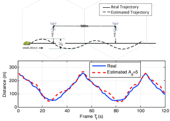
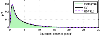
We first validate proposition 1. The real and estimated trajectory of the mobile user are shown in Fig. 1(a). To model a mobile user moving along a road, the real trajectory is generated as a straight line whose minimum distance from the BSs is 150150150 m. To model the behavior of a mobile user who may frequently change lanes during the T๐‘‡T time slots, the estimated trajectory is generated as a cosine function with amplitude Ad=5subscript๐ด๐‘‘5A_{d}=5 m and cycle ฯ€=3.14๐œ‹3.14\pi=3.14 seconds. The large-scale channel gains are computed from the distance d๐‘‘d with the assumed path loss model. Then, the value of Adsubscript๐ด๐‘‘A_{d} can reflect the estimation errors of the user location, which leads to the estimation errors of the large-scale channel gains. The PDFs computed from (8) with the accurate and estimated large-scale channel gains are shown in Fig. 1(b), where the PDF obtained from estimated large-scale fading gains is with legend โ€œESTโ€. We also provide the histogram of the estimated large-scale fading gains obtained from simulation. The results indicate that the channel distribution fโ€‹(g)๐‘“๐‘”f(g) can be obtained from large-scale channel gains accurately even when the large-scale information are imperfect.
Refer to caption
(a) True and estimated trajectories and the corresponding distances
Refer to caption
(b) PDF of the equivalent channel gains
Figure 1: PDF of gtsuperscript๐‘”๐‘กg^{t} with accurate and estimated large-scale fading gains for the true and estimated trajectories, Ts=100subscript๐‘‡๐‘ 100T_{s}=100.

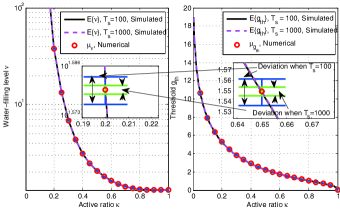
To validate (9) and proposition 2, we simulate the mean values of threshold gthsubscript๐‘”thg_{\rm th} and water-filling level ฮฝ๐œˆ\nu with different ฮบ๐œ…\kappa, and compare with ฮผgthsubscript๐œ‡subscript๐‘”th\mu_{g_{\rm th}} and ฮผฮฝsubscript๐œ‡๐œˆ\mu_{\nu} numerically obtained from (9) and (14) in Fig. 2(a) and 2(b). We also provide the simulated standard deviations of the estimated threshold and water-filling level when the numbers of time slots in each frame are respectively Ts=100subscript๐‘‡๐‘ 100T_{s}=100 and Ts=1000subscript๐‘‡๐‘ 1000T_{s}=1000, as shown with the blue and green curves in the magnified window. In Table I, we further provide the deviation of gthโˆ—subscriptsuperscript๐‘”thg^{*}_{\rm th} from ฮผgthโˆ—subscript๐œ‡subscriptsuperscript๐‘”th\mu_{g^{*}_{\rm th}} and ฮฝโˆ—superscript๐œˆ\nu^{*} from ฮผฮฝโˆ—subscript๐œ‡superscript๐œˆ\mu_{\nu^{*}}. It can be seen that the deviation from the mean value is small. Considering that in practice the large-scale channel gains vary in the scale of second and the small-scale channel gains change in the scale of milliseconds, this result indicates that the threshold and water-filling level can be estimated with the large-scale channel gains accurately.
Refer to caption
Figure 2: Simulated and numerically obtained threshold and water-filling level.

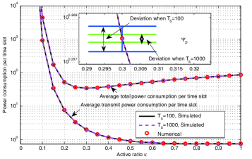
To validate proposition 3, we simulate the mean value of the transmit power per time slot ฮจpsubscriptฮจ๐‘\Psi_{p} and the total power consumption per time slot ฮฉฮฉ\Omega, and compare with analytical results ฮผฮจpsubscript๐œ‡subscriptฮจ๐‘\mu_{\Psi_{p}} and ฮผฮฉsubscript๐œ‡ฮฉ\mu_{\Omega} in Fig. 3. We can see that the analytical results perfectly match the simulated results. In the magnified window, we show the deviation of ฮจpsubscriptฮจ๐‘\Psi_{p} from its mean value when given ฮบ๐œ…\kappa, which is very small and decreases when Tssubscript๐‘‡๐‘ T_{s} increases. This suggests that ฮฉฮฉ\Omega can be estimated with large-scale channel gains accurately. Moreover, ฮฉฮฉ\Omega first decreases and then increases with ฮบ๐œ…\kappa, which validates that there exists optimal active ratio ฮบโˆ—superscript๐œ…\kappa^{*} minimizing the total power consumption and can be found by setting โˆ‚ฮฉ/โˆ‚ฮบ|ฮบ=ฮบโˆ—=0evaluated-atฮฉ๐œ…๐œ…superscript๐œ…0\partial\Omega/\partial\kappa|_{\kappa=\kappa^{*}}=0.

Refer to caption
Figure 3: Power consumption per time slot.
TABLE I: Deviation of the Optimal Water-filling Level and Threshold from Mean Value Estimation
Deviation Ts=100subscript๐‘‡๐‘ 100T_{s}=100 Ts=1000subscript๐‘‡๐‘ 1000T_{s}=1000
|ฮฝโˆ—โˆ’ฮผฮฝโˆ—|/ฮผฮฝโˆ—superscript๐œˆsubscript๐œ‡superscript๐œˆsubscript๐œ‡superscript๐œˆ{|\nu^{*}-\mu_{\nu^{*}}|}/{\mu_{\nu^{*}}} <1%absentpercent1<1\% <0.3%absentpercent0.3<0.3\%
|gthโˆ—โˆ’ฮผgthโˆ—|/ฮผgthโˆ—subscriptsuperscript๐‘”thsubscript๐œ‡subscriptsuperscript๐‘”thsubscript๐œ‡subscriptsuperscript๐‘”th{|g^{*}_{\rm th}-\mu_{g^{*}_{\rm th}}|}/{\mu_{g^{*}_{\rm th}}} <3%absentpercent3<3\% <1%absentpercent1<1\%

V-B Evaluation of the Energy Consumption

To show the impact of only using future large-scale channel gains on the energy-saving predictive resource allocation, we have simulated the following methods.

  • โ€ข

    SE-maximizing only with gtsuperscript๐‘”๐‘กg^{t} (with legend โ€œSEโ€): The closest BS serves the user with the maximal transmit power, which can maximize the spectrum efficiency (SE) in each time slot [5].

  • โ€ข

    EE-maximizing only with gtsuperscript๐‘”๐‘กg^{t} (with legend โ€œEEโ€): The closest BS serves the user with the optimized transmit power to maximize the EE in each time slot [5].

  • โ€ข

    Power allocation with perfect future channel information (with legend โ€œUBโ€): The closest BS allocates transmit power using (5) with ฮฝโˆ—superscript๐œˆ\nu^{*} and gthโˆ—superscriptsubscript๐‘”thg_{\rm th}^{*}, which consumes minimal consumption to convey the B๐ตB bits before the deadline with duration Tโ€‹ฮ”t๐‘‡subscriptฮ”๐‘กT\Delta_{t}.

  • โ€ข

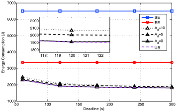
    Power allocation with future large-scale channel information (with legend โ€œAdsubscript๐ด๐‘‘A_{d}โ€): Considering that Tssubscript๐‘‡๐‘ T_{s} is finite in the simulation, we use the conservative way to estimate the water-filling level and threshold with the large-scale channel gains in order to complete the transmission of the B๐ตB bits during the T๐‘‡T time slots. Specifically, when Ad=0subscript๐ด๐‘‘0A_{d}=0, the BS allocates transmit power by using the estimated water-filling level and threshold in (IV-B) with perfect future large-scale channel information. When Ad=5subscript๐ด๐‘‘5A_{d}=5 and Ad=10subscript๐ด๐‘‘10A_{d}=10, the BS allocates power with (IV-B) by using the estimated future large-scale channel information.

If the B๐ตB bits can not be transmitted before the deadline with duration Tโ€‹ฮ”t๐‘‡subscriptฮ”๐‘กT\Delta_{t}, the remaining bits will be transmitted with the maximal transmit power.

In Fig. 4, we provide the energy consumed by different methods for transmitting the B๐ตB bits during the T๐‘‡T time slots. It can be seen that knowing the accurate large-scale channel information can achieve almost the same performance as knowing all the future channel information. Inaccurate large-scale channel information leads to more energy to transmit the B๐ตB bits, as shown in the magnified window, but the increased energy is not significant. Without exploiting the future large-scale channel information, the โ€œSEโ€ and โ€œEEโ€ methods consume much more energy to transmit the B๐ตB bits in duration Tโ€‹ฮ”t๐‘‡subscriptฮ”๐‘กT\Delta_{t}. Again, this validates that the large-scale channel information plays the key role on the energy-saving predictive resource allocation.
Refer to caption
Figure 4: Energy consumption vs. deadline, Ts=100subscript๐‘‡๐‘ 100T_{s}=100.

VI Conclusion

In this paper, we strived to show that large-scale channel information plays the key role on predictive resource allocation for delay tolerant services. Toward this goal, we formulated a time slot scheduling and power allocation problem minimizing the total energy consumed for conveying a given number of bits before a long deadline, where the large and small-scale channel gains are perfectly known for all time slots. We showed that only the water-filling level and threshold in the optimal solution contains future information, which can be estimated accurately with large-scale channel gains when the small-scale channels in each frame are ergodic. Simulation results validated our analysis and showed that the estimation errors of the large-scale channel gains have little impact on energy saving.

Appendix A Proof of proposition 1

Without loss of generality, we assume that the values of large-scale fading gains ฮฑj,j=1,โ€ฆ,Tfformulae-sequencesuperscript๐›ผ๐‘—๐‘—1โ€ฆsubscript๐‘‡๐‘“\alpha^{j},j=1,\ldots,T_{f} are within a range of [ฮฑmin,ฮฑmax]subscript๐›ผsubscript๐›ผ[\alpha_{\min},\alpha_{\max}]. We divided the range into Q๐‘„Q intervals as ฮด1,โ€ฆ,ฮดQsubscript๐›ฟ1โ€ฆsubscript๐›ฟ๐‘„\delta_{1},\ldots,\delta_{Q}, where ฮดq=[ฮฑmin+(qโˆ’1)โ€‹ฮด,ฮฑmin+qโ€‹ฮด]subscript๐›ฟ๐‘žsubscript๐›ผ๐‘ž1๐›ฟsubscript๐›ผ๐‘ž๐›ฟ\delta_{q}=[\alpha_{\min}+(q-1)\delta,\alpha_{\min}+q\delta], and ฮด=(ฮฑmaxโˆ’ฮฑmin)/Q๐›ฟsubscript๐›ผsubscript๐›ผ๐‘„\delta=(\alpha_{\max}-\alpha_{\min})/Q. The number of ฮฑj,j=1,โ€ฆ,Tfformulae-sequencesuperscript๐›ผ๐‘—๐‘—1โ€ฆsubscript๐‘‡๐‘“\alpha^{j},j=1,\ldots,T_{f} whose values are within the interval ฮดqsubscript๐›ฟ๐‘ž\delta_{q} is denoted as xqsubscript๐‘ฅ๐‘žx_{q}. Since each frame contains Tssubscript๐‘‡๐‘ T_{s} time slots with the same large-scale fading gain, the number of ฮฑj,j=1,โ€ฆ,Tformulae-sequencesuperscript๐›ผ๐‘—๐‘—1โ€ฆ๐‘‡\alpha^{j},j=1,\ldots,T whose values are within the interval ฮดqsubscript๐›ฟ๐‘ž\delta_{q} is Tsโ€‹xqsubscript๐‘‡๐‘ subscript๐‘ฅ๐‘žT_{s}x_{q}.

Consider a sequence of i.i.d random variables ฮฒn,n=1,โ€ฆ,Tsโ€‹Tfformulae-sequencesuperscript๐›ฝ๐‘›๐‘›1โ€ฆsubscript๐‘‡๐‘ subscript๐‘‡๐‘“\beta^{n},n=1,\ldots,T_{s}T_{f}, whose probability mass function is Prโ€‹(ฮฒn=ฮฑj)=1Tf,j=1,โ€ฆ,Tfformulae-sequencePrsuperscript๐›ฝ๐‘›superscript๐›ผ๐‘—1subscript๐‘‡๐‘“๐‘—1โ€ฆsubscript๐‘‡๐‘“{\rm Pr}(\beta^{n}=\alpha^{j})=\frac{1}{T_{f}},j=1,\ldots,T_{f}. Then, the probability that the value of ฮฒnsuperscript๐›ฝ๐‘›\beta^{n} is within the interval of ฮดqsubscript๐›ฟ๐‘ž\delta_{q} is Prโ€‹(ฮฒnโˆˆฮดq)=xq/TfPrsuperscript๐›ฝ๐‘›subscript๐›ฟ๐‘žsubscript๐‘ฅ๐‘žsubscript๐‘‡๐‘“{\rm Pr}(\beta^{n}\in\delta_{q})=x_{q}/T_{f}. When Tsโ†’โˆžโ†’subscript๐‘‡๐‘ T_{s}\to\infty, based on the Borelโ€™s law of large numbers, the number of ฮฒnsuperscript๐›ฝ๐‘›\beta^{n} within the interval of ฮดqsubscript๐›ฟ๐‘ž\delta_{q} (denoted as zqsubscript๐‘ง๐‘žz_{q}) approaches its average number, i.e., limTsโ€‹Tfโ†’โˆžzq=๐”ผโ€‹{zq}=Prโ€‹(ฮฒnโˆˆฮดq)โ€‹Tsโ€‹Tf=Tsโ€‹xqsubscriptโ†’subscript๐‘‡๐‘ subscript๐‘‡๐‘“subscript๐‘ง๐‘ž๐”ผsubscript๐‘ง๐‘žPrsuperscript๐›ฝ๐‘›subscript๐›ฟ๐‘žsubscript๐‘‡๐‘ subscript๐‘‡๐‘“subscript๐‘‡๐‘ subscript๐‘ฅ๐‘ž\lim_{T_{s}T_{f}\to\infty}z_{q}={\mathbb{E}}\{z_{q}\}={\rm Pr}(\beta^{n}\in\delta_{q})T_{s}T_{f}=T_{s}x_{q}. Therefore, the set {ฮฒn,n=1,โ€ฆ,Tsโ€‹Tf}formulae-sequencesuperscript๐›ฝ๐‘›๐‘›1โ€ฆsubscript๐‘‡๐‘ subscript๐‘‡๐‘“\{\beta^{n},n=1,\ldots,T_{s}T_{f}\} has the same elements as the large-scale fading gains of all the time slots but with different orders.

Further considering that the small-scale fading gains โ€–๐กtโ€–2,t=1โ€‹โ€ฆ,Tformulae-sequencesuperscriptnormsuperscript๐ก๐‘ก2๐‘ก1โ€ฆ๐‘‡\|{\bf h}^{t}\|^{2},t=1\ldots,T are i.i.d., the set of equivalent channel gains {gt=ฮฑโŒˆtTsโŒ‰โ€‹โ€–๐กtโ€–2/ฯƒ2,t=1,โ€ฆ,T}formulae-sequencesuperscript๐‘”๐‘กsuperscript๐›ผ๐‘กsubscript๐‘‡๐‘ superscriptnormsuperscript๐ก๐‘ก2superscript๐œŽ2๐‘ก1โ€ฆ๐‘‡\{g^{t}=\alpha^{\lceil\frac{t}{T_{s}}\rceil}\|{\bf h}^{t}\|^{2}/\sigma^{2},t=1,\ldots,T\} are the same as {ฮฒnโ€‹โ€–๐กtโ€–2/ฯƒ2,n=1โ€‹โ€ฆ,T,t=1โ€‹โ€ฆ,T}formulae-sequencesuperscript๐›ฝ๐‘›superscriptnormsuperscript๐ก๐‘ก2superscript๐œŽ2๐‘›1โ€ฆ๐‘‡๐‘ก1โ€ฆ๐‘‡\{\beta^{n}\|{\bf h}^{t}\|^{2}/\sigma^{2},n=1\ldots,T,t=1\ldots,T\}. Therefore, the PDF of gโ‰œฮฒnโ€‹โ€–๐กtโ€–2/ฯƒ2โ‰œ๐‘”superscript๐›ฝ๐‘›superscriptnormsuperscript๐ก๐‘ก2superscript๐œŽ2g\triangleq\beta^{n}\|{\bf h}^{t}\|^{2}/\sigma^{2} can be derived as

fโ€‹(g)=limฮ”โ†’0Prโ€‹(g<ฮฒnโ€‹โ€–๐กtโ€–2ฯƒ2โ‰คg+ฮ”)ฮ”.๐‘“๐‘”subscriptโ†’ฮ”0Pr๐‘”superscript๐›ฝ๐‘›superscriptnormsuperscript๐ก๐‘ก2superscript๐œŽ2๐‘”ฮ”ฮ”\displaystyle\!\!\!\!f(g)=\textstyle\lim\limits_{\Delta\to 0}\frac{{\rm Pr}(g<\frac{\beta^{n}\|{\bf h}^{t}\|^{2}}{\sigma^{2}}\leq g+\Delta)}{\Delta}. (21)

Because โ€–๐กtโ€–2superscriptnormsuperscript๐ก๐‘ก2\|{\bf h}^{t}\|^{2} follows Gamma distribution with PDF in (7), (21) can be further derived as

limฮ”โ†’0Prโ€‹(g<ฮฒnโ€‹โ€–๐กtโ€–2ฯƒ2โ‰คg+ฮ”)ฮ”subscriptโ†’ฮ”0Pr๐‘”superscript๐›ฝ๐‘›superscriptnormsuperscript๐ก๐‘ก2superscript๐œŽ2๐‘”ฮ”ฮ”\displaystyle\textstyle\lim\limits_{\Delta\to 0}\frac{{\rm Pr}(g<\frac{\beta^{n}\|{\bf h}^{t}\|^{2}}{\sigma^{2}}\leq g+\Delta)}{\Delta}
=\displaystyle= limฮ”โ†’0โˆ‘j=1TfPrโ€‹(ฮฒn=ฮฑj)โ€‹Prโ€‹(ฯƒ2ฮฑjโ€‹g<โ€–๐กtโ€–2โ‰คฯƒ2ฮฑjโ€‹(g+ฮ”))ฮ”subscriptโ†’ฮ”0superscriptsubscript๐‘—1subscript๐‘‡๐‘“Prsuperscript๐›ฝ๐‘›superscript๐›ผ๐‘—Prsuperscript๐œŽ2superscript๐›ผ๐‘—๐‘”superscriptnormsuperscript๐ก๐‘ก2superscript๐œŽ2superscript๐›ผ๐‘—๐‘”ฮ”ฮ”\displaystyle\textstyle\lim\limits_{\Delta\to 0}\frac{\sum_{j=1}^{T_{f}}{\rm Pr}(\beta^{n}=\alpha^{j}){\rm Pr}({\frac{\sigma^{2}}{\alpha^{j}}g}<\|{\bf h}^{t}\|^{2}\leq{\frac{\sigma^{2}}{\alpha^{j}}(g+\Delta)})}{\Delta}
=\displaystyle= 1Tfโ€‹โˆ‘j=1Tffhโ€‹(ฯƒ2ฮฑjโ€‹g),1subscript๐‘‡๐‘“superscriptsubscript๐‘—1subscript๐‘‡๐‘“subscript๐‘“โ„Žsuperscript๐œŽ2superscript๐›ผ๐‘—๐‘”\displaystyle\textstyle\frac{1}{T_{f}}\sum_{j=1}^{T_{f}}f_{h}(\frac{\sigma^{2}}{\alpha^{j}}g), (22)

which can be expressed as (8).

References

  • [1] H.ย Abou-zeid and H.ย Hassanein, โ€œPredictive green wireless access: exploiting mobility and application information,โ€ IEEE Wireless Commun., vol.ย 20, no.ย 5, pp. 92โ€“99, Oct. 2013.
  • [2] H.ย Abou-Zeid and H.ย S. Hassanein, โ€œToward green media delivery: location-aware opportunities and approaches,โ€ IEEE Wireless Commun., vol.ย 21, no.ย 4, pp. 38โ€“46, Aug. 2014.
  • [3] H.ย Abou-zeid, H.ย Hassanein, and S.ย Valentin, โ€œEnergy-efficient adaptive video transmission: Exploiting rate predictions in wireless networks,โ€ IEEE Trans. Veh. Technol., vol.ย 63, no.ย 5, pp. 2013โ€“2026, June 2014.
  • [4] M.ย Drรคxler, P.ย Dreimann, and H.ย Karl, โ€œAnticipatory power cycling of mobile network equipment for high demand multimedia traffic,โ€ in IEEE GREENCOM, 2014.
  • [5] C.ย Yao, C.ย Yang, and Z.ย Xiong, โ€œPower-saving resource allocation by exploiting the context information,โ€ in IEEE PIMRC, 2015.
  • [6] C.ย Park, Y.ย Seo, K.ย Park, and Y.ย Lee, โ€œThe concept and realization of context-based content delivery of NGSON,โ€ IEEE Commun. Mag., vol.ย 50, no.ย 1, pp. 74โ€“81, Jan. 2012.
  • [7] I.ย Skog and P.ย Handel, โ€œIn-car positioning and navigation technologiesโ€“a survey,โ€ IEEE Trans. Intell. Transportation Sys., vol.ย 10, no.ย 1, pp. 4โ€“21, March 2009.
  • [8] Z.ย Lu and G.ย deย Veciana, โ€œOptimizing stored video delivery for mobile networks: The value of knowing the future,โ€ in IEEE INFOCOM, April 2013, pp. 2706โ€“2714.
  • [9] H.ย Riiser, T.ย Endestad, P.ย Vigmostad, C.ย Griwodz, and P.ย Halvorsen, โ€œVideo streaming using a location-based bandwidth-lookup service for bitrate planning,โ€ ACM Trans. Multimedia Comput. Commun. Appl., vol.ย 8, no.ย 3, pp. 24:1โ€“24:19, Aug. 2012.
  • [10] H.ย Abou-zeid, H.ย Hassanein, Z.ย Tanveer, and N.ย AbuAli, โ€œEvaluating mobile signal and location predictability along public transportation routes,โ€ in IEEE WCNC, 2015.
  • [11] R.ย R. Bahadur, โ€œA note on quantiles in large samples,โ€ The Annals of Mathematical Statistics, vol.ย 37, no.ย 3, pp. pp. 577โ€“580, June 1966.
  • [12] TR 36.814 V1.2.0, โ€œFurther Advancements for E-UTRA Physical Layer Aspects (Release 9),โ€ 3GPP, June 2009.
  • [13] G.ย Auer, V.ย Giannini, C.ย Desset, and e.ย I.ย Godor, โ€œHow much energy is needed to run a wireless network?โ€ IEEE Wireless Commun., vol.ย 18, no.ย 5, pp. 40โ€“49, Oct. 2011.