Systematic effects from an ambient-temperature, continuously-rotating half-wave plate

Abstract

We present an evaluation of systematic effects associated with a continuously-rotating, ambient-temperature half-wave plate (HWP) based on two seasons of data from the Atacama B-Mode Search (ABS) experiment located in the Atacama Desert of Chile. The ABS experiment is a microwave telescope sensitive at 145 GHz. Here we present our in-field evaluation of celestial (CMB plus galactic foreground) temperature-to-polarization leakage. We decompose the leakage into scalar, dipole, and quadrupole leakage terms. We report a scalar leakage of $\sim 0.01\%$, consistent with model expectations and an order of magnitude smaller than other CMB experiments have reported. No significant dipole or quadrupole terms are detected; we constrain each to be $<0.07$% (95% confidence), limited by statistical uncertainty in our measurement. Dipole and quadrupole leakage at this level lead to systematic error on $r\lesssim 0.01$ before any mitigation due to scan cross-linking or boresight rotation. The measured scalar leakage and the theoretical level of dipole and quadrupole leakage produce systematic error of $r<0.001$ for the ABS survey and focal-plane layout before any data correction such as so-called deprojection. This demonstrates that ABS achieves significant beam systematic error mitigation from its HWP and shows the promise of continuously-rotating HWPs for future experiments.

I Introduction

Precise measurements of the Cosmic Microwave Background (CMB) polarization provide a unique window into the physics of the very early universe, where quantum-gravitational effects are expected to play an important role. A primordial gravitational-wave background (GWB) would leave a unique odd-parity “B-mode” pattern in the CMB polarization.Seljak and Zaldarriaga (1997); Kamionkowski, Kosowsky, and Stebbins (1997) Many models of inflation predict an observable GWB.Kamionkowski and Kovetz (2015) Its amplitude, as imprinted in the CMB polarization, is a direct measure of the energy scale of inflation. A detection of gravitational-wave-induced B-mode polarization in the CMB would provide compelling evidence for inflation and a rare glimpse into physics at ultra-high energies. The level of B-modes is parametrized by the tensor-to-scalar ratio, $r$, which is currently constrained to be $<0.07$ (95% confidence).Array and BICEP2 Collaborations (2015)

CMB polarization experiments face a daunting task as the level of the B-mode polarization is well below the level of unpolarized foregrounds. This makes systematic errors due to temperature-to-polarization leakage particularly detrimental. Polarization modulators offer a means of separating the polarized signal of interest from these unpolarized foregrounds. Many polarization modulation schemes exist Dicke (1946); Jarosik et al. (2003); Farese et al. (2004); Barkats et al. (2005); QUIET Collaboration et al. (2012a); Bersanelli et al. (2010); Stefanescu (2006); O’dell et al. (2003); Leitch et al. (2005); Padin et al. (2002); Chen et al. (2009); Moyerman et al. (2013), and a rapidly-rotating half-wave plate (HWP)Jones and Klebe (1988); Platt et al. (1991); Leach et al. (1991); Johnson et al. (2007); Ruhl (2008); Kusaka, Essinger-Hileman et al. (2014); Reichborn-Kjennerud et al. (2010); Ritacco et al. (2015) is one of the most promising. One of the key advantages of HWP modulation is that it allows single polarization-sensitive detectors to act as complete $Q/U$ polarimeters. Without modulation, experiments gain polarization sensitivity by differencing the output of pairs of detectors with sensitivity to orthogonal linear polarizations; however, pair differencing can cause significant temperature-to-polarization leakage if, for example, the pair of detectors has mismatched beams.Shimon et al. (2008) The BICEP2 and Keck Array teams estimate that their deprojection analysis technique reduces $I\rightarrow Q/U$ leakage by a factor of ten or more in their maps, to the $r=0.003$ level. BICEP2 and Keck Array Collaborations (2015a) Using a rapidly-rotating HWP eliminates the need for beam differencing and reduces the requirements on analysis techniques for removing any residual leakage contamination.

The Atacama B-Mode Search (ABS) experiment consists of 240 feedhorn-coupled bolometric polarimeters observing at 145 GHz with a rapidly-rotating, ambient-temperature HWP at the entrance aperture near a stop.Essinger-Hileman et al. (2009); Appel (2012); Essinger-Hileman (2011); Parker (2015); Visnjic (2013) Having the modulator as the first optical element in the system allows clear separation of instrumental polarization from celestial polarization; however, we note that the modeling presented below does not require the HWP to be at a stop, allowing straightforward application to systems such as those of POLARBEAR Suzuki et al. (2014) and the Atacama Cosmology Telescope. Niemack and ACTPol Collaboration (2013); Henderson et al. (2015) The HWP is made of single-crystal, $\alpha$-cut sapphire 330 mm in diameter and 3.15 mm thick. It is designed to work at 145 GHz. Sapphire has ordinary and extraordinary indices of refraction of $3.068\pm 0.003$ and $3.402\pm 0.003$, respectively. Parshin (1994) It is anti-reflection (AR) coated with 305 $\mu$m of Rogers RT/Duroid 6002,Visnjic (2013) a glass-reinforced PTFE laminate with a refractive index of $1.715\pm 0.012$. An air-bearing system allows the HWP to rotate at a stable frequency of 2.55 Hz. Porous graphite pads are placed around an aluminum rotor at three points on its circumference. Compressed air is forced through the graphite to float the rotor with almost no friction. An incremental encoder disc with an index to mark the zero point is used to read out the HWP angle with $2.4^{\prime}$ resolution.

The detectors for ABS were fabricated in two separate batches, which we label A and B, with half of the detectors in each batch. Due to an unexpected change in the microstrip dielectric constant between fabrications, batch B has a bandpass shifted up by $\sim 12$ GHz. The HWP is optimized for the bandpass of batch A, which carries approximately 90% of the statistical weight in the maps. The two batches of detectors are in separate halves of the focal plane, but both have detectors across the full range of radii from the center, which is relevant for comparison to the model.

The ABS HWP allows for separation of unpolarized atmospheric fluctuations, unpolarized ground pickup, and instrumental polarization from celestial polarization. In a companion paper,Kusaka, Essinger-Hileman et al. (2014) we demonstrated the ability of ABS to reject atmospheric fluctuations at better than 30 dB at 2 mHz. Here we present our in-field evaluation of celestial temperature-to-polarization leakage based on two seasons of observations. We break the leakage down into scalar, dipole, and quadrupole termsShimon et al. (2008) (see Figure 1) and investigate their effects on the power spectra from ABS. This parametrization is similar to the differential gain, pointing, and ellipticity in beam subtraction experiments, which we compare to in Section IV. In Section II we consider systematics associated with the beam profile and model expectations of their levels and functional forms. We characterize the scalar leakage in ABS in Section III and higher-order terms in Section IV, along with their impact on constraints on $r$. We conclude in Section V.

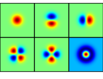
Figure 1: Monopole (“scalar”, top left), dipole (top middle and right), quadrupole (bottom left and middle), and differential width (bottom right) functions used to expand the modulated beam. In these maps, red and blue envelopes correspond to positive and negative leakages, respectively. The HWP does not induce differential width beam distortions. The functions are defined in terms of Gauss-Hermite functions, as in Equation 15.

II Description of systematic effect associated with the beam profile

The ABS data are demodulated in order to separate polarized from unpolarized emission.Kusaka, Essinger-Hileman et al. (2014) The HWP modulates incoming linear polarization at four times its rotation frequency $f_{m}$. The resulting data depend on the input Stokes parameters $(I,Q,U)$ and HWP angle, $\chi$, as

$$d_{m}=I+\varepsilon\mbox{Re}\left[(Q+iU)m(\chi)\right]+A(\chi)+\mathcal{N},$$ (1)

where $m(\chi)\equiv\exp{\left(-i4\chi\right)}$ is the modulation function, $A(\chi)$ is a HWP synchronous signal, $\varepsilon$ is the polarization modulation efficiency, and $\mathcal{N}$ is a noise term. We describe $A(\chi)$ in terms of its two dominant components

$$A(\chi)=A_{0}(\chi)+\lambda(\chi)I,$$ (2)

where $A_{0}(\chi)$ is independent of sky intensity, and the second term corresponds to conversion of unpolarized sky signal to modulated polarized light. Both components can be expanded as Fourier series in $\chi$, with the largest component in the $\sin 2\chi$ and $\cos 2\chi$ terms, corresponding to modulation in the detector timestreams at $2f_{m}$. Here we focus on the smaller $4f_{m}$ components, which cause leakage into the polarized signal of interest. (The $2f_{m}$ components can be used to assess data quality. Simon et al. (2015)) The $4f_{m}$ components arise from reflection-induced polarization being rotated, and thus modulated, by the HWP. Thus temperature-to-polarization leakage systematics increase with increasing angle of incidence, going to zero at normal incidence.

By multiplying the timestream by the complex conjugate of the modulation function and lowpass filtering below the modulation frequency, we create a complex-valued demodulated timestream:

$$\begin{split}d_{\bar{d}}=\frac{1}{2}\left(\varepsilon_{Q}Q+\lambda_{Q}I+\xi_{QU}U+A_{0}^{Q}\right)+\mathcal{N}^{Re}+\\ \frac{i}{2}\left(\varepsilon_{U}U+\lambda_{U}I+\xi_{UQ}Q+A_{0}^{U}\right)+i\mathcal{N}^{Im}\;.\end{split}$$ (3)

The real and imaginary parts of $d_{\bar{d}}$ are equivalent to $Q$ and $U$. Small $Q/U$ leakage terms have been added to this equation, denoted by $\xi_{QU}$ and $\xi_{UQ}$, which occur due to the same mechanism as temperature-to-polarization leakage, namely reflection-induced polarization. The total-power timestream is constructed separately by removing $A(\chi)$ and/or lowpass filtering the data. The $A(\chi)$ removal is done by binning all data in a certain time span (typically $\sim$1 hour) versus HWP angle $\chi$ and then subtracting this waveform from the data. We note that Eq. (3) ignores a very small effect where $I$ signal placed at around $4f_{m}$ frequency by scan modulation can remain as a residual temperature-to-polarization leakage. In contrast to the $\lambda_{Q}I$ and $\lambda_{U}I$ terms in Eq. (3), this effect couples two different angular scales; it is a leakage from intensity at small angular scales ($\sim 1\,\mathrm{arcmin}$ for the ABS scan speed) to degree-scale polarization. The effect is suppressed because of the beam size of the instrument and the fact that fine-resolution, or high-$\ell$, signal is small for CMB. We also note that this effect is not intrinsic to the instrument. If necessary, a map-making process can completely eliminate this systematic effect; a simple example of such a method is to take the difference between two orthogonal detectors in addition to the demodulation.

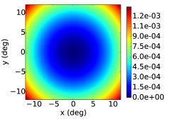
(a)

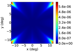
(b)

Figure 2: (a) Total leakage $\Lambda_{P}$ and (b) residual of Gauss-Hermite fit up to second order (monopole, dipole, and quadrupole terms) versus offset angle of a detector line-of-sight from instrument boresight for a $32^{\prime}$ FWHM Gaussian beam as estimated by the transfer-matrix modelEssinger-Hileman (2013) at 145 GHz. The colorbar indicates the integrated power normalized to that of an unpolarized input Gaussian beam. The majority of the leakage beam is captured in the monopole, dipole, and quadrupole terms.

We project the focal plane on the sky, and specify a position on the focal plane as well as the angular dependence of the instrument’s response using a spherical coordinate system, $\left(\theta,\phi\right)$. Here, $\theta$ is measured relative to the line of sight (LOS) corresponding to the center of the focal plane, and $\phi$ describes rotation about this LOS. The LOS to a detector $k$ is described by $\left(\theta_{k0},\phi_{k0}\right)$. The focusing optics of the instrument define the beam of each detector, $B_{k}(\theta_{k},\phi_{k})$, where $\left(\theta_{k},\phi_{k}\right)$ are defined relative to the detector LOS at $\left(\theta_{k0},\phi_{k0}\right)$. For this work we take the $B_{k}$ to be azimuthally symmetric Gaussians each with a full width at half maximum (FWHM) of $32^{\prime}$, a reasonable approximation for ABS. Since for ABS the HWP is the first element in the optical chain, the spread of rays impinging on the HWP for detector $k$ is described by that detector’s beam function in the global instrument coordinates. The HWP modifies incoming polarization differently depending upon the angle of rays going through it and those rays’ polarization state. These two effects combine to make $\varepsilon$ different functions for $Q$ and $U$ Stokes parameters, $\varepsilon_{Qk}(\theta_{k},\phi_{k})$ and $\varepsilon_{Uk}(\theta_{k},\phi_{k})$. The leakage beams, $\lambda_{Qk}$ and $\lambda_{Uk}$, similarly have angular dependence. Thus, Equation 3 is the result of an integral over $\theta_{k}$ and $\phi_{k}$.

To quantify systematic errors induced by the HWP, we seek to characterize (1) the beam-averaged magnitudes of $\lambda_{Q}$ and $\lambda_{U}$, denoted by $\Lambda_{Q}$ and $\Lambda_{U}$, which cause direct temperature-to-polarization (scalar) leakage, (2) the higher multipole terms in $\lambda_{Q}$ and $\lambda_{U}$; and, (3) how $\lambda_{Q}$ and $\lambda_{U}$ vary for detectors at different $\theta_{k0}$ and $\phi_{k0}$ across the focal plane. Another interesting property we can model is the small deviation of the polarized beams, $\varepsilon_{Qk}\left(\theta_{k},\phi_{k}\right)$ and $\varepsilon_{Uk}\left(\theta_{k},\phi_{k}\right)$, from Gaussians, which we will consider in a future paper. We define the total leakage as

$$\Lambda_{P}\equiv\sqrt{\Lambda_{Q}^{2}+\Lambda_{U}^{2}}.$$ (4)

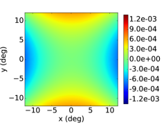
(a) I-to-Q leakage monopole, $a_{m0}$, for $\lambda_{Q}$, which is equivalent to $\Lambda_{Q}$. This is also the shape of $g_{I}^{4C}$ in Equation 13.

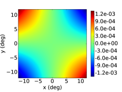
(b) I-to-U leakage monopole, $a_{m0}$, for $\lambda_{U}$, which is equivalent to $\Lambda_{U}$. This is also the shape of $g_{I}^{4S}$ in Equation 13.

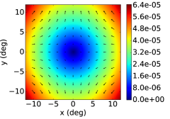
(c) I-to-Q dipole leakage. The color scale denotes total dipole leakage $\sqrt{a_{d1}^{2}+a_{d2}^{2}}$ for $\lambda_{Q}$. The arrows show the direction of the dipole, pointing toward the positive lobe of the dipole.

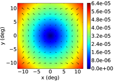
(d) I-to-U dipole term. The color scale denotes total dipole leakage $\sqrt{a_{d1}^{2}+a_{d2}^{2}}$ for $\lambda_{U}$. The arrows show the direction of the dipole, pointing toward the positive lobe of the dipole.

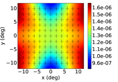
(e) I-to-Q quadrupole term. The color scale denotes total quadrupole leakage $\sqrt{a_{q1}^{2}+a_{q2}^{2}}$ for $\lambda_{Q}$. The solid (dashed) line shows the direction of the positive (negative) lobes of the quadrupole.

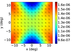
(f) I-to-U quadrupole term. The color scale denotes total quadrupole leakage $\sqrt{a_{q1}^{2}+a_{q2}^{2}}$ for $\lambda_{U}$. The solid (dashed) line shows the direction of the positive (negative) lobes of the quadrupole.

Figure 3: Modeled monopole, dipole, and quadrupole leakage terms versus offset angle from boresight for a $32^{\prime}$ FWHM Gaussian beam as estimated by the transfer-matrix modelEssinger-Hileman (2013) at 145 GHz for the ABS HWP. For definitions of the $a$ coefficients, see Equation 19. The colorbars indicate the integrated power in each component normalized to the unpolarized integrated input power.

Modeling beam systematic effects

To estimate the HWP beam systematic effects described above, a model of the HWP has been developed based upon the $4\times 4$ transfer-matrix method.Essinger-Hileman (2013) We can write the system response for ABS in matrix form, similar to a Mueller matrix, where the outputs of the data-reduction pipeline are total-power $\hat{I}$ and the real and imaginary parts of the demodulated timestream, Equation 3, which correspond to $\cos 4\chi$ and $\sin 4\chi$ components. The input is the Stokes vector, $\vec{S}=(I,Q,U,V)$. This means the system is described by an angle-dependent $4\times 3$ matrix, $\boldsymbol{M}_{\mathrm{total}}$, that maps the Stokes vector on the sky to the outputs of the data-reduction pipeline:

$$\left(\begin{array}[]{c}\hat{I}\\ \hat{Q}\\ \hat{U}\end{array}\right)=\int\left(\boldsymbol{M}_{\mathrm{total}}\cdot\vec{S}\right)d\Omega.$$ (5)

Here $\boldsymbol{M}_{\mathrm{total}}$ can be expanded in terms of the functions defined earlier,

$$\boldsymbol{M}_{\mathrm{total}} \equiv \hskip 48.0pt\left(\begin{array}[]{cccc}B_{k}&0&0&0\\ \lambda_{Qk}&\varepsilon_{Qk}&\xi_{QUk}&\zeta_{Qk}\\ \lambda_{Uk}&\xi_{UQk}&\varepsilon_{Uk}&\zeta_{Uk}\\ \end{array}\right)$$ (9)

$$= B_{k}\left(\theta_{k},\phi_{k}\right)\left(\begin{array}[]{cccc}1&0&0&0\\ g_{I}^{4C}&g_{Q}^{4C}&g_{U}^{4C}&g_{V}^{4C}\\ g_{I}^{4S}&g_{Q}^{4S}&g_{U}^{4S}&g_{V}^{4S}\\ \end{array}\right).$$ (13)

The nonzero terms of $M_{\mathrm{total}}$ depend on $\theta$ and $\phi$. The six angular response functions $g^{4C,4S}_{I,Q,U}(\theta,\phi)$ are calculated with the transfer-matrix model. The terms $g_{V}^{4C,4S}$ are expected to be negligible, as is celestial circular polarization, so we neglect $\zeta_{Qk}$ and $\zeta_{Qk}$ here. The model results are calculated at 145 GHz at the center of the ABS band. This frequency is relevant for systematic effects such as internal reflection caused by imperfect anti-reflection coating for off-axis incident rays. No band averaging is performed. The model describes how the HWP would couple infinite plane waves with incoming Stokes $I$, $Q$, and $U$ parameters to the real and imaginary parts of the demodulated timestream in the absence of the focusing optics.

Multiplying the $g$ functions by the beam yields $\lambda_{Qk}\left(\theta_{k},\phi_{k}\right)$ and $\lambda_{Uk}\left(\theta_{k},\phi_{k}\right)$ and the other terms in Equation 3. This amounts to decomposing the Gaussian beam at the HWP into a superposition of infinite plane waves. This approach ignores edge effects due to truncation of the beam by the telescope aperture, which is a valid approximation for ABS because the aperture is many, $\simeq 100$, wavelengths across.

Modeled leakage levels

We wish to characterize the impact of HWP beam systematics in a way that highlights the effects on final data quality. To this end, we perform an expansion of the beam into monopole (scalar), dipole, and quadrupole terms.Shimon et al. (2008); BICEP2 (2015) The expansion functions are shown in Figure 1. We focus here on the temperature-to-polarization leakage beams, $\lambda_{kQ},\lambda_{kU}$, which can be expanded into Gauss-Hermite functions as

$$\lambda_{k\{Q,U\}}(\theta_{k},\phi_{k})=\sum_{j=0}^{\infty}\sum_{i=0}^{\infty}s_{kij}f_{ij}(\theta_{k},\phi_{k}).\\$$ (14)

Here $s_{kij}$ are the fit coefficients and the normalized basis functions $f_{ij}(\theta,\phi)$ are

$$\begin{split}f_{ij}(\theta_{k},\phi_{k})=&\left(\frac{\exp{\left[-\theta_{k}^{2}/(2\sigma^{2})\right]}}{\sqrt{2^{i+j}i!j!\pi\sigma^{2}}}\right)\\ &\times H_{i}\left(\frac{\theta_{k}\cos\phi_{k}}{\sigma}\right)H_{j}\left(\frac{\theta_{k}\sin\phi_{k}}{\sigma}\right),\end{split}$$ (15)

where $\sigma=32^{\prime}/\sqrt{8\ln 2}$ is the Gaussian width of the beam and $H_{i}$ and $H_{j}$ are Hermite polynomials. The dominant effects on the data quality will come from the lower order, $i+j\leq 2$, terms for two reasons: (1) the higher-order terms are negligibly small and (2) we care most about leakage from local dipoles and quadrupoles, which will not average down as easily as the higher-order terms. A similar expansion can be done for the other beams, $\varepsilon_{Q}$, $\varepsilon_{U}$, $\xi_{QU}$, and $\xi_{UQ}$.

The lowest-order beam distortions can be written out explicitly, as

$$\begin{array}[]{rcccl}f_{m0}\left(\theta,\phi\right)&\equiv&f_{00}&=&1/(\sqrt{\pi\sigma^{2}})\exp{\left(-\frac{\theta^{2}}{2\sigma^{2}}\right)}\;,\\ f_{d1}\left(\theta,\phi\right)&\equiv&f_{10}&=&\sqrt{2}(\theta\cos\phi/\sigma)f_{00}\;,\\ f_{d2}\left(\theta,\phi\right)&\equiv&f_{01}&=&\sqrt{2}(\theta\sin\phi/\sigma)f_{00}\;,\\ f_{q1}\left(\theta,\phi\right)&\equiv&f_{11}&=&(\theta^{2}\sin 2\phi/\sigma^{2})f_{00}\;.\\ \end{array}$$ (16)

We identify $f_{m0}$ as the monopole (scalar) beam, $f_{d1}$ and $f_{d2}$ as the horizontal and vertical dipoles, respectively, and $f_{q1}$ as the cross-shaped quadrupole. The plus-shaped quadrupole is defined to be

$$f_{q2}\equiv(f_{20}-f_{02})/\sqrt{2}=\frac{\theta^{2}\cos 2\phi}{\sigma^{2}}f_{00},$$ (17)

and the differential width function is

$$f_{m1}\equiv(f_{20}+f_{02})/\sqrt{2}=\left(\frac{\theta^{2}}{\sigma^{2}}-1\right)f_{00}.$$ (18)

We define $a$ coefficients that are normalized versions of the $s$ coefficients in Eq. 14:

$$\begin{array}[]{rcl}a_{m0}&\equiv&s^{\text{leak}}_{00}/s^{\text{main}}_{00}\;,\\ a_{m1}&\equiv&(1/\sqrt{2})(s^{\text{leak}}_{20}+s^{\text{leak}}_{02})/s^{\text{main}}_{00}\;,\\ a_{d1}&\equiv&s^{\text{leak}}_{10}/s^{\text{main}}_{00}\;,\\ a_{d2}&\equiv&s^{\text{leak}}_{01}/s^{\text{main}}_{00}\;,\\ a_{q1}&\equiv&s^{\text{leak}}_{11}/s^{\text{main}}_{00}\;,\\ a_{q2}&\equiv&(1/\sqrt{2})(s^{\text{leak}}_{20}-s^{\text{leak}}_{02})/s^{\text{main}}_{00}\;.\\ \end{array}$$ (19)

Figure 2(a) summarizes the modeled ABS temperature-to-polarization leakage as a function of position on the focal plane; the color scale indicates the magnitude $\Lambda_{P}$. Figure 2(b) shows the residuals as a function of position on the focal plane after removing the scalar, dipole, and quadrupole terms from the modeled leakage. Figure 3 shows the modeled monopole, dipole, and quadrupole leakage beams for $I\rightarrow Q$ and $I\rightarrow U$, derived respectively from $\lambda_{Q}$ and $\lambda_{U}$. Specifically, Figure 3(a) (3(b)) show $a_{m0}$ for $\lambda_{Q}$ ($\lambda_{U}$) for each position $k$ in the focal plane, which is equal to $\Lambda_{Q}$ ($\Lambda_{U}$). It should be noted that $a_{m0}$ for $\lambda_{Q}$ ($\lambda_{U}$) is nearly exactly $g_{I}^{4C}$ ($g_{I}^{4S}$) in Equation 13, and this correspondence becomes exact as the beam width goes to zero. For later comparison to data, we construct an estimator of $\Lambda_{P}$ that is always positive in the model

$$\widetilde{\Lambda}_{P}=-\Lambda_{Q}\cos 2\phi-\Lambda_{U}\sin 2\phi$$ (20)

and an orthogonal function that is always zero

$$\widetilde{\Lambda}^{\bot}=\Lambda_{Q}\sin 2\phi-\Lambda_{U}\cos 2\phi.$$ (21)

Here $\phi=\phi_{k0}$ when $\widetilde{\Lambda}_{P}$ or $\widetilde{\Lambda}^{\bot}$ is calculated for a detector $k$.

Figures 3(c) and 3(d) show the magnitude of the two dipole terms $\sqrt{a_{d1}^{2}+a_{d2}^{2}}$ in the color scale with the direction of the dipole indicated by the overplotted arrows, for $\lambda_{Q}$ and $\lambda_{U}$, respectively. Finally, Figures 3(e) and 3(f) show the magnitude of the two quadrupole terms $\sqrt{a_{q1}^{2}+a_{q2}^{2}}$ in the color scale with the direction of the quadrupole indicated by the overplotted crosses for $\lambda_{Q}$ and $\lambda_{U}$, respectively. We do not plot the coefficient for the differential width function defined in Equation 18 as it is zero everywhere.

III Measurement of Scalar Leakage

We use $A(\chi)$, defined in Equation 2, to characterize the leakage $\Lambda_{P}$ (Equation 4). The function $A(\chi)$ is measured for each $\sim$one hour constant-elevation scan (CES) of the CMB. The terms with $\cos 4\chi$ and $\sin 4\chi$ dependence can be written as

$$A(\chi)=\left(\Lambda_{Q}I+A_{0}^{Q}\right)\cos 4\chi+\left(\Lambda_{U}I+A_{0}^{U}\right)\sin 4\chi+\cdots\>.$$ (22)

Note that we have switched to beam-averaged quantities in this equation. To determine $\Lambda_{Q}$ and $\Lambda_{U}$, we use the fact that the sky intensity $I$ changes with precipitable water vapor (PWV). We estimate the atmosphere contribution to the intensity for each CES from the elevation angle of the ABS telescope and the PWV measured by APEX.  To convert to temperature units, we use the ABS frequency bandpasses presented in our previous publicationSimon et al. (2014) and the ATM (atmospheric transmission at microwaves) modelPardo, Cernicharo, and Serabyn (2001) implemented as the AATM package.

Figure 4 shows an example of such a relation between the sky intensity $I$, and the amplitudes of the $\cos 4\chi$ and $\sin 4\chi$ terms. The slopes in this correlation plot correspond to the leakage coefficients $\Lambda_{Q}$ and $\Lambda_{U}$. We evaluate the statistical uncertainty by dividing the data into subsets, each corresponding to a period of a few weeks to months. The estimated leakage coefficients are consistent among the data subsets. From the variance of these subset estimates, we estimate the uncertainty on $\Lambda_{P}$ for each detector as 0.006% (0.007%) for group A (B) detectors.

Next, we compute $\tilde{\Lambda}_{P}$ (Eq. 20) from the measured $\Lambda_{Q}$ and $\Lambda_{U}$ and compare it to the estimates from the transfer-matrix model. As shown in Figure 5, the model correctly predicts that $\widetilde{\Lambda}_{P}$ increases with distance from boresight and that the orthogonal leakage $\widetilde{\Lambda}^{\bot}$ is consistent with zero. The data values of $\widetilde{\Lambda}_{P}$ are not forced to be positive and can in principle take negative values. The model also predicts the amplitude of $\widetilde{\Lambda}_{P}$ within a factor two. This overall agreement between the model prediction and the ABS data demonstrates that the transfer-matrix model will be a useful tool in designing future experiments. The factor two difference in amplitude could be due to uncertainties in the thickness, index of refraction, or absorptive loss of the HWP and its anti-reflection (AR) coating. For instance, the blue band in the figure shows the effect on the modeled leakage for the expected maximum $\pm$25 $\mu$m uncertainty in the anti-reflection coating thickness due to manufacturing tolerances. Similar levels of uncertainty can be attributed to thickness variation of the adhesive layer between the HWP and its anti-reflection coating.

Figure 6 presents a histogram of the leakage coefficients $\Lambda_{P}\equiv\sqrt{{\Lambda_{Q}}^{2}+{\Lambda_{U}}^{2}}$. Note that if every $\Lambda_{Q}$ and $\Lambda_{U}$ were drawn from distributions with zero mean and width $\sigma$, the histogram would not peak at zero. After correcting for this bias, the median value of the total leakage is $\Lambda_{P}=0.013\%$ (0.031%) for the detector group A (B). We put a conservative upper limit on the effective scalar leakage in ABS of

$$\Lambda_{P}<0.03\%\hskip 10.0pt(\text{magnitude method})$$ (23)

from these data, noting that the group A detectors dominate the statistical weight. The typical value of the scalar leakage, 0.013%, is considerably smaller than has been previously reported, as indicated in Table 2.

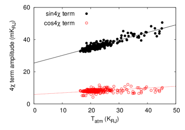
Figure 4: An example of the relation between the brightness temperature of the atmosphere and the amplitudes of the $\cos 4\chi$ and $\sin 4\chi$ terms in $A(\chi)$ for one of the ABS detectors. Each point in this plot corresponds to an $\sim$ hour-long CES. Note that we estimate the coefficients in temperature units (without converting to the CMB units appropriate for differential measurements near the peak of that blackbody).

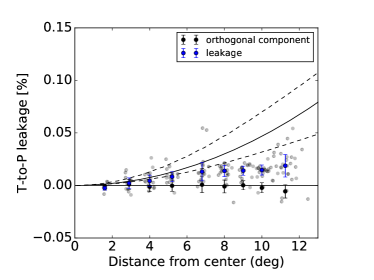
Figure 5: Intensity-to-polarization leakage, estimated using the $A(\chi)$ signal versus precipitable water vapor (PWV) described in the text, versus radial distance from the boresight for group A detectors. These detectors were chosen for this analysis, because they have well-measured and similar bandpasses. Each gray dot is the leakage $\widetilde{\Lambda}_{P}$ (defined in Equation 20) averaged over two seasons of observations for a single detector. We estimate the mean error for each of these points to be 0.006%. The blue dots are binned averages for groups of detectors at approximately the same focal plane radius, with the error bar the variance of the group. The black dots show the binned averages for $\widetilde{\Lambda}^{\bot}$, which are close to zero as predicted by the model. The solid black curve is the fiducial estimate from the transfer-matrix model with the dashed lines corresponding to uncertainty in the anti-reflection coating thickness of $\pm 25$ $\mu$m due to manufacturing tolerances.

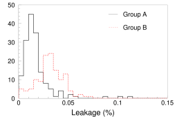
Figure 6: A histogram of the $T\rightarrow P$ leakage, defined as $\sqrt{{\Lambda_{Q}}^{2}+{\Lambda_{U}}^{2}}$. Each entry of this histogram corresponds to a detector. We note that this is a biased estimator due to the statistical error of the measurement; the level of the bias is estimated to be 0.009% (0.011%) for the group A (B) detectors. The median value of the leakage is 0.013% (0.031%) for group A (B).

Although estimating an upper limit on the leakage from estimates of $\Lambda_{P}$ is the more conservative approach, we can also provide a more direct estimate that circumvents the problem of bias in estimating a magnitude. We investigate the mean values of the leakage coefficients across the focal plane, finding $\bar{\Lambda}_{Q}$ = 0.005% ($-0.001$%) and $\bar{\Lambda}_{U}$ = 0.007% ($-0.003$%) for detectors from group A (B). We estimate the errors on these means as 0.003% for each case from the standard deviations of the distributions of $\Lambda_{Q}$ and $\Lambda_{U}$ for each detector group. We use the $2\sigma$ limit on $\sqrt{\left(\bar{\Lambda}_{Q}\right)^{2}+\left(\bar{\Lambda}_{U}\right)^{2}}$ from group A to provide a second estimate of the effective scalar leakage:

$$\Lambda_{P}<0.014\%\hskip 10.0pt(\text{mean value method})$$ (24)

Neglecting possible suppression of the systematic error by sky rotation and cancellation in averaging pixels across the focal plane, a leakage coefficient of 0.014% leads to systematic bias as small as a tensor-to-scalar ratio $r$ of 0.002–0.003 by taking the formalism of Shimon et. al. 2008Shimon et al. (2008). In order to assess the level of systematic-error mitigation from sky rotation and focal plane averaging, we perform an end-to-end pipeline simulation of ABS for season 1 and 2 observations, based on the detector-by-detector leakage coefficients predicted by our model (Fig. 3). Figure 9 shows the resultant estimate of the systematic bias. The bias is at a level of $r<0.001$ for angular scales of $\ell<100$. Sky rotation and the cancellation across the focal plane yield factors of $\sim 2$ and $\sim 5$, respectively, reduction of the systematic error in power. There is significant room for improvement in future experiments, because (1) ABS had a scan pattern that was not optimal for reducing systematic error via sky rotation, specifically for the monopole leakage; (2) ABS had a focal plane with highly non-uniform sensitivity, degrading the focal-plane cancellation; and (3) the ABS scan width was $\sim 7$ degrees, smaller than the focal plane diameter of $\sim 20$ degrees, again decreasing cancellation from focal-plane averaging. We also note that the average modeled scalar leakage is $\sim 0.022$%, while our data implies a smaller amplitude of 0.014% as can be seen in Fig. 5. If we scale the leakage by this factor, the bias on $r$ would decrease by a factor of $\simeq 2.5$ compared to Fig. 9.

IV Higher-Order Leakage: Dipole and Quadrupole

We now constrain the higher order terms in $\lambda_{Q}(\theta,\phi)$ and $\lambda_{U}(\theta,\phi)$. All the terms are consistent with zero, and thus we derive upper limits on the leakage coefficients $a_{d}$, $a_{q}$, and $a_{m1}$ based on the errors in our measurement. These constraints are obtained by making maps of Jupiter. An ideal polarization modulator without any polarization systematics would lead to a null signal in these polarization maps assuming Jupiter is unpolarized. For a non-ideal HWP, the angle-dependent leakage beams $\lambda_{Q}(\theta,\phi)$ and $\lambda_{U}(\theta,\phi)$ will appear in maps of an unpolarized source. Scalar leakage shows up as a spurious point source at the location of the unpolarized source, with the same shape as the total intensity beam shape. Higher-order terms show up as zero-mean patterns (e.g., dipole or quadrupole) in the maps.

We note that our constraints are robust against possible intrinsic polarization of Jupiter for two reasons. First, to a good approximation, polarization of Jupiter would only contribute to the monopole terms and the higher order terms are immune to the polarization of Jupiter. Second, we only put upper limits on the leakage coefficients and thus contribution from non-zero polarization of Jupiter would only make the limits more conservative.

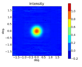
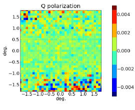
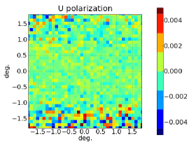
Figure 7: Stacked intensity and “polarization” maps of Jupiter for pod 4 detectors, one of the best-observed pixel groups. Left: intensity map of Jupiter, corresponding to the ABS intensity beam. Center and Right: Q and U “polarization” maps of Jupiter using demodulated data. The color scale is normalized such that the peak of the intensity map (left) is unity. The maps are for a group of 20 detectors near the center of the focal plane. Assuming Jupiter is unpolarized, we expect no signal when the HWP creates no spurious polarization. Note that these maps do not constitute a limit on the possible polarization of Jupiter; $\sim 30$ observations are coadded to create the maps in a manner to coherently add up possible instrumental polarization, but not necessarily to add the polarization of Jupiter.

For detectors from group A, we make stacked maps of multiple Jupiter observations for sets of ten neighboring pixels (20 detectors). Figure 7 presents an example of Jupiter maps for one of the best-calibrated sets (hereafter “pod 4”). This group is in a region $2^{\circ}-6^{\circ}$ from the center of the focal plane. To create these maps, some $\sim 30$ observations are stacked in co-azimuth vs. co-elevation coordinates, which coherently add up the $T\rightarrow P$ leakage beam but not necessarily add up possible intrinsic polarization of Jupiter. The left panel shows the total intensity beam. The center and right panels show the demodulated data maps. The maps are normalized such that the peak of the intensity map is unity. No spurious polarization is evident. We calculate two types of radial projections of the polarization maps by integrating over $\cos n\phi$ or $\sin n\phi$ to pick out dipole ($n=1$) and quadrupole ($n=2$) terms:

$$Q_{n}^{c[s]}(\theta) \equiv \int\mathrm{d}\phi Q(\theta,\phi)\cos n\phi[\sin n\phi]$$ (25)

$$U_{n}^{c[s]}(\theta) \equiv \int\mathrm{d}\phi U(\theta,\phi)\cos n\phi[\sin n\phi]$$ (26)

We note that the quadrupole terms are irreducible by sky rotation Hu, Hedman, and Zaldarriaga (2003) and thus among the most important sources of systematic error. Among the four quadrupole terms, $Q^{s}_{2}(\theta)$ and $U^{c}_{2}(\theta)$ lead to spurious $B$ modes, while $Q^{c}_{2}(\theta)$ and $U^{s}_{2}(\theta)$ result in spurious $E$ modes.

To compare these data with the prediction presented in Section II, we define the following radially-projected leakage beam templates for two monopoles ($f_{m0}$ and $f_{m1}$), dipole ($f_{d}$) and a quadrupole ($f_{q}$):

$$\begin{split}f_{m0}(\theta)&\equiv\frac{\sqrt{\pi\sigma^{2}}}{2\pi}\int\mathrm{d}\phi f_{m0}(\theta,\phi)\>,\\ f_{m1}(\theta)&\equiv\frac{\sqrt{\pi\sigma^{2}}}{2\pi}\int\mathrm{d}\phi f_{m1}(\theta,\phi)\>,\\ f_{d}(\theta)&\equiv\frac{\sqrt{\pi\sigma^{2}}}{2\pi}\int\mathrm{d}\phi\cos\phi\>f_{d1}(\theta,\phi)\>,\\ f_{q}(\theta)&\equiv\frac{\sqrt{\pi\sigma^{2}}}{2\pi}\int\mathrm{d}\phi\cos 2\phi\>f_{q2}(\theta,\phi)\>.\end{split}$$ (27)

The prefactors $\sqrt{\pi\sigma^{2}}$ are normalization factors such that the peak of the main beam is unity in the maps shown in Fig. 7. That is, this normalization allows us to directly obtain coefficients $a_{m0}$, $a_{m1}$, $a_{d1}$, $a_{d2}$, $a_{q1}$ and $a_{q2}$ by fitting the radially-averaged leakage maps (Eqs. 25 and 26) to these templates. For $P=Q,U$, fitting $f_{d}$ on $P_{1}^{c}$ ($P_{1}^{s}$) yields $a_{d1}$ ($a_{d2}$), and fitting $f_{q}$ on $P_{2}^{c}$ ($P_{2}^{s}$) yields $a_{q1}$ ($a_{q2}$). In the following, we treat $a_{d1}$ and $a_{d2}$ together as $a_{d}$ and $a_{q1}$ and $a_{q2}$ together as $a_{q}$, unless otherwise noted. We fit the templates and determine the coefficients one by one.

Figure 8 shows the monopole, dipole and quadrupole leakage components derived from the maps shown in the center and right panels of Figure 7 following Equations 25 and 26. The data are consistent with zero at the $\sim\,0.02$% level. The curves for templates are shown for comparison.

We note that these leakage beam templates are equivalent to those defined in Shimon, et al. 2008, Shimon et al. (2008) in describing a “two-beam” experiment which required beam differencing, in the limit of small leakages. Three of the four coefficients for the templates correspond to differential gain ($g$), differential pointing ($\rho$) and differential ellipticity ($e$) as $a_{m0}=g/2$, $a_{d}=\rho/(\sqrt{8}\sigma)$ and $a_{q}=e$. The differential beam width ($\mu$) and the coefficient $a_{m1}$ do not have the same template function shape. Further details are in Appendix A.

While none of the 12 amplitudes fitted show significant deviation from zero, the total $\chi^{2}$ to zero for the 12 amplitudes is 23 with 12 degrees of freedom. We consider this excess is likely to be because of an underestimate of the errors, which are empirically obtained. We thus conservatively place upper limits on these amplitudes using errors inflated by a factor of $\sqrt{23/12}=1.4$. The “pod 4” column in Table 1 shows the 2-$\sigma$ upper limits. We repeat the same analyses on another eight (of twelve) relatively well-calibrated groups of batch A detectors; the eight groups broadly distribute across the top half of the focal plane. Using the scatter among the eight groups, we estimate the error per group. We find no significant deviation from zero, with a total $\chi^{2}$ of 10.9 for 12 degrees of freedom. Thus, we put upper limits on these coefficients without inflating the errors here. The “others” column in Table 1 summarizes those limits. We note that these limits are more conservative than a usual 2-$\sigma$ limit in that we take the worst case among two (four) 2-$\sigma$ upper limits for monopole (dipole and quadrupole) amplitudes.

Taking the formalism of Shimon et. al. 2008Shimon et al. (2008) and neglecting possible systematic-error mitigation by sky rotation, we relate these upper limits to the systematic bias in B-mode power. The upper limits of the quadrupole and differential width terms correspond to $r=0.001$ or lower. The limit on the dipole term corresponds to $r\sim 0.003$ (0.01) for pod 4 (others). With an optimal scan strategy, sky rotation would mitigate the dipole systematics further. We also note that these limits are dominated by the uncertainties of our beam measurement, and the true values of the coefficients are expected to be lower. Figure 9 shows the expected bias based on typical values of the leakage coefficients from our model (Fig. 3), which are $2.9\times 10^{-5}$ and $1.4\times 10^{-6}$ for the dipole and quadrupole leakages, respectively. Here we neglect possible mitigation of the dipole leakage by sky rotation and focal plane cancellation. The bias is well below the level of a primordial gravitational wave signal with $r=0.001$ or gravitational lensing B modes.

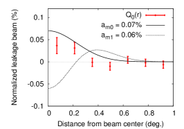
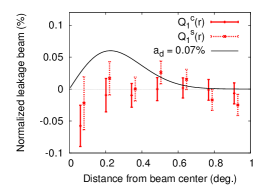
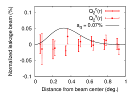
Figure 8: The radial averages of monopole, dipole, and quadrupole in Q polarization defined by Eq. (25) for the pod 4 maps shown in Fig. 7, center. Plotted curves correspond to example templates for monopole, dipole, and quadrupole terms with amplitudes that correspond to the upper limits shown in Table 1.

Table 1: Upper limits on the amplitudes of measured $I\rightarrow P$ leakage terms from analysis of stacked maps of Jupiter. Each row corresponds to a group of two (four) amplitudes for monopole (dipole and quadrupole) terms; the worst case of the two (four) 2-$\sigma$ upper limits are shown here. For the second monopole term, we present constraints on both $a_{m1}$ (see Equation 27) and the two-beamShimon et al. (2008) parameter $\mu$ since their template functions are different. The Pod 4 stacked maps are more sensitive than the “Others” maps, as explained in the text. Note that Section III provides a measurement of the scalar leakage which is more constraining than the limits in this table.

	Pod 4	Others
$|a_{m0}|$ (%)	$<0.07$	$<0.13$
$|a_{m1}|$ (%)	$<0.06$	$<0.09$
$\quad|\mu|$ (%)	$<0.05$	$<0.09$
$|a_{d}|$ (%)	$<0.07$	$<0.13$
$|a_{q}|$ (%)	$<0.07$	$<0.14$

Table 2: Published estimates of $I\rightarrow P$ leakage for various experiments. When quoted for two-beam experiments, the leakage estimates are converted to the Gauss-Hermite basis used here according to the prescriptions of Appendix A. For $|a_{m0}|$, we present the median value from measurements of $A(\chi)$ as detailed in Section III. Upper limits on higher-order beam terms are derived from Jupiter maps from Section IV.

	$|a_{m0}|$	$|\mu|$	$|a_{d}|$	$|a_{q}|$
	(%)	(%)	(%)	(%)
BICEPChiang et al. (2010)	$<1.1$	—	$0.5\pm 0.1$	—
BICEP2/KeckBICEP2 and Keck Array Collaborations (2015b)	1	$0.08\pm 0.4$	$0.64\pm 1.7$	$0.7\pm 1.2$
MAXIPOLJohnson et al. (2007)	1–4	—	—	—
QUIET QQUIET Collaboration et al. (2011)	0.2–1	—	0.1	0.1
QUIET WQUIET Collaboration et al. (2012b)	0.4	—	0.4	0.3
WMAPPage et al. (2007)	0.1	6–8	—	—
ABS	$0.013$	$<0.05$	$<0.07$	$<0.07$

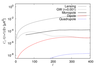
Figure 9: The level of $I\rightarrow P$ leakage systematic error for monopole, dipole, and quadrupole terms compared with the $BB$ power spectra of lensing and primordial gravitational waves (GW) with a tensor-to-scalar ratio $r=0.001$. The leakage coefficients are taken from the model shown in Fig. 3. We emphasize that these are the estimates before any correction (e.g., deprojection). For the monopole, we perform an end-to-end pipeline simulation of ABS for season 1 and 2 observations, yielding a level of systematics below $r=0.001$ for $\ell<100$. Note that the average amplitude of the coefficients from our model is $\sim 0.022$%, while our data implies a smaller amplitude of 0.014% as can be seen in Fig. 5. Taking the smaller amplitude implied by our data leads to a reduction in systematic error by a factor $\simeq 2.5$. For the dipole and quadrupole leakages, we take typical leakage values of $2.9\times 10^{-5}$ and $1.4\times 10^{-6}$, respectively, from the model (Fig. 3) and analytically calculate the systematic bias;Shimon et al. (2008) we neglect possible mitigation of the dipole leakage by sky rotation and focal plane cancellation. The bias is well below the levels of $r=0.001$ or the gravitational lensing B modes.

V Conclusion

We have demonstrated low temperature-to-polarization systematic errors from a continuously-rotating HWP in observing CMB polarization with the ABS instrument. Table 2 compares leakage results from ABS with other CMB experiments. Estimated levels of the ABS errors are presented using a transfer-matrix model.Essinger-Hileman (2013) The scalar leakage component is measured to be consistent with expectations, and we put a conservative upper limit on its magnitude of 0.01–0.03%. The model correctly predicts two trends found in the data: the increase of the leakage as a function of the distance of a pixel from the center of the focal plane, and the relation between the direction of the leakage polarization and the position of a pixel in the focal plane. The higher-order dipole and quadrupole terms are not detected, leading to upper limits on each of 0.07%. This is also consistent with expectations. Before any systematic error mitigation due to cross-linking or boresight rotation, the upper limits correspond to $r\lesssim 0.01$. The measured scalar leakage and the theoretical level of dipole and quadrupole leakage produce systematic error of $r<0.001$ for the ABS survey and focal-plane layout before any data correction such as so-called deprojection. Our study demonstrates the benefits of using a HWP for systematic error mitigation and the value of the transfer-matrix model as a tool for designing future experiments.

Appendix A Relation of Gauss-Hermite functions to beam-differencing experiments

We wish to convert between the Gauss-Hermite monopole, dipole, quadrupole basis used here and the differential gain, pointing, and ellipticity basis of Shimon et al. 2008. Shimon et al. (2008) The functions defined in Equations 16–18 can be related to the differential gain, differential beam width, differential pointing, and differential ellipticity for beam differencing experiments in the limit of small differences between the two beams. We note again that the differential beam width function, also a monopole term, is not induced by the HWP. An elliptical Gaussian offset from zero along the x axis can be denoted by

$$G(\theta,\phi;g,\sigma,e,\rho)\equiv\frac{g}{2\pi\sigma^{2}}\exp\left[-\frac{\left(\theta\cos\phi-\rho\right)^{2}}{2{\sigma^{2}(1+e)}^{2}}-\frac{\left(\theta\sin\phi\right)^{2}}{2{\sigma^{2}(1-e)}^{2}}\right]\>.$$ (28)

In the context of the differencing experiment, the intensity $I$ measurement and linear-polarization $Q$ measurement are defined as $I=(T_{x}+T_{y})/2$ and $Q=(T_{x}-T_{y})/2$, where $T_{x}$ ($T_{y}$) denotes data from a detector sensitive to $x$ ($y$) polarization. Two Gaussian beams with possible differences are associated to the measurements of $T_{x}$ and $T_{y}$. Thus, the template functions for the differential gain $D_{m0}$, differential width $D_{m1}$, differential pointing $D_{d}$, and differential elipticity $D_{q}$ terms are

$$D_{m0} \equiv 2\pi\sigma^{2}\cdot\frac{1}{2}\Bigl{[}G(\theta,\phi;1+\frac{g}{2},\sigma,0,0)\Bigr{.}$$ (29)

$$\quad\quad\quad\quad\quad\quad\quad\quad-G(\theta,\phi;1-\frac{g}{2},\sigma,0,0)\Bigr{]}$$

$$= \Bigl{.}\frac{g}{2}\exp{\left[-\theta^{2}/(2\sigma^{2})\right]}\>,$$

$$D_{m1} \equiv 2\pi\sigma^{2}\cdot\frac{1}{2}\Bigl{[}\frac{1}{(1+\mu)^{2}}G(\theta,\phi;\sigma(1+\mu),0,0)\Bigr{.}$$ (30)

$$\quad\quad\quad\quad\Bigl{.}-\frac{1}{(1-\mu)^{2}}G(\theta,\phi;\sigma(1-\mu),0,0)\Bigr{]}\>,$$

$$D_{d} \equiv 2\pi\sigma^{2}\cdot\frac{1}{2}\Bigl{[}G(\theta,\phi;\sigma,0,\rho/2)\Bigr{.}$$ (31)

$$\quad\quad\quad\quad\quad-G(\theta,\phi;\sigma,0,-\rho/2)\Bigr{]}\>,$$

$$D_{q} \equiv 2\pi\sigma^{2}\cdot\frac{1}{2}\Bigl{[}G(\theta,\phi;\sigma,e,0)-G(\theta,\phi;\sigma,-e,0)\Bigr{]}.\quad$$ (32)

Here, the prefactor $2\pi\sigma^{2}$ comes from the fact that we fit the beam maps (e.g., Figure 7) that are normalized such that the intensity $I$ beam peaks at unity; it has the same origin as the $\sqrt{\pi\sigma^{2}}$ prefactor in Equation (27). The other dipole and quadrupole terms are derived from these by rotation by $90^{\circ}$ and $45^{\circ}$, respectively.

For small pointing offsets, $(\rho/\sigma)\ll 1$, Equation 28 is approximately

$$G(\theta,\phi;\sigma,0,\rho)\simeq\left(1+\frac{\rho\theta\cos\phi}{\sigma^{2}}+...\right)\exp{\left(-\frac{\theta^{2}}{2\sigma^{2}}\right)}.$$ (33)

Putting this into Equation 31 yields

$$D_{d}\simeq\frac{\rho\theta\cos\phi}{2\sigma^{2}}\exp{\left(-\frac{\theta^{2}}{2\sigma^{2}}\right)}.$$ (34)

Similarly, a Gaussian with a small ellipticity $e\ll 1$ is approximately

$$G(\theta,\phi;\sigma,e,0)\simeq\left(1+e\frac{\theta^{2}\cos 2\phi}{\sigma^{2}}+...\right)\exp{\left(-\frac{\theta^{2}}{2\sigma^{2}}\right)}.$$ (35)

Substituting this into Equation 32 gives

$$D_{q}\simeq\frac{e\theta^{2}\cos 2\phi}{\sigma^{2}}\exp{\left(-\frac{\theta^{2}}{2\sigma^{2}}\right)}.$$ (36)

In calculating leakage coefficients, we are always taking ratios between the monopole and dipole or quadrupole terms. In Table 3 we summarize the resulting functions including prefactors for the Gauss-Hermite basis versus the beam-subtraction definitions.

Table 3: Summary of conversion factors between the leakage beam template functions defined by Gauss-Hermite functions and those of the beam subtraction formalism, where both have been normalized so that the main beam Gaussian has a maximum at unity. Functions are defined in terms of the base Gaussian $G=\exp{\left[-\theta^{2}/(2\sigma^{2})\right]}$. We only write out one dipole and one quadrupole function. The other is obtained by substituting sine for cosine.

	Monopole	Dipole	Quadrupole
Function	$G$	$(\theta\cos\phi/\sigma)G$	$(\theta^{2}\cos 2\phi/\sigma^{2})G$
GH prefactor	$a_{m0}$	$a_{d1}\sqrt{2}$	$a_{q2}$
BS prefactor	$g/2$	$\rho/2\sigma$	$e$
Conversion	$a_{m0}=g/2$	$a_{d}=\rho/\sqrt{8}\sigma$	$a_{q}=e$

As opposed to the three functions discussed above, the differential beam width and the function $f_{m1}(\theta,\phi)$ (Eq. 18) do not have a one-by-one mapping. A Gaussian with a small change in width is given by

$$\begin{array}[]{cc}\frac{1}{1+\mu}G(\theta,\phi;\sigma(1+\mu),e,0)\simeq\\ \hskip 72.26999pt(1+\mu)\left(1+\mu\frac{\theta^{2}}{\sigma^{2}}\right)(\exp{\left(-\frac{\theta^{2}}{2\sigma^{2}}\right)}\\ \end{array}.$$ (37)

Substitution into Equation 30 gives

$$D_{m1}\simeq 2\mu\left(\frac{\theta^{2}}{\sigma^{2}}-2\right)\exp{\left(-\frac{\theta^{2}}{2\sigma^{2}}\right)}.$$ (38)

This corresponds to $2\mu\left(f_{m1}-f_{m0}\right)$ in the Gauss-Hermite formalism.

Thus, assuming that the monopole terms (those that do not vanish for $n=0$ in Eqs. 25 and 26) can be expanded as a linear combination of $f_{m0}$ and $f_{m1}$, or $D_{m0}$ and $D_{m1}$, we obtain the following relation between the coefficients:

$$\left(\begin{array}[]{c}a_{m0}\\ a_{m1}\\ \end{array}\right)=\left(\begin{array}[]{cc}1/2&2\\ 0&2\\ \end{array}\right)\left(\begin{array}[]{c}g\\ \mu\\ \end{array}\right)\>.$$ (39)

We recover the relation of $a_{m0}=g/2$ at the limit of $a_{m1}\ll a_{m0}$. This is true for the transfer-matrix model, which predicts $a_{m1}=0$. We also note that $f_{m0}$ and $f_{m1}$ are an appropriate basis set in interpreting the results of Section III since $f_{m1}$ integrates to zero when integrated over $(\theta,\phi)$.

References

- Seljak and Zaldarriaga (1997) U. Seljak and M. Zaldarriaga, Phys. Rev. Lett. 78, 2054 (1997), arXiv:astro-ph/9609169 .
- Kamionkowski, Kosowsky, and Stebbins (1997) M. Kamionkowski, A. Kosowsky, and A. Stebbins, Phys. Rev. Lett. 78, 2058 (1997), arXiv:astro-ph/9609132 .
- Kamionkowski and Kovetz (2015) M. Kamionkowski and E. D. Kovetz, ArXiv e-prints (2015), arXiv:1510.06042 .
- Array and BICEP2 Collaborations (2015) K. Array and BICEP2 Collaborations, ArXiv e-prints (2015), arXiv:1510.09217 .
- Dicke (1946) R. H. Dicke, Review of Scientific Instruments 17, 268 (1946).
- Jarosik et al. (2003) N. Jarosik et al., ApJS 145, 413 (2003), astro-ph/0301164 .
- Farese et al. (2004) P. C. Farese et al., ApJ 610, 625 (2004), astro-ph/0308309 .
- Barkats et al. (2005) D. Barkats et al., ApJS 159, 1 (2005), astro-ph/0503329 .
- QUIET Collaboration et al. (2012a) QUIET Collaboration et al., ApJ 760, 145 (2012a), arXiv:1207.5034 [astro-ph.CO] .
- Bersanelli et al. (2010) M. Bersanelli et al., A&A 520, A4 (2010), arXiv:1001.3321 [astro-ph.IM] .
- Stefanescu (2006) E. Stefanescu, The Ku-Band Polarization Identifier, a new instrument to probe polarized astrophysical radiation at 12–18 GHz, Ph.D. thesis, University of Miami (2006).
- O’dell et al. (2003) C. W. O’dell, B. G. Keating, A. de Oliveira-Costa, M. Tegmark, and P. T. Timbie, Phys. Rev. D 68, 042002 (2003), astro-ph/0212425 .
- Leitch et al. (2005) E. M. Leitch, J. M. Kovac, N. W. Halverson, J. E. Carlstrom, C. Pryke, and M. W. E. Smith, ApJ 624, 10 (2005), astro-ph/0409357 .
- Padin et al. (2002) S. Padin et al., Publ. Astron. Soc. Pac. 114, 83 (2002).
- Chen et al. (2009) M.-T. Chen et al., ApJ 694, 1664 (2009), arXiv:0902.3636 [astro-ph.CO] .
- Moyerman et al. (2013) S. Moyerman et al., ApJ 765, 64 (2013), arXiv:1212.0133 [astro-ph.IM] .
- Jones and Klebe (1988) T. J. Jones and D. Klebe, PASP 100, 1158 (1988).
- Platt et al. (1991) S. R. Platt, R. H. Hildebrand, R. J. Pernic, J. A. Davidson, and G. Novak, PASP 103, 1193 (1991).
- Leach et al. (1991) R. W. Leach, D. P. Clemens, B. D. Kane, and R. Barvainis, ApJ 370, 257 (1991).
- Johnson et al. (2007) B. R. Johnson et al., ApJ 665, 42 (2007), astro-ph/0611394 .
- Ruhl (2008) J. E. Ruhl, CMBpol Technology Workshop Whitepaper (2008), and the references therein.
- Kusaka, Essinger-Hileman et al. (2014) A. Kusaka, T. Essinger-Hileman, et al., Review of Scientific Instruments 85, 024501 (2014).
- Reichborn-Kjennerud et al. (2010) B. Reichborn-Kjennerud et al., in Society of Photo-Optical Instrumentation Engineers (SPIE) Conference Series, Vol. 7741 (2010) p. 77411C.
- Ritacco et al. (2015) A. Ritacco et al., Journal of Low Temperature Physics (2015), 10.1007/s10909-015-1340-8, arXiv:1508.00747 [astro-ph.IM] .
- Shimon et al. (2008) M. Shimon, B. Keating, N. Ponthieu, and E. Hivon, Phys. Rev. D 77, 083003 (2008), arXiv:0709.1513 .
- BICEP2 and Keck Array Collaborations (2015a) BICEP2 and Keck Array Collaborations, ApJ 811, 126 (2015a), arXiv:1502.00643 .
- Essinger-Hileman et al. (2009) T. Essinger-Hileman et al., in American Institute of Physics Conference Series, Vol. 1185 (2009) pp. 494–497.
- Appel (2012) J. W. Appel, Detectors for the Atacama B-Modear Search Experiment, Ph.D. thesis, Princeton University, New Jersey (2012).
- Essinger-Hileman (2011) T. M. Essinger-Hileman, Probing Inflationary Cosmology: The Atacama B-Mode Search (ABS), Ph.D. thesis, Princeton University, New Jersey (2011).
- Parker (2015) L. Parker, The Atacama B-Mode Search: Instrumentation and Observations, Ph.D. thesis, Princeton University, New Jersey (2015).
- Visnjic (2013) K. Visnjic, Data Characteristics and Preliminary Results from the Atacama B-Mode Search (ABS), Ph.D. thesis, Princeton University, New Jersey (2013).
- Suzuki et al. (2014) A. Suzuki, P. Ade, Y. Akiba, C. Aleman, K. Arnold, M. Atlas, D. Barron, J. Borrill, S. Chapman, Y. Chinone, A. Cukierman, M. Dobbs, T. Elleflot, J. Errard, G. Fabbian, G. Feng, A. Gilbert, W. Grainger, N. Halverson, M. Hasegawa, K. Hattori, M. Hazumi, W. Holzapfel, Y. Hori, Y. Inoue, G. Jaehnig, N. Katayama, B. Keating, Z. Kermish, R. Keskitalo, T. Kisner, A. Lee, F. Matsuda, T. Matsumura, H. Morii, S. Moyerman, M. Myers, M. Navaroli, H. Nishino, T. Okamura, C. Reichart, P. Richards, C. Ross, K. Rotermund, M. Sholl, P. Siritanasak, G. Smecher, N. Stebor, R. Stompor, J. Suzuki, S. Takada, S. Takakura, T. Tomaru, B. Wilson, H. Yamaguchi, and O. Zahn, Journal of Low Temperature Physics 176, 719 (2014).
- Niemack and ACTPol Collaboration (2013) M. Niemack and ACTPol Collaboration, in American Astronomical Society Meeting Abstracts #221, American Astronomical Society Meeting Abstracts, Vol. 221 (2013) p. #105.04.
- Henderson et al. (2015) S. W. Henderson et al., ArXiv e-prints (2015), arXiv:1510.02809 [astro-ph.IM] .
- Parshin (1994) V. V. Parshin, International Journal of Infrared and Millimeter Waves 15, 339 (1994).
- Note (1) Https://www.rogerscorp.com/acs/products/34/RT-duroid-6002-Laminates.aspx.
- Note (2) NewWay Air Bearings, 50 McDonald Blvd, Aston, PA 19014 USA.
- Simon et al. (2015) S. M. Simon et al., Journal of Low Temperature Physics , 1 (2015).
- Essinger-Hileman (2013) T. Essinger-Hileman, Appl. Opt. 52, 212 (2013), arXiv:1301.6160 [physics.optics] .
- BICEP2 (2015) BICEP2, ArXiv e-prints (2015), arXiv:1502.00596 [astro-ph.IM] .
- Note (3) Http://www.apex-telescope.org/weather/.
- Simon et al. (2014) S. M. Simon et al., in Society of Photo-Optical Instrumentation Engineers (SPIE) Conference Series, Society of Photo-Optical Instrumentation Engineers (SPIE) Conference Series, Vol. 9153 (2014) p. 0.
- Pardo, Cernicharo, and Serabyn (2001) J. R. Pardo, J. Cernicharo, and E. Serabyn, IEEE Transactions on Antennas and Propagation 49, 1683 (2001).
- Note (4) Https://www.mrao.cam.ac.uk/ bn204/alma/atmomodel.html.
- Hu, Hedman, and Zaldarriaga (2003) W. Hu, M. M. Hedman, and M. Zaldarriaga, Phys. Rev. D 67, 043004 (2003), astro-ph/0210096 .
- Note (5) We fit six amplitudes (Eq. 19) for each of the Q and U leakage maps, yielding 12 amplitudes in total.
- Chiang et al. (2010) H. C. Chiang et al., ApJ 711, 1123 (2010), arXiv:0906.1181 [astro-ph.CO] .
- BICEP2 and Keck Array Collaborations (2015b) BICEP2 and Keck Array Collaborations, ApJ 806, 206 (2015b), arXiv:1502.00596 [astro-ph.IM] .
- QUIET Collaboration et al. (2011) QUIET Collaboration et al., ApJ 741, 111 (2011), arXiv:1012.3191 [astro-ph.CO] .
- QUIET Collaboration et al. (2012b) QUIET Collaboration et al., ArXiv e-prints (2012b), arXiv:1207.5562 [astro-ph.IM] .
- Page et al. (2007) L. Page et al., ApJS 170, 335 (2007), astro-ph/0603450 .