Preconditioning Parametrized Linear Systems

Abstract

Preconditioners are generally essential for fast convergence in the iterative solution of linear systems of equations. However, the computation of a good preconditioner can be expensive. So, while solving a sequence of many linear systems, it is advantageous to recycle preconditioners, that is, update a previous preconditioner and reuse the updated version. In this paper, we introduce a simple and effective method for doing this. We consider recycling preconditioners for both the general case of sequences of linear systems $\mathbf{A}(\mathbf{p}_{k})\mathbf{x}_{k}=\mathbf{b}_{k}$ as well as the important special case of the type $(s_{k}\mathbf{E}+\mathbf{A})\mathbf{x}_{k}=\mathbf{b}_{k}$. The right hand sides may or may not change.

We update preconditioners by defining a map from a new matrix to a previous matrix, for example, the first matrix in the sequence. We then combine the preconditioner for this previous matrix with the map to define the new preconditioner. This approach has several advantages. The update is independent from the original preconditioner, so it can be applied to any preconditioner. The possibly high cost of an initial preconditioner can be amortized over many linear solves. The cost of updating the preconditioner is more or less constant and there is flexibility in balancing the quality of the map with the computational cost.

In the numerical experiments section, we demonstrate good results for several applications, in particular when using an algebraic multigrid preconditioner.

1 Introduction

We discuss the efficient computation of preconditioners for sequences of systems that change slowly. We consider both the general case

$$\mathbf{A}(\mathbf{p}_{k})\mathbf{x}_{k}=\mathbf{b}_{k},$$ (1)

as well as the important special case

$$(s_{k}\mathbf{E}+\mathbf{A})\mathbf{x}_{k}=\mathbf{b}_{k},$$ (2)

where the right hand side(s) may or may not change. The first class of matrices in (1) arises, for example, in topology optimization, discussed later in this paper, where the parameter vector $\mathbf{p}_{k}$ represents the changing densities in each element (during the optimization). $\mathbf{A}(\mathbf{p}_{k})$ represents the finite element discretization of a three-dimensional elasticity problem given a density distribution $\mathbf{p}_{k}$ [19, 21, 82, 100]. In addition, we consider two sequences of linear systems of the form (2). One arises in model reduction, in particular, in the Iterative Rational Krylov Algorithm (IRKA) [7, 63, 8] for finding the optimal shifts $s_{k}$; the other arises in a sequence of discretized 2D Helmholtz equations [35, 50, 51]. Other applications where sequences of the form (2) arise include oscillatory and transient hydraulic tomography (OHT/THT) [39] and diffuse optical tomography (DOT) [1, 45, 74, 89], though we do not consider these applications in the current paper. For the second class of matrices, $s_{k}$ is a shift (often related to a frequency), and the matrices $\mathbf{A}$ and $\mathbf{E}$ ($\mathbf{E}\neq\mathbf{I}$) represent discretizations of partial differential equations, or more generally arise in the simulation of a dynamical system. In these applications, the matrices $\mathbf{A}$ and $\mathbf{E}$ may also depend on a parameter vector $\mathbf{p}$, but this is not considered here.

For the special case of shifted systems where $\mathbf{E}=\mathbf{I}$, other approaches for iterative solvers have been considered. Flexible preconditioning is used for problems of this form in [12, 62]. In [2] and [74], the authors take advantage of the shift invariance of Krylov subspaces.

Preconditioners are often essential for fast iterative solutions of linear systems of equations, but the computation of a good preconditioner can be expensive. Therefore, we consider recycling preconditioners, that is, updating a previous preconditioner and reusing the updated version for solving a new linear system. For a sequence of linear systems, this may provide a substantial reduction in cost compared with recomputing a new preconditioner for each system. We can also periodically compute a new preconditioner from scratch, which includes the important case of solving all systems with a single preconditioner. We refer to this as reusing the initial preconditioner.

The main idea for our approach comes from [4]. Given a sequence of matrices, $\mathbf{A}_{k}$, for $k=0,1,2,\ldots$, and a good preconditioner $\mathbf{P}_{0}$ for $\mathbf{A}_{0}$, such that $\mathbf{A}_{0}\mathbf{P}_{0}$ (or $\mathbf{P}_{0}\mathbf{A}_{0}$) yields fast convergence, we could compute for each system the ideal map $\widehat{\mathbf{N}}_{k}$ such that

$$\mathbf{A}_{k}\widehat{\mathbf{N}}_{k}=\mathbf{A}_{0}$$ (3)

and define the updated preconditioner as

$$\mathbf{P}_{k}=\widehat{\mathbf{N}}_{k}\mathbf{P}_{0}.$$ (4)

Then, $\mathbf{A}_{0}\mathbf{P}_{0}=\mathbf{A}_{1}\mathbf{P}_{1}=\dots=\mathbf{A}_{k}\mathbf{P}_{k}$, and $\mathbf{A}_{k}\widehat{\mathbf{N}}_{k}\mathbf{P}_{0}=\mathbf{A}_{0}\mathbf{P}_{0}$ will yield the same fast convergence for each $k$ as the original preconditioned system. In general, the matrix $\widehat{\mathbf{N}}_{k}\mathbf{P}_{0}$ is never computed; in an iterative method, we can multiply vectors successively by these two matrices (which does lead to some overhead). If computing these maps can be made cheap and the initial preconditioner is very good, we obtain fast convergence for all systems at low cost. In some cases, as with the Flow matrices discussed in Section 5.2, the initial preconditioner may not result in fast convergence, for example, because the initial matrix $\mathbf{A}_{0}$ is very ill-conditioned and/or far from diagonally dominant. In such a case, the preconditioner for another, more appropriate, system matrix $\mathbf{A}_{j}$, $j>0$, may be chosen, and we recycle $\mathbf{P}_{j}$.

In this paper, we present a more general update scheme for recycling preconditioners by mapping one matrix to another for which we have a good preconditioner. This generalizes the approach in [4] (see next section) to any set of closely related matrices. We do not seek an exact map, but rather compute an approximate map $\mathbf{N}_{k}$ such that

$$\mathbf{A}_{k}\mathbf{N}_{k}\approx\mathbf{A}_{0}.$$ (5)

In Section 2, we review previous work on updating preconditioners and Sparse Approximate Inverses (SAI), the technique motivating our proposed update scheme. We then introduce our update scheme, the Sparse Approximate Map (SAM) update.

In Section 3, we analyze sparsity patterns for SAMs. Denser patterns can give more accurate maps, but they also increase the cost to compute the map and to apply it (every iteration), which needs to be compensated with a further reduction in iterations. On the other hand, if effective maps can be found that are significantly sparser than the matrix, recycling preconditioners will be highly favorable. We demonstrate this for 3D elasticity problems arising in topology optimization.

In Section 4, we discuss efficient implementations of SAMs, as well as an efficient MATLAB^®  m-file implementation of the ILUTP factorization [86, 87]. For our numerical experiments, we also use an algebraic multigrid (AMG) preconditioner implemented in MATLAB^® [67]. The computation of SAMs as well as multiplying by SAMs is easily parallelized, though we do not address this in the current paper.

SAM updates are particularly effective for sequences of hard problems where expensive preconditioners are needed for fast convergence and reusing a preconditioner is not effective. This is the case for many KKT systems and problems where an AMG preconditioner is needed and the set-up phase is expensive. Another example are matrix-free methods where, cost-wise, we can compute a matrix only once to compute a preconditioner. In this paper, we demonstrate the effectiveness of SAMs for ILUTP-type preconditioners [87, 88] and AMG preconditioners [84, 85, 92, 94] [97, Appendix A: An Introduction to Algebraic Multigrid, K. Stüben]. ILUTP-type preconditioners are widely used, and AMG preconditioners make a good case as they are very effective for hard problems but expensive to compute. While we use ILUTP and AMG preconditioners here to make the case for recycling preconditioners, SAMs can be used with any other preconditioner.

We note that the purpose of this paper is not a time-wise comparison between SAMs and any preconditioner; rather, they play complementary roles. Nevertheless, recycling a preconditioner does not make sense if computing the SAM takes more time than computing a new preconditioner. So, time-wise comparisons between computing the two are needed. To make these comparisons fair, we compare runtimes for (interpreted) m-files: our m-file for SAMs, our m-file implementation for ILUTP [58], and an m-file implementation for the AMG preconditioner from [67]. Comparing with runtimes from MATLAB^®’s (compiled) ilu (type ‘ilutp’) has two important drawbacks. First, compiled code runs much faster than interpreted code, which would seriously skew the comparisons. Second, MATLAB^®’s more recent implementation of Saad’s ILUTP determines the amount of fill automatically, sometimes allowing large amounts of fill. This makes comparisons difficult and potentially makes computing MATLAB^®’s ilu more expensive than necessary (see footnote 6 on page 15).

Recycling preconditioners by periodically updating an initial or previous preconditioner with a SAM update can significantly reduce total runtime compared with (1) computing a new preconditioner for every system or periodically and (2) reusing a fixed preconditioner for all systems. If computing (and using) the SAM is cheaper than computing a new preconditioner and yields faster convergence, recycling clearly wins in comparison (1). This is not usually the case, but it is possible; see Section 5.3, where we demonstrate this for indefinite matrices arising from the Helmholtz equation. With respect to (1), generally the issue is whether the (typically) lower cost of computing the SAMs outweighs the cost of additional iterations (due to a less effective preconditioner) and the additional matrix-vector product per iteration. With respect to (2), the issue is whether the reduction in iterations due to an improved preconditioner outweighs the cost of computing the SAM update plus the extra cost per iteration.

In Section 5, we demonstrate the effectiveness of SAM updates for applications from topology optimization and model reduction, as well as for indefinite matrices arising from Helmholtz equations, along with providing some details of these applications.

Finally, in Section 6, we discuss conclusions and future work.

2 Recycling Preconditioners

To avoid the potentially high cost of computing a new preconditioner, we propose recycling an existing one using maps between matrices. In [4], this idea was exploited for a Markov chain Monte Carlo (MCMC) process that resulted in a long sequence of matrices changing by one row at a time. So, $\mathbf{A}_{k+1}=\mathbf{A}_{k}+\mathbf{e}_{i_{k}}\mathbf{u}_{k}^{T}$, where $i_{k}$ indicates which row changes. The ideal map for this case, $\mathbf{I}-(1+\mathbf{u}_{k}^{T}\mathbf{A}_{k}^{-1}\mathbf{e}_{i_{k}})^{-1}\mathbf{A}_{k}^{-1}\mathbf{e}_{i_{k}}\mathbf{u}_{k}^{T}$, comes for free, as we already need to compute $\mathbf{u}_{k}^{T}\mathbf{A}^{-1}_{k}\mathbf{e}_{i_{k}}$ for the transition probability in the MCMC process. While this update is specific to the change in the matrix, the approach proposed in the present paper generalizes the idea of recycling preconditioners to any set of closely related matrices.

Our preconditioner update is advantageous in several ways. (1) To compute the map (ideal or approximate), knowledge of the original preconditioner, $\mathbf{P}_{0}$, is not required. Therefore, the map is independent of $\mathbf{P}_{0}$ and can be applied to any type of preconditioner. (2) The cost of updating $\mathbf{P}_{0}$ in this fashion is more or less constant, and the potentially high cost of computing a good $\mathbf{P}_{0}$ can be amortized over many linear solves. (3) In practice, we do not need the ideal map (3), but rather an approximation, $\mathbf{N}_{k}$, satisfying (5). We can balance the accuracy of $\mathbf{N}_{k}$ with the cost of computing it.

Our update scheme is motivated by the Sparse Approximate Inverse (SAI). So, we refer to it as a Sparse Approximate Map (SAM) update. The SAI is proposed in [24] and further developed in [25, 44, 61, 66, 72] and references therein. To define SAIs and SAMs we need the following definitions.

Definition 1.

A sparsity pattern for $\mathbb{C}^{n\times n}$ is any subset of $\{1,2,\dots,n\}\times\{1,2,\dots,n\}$.

Definition 2.

Let $S$ be a sparsity pattern for $\mathbb{C}^{n\times n}$. We define the subspace ${\mathcal{S}}\subseteq\mathbb{C}^{n\times n}$ as ${\mathcal{S}}=\{\mathbf{X}\in\mathbb{C}^{n\times n}$ $|$ $X_{ij}=0$ if $(i,j)\not\in S\}$.

SAIs can be defined in several ways, but for the current discussion we use the following.

Definition 3.

For $\mathbf{P},\mathbf{A}\in\mathbb{C}^{n\times n}$, $\mathbf{I}$ the identity matrix in $\mathbb{C}^{n\times n}$, and a given sparsity pattern $S$, the Sparse Approximate Inverse, $\mathbf{P}$, for a matrix, $\mathbf{A}$, is defined as the minimizer of

$$\min_{\mathbf{P}\in{\mathcal{S}}}\|\mathbf{I}-\mathbf{AP}\|_{F}.$$ (6)

The computation of a SAI (and variations, such as MSAI [70]) is easily parallelized as the computation of $n$ independent, and very small, least squares problems [10, 60, 61, 71, 70, 73]. For example, for the Flow application discussed in Section 5.2, the maximum size of the least squares problems to compute the SAM updates is $20\times 7$, independent of the matrix dimension $n=9~{}669$. SAM updates can analogously be computed in parallel, which can be a substantial advantage on modern architectures. However, we do not consider a parallel implementation of SAMs in this paper.

Rather than considering the identity matrix in (6), other work has focused on replacing it with another matrix, sometimes referred to as a target matrix [66]. The problem then becomes

$$\min_{\mathbf{P}\in{\mathcal{S}}}\|\mathbf{B}-\mathbf{AP}\|_{F}.$$ (7)

In [44, 66], (7) is solved to improve a preconditioner, $\mathbf{B}^{-1}$, aiming to make $\mathbf{APB}^{-1}$ closer to the identity matrix than $\mathbf{A}\mathbf{B}^{-1}$. As a preconditioner, $\mathbf{B}^{-1}$ is assumed to be available, for example through an approximate factorization of $\mathbf{A}$ (or $\mathbf{A}^{-1}$). However, the columns of $\mathbf{B}$ must be computed in order to solve (7), and the cost of constructing these columns can be relatively high [44]. Indeed, for a preconditioner like AMG, as the components (or factors) of an AMG preconditioner are not individually invertible, an iterative solve for each column of $\mathbf{B}$ is required, which is typically quite expensive (although one can use $\mathbf{A}$ as a preconditioner). In order to reduce the cost of explicitly constructing $\mathbf{B}$, iterative methods with numerical dropping are used to approximate the columns of $\mathbf{B}$ in [44]. In special cases, the structure or type of the matrix can be exploited. In [66], using the advection-diffusion equation and targeting the Laplacian, Holland, et al. are able to use a fast solver for the action of $\mathbf{B}^{-1}$ with good results.

Our update scheme involves solving

$$\mathbf{N}_{k} = \arg\min_{\mathbf{N}\in{\mathcal{S}}}\|\mathbf{A}_{k}\mathbf{N}-\mathbf{A}_{0}\|_{F},$$ (8)

and defining the updated preconditioner as

$$\mathbf{P}_{k}=\mathbf{N}_{k}\mathbf{P}_{0}.$$ (9)

Here ${\mathcal{S}}$ is the subspace defined by a chosen sparsity pattern $S$ as in Definition 2, and $\mathbf{A}_{0}$ and $\mathbf{A}_{k}$ are matrices from a given sequence and are relatively close to one another. From (8), we obtain the approximation (5).

While the minimization in (8) has a form similar to (7), there are fundamental differences in the approach to preconditioning. First, computing (7) involves improving an existing preconditioner, $\mathbf{B}^{-1}$, for a fixed matrix, $\mathbf{A}$, whereas our approach aims to compute a sequence of maps between nearby matrices to update a given preconditioner to an earlier matrix to compute preconditioners for the new matrices; the maps depend only on the sequence of nearby matrices not on the existing preconditioner. Second, for most preconditioners, $\|\mathbf{B}-\mathbf{A}\|_{F}$ is quite large [44]. So, typically an accurate solution cannot be expected, unless the sparsity pattern of $\mathbf{P}$ contains relatively many nonzeros. Of course, if an accurate solution is obtained, the benefit is faster convergence rather than maintaining the same convergence. On the other hand, our approach seeks to map one matrix to another closely related one in a sequence of linear systems. So, $\|\mathbf{A}_{k}-\mathbf{A}_{0}\|_{F}$ is likely to be relatively small, and therefore, typically, we expect a relatively accurate solution. Third, computing the columns of $\mathbf{B}$ can be quite expensive. For the preconditioners used in this paper, this is certainly the case. When using an ILUTP preconditioner, computing $\mathbf{B}$ as in (7) requires the relatively expensive product $\mathbf{LU}$. Computing the inverse of an AMG preconditioner requires an iterative solve per column. Our approach requires only the solution of the small least problems, as the columns of $\mathbf{A}_{0}$, a previous matrix in the sequence of linear systems, are readily available.

Next, we consider some theoretical properties of the preconditioned systems using the map. These properties provide some insight in how well the approach may work as well as how to choose parameters. However, for practical use, the latter also requires an assessment of the cost of the map, and we leave this for future work.

First, we show that if $\mathbf{A}_{0}\mathbf{P}_{0}$ is well-conditioned then a sufficiently good map, i.e., a sufficiently small residual $\mathbf{R}_{k}=\mathbf{A}_{k}\mathbf{N}_{k}-\mathbf{A}_{0}$, implies that $\mathbf{A}_{k}\mathbf{N}_{k}\mathbf{P}_{0}$ is well-conditioned as well. Note that ill-conditioning generally leads to poor convergence of iterative methods, and hence is important to avoid. For nonsymmetric systems the converse is unfortunately not true. For that reason, we also provide a discussion of the field of values for the preconditioned system using the map.

Suppose we compute a map, $\mathbf{N}_{k}$, such that (for some submultiplicative norm $\|.\|$)

$$\|\mathbf{A}_{k}\mathbf{N}_{k}\mathbf{P}_{0}-\mathbf{A}_{0}\mathbf{P}_{0}\|<\gamma\|(\mathbf{A}_{0}\mathbf{P}_{0})^{-1}\|^{-1},$$ (10)

for a chosen $0<\gamma<1$. Then

$$\|(\mathbf{A}_{k}\mathbf{N}_{k}\mathbf{P}_{0})^{-1}\|\leq\frac{\|\mathbf{I}\|}{1-\gamma}\|(\mathbf{A}_{0}\mathbf{P}_{0})^{-1}\|,$$ (11)

and as $\|\mathbf{A}_{k}\mathbf{N}_{k}\mathbf{P}_{0}\|=\|\mathbf{A}_{0}\mathbf{P}_{0}+(\mathbf{A}_{k}\mathbf{N}_{k}\mathbf{P}_{0}-\mathbf{A}_{0}\mathbf{P}_{0})\|\leq\|\mathbf{A}_{0}\mathbf{P}_{0}\|+\gamma\|(\mathbf{A}_{0}\mathbf{P}_{0})^{-1}\|^{-1}$,

$$\kappa(\mathbf{A}_{k}\mathbf{N}_{k}\mathbf{P}_{0}) \leq \frac{\|\mathbf{I}\|}{1-\gamma}(\kappa(\mathbf{A}_{0}\mathbf{P}_{0})+\gamma).$$ (12)

The proof of (11) is a minor variation of [46, Corollary 7.19] or [55, section 2.3.4]. The parameter $\gamma$ need not be small; for instance, taking $\gamma=\frac{1}{2}$ and using the matrix 2-norm, gives

$$\kappa_{2}(\mathbf{A}_{k}\mathbf{N}_{k}\mathbf{P}_{0})\leq(2\kappa_{2}(\mathbf{A}_{0}\mathbf{P}_{0})+1).$$ (13)

We do not control $\|\mathbf{A}_{k}\mathbf{N}_{k}\mathbf{P}_{0}-\mathbf{A}_{0}\mathbf{P}_{0}\|=\|\mathbf{R}_{k}\mathbf{P}_{0}\|$ directly, but could choose instead of (10)

$$\|\mathbf{R}_{k}\|\leq\frac{\gamma}{\|\mathbf{P}_{0}\|}\|(\mathbf{A}_{0}\mathbf{P}_{0})^{-1}\|^{-1}.$$ (14)

And so the bound in (13) depends on controllable features: how well $\mathbf{P}_{0}$ approximates $\mathbf{A}_{0}^{-1}$, and the accuracy of $\mathbf{N}_{k}$. An estimate of $\|(\mathbf{A}_{0}\mathbf{P}_{0})^{-1}\|$ can be computed during the iterative solve with $\mathbf{A}_{0}\mathbf{P}_{0}$. One obvious way to improve the update is to use a denser sparsity pattern when computing $\mathbf{N}_{k}$. However, the sparsity pattern of the SAM update must be chosen carefully in order to minimize runtime. We examine choices in sparsity patterns in more detail in Section 3.

So, our approach can keep the condition number from increasing substantially. While this is important, it does not guarantee fast convergence for nonsymmetric systems. For this reason, we also consider a field of values related argument. If the field of values of a matrix is contained in a disk or an ellipse not containing the origin, convergence bounds for GMRES are available; see, e.g., [57, pp. 56-57]. If we take $\|\mathbf{R}_{k}\|_{2}\leq\gamma/\|\mathbf{P}_{0}\|_{2}$ (note the use of the matrix 2-norm), we get for any unit vector $\mathbf{y}$,

$$\mathbf{y}^{*}(\mathbf{A}_{k}\mathbf{N}_{k}\mathbf{P}_{0})\mathbf{y} = \mathbf{y}^{*}(\mathbf{A}_{0}\mathbf{P}_{0})\mathbf{y}+\mathbf{y}^{*}(\mathbf{A}_{k}\mathbf{N}_{k}\mathbf{P}_{0}-\mathbf{A}_{0}\mathbf{P}_{0})\mathbf{y}\quad\implies$$ (15)

$$\mathbf{y}^{*}(\mathbf{A}_{k}\mathbf{N}_{k}\mathbf{P}_{0})\mathbf{y} \in {\mathcal{F}}(\mathbf{A}_{0}\mathbf{P}_{0})+{\mathcal{D}}(\mathbf{0},\gamma),$$ (16)

where ${\mathcal{F}}$ denotes the field of values and ${\mathcal{D}}(\mathbf{0},\gamma)$ is the closed disk centered at the origin with radius $\gamma$. So, ${\mathcal{F}}(\mathbf{A}_{k}\mathbf{N}_{k}\mathbf{P}_{0})\subseteq{\mathcal{F}}(\mathbf{A}_{0}\mathbf{P}_{0})+{\mathcal{D}}(\mathbf{0},\gamma)$. In this case $\gamma$ could be chosen based on an estimate of $\min|{\mathcal{F}}(\mathbf{A}_{0}\mathbf{P}_{0})|$ (obtained during the iterative solve with $\mathbf{A}_{0}\mathbf{P}_{0}$).

This paper focuses on solving (8) for each $k$ or selected $k$, but we can also apply such a map incrementally. In that case, for the $k^{th}$ matrix we solve

$$\mathbf{N}_{k,j_{m}} = \arg\min_{\mathbf{N}\in{\mathcal{S}}}\|\mathbf{A}_{k}\mathbf{N}-\mathbf{A}_{j_{m}}\|_{F},$$ (17)

and define $\mathbf{P}_{k}=\mathbf{N}_{k,j_{m}}\mathbf{P}_{j_{m}}$ with $\mathbf{P}_{j_{m}}=\mathbf{N}_{j_{m},j_{l}}\mathbf{P}_{j_{l}},$ for $0\leq j_{l}<j_{m}<k$ (and so on). This includes the special case $j_{m}=k-1$, $j_{l}=j_{m}-1$ (and so on).

When preconditioning from the left, we can take advantage of row-wise changes made to $\mathbf{A}_{k}$, as is the case with the QMC matrices described above. We can define

$$\mathbf{N}_{k} = \arg\min_{\mathbf{N}\in{\mathcal{S}}}\|\mathbf{N}\mathbf{A}_{k}-\mathbf{A}_{0}\|_{F},$$ (18)

with $\mathbf{P}_{k}=\mathbf{P}_{0}\mathbf{N}_{k}$. In this case, the computation of the map can be made significantly cheaper by considering only those rows of $\mathbf{A}_{k}$ that differ from $\mathbf{A}_{0}$ when computing the least squares minimization. The same applies when computing the map as in (8) if only a few columns of the matrix change. Using the maps as in (17) and (18) is future research.

Other preconditioner update schemes for sequences of linear systems have been proposed. For these schemes, though, the initial preconditioner typically must be of a specific type. A cheap update to the factorized approximate inverse (AINV) preconditioner is discussed in [27]. Algorithms computing AINV preconditioners and AINV updates can be found in [16, 27, 28, 29, 30, 31, 80]. Several incremental, or iterative, update techniques to an ILU factorization are described in [38]. Two efficient update techniques for an ILUT decomposition in a matrix-free environment are described in [96]. The balanced incomplete factorization [36], a modification of ILU, can be updated using the scheme proposed in [40]. For symmetric positive definite (SPD) matrices, we may consider an incomplete Choleksy (IC) factorization for our preconditioner. An overview of efficient techniques for updating an IC preconditioner using low rank updates is provided in [33]. For SPD matrices with a diagonal shift, we could use the update scheme to an $\mathbf{LDL}^{T}$ factorization presented in [17]. For a sequence of complex symmetric systems defined by a diagonal shift, we can also consider the update to an $\mathbf{LDL}^{H}$ factorization as presented in [34].

A cheap update for incomplete factorizations of sequences of linear systems is presented in [9], which uses the iterative algorithm proposed in [43]. In [43], the authors introduce a method for computing an ILU factorization in parallel and provide insight into the costs of computing an ILU on modern architectures. The update scheme in [9] uses a factorization for a previous matrix in the sequence as an initial guess to the iterative algorithm from [43]. This results in an update to the previous factorization. Good results are provided for a sequence of linear systems coming from model reduction [78], however this update scheme requires that the initial preconditioner be an ILU factorization.

A scheme for recomputing an AMG preconditioner at a reduced cost for sequences of stochastic collocation systems is proposed in [56]. Prior to its use as either a linear solver or a preconditioner, a (generally) expensive setup phase is necessary for AMG. In [56], the authors show that by reusing some of this setup information for a sequence of systems, the setup phase for the next system in the sequence can be performed faster than if doing so from scratch. Again, this update scheme is specific to the AMG preconditioner.

3 Experimental Analysis of Sparsity Patterns for SAMs

As the cost and effectiveness of a SAM depends on the sparsity pattern, we analyze some choices here. In choosing sparsity patterns for SAMs, we aim to balance the cost of computing and applying the map with the number of GMRES iterations to reduce total runtime. For SAIs, both adaptive and fixed sparsity patterns have been considered. Computing the pattern and preconditioner adaptively tends to be expensive [26, 32, 41, 42, 68]. Therefore, we focus on fixed, a priori, sparsity patterns for SAMs, although some previous work on SAIs has focused on making adaptive strategies more efficient [44, 61, 69]. We examine choices in sparsity patterns using matrices from two applications, Flow and topology optimization (see Sections 5.2 and 5.1, respectively, for more detail on these applications).

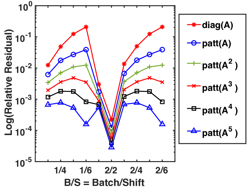
(a) SAM relative residual norm vs shift for Flow matrices, for all patterns without sparsification.

(b) SAM relative residual norm vs shift for Flow matrices, for all patterns with sparsification. “Sp Patt” indicates “Sparsified Pattern”.

Fig. 1: Relative SAM residual, $\frac{\|\mathbf{A}_{k}\mathbf{N}_{k}-\mathbf{A}_{0}\|_{F}}{\|\mathbf{A}_{0}\|_{F}}$, of the Flow matrices using a priori sparsity patterns for the SAM updates, $\mathbf{N}_{k}$, for batch/shift 1/3 through 2/6. An ILUTP preconditioner is computed for batch/shift 1/2. Details of these linear systems and the notation are provided in Sections 3 and 5.2.

Sparsity patterns derived from powers of the matrix, $\mathbf{A}$, are a standard choice. This choice is based on the decay of the elements in the matrix representing the discrete Green’s function [41, 68, 95] associated with the Laplace operator. While the denser sparsity patterns of higher powers of $\mathbf{A}$ may result in better maps, solving (8) becomes more costly. We can alleviate this cost by sparsifying the powers of $\mathbf{A}$. One possibility is to discard elements of $\mathbf{A}^{k}$ that are smaller in magnitude than a chosen threshold [41]. An alternative are sparsity patterns derived from the mesh on which the matrix is based. Using the underlying mesh for the topology optimization application, we experiment with sparsity patterns that are subsets of the sparsity pattern of the matrix, leading to maps that are much sparser than the system matrix.

We first analyze sparsity patterns defined by powers of the matrix, from $\mathbf{A}$ to $\mathbf{A}^{5}$, sparsifications of those, and the diagonal pattern. The sparsifications are obtained using a global threshold of $10^{-2}$. To further minimize cost, we first sparsify $\mathbf{A}$ using this global threshold, and then take powers of the logical matrix representing the nonzero pattern of this sparsified $\mathbf{A}$. We test these patterns for the Flow matrices [77, 78]. We study the relative residual norms of the resulting SAMs, the time to compute the map, the number of GMRES iterations and GMRES runtime, and the total solution time. GMRES(200) is used for this application. As the sparsity pattern of the map becomes denser, we expect the approximation in (8) to become more accurate, resulting in fewer GMRES iterations.

We consider eleven Flow matrices, $\mathbf{A}_{k}=s_{k}\mathbf{E}-\mathbf{A}$, and corresponding linear systems for a fixed right hand side $\mathbf{b}$ (see Section 5.2). The Iterative Rational Krylov Algorithm (IRKA) [63] computes optimal interpolation points, or shifts. Each iteration of IRKA generates a batch of new shifts until IRKA converges. We will refer to these matrices using the notation batch/shift (e.g., 1/2 is batch 1, shift 2). We consider shifts 2 through 6 and 1 through 6 of batches 1 and 2, respectively (see Table 16 in Section 5.2 for a list of all shifts).

We compute an ILUTP preconditioner, $\mathbf{P}_{0}$, for the first system in the sequence, $\mathbf{A}_{0}$, and we consider the powers of $\mathbf{A}_{0}$ to derive the denser patterns. For the Flow application, we compute and recycle the preconditioner for 1/2, not 1/1. For this first shift the matrix is quite ill-conditioned and not diagonally dominant, and this leads to a poor ILUTP preconditioner. So, we compute an ILUTP for this second matrix and recycle it for subsequent systems. We define the residual of the map and its relative residual norm as

$$\mathbf{R}_{k}=\mathbf{A}_{k}\mathbf{N}_{k}-\mathbf{A}_{0}\quad\mbox{and }\quad\frac{\|\mathbf{A}_{k}\mathbf{N}_{k}-\mathbf{A}_{0}\|_{F}}{\|\mathbf{A}_{0}\|_{F}}.$$

Figure 1 gives the relative residual norm for all shifts and all patterns, and Tables 1 and 2 give, for all patterns, GMRES iterations for selected shifts and (total) runtimes.

Batch/Shift	Diag	Patt $\mathbf{A}$	Patt $\mathbf{A}^{2}$	Patt $\mathbf{A}^{3}$	Patt $\mathbf{A}^{4}$	Patt $\mathbf{A}^{5}$
1/2	13	13	13	13	13	13
1/3	20	19	18	17	16	15
1/4	33	30	27	27	25	23
1/5	108	53	49	44	38	31
1/6	202	79	54	34	20	13
2/1	496	488	1620	(5001)	(5001)	(5001)
2/2-2/6	376	194	160	134	112	95
************ Totals ************
Total Iter	1235	863	1928	5257	5212	5178
SAM Time (s)	1.04	2.04	3.57	9.43	19.33	41.42
GMRES Time (s)	3.16	1.47	3.49	11.70	14.41	16.36
Total Time (s)	4.21	3.52	7.07	21.13	33.73	57.78
nnz($\mathbf{N}_{k}$)/n	1	6.97	18.94	37.02	61.39	92.36
********** Totals without 2/1 **********
Total Iter	739	375	308	256	211	177
SAM Time (s)	0.95	1.85	3.22	8.51	17.41	37.30
GMRES Time (s)	2.44	0.75	0.60	0.56	0.54	0.53
Total Time (s)	3.39	2.59	3.83	9.07	17.95	37.82

Table 1: GMRES iterations and total runtimes for selected shifts of the Flow matrices using a priori sparsity patterns for the SAM update. An ILUTP preconditioner is computed for the system 1/2, with SAM updates computed for all remaining shifts 1/3-2/6. “Patt” indicates “”Pattern of”. “SAM time” is the total amount of time spent computing all ten maps (but not including the time to compute the initial ILUTP). The initial ILUTP takes 0.8 s to compute. Totals are given for the entire sequence, as well as for the sequence omitting system 2/1. (5001) indicates GMRES did not converge in the maximum allowed iterations.

Batch/Shift	Sp Patt $\mathbf{A}$	Sp Patt $\mathbf{A}^{2}$	Sp Patt $\mathbf{A}^{3}$	Sp Patt $\mathbf{A}^{4}$	Sp Patt $\mathbf{A}^{5}$
1/2	13	13	13	13	13
1/3	19	18	17	16	15
1/4	30	27	27	25	23
1/5	53	50	45	40	34
1/6	81	62	48	39	35
2/1	(5001)	1437	(5001)	(5001)	(5001)
2/2-2/6	196	170	149	133	120
************** Totals**************
Total Iter	5380	1764	5287	5254	5228
SAM Time (s)	1.95	3.13	6.46	12.37	25.64
GMRES Time (s)	8.57	3.14	10.79	12.48	14.60
Total Time (s)	10.52	6.27	17.25	24.86	40.24
nnz($\mathbf{N}_{k}$)/n	5.30	13.64	26.26	43.36	65.39
************ Totals without 2/1 ************
Total Iter	379	327	286	253	227
SAM Time (s)	1.75	2.83	5.82	11.14	23.11
GMRES Time (s)	0.80	0.69	0.65	0.61	0.58
Total Time (s)	2.55	3.52	6.57	11.75	23.69

Table 2: GMRES iterations and total runtimes for selected shifts of the Flow matrices using a priori sparsified sparsity patterns. A global threshold of $10^{-2}$ is used to sparsify. An ILUTP preconditioner is computed for system 1/2, with SAM updates computed for all remaining shifts 1/3-2/6 “Sp Patt” indicates “Sparsified Pattern”. “SAM time” is the total amount of time spent computing all maps (but not including the time to compute the initial ILUTP). The initial ILUTP takes 0.8 s to compute. Totals are given for the entire sequence, as well as the sequence omitting system 2/1. (5001) indicates GMRES did not converge in the maximum allowed iterations.

The data show that for subsequent shifts of increasing magnitude, the relative residual norm grows and the recycled preconditioner $\mathbf{N}_{k}\mathbf{P}_{0}$ becomes less effective, resulting in more GMRES iterations as expected. Nevertheless, recycling preconditioners using SAMs keeps the iteration counts relatively low for most shifts; see Section 5.2 for more details and for comparison with the results listed here. The data also show that, as the relative residual norm decreases for denser patterns, the number of iterations decreases as well, with the exception of batch/shift 2/1, which corresponds to a very hard system. In Tables 1 and 2, we also show the cumulative results for both the entire sequence, as well as the sequence omitting batch/shift 2/1. In these tables, we specifically show iterations for batch/shift 1/2 through 2/1, and then aggregate numbers for batch/shift 2/2-2/6. For 2/2-2/6, the iterations for each shift (and the rate of growth of those iterations) are similar to those of 1/2-2/6.

However, for the sparsity patterns derived from higher powers of $\mathbf{A}_{0}$, the decrease in runtime from reduced GMRES iterations does not outweigh the increased costs of computing more expensive SAMs. For the Flow matrices, using the pattern of $\mathbf{A}_{0}$ comes out as the most efficient for total runtime (both with and without batch/shift 2/1), and we use this pattern for the experiments in Section 5.2. Though, if we omit batch/shift 2/1, the sparsified pattern of $\mathbf{A}_{0}$ leads to a slightly lower overall total runtime.

Next, we analyze sparsity patterns derived from the finite element mesh from which the matrices are derived, and we focus on subsets of the sparsity pattern of the system matrix that are much sparser than the matrix itself. This leads to maps that are cheap to compute compared with ILU-type preconditioners, which is particularly relevant for matrices that have many nonzeros per column. For this reason, we examine a sequence of matrices arising in topology optimization [98, 100] that result from discretization of the 3D linear elasticity equations on a $100\times 20\times 20$ trilinear (B8) element mesh, with three unknowns per node, $u$, $v$, and $w$, giving the displacements in the x-, y-, and z-direction. We order nodes and variables per node lexicographically. The size of these matrices is $n=132$ $300$, a typical column has up to 81 nonzeros, and the average number of nonzeros per column varies but is approximately $70$ (after the first few iterations). In the numerical results given in Section 5.1, we also consider a second, larger mesh for topology optimization.

To describe the stiffness matrix derived from the mesh, we consider a typical node $(i,j,k)$ that is not on the boundary. Let $s$, $s+1$, and $s+2$ be the column indices corresponding to the $u$, $v$, and $w$ variables, respectively, for node $(i,j,k)$. Then columns $s+3$, $s+4$, and $s+5$ correspond to the $u$, $v$, and $w$ variables, respectively, for node $(i+1,j,k)$, and columns $s-3$, $s-2$, and $s-1$ correspond to the $u$, $v$, and $w$ variables for node $(i-1,j,k)$. Column $s+300$ corresponds to the $u$ variable for node $(i,j+1,k)$, and $s+6300$ corresponds to the $u$ variable for node $(i,j,k+1)$. For the remainder of the stiffness matrix, we refer to Figure 2(a), which shows the column indices, $s+m$, corresponding to the $u$ variables of nodes in elements that contain node $(i,j,k)$. The column indices for the $v$ and $w$ variables at those nodes are given by $s+m+1$ and $s+m+2$, respectively, for each $m$.

With 27 nodes, each with three displacements, there are numerous choices in sub-patterns of the matrix sparsity pattern that can be made depending on user preference. A user may include certain displacements and omit others, dictating how many and which nonzeros will be included in the sparsity pattern. We evaluate five of such possible patterns, Patt-0 to Patt-4. For each, we choose a selection of mesh nodes relative to $(i,j,k)$ and displacements associated with those nodes. We stress that each of these patterns (and any of the other resulting patterns from choosing a different subset of displacements) are much sparser than the stiffness matrix itself.

To define Patt-0 for the $u$ column of the node $(i,j,k)$, corresponding to column $s$, we combine its index with the index for the $u$ variable at the nodes marked by ‘$\times$’ in Figure 2(b). The resulting sparsity pattern contains, for column $s$, the ordered pairs $(s,s)$, $(s\pm 3,s)$, $(s\pm 300,s)$, and $(s\pm 6300,s)$. For the $v$ and $w$ columns, we use the same pattern, but with $s$ indicating the $v$, respectively, $w$ column for node $(i,j,k)$. On boundaries, this pattern is adjusted to take the boundary and boundary conditions into account. This will also be done for Patt-1 discussed below.

Patt-1 was obtained by experimenting with minor variations of Patt-0. This sparsity pattern contains, for column $s$, the ordered pairs $(s,s)$, $(s\pm 1,s)$, $(s\pm 300,s)$, and $(s\pm 6000,s)$. For the $v$ and $w$ columns, we use the same pattern, but with $s$ indicating the $v$, respectively, $w$ column for node $(i,j,k)$. Patterns Patt-2, Patt-3, and Patt-4 include more column indices from the original sparsity pattern of the matrix based on the finite element mesh described above. All patterns, Patt-0–Patt-4, contain substantially fewer nonzeros than the stiffness matrix. Table 3 shows the numbers of nonzeros in the sparsity patterns with timing and iterations results.

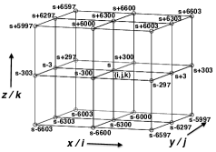
(a) The $8$ elements containing node $(i,j,k)$ and the column indices, $s+m$, in the stiffness matrix that correspond to the $u$ variables of their nodes, where $s$ is the column index corresponding to the $u$ variable for node $(i,j,k)$.

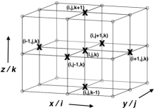
(b) Mesh nodes involved in the sparsity pattern Patt-0. The details are given in the text.

Fig. 2:

To evaluate the effectiveness of these patterns, we compute an ILUTP preconditioner for the matrix at optimization step 100, and compute SAMs for the matrices at steps 105, 110, 115, 120, 125, and 130. We solve the preconditioned systems using full GMRES. The results are shown in Table 3. While these maps have substantially fewer nonzeros than the matrices themselves, recycling the initial preconditioner using these SAMs keeps the GMRES iterations low. When computing the SAM with either Patt-0 or Patt-1, each map takes less than three seconds to compute. Including more nonzeros from the sparsity pattern of the stiffness matrix (Patt-2–Patt-4), decreases the total number of GMRES iterations a bit further; however, there is a substantial increase in the time to compute the maps. Both times and iteration counts are comparable between Patt-0 and Patt-1 as shown in Table 3, though the latter is slightly faster across the longer sequence of topology optimization matrices considered in Section 5.1. So, we show results using Patt-1 for those experiments. In particular, we demonstrate the effectiveness of recycling preconditioners using SAMs in detail in Section 5, providing comparisons with recomputing preconditioners and reusing preconditioners for several applications.

Optimization	Patt-0	Patt-1	Patt-2	Patt-3	Patt-4
Step	Iter	Iter	Iter	Iter	Iter
100	166	166	166	166	166
105	173	173	173	170	169
110	184	184	183	177	176
115	195	196	194	184	183
120	208	208	205	190	189
125	216	220	213	194	193
130	228	226	222	197	197
Total Iter	1370	1373	1356	1278	1273
SAM Time (s)	14.96	15.10	45.47	91.52	97.23
GMRES Time (s)	97.21	98.49	98.19	95.03	94.96
Total Time (s)	234.57	236.00	266.06	308.96	314.61
nnz($\mathbf{N}_{k}$)/n	5.47	5.33	9.46	29.07	33.67

Table 3: GMRES iterations and total runtimes for matrices from selected steps of the topology optimization application using a priori mesh-based sparsity patterns. “SAM time” is the total amount of time spent computing all maps (but not including the time to compute the initial ILUTP). The initial ILUTP takes $122.41$s to compute.

4 Implementation

We have developed efficient implementations for computing SAMs and ILUTP preconditioners as MATLAB^®  m-files to make useful runtime comparisons between recycling a preconditioner and computing a new one. We use a MATLAB^® implementation of the AMG preconditioner developed as part of work done in [67]. We also refer the reader to [84, 85, 92, 94, 93] [97, Appendix A: An Introduction to Algebraic Multigrid, K. Stüben].

First, we describe an efficient implementation for computing SAMs. To efficiently compute the SAM updates, the solution of (8) should be implemented in sparse-sparse fashion. For most problems, the nonzero pattern of the matrices does not change, and we preprocess the sparsity pattern for the maps to set up data structures for the small least squares problems just once; see Algorithm 1. Since we store $\mathbf{A}_{k}$ as a MATLAB^®  sparse matrix, access to columns is cheap.

Given a pattern, $S$, $s_{\ell}=\{i\,|\,(i,\ell)\in S\}$, the set of indices of potential nonzeros in $\mathbf{n}_{\ell}$, column $\ell$ of $\mathbf{N}_{k}$. To compute $\mathbf{n}_{\ell}$, we only need the $m$ columns $\mathbf{a}_{j}$ of $\mathbf{A}_{k}$ such that $j\in s_{\ell}$, and as these columns are sparse we need only consider rows $i$ such that $a_{i,j}\neq 0$ for some $j\in s_{\ell}$. Let $r_{\ell}$ be the set of relevant row indices. Then the least squares problem for $\mathbf{n}_{\ell}$ is defined as

$$\mathbf{n}_{\ell}(s_{\ell}) = \arg\min_{\widetilde{\mathbf{n}}\in\mathbb{C}^{m}}\|\mathbf{A}_{k}(r_{\ell},s_{\ell})\widetilde{\mathbf{n}}-\mathbf{A}_{0}(r_{\ell},\ell)\|_{2},$$

where $\mathbf{A}_{k}(r_{\ell},s_{\ell})$ is the submatrix of $\mathbf{A}_{k}$ indexed by $r_{\ell}\times s_{\ell}$, and $\mathbf{A}_{0}(r_{\ell},\ell)$ is the corresponding part of the $\ell$th column of $\mathbf{A}_{0}$. Note that if $(a_{0})_{i,\ell}\neq 0$ but $a_{i,j}=0$ for all $j\in s_{\ell}$, row $i$ is irrelevant for computing $\mathbf{n}_{\ell}$ since $\mathbf{e}_{i}\perp\mathrm{Span}(\{\mathbf{a}_{j}\,|\,j\in s_{\ell}\})$. However, if we wish to compute, in addition to $\mathbf{N}_{k}$, the residual $\mathbf{R}_{k}=\mathbf{A}_{k}\mathbf{N}_{k}-\mathbf{A}_{0}$ or its norm on Line 7 of Algorithm 2, we need to include such rows as well. If the matrices $\mathbf{A}_{k}$ and $\mathbf{A}_{0}$ have the same sparsity pattern and the pattern of $\mathbf{N}_{k}$ includes at least the diagonal, this is not an issue. So, the size of each least squares problem depends only on the chosen sparsity pattern of $\mathbf{N}$ and the sparsity pattern of $\mathbf{A}_{k}$, not on the matrix size. So the least squares problems are small, independent of $n$, and most are about the same size. For example, for the Flow application discussed in Section 5.2, the maximum size of the least squares problems to compute the SAM updates is $20\times 7$, independent of $n=9~{}669$.

Finally, to ensure the map is computed and then stored as efficiently as possible, in Lines 3-11 of Algorithm 2, we compute $\mathbf{N}$ in coordinate format (COO). After the entire map has been computed, we convert this temporary data structure into a MATLAB^®  sparse matrix using the command sparse in Line 12.

Algorithm 1 Preprocessing for Computing Sparse Approximate Maps

1:Given sparsity pattern $S$ and matrix $\mathbf{A}$

2:$maxSk=0$; $maxRk=0$; { initialize max num of columns, max num of rows }

3:for $k=1:n$ do { for each column do }

4:     $s_{k}=\{i\,|\,(i,k)\in S\}$ { get indices; typically defined in advance }

5:     $r_{k}=\emptyset$ { Initialize set of rows for $k$th LS problem }

6:     for all $j\in s_{k}$ do

7:         $t=\texttt{find}(\mathbf{a}_{j})$ { find indices of nonzeros in column $\mathbf{a}_{j}$ }

8:         $r_{k}=r_{k}\cup t$

9:     end for

10:     $nnz_{k}=\#(s_{k})$ { #() gives number of elements in a set } if $nnz_{k}>maxSk$ then $maxSk=nnz_{k}$ end if if $\#(r_{k})>maxRk$ then $maxRk=\#(r_{k})$ end if

11:end for

12:Allocate $maxRk\times maxSk$ array for storing the LS matrices, $maxRk$ vector for storing the right hand side, and $maxSk$ vector for storing the solution.

Algorithm 2 Computing $\mathbf{N}=\arg\min_{\widetilde{\mathbf{N}}\in{\mathcal{S}}}\|\mathbf{A}\widetilde{\mathbf{N}}-\widehat{\mathbf{A}}\|_{F}$

1:$cnt=0$ { counts number of nonzeros in preconditioner }

2:(Preallocate space for $\mathbf{A}_{\mathrm{tmp}}$)

3:for $k=1:n$ do

4:     $\mathbf{A}_{\mathrm{tmp}}=\mathbf{A}(r_{k},s_{k})$ { get submatrix indexed by $r_{k}$ and $s_{k}$ for LS problem }

5:     $\mathbf{f}=\widehat{\mathbf{A}}(r_{k},k)$ { get rhs for LS problem }

6:     Solve LS $\mathbf{A}_{\textrm{tmp}}\mathbf{z}=\mathbf{f}$

7:     (possibly save residual, norm of residual, etc.)

8:     $rowN[cnt+1:cnt+nnz_{k}]=s_{k}$ { assign indices in order of row ind. in $s_{k}$ }

9:     $colN[cnt+1:cnt+nnz_{k}]=k$

10:     $valN[cnt+1:cnt+nnz_{k}]=\mathbf{z}$

11:end for

12:$\mathbf{N}=$ sparse$(rowN,colN,valN)$ { convert into sparse matrix }

Our implementation of ILUTP closely follows [86, 87]. To make the implementation efficient in MATLAB^®, we made the following main changes. (1) We transpose $\mathbf{A}$, in MATLAB^®  sparse matrix storage, to access the rows efficiently. (2) Where possible, we use MATLAB^®  routines, such as find, sort, sparse, and min. (3) Where possible, we have vectorized loops. (4) We use sparse to build $\mathbf{L}$ and $\mathbf{U}$ efficiently, and we use tril and triu to ensure MATLAB^®  recognizes and uses the $\mathbf{L}$ and $\mathbf{U}$ factors as triangular matrices. The m-file is available from [58].

5 Numerical Experiments

We analyze the effectiveness of reusing, recomputing, and recycling preconditioners for several applications. All systems are solved using preconditioned GMRES. We compare the results of computing a new ILUTP or AMG preconditioner for each matrix or selected matrices, reusing the initial $\mathbf{P}_{0}$ for all systems, updating $\mathbf{P}_{0}$ with a new SAM update for all systems, and updating $\mathbf{P}_{0}$ with a SAM update only at selected systems in the sequence, combined with computing a new $\mathbf{P}_{0}$ at selected systems. Computing a new preconditioner for every matrix is always the most expensive in runtime, but it provides a useful benchmark in terms of the number of iterations. Computing a SAM update only at selected systems (for a long sequence, combined with recomputing the preconditioner at selected systems) is usually the winner in runtime. We report runtimes for computing preconditioners and SAMs, the number of iterations and runtime to solve each system, and total runtime and number of iterations for the whole sequence. Our focus is total runtime.

We tested several indicators for computing a new SAM update or new preconditioner. A simple and effective strategy is to compute a new SAM or preconditioner based on the estimated time for this computation and the (relative) increase in the solution time for a system or the number of iterations. For the smaller the topology optimization problem, we give results for recomputing based on a percent increase in iterations.

5.1 Topology Optimization

This test problem leads to a long sequence of linear systems, where the matrix has a relatively large number of nonzeros per row. As a result, this problem is particularly useful to demonstrate effective SAMs that are much sparser than the matrix itself.

Topology optimization is a structural optimization method that optimizes the material distribution inside a given domain [21, 76, 81, 91, 100]. The method computes a design by determining which points of space should be material and which points should be void (i.e. no material), combining finite element approximation, linear solvers (for linear partial differential equations), and optimization. In this case, we minimize the compliance (see below) subject to a volume constraint. We specify the problem mathematically as follows.

$$\min_{{\bf\rho},\mathbf{u}}\> c({\bf\rho},\mathbf{u})=\mathbf{u}^{T}\mathbf{A}({\bf\rho})\mathbf{u}$$

s.t. $$\mathbf{A}({\bf\rho})\mathbf{u}=\mathbf{f}$$

$$0<\rho_{0}\leq\rho_{e}\leq 1\qquad e=1,2,\cdots,n_{e}$$

$$\int_{\Omega}\rho\,\mathrm{d}\Omega\leq V,$$

where $c$ is the compliance, $\mathbf{A}({\bf\rho})$ is the stiffness matrix as a function of the density distribution ${\bf\rho}$, $\mathbf{u}$ and $\mathbf{f}$ are the displacement vector and load vector, $\rho_{0}$ is a chosen, small, positive lower bound for the density to avoid singularity of the stiffness matrix, and $V$ is the total volume in use. The Solid Isotropic Material with Penalization (SIMP) method [18, 20] uses one design variable to represent the density in each element.

The structure of the matrices is detailed in Section 3. We consider matrices that result from discretizing the 3D linear elasticity equations for variable density on a trilinear (B8) finite element mesh. We examine two such meshes with (1) $100\times 20\times 20$ elements, and (2) $150\times 30\times 30$ elements, with three unknowns per node, $u$, $v$, and $w$, giving the displacements in the x-, y-, and z-directions resulting in matrices of sizes (1) $n=132$ $300$, and (2) $n=432$ $450$. (see [98, 100] for details). We refer to these respectively as the “small” and “large” topology optimization matrices. For both, we take a representative sequence from an optimization that typically takes hundreds, but possibly up to 1000, optimization steps before reaching the optimal design. We demonstrate the effects of several strategies for reusing, recycling, and recomputing the preconditioner. We use the ILUTP preconditioner for the small matrices and the AMG preconditioner for the large matrices. Results are provided in Tables 5-9.

For the large matrices, we show that in the case of an expensive preconditioner resulting in fast GMRES convergence, we can preserve this good convergence with SAM updates. We use a path cover adaptive algebraic multigrid [67] for the preconditioner. The grid and operator complexities are 1.166 and 1.863, respectively. In particular, both are less than 2.0. The computation of this preconditioner takes about 16.5 minutes, whereas the SAM updates take less than five seconds, with five additional seconds for preprocessing at the first update. We use full GMRES with maximum iterations set to 400 and the zero initial guess.

Table 5 shows the results when we reuse the initial AMG preconditioner. In this case, the GMRES iterations grow quickly and reach the maximum allowed twice. At that point, we compute a new preconditioner and reuse it for subsequent systems. So, we recompute the preconditioner halfway through the sequence and would do this again at optimization step 70. Total computation time is nearly two hours. Apparently, modest changes in material distribution may already make the coarse grid correction in the AMG preconditioner substantially less effective.

Table 5 shows the results when we update the initial AMG preconditioner using SAMs at every step. We use Patt-1, described in Section 3, which has seven nonzeros in a typical column compared with up to 81 nonzeros in a typical column of the stiffness matrix. As a single GMRES iteration takes about two seconds (in both tests) due to the ILU-smoothing in the AMG preconditioner, preserving a low number of iterations is important. Recycling the initial preconditioner using SAM updates achieves this goal, with the number of iterations growing slowly from 35 to 101, avoiding recomputations of the preconditioner. The total computation time when recycling the AMG preconditioner using SAMs is reduced to less than 38 minutes.

Mats	Prec	GMRES	Iter
	(s)	(s)
60	994.52	80.34	35
61	0	127.03	58
62	0	222.88	99
63	0	416.09	171
64	0	741.18	299
65	0	1026.75	400
66	1002.24	83.57	37
67	0	168.36	77
68	0	623.67	259
69	0	1026.96	400
Total	6526.20		1835

Table 4: Runtimes and iterations for the large top opt systems, when reusing the AMG preconditioner for each system after the first. When max iterations (400) is reached, we recompute the AMG preconditioner for the next system and reuse this for subsequent systems.

Mats	Prec	GMRES	Iter
	(s)	(s)
60	994.52	80.34	35
61	10.52	81.92	38
62	4.97	88.08	41
63	4.89	94.31	44
64	4.75	101.35	47
65	4.80	112.10	52
66	4.89	126.10	58
67	4.92	147.39	68
68	4.95	177.88	81
69	4.93	221.85	101
Total	2275.47		565

Table 5: Runtimes and iterations for the large top opt systems, when computing the AMG preconditioner for the first system and a SAM update for each system after the first. SAMs use the sparsity pattern Patt-1.

For the small top opt matrices, computing the ILUTP preconditioner takes about two minutes. Fill in for ILUTP is set to 250 and the drop tolerance is $10^{-3}$. We use Patt-1 for the SAMs, as it gives slightly faster runtimes then Patt-0 for the sequence of systems considered here. Computing a SAM update takes a bit over two seconds. We use full GMRES with maximum number of iterations set to $1000$. When computing an ILUTP preconditioner for top opt matrices, diagonal scaling is essential to mitigate the huge ratio in local stiffness [99]. This scaling varies with each matrix and combined with pivoting complicates using the previous solution as initial guess, so we use the zero initial guess. Table 7 provides the results for reusing the initial preconditioner for all systems. Results for computing a new preconditioner for every system are not shown, given the high cost of computing the ILUTP. Computing the SAM update for every matrix after the first reduces iterations substantially, but is still too expensive in runtime. Therefore, we compute a SAM update for each tenth system and reuse the recycled preconditioner until the next update. Results are provided in Table 7.

Mats	Prec	GMRES	Iter
	(s)	(s)
40-49	120.85	134.98	1909
50-59	0	202.42	2667
60-69	0	272.05	3353
70-79	0	331.72	3880
80-89	0	396.47	4405
90-99	0	892.64	7405
100-109	0	1375.30	(9779)**
110-119	0	1430.16	(10010)*
120-129	0	1432.25	(10010)*
130-139	0	1436.56	(10010)*
140-149	0	1429.65	(10010)*
150-166	0	2454.73	(10010)*
Totals	11909.79		90455

Table 6: Runtimes and iterations for the small top opt systems with the initial ILUTP reused for all systems. Results are given in groups of ten except for (150-166). **For only one system converge reached within max iterations. *Convergence not reached for any system within max iterations.

Mats	Prec	GMRES	Iter	Gain	Gain
	(s)	(s)		GMRES (s)	Iter
40-49	120.85	134.98	1909	0	0
50-59	2.41	189.72	2495	–12.71	–172
50-69	2.19	241.57	3012	–30.48	–341
70-79	2.15	283.75	3396	–47.97	–484
80-89	2.13	333.22	3823	–63.25	–582
90-99	2.14	361.81	4067	–530.83	–3338
100-109	2.14	404.84	4414	–970.46	–5365
110-119	2.14	476.00	4799	–954.16	–5211
210-129	2.29	446.45	4689	–985.80	–5321
130-139	2.15	465.68	4844	–970.88	–5166
140-149	2.18	535.47	5324	–894.18	–4686
150-166	4.30	1689.75	(13187)*	–903.72	–3830
Totals	5710.32		55959	–6225.71	–34496

Table 7: Runtimes and iterations for the small top opt systems with the initial ILUTP recycled with a SAM update for every tenth system, using Patt-1. Results are given in groups of ten except for (150-166). “Gain” indicates the decrease in GMRES time and iterations compared with reusing the initial ILUTP. There are two SAM updates in (150-160). *For one matrix convergence not reached within max iterations.

We can improve runtimes by recomputing the ILUTP preconditioner and the SAMs based on increases in iterations. We refer to this strategy as the “dynamic strategy”. Considering only the ILUTP preconditioner, we recompute the preconditioner when the number of iterations at an optimization step increases by 50% over those from the latest ILUTP computation. Table 9 shows the results. In addition, we can compute a SAM update when the number of iterations at an optimization step increases by 20% over those from the latest ILUTP computation. We only compute one SAM update between ILUTP computations. The results are given in Table 9.

Mats	Prec	GMRES	Iter	ILUTP
	(s)	(s)		at Step
40-53	120.85	210.85	2891	40
54-74	120.92	320.93	4402	54
75-98	123.24	358.48	4921	75
99-132	120.26	524.04	7181	99
133-162	121.42	433.29	5827	133
162-166	121.21	46.49	667	162
Totals	2621.90		26055	($\times 6$)

Table 8: Runtimes and iterations for the small top opt matrices with the dynamic strategy for ILUTP only. Each group of systems starts with a new ILUTP, as indicated in the last column.

Mats	Prec	GMRES	Iter	ILUTP	SAM
	(s)	(s)		at Step	at Step
40-54	123.29	223.513	3057	40	47
55-77	122.52	358.62	4735	55	66
78-103	122.65	391.04	5297	78	90
104-144	122.31	610.46	8305	104	122
145-166	122.95	295.21	4083	145	160
Totals	2492.50		25477	($\times 5$)	($\times 5$)

Table 9: Runtimes and iterations for the small top opt matrices with the dynamic strategy for both ILUTP and SAM updates with Patt-1. Each group of systems starts with a new ILUTP, and includes one SAM update, as indicated in the last two columns.

The dynamic strategy for both ILUTP computation and SAM update reduces the total number of GMRES iterations (by 578 iterations), the overall runtime (by 129 seconds), and the number of ILUTP computations (by 1) compared with the dynamic strategy for the ILUTP preconditioner only. Over the full sequence of optimization steps, these numbers increase proportionally.

5.2 Interpolatory Model Reduction

Our next set of linear systems arises in the Iterative Rational Krylov Algorithm (IRKA) [63, 8] for computing $H_{2}$-optimal interpolatory reduced order models [8]. Model reduction aims to replace a high-dimensional linear dynamical system (here single-input/single-output)

$$\mathbf{E}\dot{\mathbf{x}}(t)+\mathbf{A}\mathbf{x}(t)=\mathbf{b}u(t),\hskip 11.38109pty(t)=\mathbf{c}^{T}\mathbf{x}(t),$$ (19)

where $\mathbf{E},\mathbf{A}\in\mathbb{R}^{n\times n}$, $\mathbf{b},\mathbf{c}\in\mathbb{R}^{n}$, input and output $u(t),y(t)\in\mathbb{R}$, and state vector $\mathbf{x}(t)\in\mathbb{R}^{n}$, and $n$ is very large, by a much lower dimensional dynamical system

$$\mathbf{E}_{r}\dot{\mathbf{x}}_{r}(t)+\mathbf{A}_{r}\mathbf{x}_{r}(t)=\mathbf{b}_{r}u(t),\hskip 11.38109pty_{r}(t)=\mathbf{c}_{r}^{T}\mathbf{x}_{r}(t),$$ (20)

where $\mathbf{E}_{r},\mathbf{A}_{r}\in\mathbb{R}^{r\times r}$, $\mathbf{b}_{r},\mathbf{c}_{r}\in\mathbb{R}^{r}$, and $r\ll n$, such that $y_{r}(t)\approx y(t)$ in an appropriate norm for a wide range of input selections $u(t)$. Here, for brevity, we consider single-input/single-output dynamical systems, i.e., $u(t)$ and $y(t)$ are scalar valued functions. Discussion similarly extends to the multi-input/multi-output case. Dynamical systems with large state-space dimension $n$ appear in many applications, ranging from nonlinear parameter inversion to optimal control to circuit design. The repeated simulation of these large systems may be infeasible, but model reduction allows us to do sufficiently accurate simulations with a much smaller system.

The reduced model quantities in (20) are obtained by construction of the matrices $\mathbf{V}_{r},\mathbf{W}_{r}\in\mathbb{R}^{n\times r}$ (the model reduction bases) and a Petrov-Galerkin projection

$$\mathbf{A}_{r}=\mathbf{W}_{r}^{T}\mathbf{A}\mathbf{V}_{r},\hskip 11.38109pt\mathbf{E}_{r}=\mathbf{W}_{r}^{T}\mathbf{E}\mathbf{V}_{r},\hskip 11.38109pt\mathbf{b}_{r}=\mathbf{W}_{r}^{T}\mathbf{b},\hskip 11.38109pt\mathbf{c}_{r}=\mathbf{V}_{r}^{T}\mathbf{c}.$$ (21)

Model reduction approaches differ in their choices of $\mathbf{V}_{r}$ and $\mathbf{W}_{r}$ [6, 8, 13, 22, 23, 79, 64]. In interpolatory model reduction, $\mathbf{V}_{r}$ and $\mathbf{W}_{r}$ are constructed so that the reduced model transfer function $H_{r}(s)=\mathbf{c}_{r}^{T}(s\mathbf{E}_{r}-\mathbf{A}_{r})^{-1}\mathbf{b}_{r}$ is a rational interpolant of the full model transfer function $H(s)=\mathbf{c}^{T}(s\mathbf{E}-\mathbf{A})^{-1}\mathbf{b}$. In this case, we focus on the case that $H_{r}(s)$ is a Hermite interpolant to $H(s)$ as this is required for optimality [63, 8]. Therefore, the goal is to construct $\mathbf{V}_{r}$ and $\mathbf{W}_{r}$ such that $H_{r}(s_{j})=H(s_{j})$ and $H^{\prime}_{r}(s_{j})=H^{\prime}(s_{j})$ for some given set of points $s_{1},\ldots,s_{r}$. Constructing $\mathbf{V}_{r}$ and $\mathbf{W}_{r}$ as

$$\mathbf{V}_{r} =[(s_{1}\mathbf{E}-\mathbf{A})^{-1}\mathbf{b},\dots,(s_{r}\mathbf{E}-\mathbf{A})^{-1}\mathbf{b}],$$ (22)

$$\mathbf{W}_{r} =[(s_{1}\mathbf{E}^{T}-\mathbf{A}^{T})^{-1}\mathbf{c},\dots,(s_{r}\mathbf{E}^{T}-\mathbf{A}^{T})^{-1}\mathbf{c}],$$ (23)

achieves this; see [7, 8] for more details. IRKA [63] finds the optimal interpolation points by alternatingly computing (22)–(23) for a given set of interpolation points $\{s_{j}\}$ and computing a new set $\{s_{j}\}$ given $\mathbf{V}_{r}$ and $\mathbf{W}_{r}$; for details and some variants of IRKA, see [63, 8, 14, 65, 102, 37, 101]. Since IRKA may take many iterations to converge to the final set of interpolation points $\{s_{j}\}$, many shifted systems must be solved in computing (22) and (23). Each set of shifts for an IRKA iteration is called a batch.

Efficient solution of (22)–(23) is an important research topic. In [15], inexact solves within a Petrov-Galerkin framework are used. In [5], the recycling BiCG algorithm is proposed for model reduction, which is extended to recycling BiCGSTAB for parametric model reduction in [3]. Further discussion of recycling Krylov subspace methods for model reduction applications can be found in [53, 54].

We give results for one set of matrices, Flow, from [78]. These matrices arise in a simulation of the heat exchange between a solid body and a fluid flow, and background on this benchmark problem can be found in [78]. Rather than using computational fluid dynamics, which is quite expensive, a flow region with a given velocity profile is used [77]. However, this requires a much larger number of elements, and model reduction is used to make the simulation efficient [77]. For more information see [75, 77, 78, 83]. The matrices $\mathbf{A},\mathbf{E}\in\mathbb{R}^{n\times n}$ are sparse with $n=9~{}669$. Although $\mathbf{A}$ is not symmetric, it turns out that the shifts remain real for the three steps of IRKA used here. We use three batches of six shifts, which are real and range from $O(1)$ to $O(10^{4})$. The shifts for the Flow matrices are provided in Table 16.

We use GMRES(200) for this application and set the maximum number of iterations to 5000. Fill in for ILUTP is 56 and the drop tolerance is $10^{-3}$. The pattern of $\mathbf{A}_{0}$ is used for the SAM updates. Results are given in Tables 16–16.

An interesting case arises here. The number of iterations for the first preconditioned system, $\mathbf{A}_{0}\mathbf{P}_{0}$, is very high. For this first shift, the matrix is ill-conditioned and not diagonally dominant, and this leads to a poor ILUTP preconditioner. It makes no sense to reuse or recycle this preconditioner. As an alternative, we compute a new preconditioner, $\mathbf{P}_{1}$, for the second system. As this preconditioned system results in fast convergence, we recycle $\mathbf{P}_{1}$ with SAMs for each subsequent system (see Table 16) and at select systems (see Table 16). This leads to much better iteration counts and lower runtimes. When computing SAM updates for select shifts, as shown in Table 16, for the other shifts we reuse $\mathbf{P}_{1}$, not the SAM updated preconditioner from a previous step. As IRKA converges, the shifts from one batch to the next do not change very much. If the initial preconditioner works well for certain shifts in one batch, we can reuse it for the corresponding shifts in subsequent batches (see Table 16). For comparison we also provide results with $\mathbf{P}_{1}$ reused for all subsequent systems, leading to sightly longer runtimes than using the SAMs (see Table 16).

As poor clustering of eigenvalues tends to lead to slow GMRES convergence, we compare the spectra of the preconditioned systems for two shifts. Figure 3 shows the spectrum of the initial preconditioned system, while Figures 4 and 5 show the spectra of preconditioned systems 1/5 and 1/6, respectively, when recomputing, recycling, and reusing the preconditioner computed for system 1/2. The figures show that the SAMs improve the eigenvalue clustering substantially, in particular along the real axis. At these shifts, SAMs result in much lower iterations compared with reusing the preconditioner (see Tables 16 and 16).

Shift	Batch 1	Batch 2	Batch 3
1	1.4091	1.4115	1.4116
2	28.123	30.121	30.146
3	150.70	163.43	163.58
4	669.26	691.84	692.12
5	3536.7	3565.9	3566.2
6	17329	17353	17353

Table 10: Shifts for the Flow Matrices.
For subsequent tables, B/S = Batch/Shift Number.

B/S	Prec	GMRES	Iter
	(s)	(s)
1/1	0.80	2.64	1941
1/2	0.73	0.03	13
1/3	0.70	0.02	11
1/4	0.67	0.02	10
1/5	0.62	0.02	7
1/6	0.55	0.02	7
2/1	0.71	0.60	455
2/2	0.70	0.03	13
2/3	0.70	0.03	11
2/4	0.70	0.03	11
2/5	0.62	0.02	7
2/6	0.55	0.02	7
3/1	0.71	5.66	4231
3/2	0.69	0.03	13
3/3	0.73	0.02	11
3/4	0.68	0.02	10
3/5	0.62	0.02	7
3/6	0.56	0.02	7
Total	21.28		6771

Table 11: Runtimes and iterations for the Flow matrices with ILUTP recomputed for each shift.

B/S	Prec	GMRES	Iter
	(s)	(s)
1/1	0.80	2.64	1941
1/2	0	0.02	18
1/3	0	0.03	26
1/4	0	0.59	206
1/5	0	0.59	211
1/6	0	0.62	232
2/1	0	0.02	15
2/2	0	0.02	18
2/3	0	0.05	41
2/4	0	0.60	207
2/5	0	0.62	210
2/6	0	0.78	231
3/1	0	4.00	3007
3/2	0	0.03	18
3/3	0	0.05	40
3/4	0	0.61	206
3/5	0	0.63	209
3/6	0	0.71	227
Total	13.41		7063

Table 12: Runtimes and iterations for the Flow matrices with ILUTP computed for the first shift and reused for each remaining shift.

B/S	Prec	GMRES	Iter
	(s)	(s)
1/1	0.80	2.64	1941
1/2	0.23	0.03	18
1/3	0.20	0.04	24
1/4	0.20	0.05	30
1/5	0.19	0.19	99
1/6	0.19	0.14	83
2/1	0.19	0.37	275
2/2	0.20	0.03	18
2/3	0.19	0.03	24
2/4	0.19	0.25	124
2/5	0.19	0.62	207
2/6	0.20	0.36	155
3/1	0.19	6.85	5001
3/2	0.19	0.03	18
3/3	0.19	0.03	24
3/4	0.19	0.25	124
3/5	0.19	0.19	99
3/6	0.19	0.57	196
Total	16.93		8619

Table 13: Runtimes and iterations for the Flow matrices with ILUTP computed for the first system and SAM updates computed for all other shifts.

B/S	Prec	GMRES	Iter
	(s)	(s)
1/1	0.80	2.64	1941
1/2	0.73	0.03	13
1/3	0.20	0.03	19
1/4	0.20	0.05	30
1/5	0.20	0.10	53
1/6	0.20	0.18	79
2/1	0.20	0.72	488
2/2	0.20	0.02	12
2/3	0.20	0.03	20
2/4	0.21	0.05	30
2/5	0.21	0.10	53
2/6	0.19	0.18	79
3/1	0.20	0.56	382
3/2	0.21	0.02	12
3/3	0.20	0.03	20
3/4	0.20	0.05	30
3/5	0.20	0.10	53
3/6	0.20	0.18	79
Total	9.83		3393

Table 14: Runtimes and iterations for the Flow matrices with ILUTP computed for the first two systems and SAM updates computed for all other shifts.

B/S	Prec	GMRES	Iter
	(s)	(s)
1/1	0.80	2.64	1941
1/2	0.73	0.03	13
1/3	0	0.03	21
1/4	0	0.11	60
1/5	0	0.84	202
1/6	0	0.89	215
2/1	0	0.12	86
2/2	0	0.02	12
2/3	0	0.03	21
2/4	0	0.06	37
2/5	0	0.97	202
2/6	0	0.89	215
3/1	0	0.69	486
3/2	0	0.02	12
3/3	0	0.03	22
3/4	0	0.06	36
3/5	0	0.96	202
3/6	0	1.01	215
Total	10.90		3998

Table 15: Runtimes and iterations for the Flow matrices with ILUTP computed for the first two systems, and $\mathbf{P}_{1}$ reused for all remaining shifts.

B/S	Prec	GMRES	Iter
	(s)	(s)
1/1	0.80	2.64	1941
1/2	0.73	0.03	13
1/3	0	0.03	21
1/4	0	0.11	60
1/5	0.20	0.10	53
1/6	0.20	0.19	79
2/1	0	0.12	86
2/2	0	0.02	12
2/3	0	0.03	21
2/4	0	0.06	37
2/5	0.21	0.10	53
2/6	0.20	0.18	79
3/1	0	0.68	486
3/2	0	0.02	12
3/3	0	0.03	22
3/4	0	0.06	36
3/5	0.21	0.10	53
3/6	0.19	0.18	79
Total	7.44		3143

Table 16: Timings for Flow matrices with ILUTP computed for the first two systems and SAM updates computed for selected shifts.

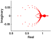
Fig. 3: Eigenvalues of preconditioned system 1/2, $\mathbf{A}_{1}\mathbf{P}_{1}$, with the preconditioner recomputed.

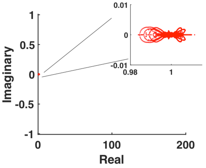
(a)

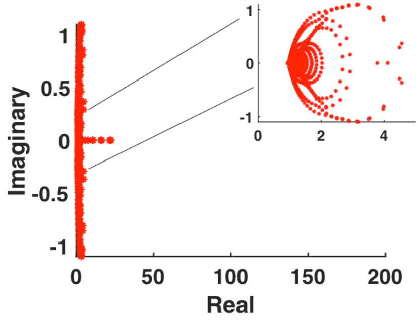
(b)

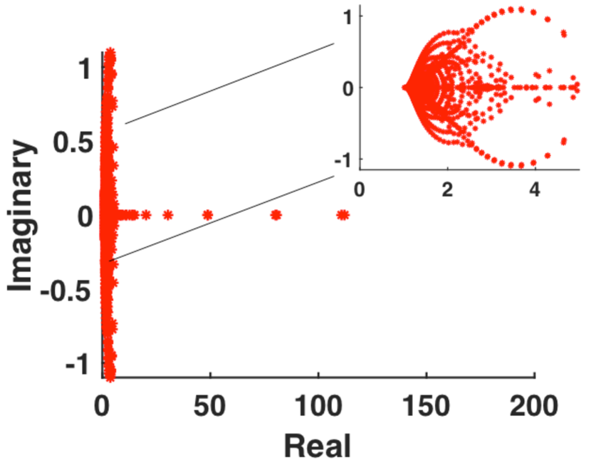
(c)

Fig. 4: Eigenvalues of preconditioned system 1/5 with (a) $\mathbf{P}_{4}$ recomputed, (b) $\mathbf{P}_{4}=\mathbf{N}_{4}\mathbf{P}_{1}$ (recycled), and (c) $\mathbf{P}_{1}$ reused. Note the different scale along the real axis compared with Figure 3 and 5.

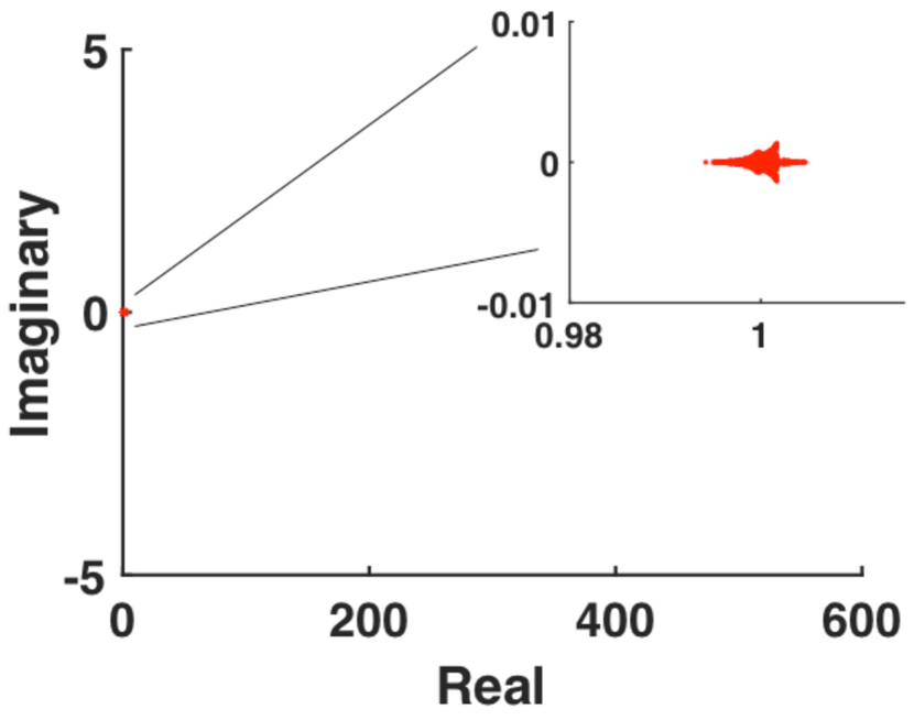
(a)

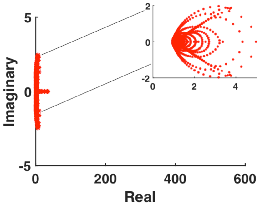
(b)

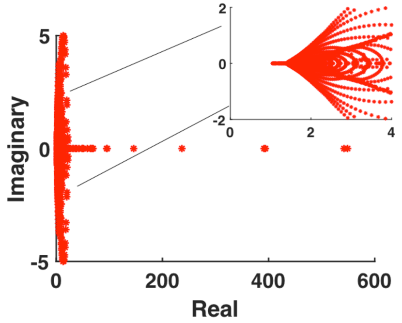
(c)

Fig. 5: Eigenvalues of preconditioned system 1/6 with (a) $\mathbf{P}_{5}$ recomputed, (b) $\mathbf{P}_{5}=\mathbf{N}_{5}\mathbf{P}_{1}$ (recycled), and (c) $\mathbf{P}_{1}$ reused. Note the different scale along the real axis compared with Figure 3 and 4.

5.3 Indefinite Matrices

In the previous tests, computing a new ILUTP for each system gives the lowest number of GMRES iterations, but it is too expensive in time. Here, we consider linear systems where the computation of the ILUTP preconditioner for the system of interest may fail or be unstable, resulting in poor preconditioners. This is the case, for example, for indefinite systems [88, Chapter 10]. We consider discretized 2D Helmholtz equations $-\Delta u-k^{2}u=f$, which arise in wave propagation problems [50, 51] and in flow control for unstable systems, giving eigenvalues in both the right- and left-half planes [35]. In such cases, we can select from the set (or more generally) a reference matrix for which the ILUTP algorithm computes an effective preconditioner and recycle this preconditioner using SAMs to (approximately) map matrices for which ILUTP may fail to the reference matrix.

Using a modified Helmholtz equation to compute a preconditioner has also been applied for other preconditioning approaches [51]. Previous work has successfully used operator-based preconditioners to achieve fast convergence for Krylov methods. The shifted Laplace preconditioner [51] is used along with multilevel Krylov methods in [50, 52, 90], while a sweeping preconditioner is constructed layer-by-layer in [49]. Preconditioning by replacing a subset of the Sommerfeld-type boundary conditions of the Helmholtz equation with Dirichlet or Neumann boundary conditions is examined in [47, 48]. We use this test problem just to demonstrate another possible use of SAMs; we do not consider whether this approach is competitive with the methods above.

We compute the matrix $\mathbf{K}_{0}$ and right hand side $\mathbf{b}$ by discretizing the 2D Laplacian on the unit square with Dirichlet boundary conditions, $u(x,0)=1$, $u(0,y)=1$, $u(x,1)=0$, and $u(1,y)=0$, using a vertex-centered finite volume discretization. $\mathbf{K}_{0}$ is symmetric, positive definite and has size $100\times 100$. We compute an ILUTP preconditioner, $\mathbf{P}_{0}$, for $\mathbf{K}_{0}$. Next, we solve the systems

$$\mathbf{K}_{i}=\mathbf{K}_{0}-s_{i}\mathbf{I},$$ (24)

where $\mathbf{I}$ is the identity matrix, and $s_{i}=i\Delta s$ with $\Delta s=0.01$, for $i=1,2,\dots,200$. We solve these systems with preconditioned full GMRES, comparing a new ILUTP preconditioner for every shift with recycling $\mathbf{P}_{0}$ using a SAM with the pattern of $\mathbf{K}_{0}$ for each system. The relative convergence tolerance is $10^{-10}$ and we use a zero initial guess for each system. For our ILUTP implementation, fill in is 20 and the drop tolerance is $10^{-3}$. For MATLAB^®’s ilu with type ‘ilutp’, the drop tolerance is $10^{-3}$.

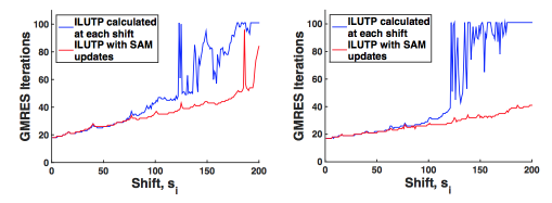
(a) Number of GMRES iterations to converge for the discretized Helmholtz equation, comparing a new ILUTP for each $\mathbf{K}_{i}$ (blue line) with recycling $\mathbf{P}_{0}$ using SAM updates for the $\mathbf{K}_{i}$ (red line). The results on the left are based on our ILUTP implementation. Those on the right are based on the MATLAB^® ilu preconditioner with type ‘ilutp’.

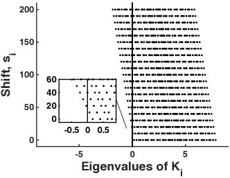
(b) Eigenvalues of every tenth matrix, $\mathbf{K}_{i}$. At the twentieth shift, the matrices become indefinite.

Fig. 6: GMRES convergence and selected eigenvalues for a discretized Helmholtz problem.

The results are presented in Figure 6(a). Figure 6(b) shows the eigenvalues for selected $\mathbf{K}_{i}$. While $\mathbf{K}_{i}$ becomes indefinite at the twentieth shift, ILUTP produces good preconditioners until about shift $s_{125}$. After this shift, both our ILUTP implementation and MATLAB^®’s $\tt ilu$ with type ‘ilutp’ fail to produce a good preconditioner, and the number of GMRES iterations increases substantially (or GMRES fails to converge). However, using SAM updates to recycle $\mathbf{P}_{0}$ keeps the GMRES iterations low for almost all shifts. For these small problems, we are not concerned with runtime and just demonstrate the superior convergence behavior obtained with the recycled preconditioners using SAMs compared with ILUTP.

6 Conclusions and Future Work

In applications that involve many linear systems, recycling a preconditioner can be advantageous, especially when computing a preconditioner from scratch is expensive. We develop a flexible update to arbitrary preconditioners that we call the Sparse Approximate Map, or SAM, update, which can be computed for any set of closely related matrices. The SAM is motivated by the Sparse Approximate Inverse; however, rather than approximately inverting a matrix, a SAM update approximately maps a matrix to a nearby matrix for which a good preconditioner is available. Using SAMs, the cost of computing a very good preconditioner can be amortized over many systems in a sequence, since computing SAMs is cheap. Further, a SAM is independent of preconditioner type and quality. The sparsity patterns for SAMs can be based on powers of $\mathbf{A}_{0}$, mesh-based patterns, or any other salient feature of a specific problem.

In future work, we plan to consider incremental SAM updates as in (17), applying maps from the left as in (18), and maps that allow CG and MINRES to be used. Another important future topic are approaches that update only a few columns or rows of the map to match localized changes in the matrix $\mathbf{A}_{k}$. More generally, we plan to consider maps that are tuned to various structural changes in a sequence of matrices that are known a priori. We also plan to develop more indicators for computing a new map. Finally, we plan to consider other types of maps, including different, potentially adaptive, choices in sparsity patterns.

7 Acknowledgements

We thank Xiaozhe Hu for sharing his MATLAB^®  implementation of the AMG preconditioner with us and for his advice how to incorporate it into our solvers. We also thank Tania Bakhos, Arvind Saibaba, and Peter Kitanidis for providing us with matrices from a THT application [11]. The application is not represented in the final draft of this paper, but it was very helpful in the development of our ideas. We further thank the anonymous reviewers for their suggestions, which led to several valuable improvements in this paper.

References

- [1] Alireza Aghasi, Misha E. Kilmer, and Eric L. Miller, Parametric level set methods for inverse problems, SIAM Journal on Imaging Sciences, 4 (2011), pp. 618–650.
- [2] Mian Ilyas Ahmad, Daniel B. Szyld, and Martin B. van Gijzen, Preconditioned multishift BiCG for H2-optimal model reduction, SIAM Journal on Matrix Analysis and Applications, 38 (2017), pp. 401–424.
- [3] Kapil Ahuja, Peter Benner, Eric de Sturler, and Lihong Feng, Recycling BiCGSTAB with an application to parametric model order reduction, SIAM Journal on Scientific Computing, 37 (2015), pp. S429–S446.
- [4] Kapil Ahuja, Bryan K. Clark, Eric de Sturler, David M. Ceperley, and Jeongnim Kim, Improved scaling for quantum Monte Carlo on insulators, SIAM Journal on Scientific Computing, 33 (2011), pp. 1837–1859.
- [5] Kapil Ahuja, Eric de Sturler, Serkan Gugercin, and Eun R. Chang, Recycling BiCG with an application to model reduction, SIAM Journal on Scientific Computing, 34 (2012), pp. A1925–A1949.
- [6] Athanasios C. Antoulas, Approximation of large-scale dynamical systems, SIAM, Philadelphia, PA, USA, 2005.
- [7] Athanasios C. Antoulas, Christopher A. Beattie, and Serkan Gugercin, Interpolatory model reduction of large-scale dynamical systems, in Efficient Modeling and Control of Large-Scale Systems, J. Mohammadpour and K. M. Grigoriadis, eds., Springer, 2010, pp. 3–58.
- [8] , Interpolatory Methods for Model Reduction, Computational Science and Engineering 21, SIAM, Philadelphia, 2020.
- [9] Hartwig Anzt, Edmond Chow, Jens Saak, and Jack Dongarra, Updating incomplete factorization preconditioners for model order reduction, Numerical Algorithms, 73 (2016), pp. 611–630.
- [10] Hartwig Anzt, Thomas Huckle, Jürgen Bräckle, and Jack Dongarra, Incomplete sparse approximate inverses for parallel preconditioning, Parallel Computing, 71 (2018), pp. 1–22.
- [11] Tania Bakhos, Arvind K. Saibaba, and Peter K. Kitanidis, A fast algorithm for parabolic PDE-based inverse problems based on Laplace transforms and flexible Krylov solvers, Journal of Computational Physics, 299 (2015), pp. 940–954.
- [12] Manuel Baumann and Martin B. van Gijzen, Nested Krylov methods for shifted linear systems, SIAM Journal on Scientific Computing, 37 (2015), pp. S90–S112.
- [13] Ulrike Baur, Peter Benner, and Lihong Feng, Model order reduction for linear and nonlinear systems: a system-theoretic perspective, Archives of Computational Methods in Engineering, 21 (2014), pp. 331–358.
- [14] Christopher A. Beattie and Serkan Gugercin, Realization-independent -approximation, in Proceedings of 51st IEEE Conference on Decision and Control, 2012, pp. 4953 – 4958.
- [15] Christopher A. Beattie, Serkan Gugercin, and Sarah A. Wyatt, Inexact solves in interpolatory model reduction, Linear Algebra and its Applications, 436 (2012), pp. 2916–2943.
- [16] Stefania Bellavia, Daniele Bertaccini, and Benedetta Morini, Nonsymmetric preconditioner updates in Newton-Krylov methods for nonlinear systems, SIAM Journal on Scientific Computing, 33 (2011), pp. 2595–2619.
- [17] Stefania Bellavia, Valentina De Simone, Daniela di Serafino, and Benedetta Morini, Efficient preconditioner updates for shifted linear systems, SIAM Journal on Scientific Computing, 33 (2011), pp. 1785–1809.
- [18] Martin P. Bendsøe, Optimal shape design as a material distribution problem, Structural Optimization, 1 (1989), pp. 193–202.
- [19] Martin P. Bendsøe, Aharon Ben-Tal, and Jochem Zowe, Optimization methods for truss geometry and topology design, Structural Optimization, 7 (1994), pp. 141–159.
- [20] Martin P. Bendsøe and Ole Sigmund, Material interpolation schemes in topology optimization, Archives of Applied Mechanics, 69 (1999), pp. 635–654.
- [21] Martin P. Bendsøe and Ole Sigmund, Topology optimization: theory, methods, and applications, Springer, Berlin, 2003.
- [22] Peter Benner, Serkan Gugercin, and Karen Willcox, A survey of projection-based model reduction methods for parametric dynamical systems, SIAM Review, 57 (2015), pp. 483–531.
- [23] Peter Benner, Mario Ohlberger, Albert Cohen, and Karen Willcox, Model Reduction and Approximation, Society for Industrial and Applied Mathematics, Philadelphia, PA, 2017.
- [24] Maurice W. Benson, Iterative solution of large scale linear systems, master’s thesis, Lakehead University, Thunder Bay, Canada, 1973.
- [25] Maurice W. Benson and Paul O. Frederickson, Iterative solution of large sparse linear systems arising in certain multidimensional approximation problems, Utilitas Mathematica, 22 (1982), pp. 127–140.
- [26] Michele Benzi, Preconditioning techniques for large linear systems: a survey, Journal of Computational Physics, 182 (2002), pp. 418–477.
- [27] Michele Benzi and Daniele Bertaccini, Approximate inverse preconditioning for shifted linear systems, BIT Numerical Mathematics, 43 (2003), pp. 231–244.
- [28] Michele Benzi, Jane K. Cullum, and Miroslav Tůma, Robust approximate inverse preconditioning for the conjugate gradient method, SIAM Journal on Scientific Computing, 22 (2000), pp. 1318–1332.
- [29] Michele Benzi, John C. Haws, and Miroslav Tůma, Preconditioning highly indefinite and nonsymmetric matrices, SIAM Journal on Scientific Computing, 22 (2000), pp. 1333–1353.
- [30] Michele Benzi, Reijo Kouhia, and Miroslav Tůma, Stabilized and block approximate inverse preconditioners for problems in solid and structural mechanics, Computer Methods in Applied Mechanics and Engineering, 190 (2001), pp. 6533–6554.
- [31] Michele Benzi and Miroslav Tůma, A sparse approximate inverse preconditioner for nonsymmetric linear systems, SIAM Journal on Scientific Computing, 19 (1998), pp. 968–994.
- [32] , A comparative study of sparse approximate inverse preconditioners, Applied Numerical Mathematics, 30 (1999), pp. 305–340.
- [33] Luca Bergamaschi, A survey of low-rank updates of preconditioners for sequences of symmetric linear systems, Algorithms, 13 (2020), p. 100.
- [34] Daniele Bertaccini, Efficient preconditioning for sequences of parametric complex symmetric linear systems, Electronic Transactions on Numerical Analysis, 18 (2004), pp. 49–64.
- [35] Jeffrey T. Borggaard and Serkan Gugercin, Model reduction for DAEs with an application to flow control 2014, in Active Flow and Combustion Control, R. King, ed., Springer International Publishing, 2015, pp. 381–396.
- [36] Rafael Bru, José Marín, José Mas, and Miroslav Tůma, Balanced incomplete factorization, SIAM Journal on Scientific Computing, 30 (2008), pp. 2302–231.
- [37] Angelika Bunse-Gerstner, Dorota Kubalińska, Georg Vossen, and Daniel Wilczek, -optimal model reduction for large scale discrete dynamical MIMO systems, Journal of Computational and Applied Mathematics, (2009). doi:10.1016/j.cam.2008.12.029.
- [38] Caterina Calgaro, Jean-Paul Chehab, and Yousef Saad, Incremental incomplete LU factorizations with applications, Numerical Linear Algebra with Applications, 17 (2010), pp. 811–837.
- [39] Michael Cardiff and Warren Barrash, 3-D Transient hydraulic tomography in unconfined aquifers with fast drainage response, Water Resources Research, 47 (2011).
- [40] Juana Cerdán, José Marín, and José Mas, Low-rank updates of balanced incomplete factorization preconditioners, Numerical Algorithms, 74 (2017), pp. 337–370.
- [41] Edmond Chow, A priori sparsity patterns for parallel sparse approximate inverse preconditioners, SIAM Journal on Scientific Computing, 21 (2000), pp. 1804–1822.
- [42] , Parallel implementation and practical use of sparse approximate inverse preconditioners with a priori sparsity patterns, International Journal of High Performance Computing Applications, 15 (2001), pp. 56–74.
- [43] Edmond Chow and Aftab Patel, Fine-grained parallel incomplete LU factorization, SIAM Journal on Scientific Computing, 37 (2015), pp. C169–C193.
- [44] Edmond Chow and Yousef Saad, Approximate inverse preconditioners via sparse-sparse iterations, SIAM Journal on Scientific Computing, 19 (1998), pp. 995–1023.
- [45] Eric de Sturler and Misha E. Kilmer, A regularized Gauss-Newton trust region approach to imaging in diffuse optical tomography, SIAM Journal on Scientific Computing, 33 (2011), pp. 3057–3086.
- [46] Harry Dym, Linear Algebra in Action, American Mathematical Society, 2 ed., 2013.
- [47] Howard C. Elman and Dianne P. O’Leary, Efficient iterative solution of the three-dimensional Helmholtz equation, Journal of Computational Physics, 142 (1998), pp. 163–181.
- [48] , Eigenanalysis of some preconditioned Helmholtz problems, Numerische Mathematik, 83 (1999), pp. 231–257.
- [49] Björn Engquist and Lexing Ying, Sweeping preconditioner for the Helmholtz equation: hierarchical matrix representation, Communications on Pure and Applied Mathematics, 64 (2011), pp. 697–735.
- [50] Yogi A. Erlangga and Reinhard Nabben, On a multilevel Krylov method for the Helmholtz equation preconditioned by shifted Laplacian, Electronic Transactions on Numerical Analysis, 31 (2008), pp. 403–424.
- [51] Yogi A. Erlangga, Cornelis Vuik, and Cornelis W. Oosterlee, On a class of preconditioners for solving the Helmholtz equation, Applied Numerical Mathematics, 50 (2004), pp. 409–425.
- [52] , Comparison of multigrid and incomplete LU shifted-Laplace preconditioners for the inhomogeneous Helmholtz equation, Applied Numerical Mathematics, 56 (2006), pp. 648–666.
- [53] Lihong Feng, Peter Benner, and Jan G. Korvink, Parametric model order reduction accelerated by subspace recycling, in 48th IEEE Conference on Decision & Control and 28th Chinese Control Conference, 2009, pp. 4328–4333.
- [54] , Subspace recycling accelerates the parametric macro-modeling of MEMS, International Journal for Numerical Methods in Engineering, 94 (2013), pp. 84–110.
- [55] G.H. Golub and C.F. Van Loan, Matrix Computations, Johns Hopkins University Press, 3 ed., 1996.
- [56] Andrew D. Gordon and Catherine E. Powell, On solving stochastic collocation systems with algebraic multigrid, IMA Journal of Numerical Analysis, 32 (2012), pp. 1051–1070.
- [57] Anne Greenbaum, Iterative Methods for Solving Linear Systems, SIAM, Philadelphia, PA, 1997.
- [58] Arielle Grim-McNally and Eric de Sturler, MATLAB® implementation of Yousef Saad’s ILUTP algorithm. Available from https://arxiv.org/abs/1601.05883, 2016. This implementation closely follows the ILUT paper and SPARSKIT, while exploiting several steps to ensure an efficient implementation in MATLAB (R).
- [59] Arielle Grim-McNally, Eric de Sturler, and Serkan Gugercin, Preconditioning parametrized linear systems. Available from https://arxiv.org/abs/1601.05883, 2020. This is a previous, unpublished version of the current paper containing more detailed descriptions of the sparsity patterns considered in Section 3.
- [60] Marcus J. Grote and Thomas Huckle, Effective parallel preconditioning, in Proceedings of the Seventh SIAM Conference on Parallel Processing for Scientific Computing, PPSC 1995, San Francisco, California, USA, February 15-17, 1995, David H. Bailey, Petter E. Bjørstad, John R. Gilbert, Michael Mascagni, Robert S. Schreiber, Horst D. Simon, Virginia Torczon, and Layne T. Watson, eds., SIAM, 1995, pp. 466–471.
- [61] , Parallel preconditioning with sparse approximate inverses, SIAM Journal on Scientific Computing, 18 (1997), pp. 838–853.
- [62] Guiding Gu, Xianli Zhou, and Lei Lin, A flexible preconditioned Arnoldi method for shifted linear systems, Journal of Computational Mathematics, 25 (2007), pp. 522–530.
- [63] Serkan Gugercin, Athanasios C. Antoulas, and Christopher A. Beattie, H2 model reduction for large-scale linear dynamical systems, SIAM Journal on Matrix Analysis and Applications, 30 (2008), pp. 609–638.
- [64] Jan S. Hesthaven, Gianluigi Rozza, and Benjamin Stamm, Certified reduced basis methods for parametrized partial differential equations, Springer Briefs in Mathematics, Springer, Switzerland, 2016.
- [65] Jeffrey Hokanson and Caleb Magruder, -optimal model reduction using projected nonlinear least squares, (2018).
- [66] Ruth M. Holland, Andy J. Wathen, and Gareth J. Shaw, Sparse approximate inverses and target matrices, SIAM Journal on Scientific Computing, 26 (2005), pp. 1000–1011.
- [67] Xiaozhe Hu, Junyuan Lin, and Ludmil T. Zikatanov, An adaptive multigrid method based on path cover, SIAM Journal on Scientific Computing, 41 (2019), pp. S220–S241.
- [68] Thomas Huckle, Approximate sparsity patterns for the inverse of a matrix and preconditioning, Applied Numerical Mathematics, 30 (1999), pp. 291–303.
- [69] , Factorized sparse approximate inverses for preconditioning, The Journal of Supercomputing, 25 (2003), pp. 109–117.
- [70] Thomas Huckle and Alexander Kallischko, Frobenius norm minimization and probing for preconditioning, International Journal of Computer Mathematics, 84 (2007), pp. 1225 – 1248.
- [71] Thomas Huckle, Alexander Kallischko, Andreas Roy, Matous Sedlacek, and Tobias Weinzierl, An efficient parallel implementation of the MSPAI preconditioner, Parallel Computing, 36 (2010), pp. 273–284.
- [72] Thomas K. Huckle, Efficient computation of sparse approximate inverses, Numerical Linear Algebra with Applications, 5 (1998), pp. 57–71.
- [73] Alexander Kallischko, Modified sparse approximate inverses (MSPAI) for parallel preconditioning, PhD thesis, Technische Universitat Munchen, 2008. Advisor: Thomas Huckle.
- [74] Misha E. Kilmer and Eric de Sturler, Recycling subspace information for diffuse optical tomography, SIAM Journal on Scientific Computing, 27 (2006), pp. 2140–2166.
- [75] Evgenii B. Korvink, Jan G.and Rudnyi, Oberwolfach benchmark collection, in Dimension Reduction of Large-Scale Systems, Peter Benner, Daniel C. Sorensen, and Volker Mehrmann, eds., Berlin, Heidelberg, 2005, Springer Berlin Heidelberg, pp. 311–315.
- [76] Jaroslav Mackerle, Topology and shape optimization of structures using FEM and BEM: A bibliography (1999–2001), Finite Elements in Analysis and Design, 39 (2003), pp. 243–253.
- [77] Christian Moosmann, Evgenii B. Rudnyi, Andreas Greiner, and Jan G. Korvink, Model order reduction for linear convective thermal flow, in Proceedings of 10th International Workshops on THERMal INvestigations of ICs and Systems, vol. 29, 2004, pp. 317–322.
- [78] The MORwiki Community, Convection. MORwiki – Model Order Reduction Wiki, http://modelreduction.org/index.php/Convection, 2020.
- [79] Alfio Quarteroni, Andrea Manzoni, and Federico Negri, Reduced basis methods for partial differential equations: an introduction, vol. 92, Springer, 2015.
- [80] Amin Rafiei, Left-looking version of AINV preconditioner with complete pivoting strategy, Linear Algebra and its Applications, 445 (2014), pp. 103–126.
- [81] G. I. N. Rozvany, Aims, scope, methods, history and unified terminology of computer-aided topology optimization in structural mechanics, Structural and Multidisciplinary Optimization, 21 (2001), pp. 90–108.
- [82] G. I. N. Rozvany, Martin P. Bendsøe, and Uri Kirsch, Layout optimization of structures, Applied Mechanics Reviews, 48 (1995), pp. 41–119.
- [83] Evgenii B. Rudnyi and Jan G. Korvink, Review: Automatic model reduction for transient simulation of MEMS-based devices, Sensors Update, 11 (2002), pp. 3–33.
- [84] John W. Ruge and Klaus Stüben, Efficient solution of finite difference and finite element equations by algebraic multigrid (AMG), in Multigrid methods for integral and differential equations, The Institute of Mathematics and its applications conference series, H. Holstein D.J. Paddon, ed., vol. 3, Clarendon Press, Oxford, 1985, pp. 169–212.
- [85] , Algebraic multigrid (AMG), in Multigrid Methods (Frontiers in Applied Mathematics), S.F. McCormick, ed., SIAM, Philadelphia, 1986.
- [86] Yousef Saad, ILUT: a dual threshold incomplete LU factorization, Numerical Linear Algebra with Applications, 1 (1994), pp. 387–402.
- [87] , SPARSKIT: A basic took-kit for sparse matrix computations. http://www-users.cs.umn.edu/ saad/software/SPARSKIT/, 1994.
- [88] , Iterative Methods for Sparse Linear Systems, 2nd Ed., SIAM, 2003.
- [89] Arvind K. Saibaba, Tania Bakhos, and Peter K. Kitanidis, A flexible Krylov solver for shifted systems with application to oscillatory hydraulic tomography, SIAM Journal on Scientific Computing, 35 (2013), pp. A3001–A3023.
- [90] Abdul H. Sheikh, Domenico Lahaye, and Cornelis Vuik, On the convergence of shifted Laplace preconditioner combined with multilevel deflation, Numerical Linear Algebra with Applications, 20 (2013), pp. 645–662.
- [91] Ole Sigmund, Topology optimization: a tool for the tailoring of structures and materials, Philosophical Transactions: Mathematical, Physical and Engineering Sciences, 358 (2000), pp. 211–228.
- [92] Klaus Stüben, Algebraic multigrid (AMG): Experiences and comparisons, Applied Mathematics and Computation, 13 (1983), pp. 419–452.
- [93] Klaus Stüben, Algebraic multigrid (AMG): an introduction with applications, in Multigrid, New York Academic Press, ed., Trottenberg, Ulrich and Oosterlee, Cornelius W and Schüller, Anton, 2000.
- [94] Klaus Stüben, A review of algebraic multigrid, Journal of Computational and Applied Mathematics, 128 (2001), pp. 281–309.
- [95] Wei-Pai Tang, Toward an effective sparse approximate preconditioner, SIAM Journal on Matrix analysis and applications, 20 (1999), pp. 970–986.
- [96] Jurjen Duintjer Tebbens and Miroslav Tůma, Preconditioner updates for solving sequences of linear systems in a matrix-free environment, Numerical Linear Algebra with Applications, 17 (2010), pp. 997–1019.
- [97] Ulrich Trottenberg, Cornelius W Oosterlee, and Anton Schüller, Multigrid, Elsevier, 2000.
- [98] Shun Wang, Krylov Subspace Methods for Topology Optimization on Adaptive Meshes, PhD thesis, Univeristy of Illinois at Urbana-Champaign, 2007. Advisor Eric de Sturler.
- [99] Shun Wang and Eric de Sturler, Multilevel sparse approximate inverse preconditioners for adaptive mesh refinement, Linear Algebra and its Applications, 431 (2009), pp. 409–426.
- [100] Shun Wang, Eric de Sturler, and Glaucio H. Paulino, Large-scale topology optimization using preconditioned Krylov subspace methods with recycling, International Journal for Numerical Methods in Engineering, 69 (2007), pp. 2441–2468.
- [101] Sarah A. Wyatt, Issues in interpolatory model reduction: Inexact solves, second-order systems and DAEs, PhD thesis, Virginia Tech, 2012.
- [102] Yuesheng Xu and Taishan Zeng, Optimal model reduction for large scale MIMO systems via tangential interpolation, International Journal of Numerical Analysis and Modeling, 8 (2011), pp. 174–188.