MORPHOLOGICAL PROPERTIES OF LYMAN $\alpha$ EMITTERS AT REDSHIFT 4.86 IN THE COSMOS FIELD: CLUMPY STAR FORMATION OR MERGER?

Abstract

We investigate morphological properties of 61 Ly$\alpha$ emitters (LAEs) at $z=4.86$ identified in the COSMOS field, based on Hubble Space Telescope Advanced Camera for Surveys (ACS) imaging data in the F814W-band. Out of the 61 LAEs, we find the ACS counterparts for the 54 LAEs. Eight LAEs show double-component structures with a mean projected separation of 0$\farcs$63 ($\sim 4.0$ kpc at $z=4.86$). Considering the faintness of these ACS sources, we carefully evaluate their morphological properties, that is, size and ellipticity. While some of them are compact and indistinguishable from the PSF half-light radius of 0$\farcs$07 ($\sim 0.45$ kpc), the others are clearly larger than the PSF size and spatially extended up to 0$\farcs$3 ($\sim 1.9$ kpc). We find that the ACS sources show a positive correlation between ellipticity and size and that the ACS sources with large size and round shape are absent. Our Monte Carlo simulation suggests that the correlation can be explained by (1) the deformation effects via PSF broadening and shot noise or (2) the source blending in which two or more sources with small separation are blended in our ACS image and detected as a single elongated source. Therefore, the 46 single-component LAEs could contain the sources which consist of double (or multiple) components with small spatial separation (i.e., $\lesssim 0\farcs 3$ or 1.9 kpc). Further observation with high angular resolution at longer wavelengths (e.g., rest-frame wavelengths of $\gtrsim 4000$ Å) is inevitable to decipher which interpretation is adequate for our LAE sample.

1. INTRODUCTION

In the standard picture of structure formation, within the framework of Cold Dark Matter (CDM) models, small subgalactic clumps are formed first in CDM halos. Such building blocks of normal galaxies in local universe grow hierarchically into more massive galaxies through galaxy mergers and subsequent star formation. Ly$\alpha$ emitters (LAEs) at high-$z$ universe are considered to be building blocks because of their small stellar masses, young ages, and low metallicities inferred from their broadband spectral energy distributions (e.g., Chary et al. 2005; Gawiser et al. 2006; Nilsson et al. 2007, 2009; Finkelstein et al. 2008; Ono et al. 2010a, b; Yuma et al. 2010; Acquaviva et al. 2011; Guaita et al. 2011; Vargas et al. 2014). Since they are important population as a probe of galaxy formation in the young universe as well as a probe of cosmic reionization, much effort has been paid to search them (e.g., Cowie & Hu 1998; Rhoads et al. 2000; Ouchi et al. 2005, 2008, 2010; Taniguchi et al. 2005; Shimasaku et al. 2006; Gronwall et al. 2007; Murayama et al. 2007; Shioya et al. 2009; Kashikawa et al. 2011). The redshift of the most distant LAE has now reached beyond $z=7$ (Ono et al. 2012; Shibuya et al. 2012; Finkelstein et al. 2013), at which cosmic reionization has not been completed yet.

However, it is still unclear in what physical conditions a galaxy is observed as an LAE, which has intense Ly$\alpha$ emission. This is mainly because Ly$\alpha$ is a resonance line of neutral hydrogen; that is, mean free path of Ly$\alpha$ photon in interstellar medium (ISM) is significantly short and hence it experiences enormous number of scattering by neutral hydrogen before escaping from its host galaxy. The multiple scattering makes Ly$\alpha$ extremely vulnerable to dust attenuation. This is consistent with the observational results for the LAEs in both nearby and high-$z$ universe which have revealed that the Ly$\alpha$ escape fraction depends clearly on dust extinction, although the escape fraction does not follow the expected one for a simple attenuation (Atek et al. 2009, 2014; Kornei et al. 2010; Hayes et al. 2011, 2014). Theoretical studies have also been executed, in which Ly$\alpha$ radiative transfer code is coupled with cosmological numerical simulation in order to examine the Ly$\alpha$ escape fraction in realistic ISM condition for high-$z$ LAE (e.g., Laursen & Sommer-Larsen 2007; Laursen et al. 2009a, b; Zheng et al. 2010; Yajima et al. 2012a, b). These theoretical studies predict that ISM clumpiness and morphology have a strong impact on Ly$\alpha$ escape fraction and that clumpy and dusty ISM is favored for Ly$\alpha$ to escape (Yajima et al. 2012b; Laursen et al. 2013; Duval et al. 2014; Gronke & Dijkstra 2014). Moreover, such clumpy and dusty ISM is also found to be favored to reproduce the observed statistical properties of LAEs (Kobayashi et al. 2007, 2010).

In such context, observational studies for the size and morphology of high-$z$ LAEs have been widely conducted by using the Advanced Camera for Surveys (ACS) on-board the Hubble Space Telescope (HST) because these properties give us insights on how LAEs are assembled and how their intense star formation events are triggered (e.g., Stanway et al. 2004; Rhoads et al. 2005; Venemans et al. 2005; Pirzkal et al. 2007; Overzier et al. 2008; Bond et al. 2009, 2012; Taniguchi et al. 2009; Vanzella et al. 2009; Finkelstein et al. 2011; Law et al. 2012; Malhotra et al. 2012; Mawatari et al. 2012; Chonis et al. 2013; Jiang et al. 2013; Hagen et al. 2014; Shibuya et al. 2014). It has been found that most of the high-$z$ LAEs have small sizes of 0$\farcs$1–0$\farcs$2 in rest-frame ultraviolet (UV) continuum, which remain almost constant in the redshift range of $z\sim 2$–6 (Malhotra et al. 2012; Hagen et al. 2014). This is against the hypothesis that LAE is simply a subset of Lyman-break galaxy (LBG) population, which present a clear redshift evolution of size in rest-frame UV continuum (e.g., Ono et al. 2013).

In this paper, we examine the morphological properties of the 61 LAEs at $z=4.86$ selected by Shioya et al. (2009; hereafter S09) in the Cosmic Evolution Survey (COSMOS) field (Scoville et al. 2007a), providing one of the largest samples of LAEs in a large contiguous field. Since F814W-band imaging taken with the HST/ACS is available for the COSMOS field (Scoville et al. 2007b; Koekemoer et al. 2007), the sizes and morphologies of the LAEs in the COSMOS field can be investigated in detail. In this paper, we present our detailed analysis of ACS images of the LAE sample of S09.

We use a standard cosmology with $\Omega_{M}=0.3$, $\Omega_{\Lambda}=0.7$, and $H_{0}=70~{}\mathrm{km~{}s^{-1}~{}Mpc^{-1}}$. Under the adopted cosmological parameters, the angular scale of $1^{\prime\prime}$ corresponds to the physical scale of 6.37 kpc at $z=4.86$. Throughout this paper, we use magnitudes in the AB system.

2. OBSERVATIONAL DATA AND ACS COUNTERPARTS OF LAEs

In S09, 79 LAE candidates at $4.83<z<4.89$ have been carefully selected from optical imaging with the narrow-band filter, NB711 ($\lambda_{\mathrm{c}}=7126$ Å, $\Delta\lambda=73$ Å; see Figure 1), and broad-band filters from $B$ to $z^{\prime}$ taken for the entire $1.95~{}\mathrm{deg^{2}}$ area of the COSMOS field using the Suprime-Cam (Miyazaki et al. 2002) on the Subaru Telescope (Kaifu et al. 2000; Iye et al. 2004). Details of the Subaru observations and data processing are described by Taniguchi et al. (2007) and Capak et al. (2007). Among 79 LAEs, 13 LAEs have spectroscopic information and all of them are confirmed as $z\approx 4.86$ (P. Capak et al. 2015, in preparation), verifying the effectiveness of our selection method.

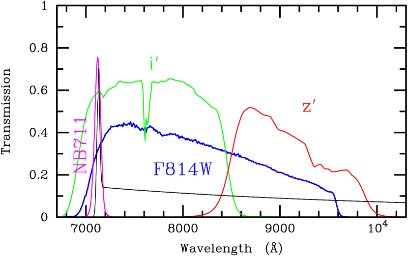
Figure 1.— Transmission curves for the filters related to our analysis. The blue curve represents the transmission curve for the HST/ACS F814W-band, while the magenta, green, and red curves are the transmissions for the Subaru/Suprime-Cam NB711–, $i^{\prime}$–, and $z^{\prime}$–bands, respectively. The effects of the CCD sensitivity, the atmospheric transmission, and the transmission of the telescope and the instrument are taken into account for each transmission curve. Model spectrum of a LAE at $z=4.86$ with a rest-frame Ly$\alpha$ equivalent width ($\mathrm{EW_{0}}$) of 30 Å is also plotted by black curve.

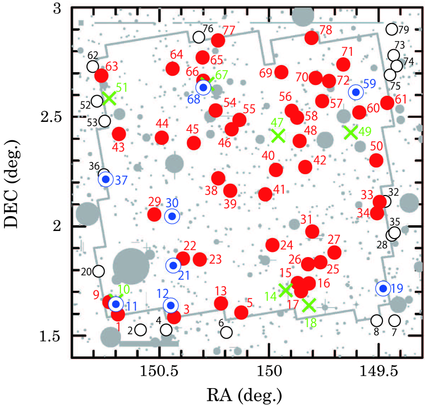
Figure 2.— Spatial distribution of our sample of 79 LAEs at $z=4.86$ selected in S09. In the whole COSMOS field of $1.95~{}\mathrm{deg}^{2}$, the HST/ACS images are available for $1.64~{}\mathrm{deg}^{2}$ indicated by the solid gray line. The gray shaded regions represent the areas masked out for detection. The 18 LAEs outside the HST/ACS field are shown by black open circles. Among the remaining 61 LAEs in the HST/ACS field, 7 LAEs undetected in the ACS images are represented by green crosses and 46 (8) LAEs with single (double) component(s) are shown by red filled (blue double) circles. The ID # in S09 is labeled for reference.

Table 1SExtractor configuration for the HST/ACS F814W-band detection

Parameter	Value	Comment
DETECT_THRESH	1.1	Detection threshold in sigma
DETECT_MINAREA	25	Minimum number of pixels above threshold
FILTER_NAME	gauss_3.0_7x7.conv	Name of the filter for detection
DEBLEND_NTHRESH	64	Number of deblending sub-thresholds
DEBLEND_MINCONT	0.015	Minimum contrast parameter for deblending
PHOT_AUTOPARAMS	2.5, 0.5	MAG_AUTO parameters: Kron factor and minimum radius
BACK_SIZE	64	Background mesh size
BACK_FILTERSIZE	3	Background filter size
BACKPHOTO_TYPE	GLOBAL	Photometry background subtraction type

The HST/ACS F814W-band data ($\lambda_{\mathrm{c}}=8333$ Å, $\Delta\lambda=2511$ Å; see Figure 1) is available for a part of the COSMOS field, $1.64~{}\mathrm{deg^{2}}$ ($\approx 84$% of the COSMOS field), as shown in Figure 2. In our analysis, we use the official COSMOS ACS image (Scoville et al. 2007b; Koekemoer et al. 2007), Version 2.0. The ACS data were processed to $0\farcs 03~{}\mathrm{pixel}^{-1}$ images. We find that ACS imaging data are available for 61 LAEs out of 79 LAE samples selected by S09. The remaining 18 LAEs are not covered by the ACS field or are on the edge of the ACS field. Spatial distribution of all 79 LAEs in the COSMOS field is shown in Figure 2. Our data analysis procedure for ACS data are similar to those in Taniguchi et al. (2009), in which the official COSMOS ACS image Version 1.3 with the pixel scale of $0\farcs 05~{}\mathrm{pixel}^{-1}$ was utilized. The source detection of the LAEs in the HST/ACS image was carried out with their weight map using SExtractor (Bertin & Arnouts 1996). The fundamental parameters of the SExtractor’s configuration are shown in Table 1, which are also basically similar to those used in Taniguchi et al. (2009) and modified slightly for the $0\farcs 03~{}\mathrm{pixel}^{-1}$ images. Note that these parameters are determined by the tradeoff between detecting fainter objects/components and avoiding noise effects such as the false detection or the noise confusion.

Table 2COSMOS $z=4.86$ LAE Sample

LAE Sample			Number of LAEs	Spectroscopic
				Confirmation
In the ACS/F814W-band field			61	13
	ACS/F814W-band detected		54	12
		Single component	46	10
		Double component	8	2
	ACS/F814W-band undetected		7	1
Out of the ACS/F814W-band field			18	0
Total			79	13

Among the 61 LAEs in the ACS field, we find the ACS counterparts of the 54 LAEs detected near the LAE positions defined in NB711–band images (i.e., separation of $\leq 1^{\prime\prime}$). Any sources are not detected near the LAE positions for the remaining seven LAEs. While most of the ACS counterparts consist of single component, eight LAEs among the 54 ACS-detected LAEs have double components in the ACS images within separation of $\leq 1^{\prime\prime}$ from the LAE positions, providing the double-component LAE fraction, $f_{\mathrm{double}}$, of $8/54=14.8$%. The numbers of the total sample, both the ACS-detected and undetected LAEs, are summarized in Table 2.

Separations between each component in the 8 double-component LAEs are found to be 0$\farcs$36–0$\farcs$98 (the mean is 0$\farcs$63). For these double-component LAEs, the mean offset of the ACS centroids from the NB711–band centroids is found to be 0$\farcs$39, which is larger than the NB711–band pixel scale of $0\farcs 15~{}\mathrm{pixel}^{-1}$. This is possibly because these double ACS components are unresolved in the NB711–band images taken by the Subaru telescope, in which the mean half-light radius of unsaturated stars is 0$\farcs$25, and their NB711–band positions can be close to their flux-weighted centroid. On the other hand, for the 46 single-component LAEs, the mean offset between the ACS F814W- and NB711–band centroids is 0$\farcs$16, which is comparable to the pixel scale of the NB711–band images. We note that, in the following analysis, the double ACS components in each one of the 8 double-component LAEs are treated as sub-components in a single object at first and the morphological properties of the objects are measured. The results with each of the components in the double component systems treated separately as different objects with close angular separation are presented in Section 3.4.

As shown in Figure 2, the ACS-detected (filled and double circles) and ACS-undetected LAEs (crosses) seem to be distributed randomly in the whole ACS field. Therefore, their distributions may not be affected by large-scale inhomogeneity of the ACS data quality (e.g., edges of the field). It should be noted that the LAE #20 is on the edge of the ACS field as shown in Figure 2. While the LAE #20 seems to have a double-component ACS source, we do not include it in our sample of the ACS-detected LAEs since the ACS data quality is highly doubtful.

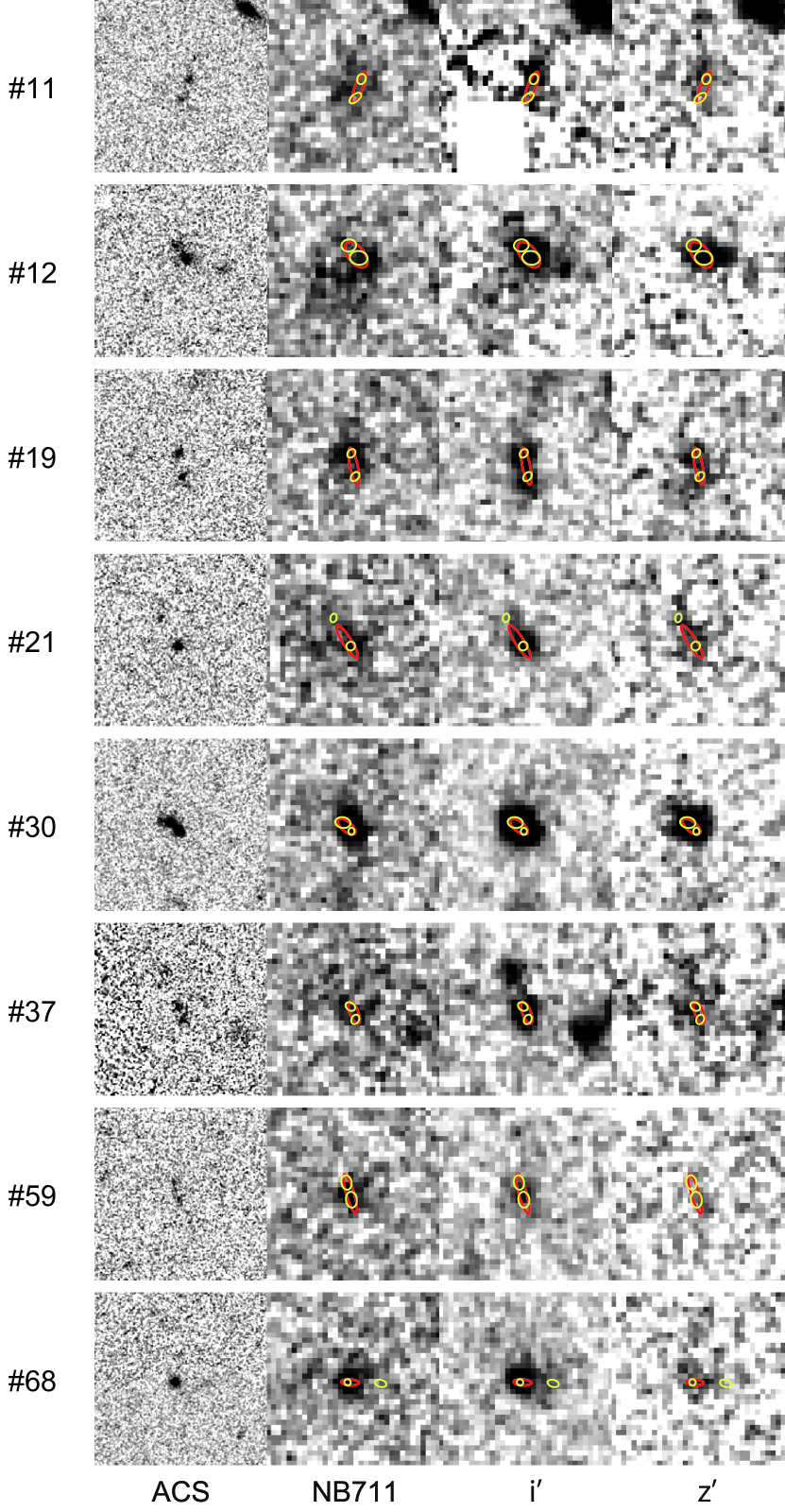
Figure 3.— Thumbnails of 8 LAEs with double-component ACS F814W-band sources. North is up and east is left. Each panel has a size of $5^{\prime\prime}\times 5^{\prime\prime}$. Red ellipses overplotted on the NB711– and $z^{\prime}$–band images are half light ellipses of the detected LAE counterparts in the ACS image, while yellow ellipses are those of the individual components in each LAE counterpart detected by SExtractor.

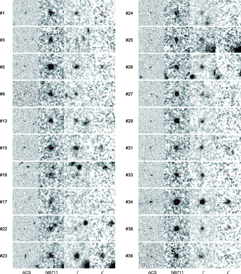
Figure 4.— Same as Figure 3 but for 46 LAEs with single component ACS source.

Figure 4.— (Continued.)

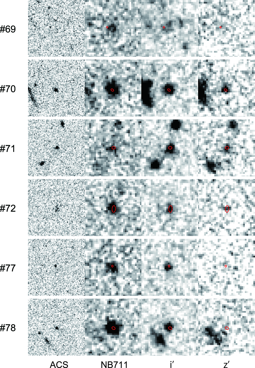
Figure 4.— (Continued.)

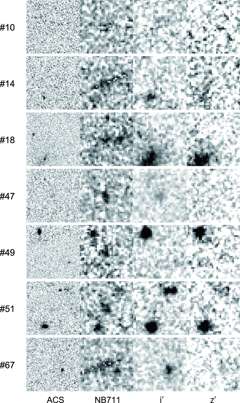
Figure 5.— Same as Figure 3 but for 7 LAEs without ACS sources.

Table 3ACS F814W-band Properties for the 61 LAEs at $z=4.86$ with ACS Data

ID	$I_{814}$	$a_{\mathrm{HL}}$	$R_{\mathrm{HL}}$	$\epsilon(I_{814})$	$NB711$	$a_{\mathrm{HL}}(\mathrm{NB711})$	$i^{\prime}$	$z^{\prime}$	$L(\mathrm{Ly\alpha})$	$\mathrm{EW_{0}}$	$z_{\mathrm{spec}}$
	(mag)	(arcsec)	(arcsec)		(mag)	(arcsec)	(mag)	(mag)	($10^{42}~{}\mathrm{erg~{}s^{-1}}$)	(Å)
8 ACS-detected LAEs with Double Components
11	$25.52\pm 0.06$	$0.49\pm 0.02$	$0.32\pm 0.02$	$0.76\pm 0.01$	$24.55\pm 0.18$	$0.51$	$25.73\pm 0.42$	$24.98\pm 0.24$	$5.6\pm 1.3$	$18\pm 6$	$-99.0$
12	$24.11\pm 0.03$	$0.44\pm 0.02$	$0.34\pm 0.01$	$0.47\pm 0.02$	$23.64\pm 0.08$	$1.02$	$24.16\pm 0.07$	$24.31\pm 0.13$	$9.5\pm 1.2$	$16\pm 3$	4.850
19	$25.06\pm 0.04$	$0.55\pm 0.02$	$0.37\pm 0.02$	$0.79\pm 0.01$	$24.18\pm 0.13$	$0.47$	$24.90\pm 0.10$	$24.82\pm 0.17$	$6.4\pm 1.1$	$18\pm 4$	$\cdots$
21	$25.05\pm 0.04$	$0.56\pm 0.04$	$0.24\pm 0.01$	$0.77\pm 0.01$	$23.96\pm 0.12$	$1.05$	$25.26\pm 0.12$	$24.83\pm 0.18$	$10.1\pm 1.3$	$28\pm 6$	$\cdots$
30	$23.87\pm 0.01$	$0.31\pm 0.00$	$0.25\pm 0.01$	$0.54\pm 0.01$	$23.50\pm 0.07$	$0.56$	$24.17\pm 0.05$	$24.13\pm 0.09$	$11.7\pm 1.1$	$17\pm 2$	$\cdots$
37	$25.21\pm 0.06$	$0.34\pm 0.02$	$0.23\pm 0.01$	$0.64\pm 0.02$	$24.08\pm 0.13$	$0.76$	$24.59\pm 0.07$	$24.31\pm 0.11$	$5.8\pm 1.2$	$10\pm 2$	$\cdots$
59	$25.47\pm 0.07$	$0.59\pm 0.05$	$0.32\pm 0.03$	$0.81\pm 0.02$	$24.52\pm 0.17$	$0.54$	$25.52\pm 0.14$	$26.03\pm 0.47$	$5.4\pm 1.1$	$45\pm 26$	$\cdots$
68	$25.02\pm 0.02$	$0.25\pm 0.01$	$0.13\pm 0.00$	$0.65\pm 0.01$	$24.06\pm 0.12$	$0.86$	$24.65\pm 0.07$	$25.12\pm 0.22$	$6.5\pm 1.1$	$24\pm 7$	4.798
46 ACS-detected LAEs with Single Component
1	$26.20\pm 0.10$	$0.17\pm 0.01$	$0.13\pm 0.01$	$0.49\pm 0.04$	$24.86\pm 0.26$	$0.40$	$26.54\pm 0.32$	$25.95\pm 0.46$	$4.8\pm 1.2$	$38\pm 22$	$-99.0$
3	$26.79\pm 0.11$	$0.11\pm 0.01$	$0.10\pm 0.01$	$0.13\pm 0.11$	$24.46\pm 0.20$	$0.37$	$26.38\pm 0.31$	$>26.64$	$7.1\pm 1.3$	$>105$	$\cdots$
5	$26.27\pm 0.07$	$0.10\pm 0.01$	$0.10\pm 0.01$	$0.13\pm 0.07$	$23.43\pm 0.07$	$0.53$	$25.63\pm 0.15$	$25.61\pm 0.29$	$19.0\pm 1.1$	$109\pm 34$	4.839
9	$27.30\pm 0.10$	$0.08\pm 0.01$	$0.06\pm 0.00$	$0.37\pm 0.09$	$24.22\pm 0.13$	$0.58$	$26.02\pm 0.21$	$>26.64$	$8.8\pm 1.1$	$>130$	$\cdots$
13	$26.97\pm 0.07$	$0.09\pm 0.00$	$0.08\pm 0.00$	$0.24\pm 0.08$	$24.71\pm 0.20$	$0.44$	$25.97\pm 0.19$	$25.67\pm 0.31$	$5.0\pm 1.1$	$30\pm 12$	$\cdots$
15	$25.73\pm 0.06$	$0.12\pm 0.01$	$0.12\pm 0.01$	$0.06\pm 0.06$	$24.07\pm 0.12$	$1.02$	$25.18\pm 0.11$	$25.43\pm 0.27$	$8.7\pm 1.2$	$42\pm 13$	$\cdots$
16	$27.26\pm 0.16$	$0.09\pm 0.01$	$0.08\pm 0.02$	$0.13\pm 0.14$	$24.46\pm 0.17$	$0.60$	$25.43\pm 0.13$	$25.87\pm 0.39$	$5.4\pm 1.1$	$39\pm 19$	$\cdots$
17	$27.09\pm 0.16$	$0.12\pm 0.02$	$0.11\pm 0.01$	$0.13\pm 0.16$	$24.74\pm 0.22$	$0.59$	$26.76\pm 0.40$	$>26.64$	$5.6\pm 1.2$	$>83$	$\cdots$
22	$27.00\pm 0.11$	$0.09\pm 0.01$	$0.08\pm 0.01$	$0.21\pm 0.08$	$24.51\pm 0.17$	$0.90$	$26.36\pm 0.24$	$>26.64$	$6.8\pm 2.8$	$>101$	$\cdots$
23	$25.33\pm 0.04$	$0.23\pm 0.00$	$0.16\pm 0.01$	$0.56\pm 0.02$	$24.41\pm 0.15$	$0.42$	$24.94\pm 0.08$	$24.73\pm 0.15$	$4.5\pm 1.0$	$11\pm 3$	$\cdots$
24	$26.54\pm 0.10$	$0.12\pm 0.01$	$0.11\pm 0.01$	$0.24\pm 0.06$	$24.49\pm 0.18$	$0.62$	$26.12\pm 0.18$	$>26.64$	$6.7\pm 1.2$	$>98$	4.845
25	$26.78\pm 0.11$	$0.10\pm 0.01$	$0.08\pm 0.01$	$0.27\pm 0.08$	$24.38\pm 0.17$	$0.80$	$25.04\pm 0.10$	$24.49\pm 0.13$	$5.1\pm 1.3$	$10\pm 3$	$\cdots$
26	$26.18\pm 0.07$	$0.11\pm 0.01$	$0.10\pm 0.00$	$0.20\pm 0.05$	$24.46\pm 0.17$	$0.42$	$26.12\pm 0.21$	$>26.64$	$6.8\pm 1.1$	$>101$	$\cdots$
27	$26.62\pm 0.07$	$0.15\pm 0.01$	$0.11\pm 0.00$	$0.49\pm 0.05$	$24.38\pm 0.15$	$0.78$	$25.88\pm 0.18$	$25.73\pm 0.35$	$7.3\pm 1.1$	$47\pm 19$	$\cdots$
29	$26.70\pm 0.04$	$0.08\pm 0.00$	$0.07\pm 0.00$	$0.20\pm 0.05$	$23.87\pm 0.10$	$0.65$	$26.82\pm 0.39$	$>26.64$	$13.4\pm 1.1$	$>199$	$\cdots$
31	$25.98\pm 0.07$	$0.14\pm 0.01$	$0.12\pm 0.01$	$0.26\pm 0.05$	$24.58\pm 0.18$	$0.65$	$26.13\pm 0.22$	$25.48\pm 0.31$	$6.1\pm 1.1$	$31\pm 12$	$\cdots$
33	$26.17\pm 0.08$	$0.13\pm 0.01$	$0.11\pm 0.01$	$0.33\pm 0.05$	$24.64\pm 0.21$	$0.51$	$26.13\pm 0.26$	$>26.64$	$5.6\pm 1.3$	$>83$	$\cdots$
34	$24.61\pm 0.03$	$0.15\pm 0.00$	$0.13\pm 0.00$	$0.27\pm 0.02$	$23.56\pm 0.08$	$0.70$	$24.78\pm 0.08$	$25.14\pm 0.21$	$14.0\pm 1.2$	$52\pm 12$	$\cdots$
38	$25.82\pm 0.06$	$0.13\pm 0.01$	$0.11\pm 0.01$	$0.29\pm 0.05$	$24.04\pm 0.11$	$0.51$	$26.37\pm 0.22$	$>26.64$	$11.0\pm 1.1$	$>163$	4.873
39	$25.94\pm 0.12$	$0.20\pm 0.02$	$0.16\pm 0.03$	$0.59\pm 0.04$	$24.21\pm 0.19$	$0.87$	$26.05\pm 0.19$	$>26.64$	$8.8\pm 1.6$	$>131$	$-99.0$
40	$27.45\pm 0.15$	$0.09\pm 0.01$	$0.09\pm 0.01$	$0.04\pm 0.16$	$24.76\pm 0.20$	$0.51$	$26.05\pm 0.17$	$26.26\pm 0.55$	$4.8\pm 1.0$	$50\pm 34$	4.818
41	$24.97\pm 0.04$	$0.09\pm 0.00$	$0.09\pm 0.00$	$0.04\pm 0.04$	$23.39\pm 0.07$	$0.47$	$24.88\pm 0.08$	$25.62\pm 0.36$	$17.7\pm 1.2$	$103\pm 41$	4.830
42	$26.05\pm 0.07$	$0.18\pm 0.01$	$0.13\pm 0.01$	$0.51\pm 0.04$	$23.82\pm 0.09$	$0.75$	$25.37\pm 0.11$	$25.58\pm 0.30$	$12.1\pm 1.0$	$67\pm 22$	$\cdots$
43	$26.41\pm 0.11$	$0.13\pm 0.01$	$0.11\pm 0.01$	$0.43\pm 0.07$	$24.49\pm 0.16$	$0.79$	$25.83\pm 0.16$	$25.59\pm 0.31$	$6.1\pm 1.1$	$34\pm 13$	$\cdots$
44	$25.63\pm 0.04$	$0.12\pm 0.00$	$0.11\pm 0.00$	$0.24\pm 0.04$	$23.91\pm 0.10$	$9999.0$	$24.93\pm 0.10$	$25.16\pm 0.21$	$9.4\pm 1.1$	$36\pm 9$	$\cdots$
45	$27.07\pm 0.17$	$0.17\pm 0.04$	$0.12\pm 0.02$	$0.56\pm 0.08$	$24.62\pm 0.16$	$0.49$	$26.01\pm 0.16$	$26.54\pm 0.83$	$5.5\pm 1.0$	$74\pm 69$	4.865
46	$25.76\pm 0.05$	$0.10\pm 0.01$	$0.09\pm 0.00$	$0.17\pm 0.05$	$24.65\pm 0.17$	$0.61$	$25.48\pm 0.11$	$25.27\pm 0.23$	$4.5\pm 1.0$	$19\pm 6$	4.865
48	$26.65\pm 0.09$	$0.07\pm 0.00$	$0.07\pm 0.00$	$0.07\pm 0.07$	$23.95\pm 0.11$	$0.52$	$26.09\pm 0.19$	$>26.64$	$11.7\pm 1.1$	$>173$	$\cdots$
50	$25.99\pm 0.06$	$0.09\pm 0.00$	$0.09\pm 0.00$	$0.02\pm 0.06$	$23.69\pm 0.09$	$0.74$	$26.22\pm 0.25$	$26.34\pm 0.65$	$15.4\pm 1.2$	$172\pm 143$	$\cdots$
54	$25.35\pm 0.03$	$0.08\pm 0.00$	$0.07\pm 0.00$	$0.07\pm 0.03$	$23.45\pm 0.07$	$0.64$	$25.42\pm 0.13$	$25.44\pm 0.29$	$18.3\pm 1.1$	$90\pm 28$	$\cdots$
55	$25.09\pm 0.05$	$0.17\pm 0.01$	$0.13\pm 0.01$	$0.40\pm 0.03$	$24.50\pm 0.15$	$0.75$	$25.21\pm 0.10$	$25.22\pm 0.23$	$4.8\pm 1.0$	$19\pm 6$	4.830
56	$25.50\pm 0.05$	$0.19\pm 0.01$	$0.15\pm 0.01$	$0.54\pm 0.02$	$24.45\pm 0.16$	$0.71$	$25.42\pm 0.11$	$26.08\pm 0.50$	$5.6\pm 1.1$	$49\pm 31$	$-99.0$
57	$26.91\pm 0.10$	$0.12\pm 0.01$	$0.09\pm 0.01$	$0.42\pm 0.07$	$24.67\pm 0.21$	$0.33$	$26.53\pm 0.33$	$25.54\pm 0.30$	$5.9\pm 1.2$	$32\pm 12$	$\cdots$
58	$25.79\pm 0.06$	$0.15\pm 0.01$	$0.13\pm 0.01$	$0.29\pm 0.04$	$23.90\pm 0.12$	$0.85$	$25.72\pm 0.15$	$25.50\pm 0.31$	$11.8\pm 1.3$	$61\pm 21$	4.840
60	$25.89\pm 0.06$	$0.14\pm 0.01$	$0.13\pm 0.01$	$0.13\pm 0.06$	$24.14\pm 0.14$	$0.70$	$25.43\pm 0.13$	$25.28\pm 0.24$	$8.5\pm 1.2$	$36\pm 10$	$\cdots$
61	$26.84\pm 0.10$	$0.14\pm 0.01$	$0.12\pm 0.01$	$0.33\pm 0.07$	$24.80\pm 0.22$	$0.31$	$26.09\pm 0.22$	$25.71\pm 0.34$	$4.6\pm 1.1$	$29\pm 13$	$\cdots$
63	$25.79\pm 0.04$	$0.10\pm 0.00$	$0.08\pm 0.00$	$0.31\pm 0.03$	$23.68\pm 0.09$	$0.55$	$24.31\pm 0.06$	$23.91\pm 0.08$	$9.2\pm 1.2$	$11\pm 2$	$\cdots$
64	$25.99\pm 0.09$	$0.15\pm 0.01$	$0.12\pm 0.01$	$0.40\pm 0.05$	$24.27\pm 0.14$	$0.75$	$25.09\pm 0.10$	$25.30\pm 0.28$	$6.1\pm 1.1$	$26\pm 9$	$\cdots$
65	$25.24\pm 0.06$	$0.14\pm 0.01$	$0.12\pm 0.01$	$0.21\pm 0.04$	$24.41\pm 0.16$	$0.61$	$25.06\pm 0.10$	$24.81\pm 0.16$	$5.0\pm 1.1$	$14\pm 4$	$\cdots$

Table 3(Continued.)

ID	$I_{814}$	$a_{\mathrm{HL}}$	$R_{\mathrm{HL}}$	$\epsilon(I_{814})$	$NB711$	$a_{\mathrm{HL}}(\mathrm{NB711})$	$i^{\prime}$	$z^{\prime}$	$L(\mathrm{Ly\alpha})$	$\mathrm{EW_{0}}$	$z_{\mathrm{spec}}$
	(mag)	(arcsec)	(arcsec)		(mag)	(arcsec)	(mag)	(mag)	($10^{42}~{}\mathrm{erg~{}s^{-1}}$)	(Å)
66	$26.84\pm 0.10$	$0.13\pm 0.01$	$0.10\pm 0.01$	$0.34\pm 0.08$	$24.88\pm 0.26$	$0.44$	$26.84\pm 0.42$	$>26.64$	$4.9\pm 1.3$	$>72$	$\cdots$
69	$27.57\pm 0.12$	$0.07\pm 0.01$	$0.06\pm 0.01$	$0.15\pm 0.15$	$24.49\pm 0.15$	$0.58$	$25.20\pm 0.10$	$25.79\pm 0.39$	$4.5\pm 1.0$	$31\pm 15$	4.854
70	$25.09\pm 0.03$	$0.13\pm 0.00$	$0.10\pm 0.00$	$0.34\pm 0.03$	$23.50\pm 0.07$	$0.47$	$24.67\pm 0.07$	$24.88\pm 0.17$	$14.6\pm 1.1$	$43\pm 8$	$\cdots$
71	$25.27\pm 0.05$	$0.15\pm 0.01$	$0.13\pm 0.00$	$0.22\pm 0.04$	$24.32\pm 0.14$	$0.52$	$24.87\pm 0.08$	$24.66\pm 0.14$	$4.9\pm 1.1$	$12\pm 3$	$\cdots$
72	$25.51\pm 0.08$	$0.30\pm 0.01$	$0.22\pm 0.01$	$0.50\pm 0.03$	$24.35\pm 0.15$	$0.54$	$25.59\pm 0.15$	$>26.64$	$7.0\pm 1.1$	$>104$	$\cdots$
77	$26.56\pm 0.11$	$0.09\pm 0.01$	$0.08\pm 0.01$	$0.21\pm 0.07$	$24.70\pm 0.22$	$0.37$	$26.19\pm 0.25$	$>26.64$	$5.4\pm 1.2$	$>81$	$\cdots$
78	$25.60\pm 0.05$	$0.15\pm 0.01$	$0.13\pm 0.01$	$0.24\pm 0.04$	$23.25\pm 0.06$	$0.55$	$25.05\pm 0.10$	$24.83\pm 0.16$	$21.2\pm 1.2$	$59\pm 10$	$\cdots$
7 ACS-undetected LAEs
10	$\cdots$	$\cdots$	$\cdots$	$\cdots$	$24.80\pm 0.22$	$0.41$	$27.04\pm 0.61$	$>26.64$	$5.5\pm 1.2$	$>82$	$-99.0$
14	$\cdots$	$\cdots$	$\cdots$	$\cdots$	$24.22\pm 0.13$	$1.06$	$26.99\pm 0.58$	$>26.64$	$9.6\pm 1.1$	$>142$	$\cdots$
18	$\cdots$	$\cdots$	$\cdots$	$\cdots$	$24.10\pm 0.12$	$1.64$	$25.23\pm 0.11$	$25.25\pm 0.22$	$8.2\pm 1.1$	$34\pm 9$	$\cdots$
47	$\cdots$	$\cdots$	$\cdots$	$\cdots$	$24.70\pm 0.19$	$0.60$	$26.60\pm 0.27$	$26.49\pm 0.64$	$5.7\pm 1.0$	$74\pm 60$	4.840
49	$\cdots$	$\cdots$	$\cdots$	$\cdots$	$24.93\pm 0.33$	$0.35$	$26.72\pm 0.38$	$25.84\pm 0.44$	$4.6\pm 1.6$	$33\pm 20$	$\cdots$
51	$\cdots$	$\cdots$	$\cdots$	$\cdots$	$24.64\pm 0.21$	$0.46$	$25.56\pm 0.16$	$25.67\pm 0.36$	$4.5\pm 1.3$	$27\pm 13$	$\cdots$
67	$\cdots$	$\cdots$	$\cdots$	$\cdots$	$24.16\pm 0.13$	$0.99$	$26.16\pm 0.20$	$>26.64$	$9.5\pm 1.1$	$>141$	$\cdots$

Note. — (a) The LAE ID given in Shioya et al. (2009). (b) SExtractor’s MAG_AUTO magnitude and its $1\sigma$ error. (c) Half-light major radius and its $1\sigma$ error measured on ACS F814W-band images. (d) Half-light radius and its $1\sigma$ error measured on ACS F814W-band images. (e) Ellipticity and its $1\sigma$ error measured on ACS F814W-band images. (f) $3^{\prime\prime}$ diameter aperture magnitude and its $1\sigma$ error. (g) Half-light major radius measured on NB711–band images. The entry of 9999.0 for the LAE #44 means that its size estimation is impossible because of the presence of a close bright contaminant. (h) Ly$\alpha$ line luminosity and its $1\sigma$ error. (i) Rest-frame Ly$\alpha$ EW and its $1\sigma$ error. Note that these values are different from $\mathrm{EW_{0}}$ listed in Table 1 in S09 by a factor of 0.83 because of an error (see Erratum of S09). (j) Spectroscopic redshift. The entry of $-99.0$ means that redshift is not determined whereas follow-up spectroscopy is performed.

We show the thumbnails of the 61 LAEs in the ACS F814W-band images together with their Subaru NB711–, $i^{\prime}$–, and $z^{\prime}$–band images in Figure 3 (8 ACS-detected LAEs with double-component), Figure 4 (46 ACS-detected LAEs with single-component), and Figure 5 (7 ACS-undetected LAEs). In these figures, the detected ACS sources identified as LAE counterparts are indicated by red ellipses on the NB711–, $i^{\prime}$–, and $z^{\prime}$–band images. For the double-component LAEs shown in Figure 3, the individual ACS sources detected are also overlayed by yellow ellipses on the NB711–, $i^{\prime}$–, and $z^{\prime}$–band images.

The total magnitude ($I_{814}$), circularized half-light radius ($R_{\mathrm{HL}}$), half-light major radius ($a_{\mathrm{HL}}$), and ellipticity ($\epsilon$) are measured for each detected source with SExtractor on the original ACS F814W-band image (i.e., not on the smoothed image). We cannot use the profile fitting which is usually used to estimate the radius and ellipticity because it is not obvious whether or not the profile fitting can estimate intrinsic radius and ellipticity well for very faint sources like our sources which is fainter than previous studies. The ellipticity is defined as $\epsilon=1-b/a$, where $a$ and $b$ are the major and minor radii, respectively. We adopt SExtractor’s MAG_AUTO, MAGERR_AUTO, and FLUX_RADIUS with PHOT_FLUXFRAC of 0.5 as $I_{814}$, error of $I_{814}$ and $R_{\mathrm{HL}}$, respectively. In order to obtain half-light major radius $a_{\rm HL}$, we modified the code for growth-curve measurement (growth.c) in SExtractor so that the half-light radius is measured with elliptical apertures which have the same ellipticity and position angle derived from the second-order moments by the SExtractor rather than circular apertures. For the double-component LAEs as single sources, these properties are evaluated using both of SExtractor and IDL. The Errors of $a_{\mathrm{HL}}$ and $R_{\mathrm{HL}}$ are based on the magnitude error. The errors of ellipticity is based on local background noise fluctuation.

These photometric properties of the ACS data are listed in Table 3. Note that the 3$\sigma$ limiting magnitude of the F814W-band images is 27.4 mag in a $1^{\prime\prime}$ diameter aperture. All magnitudes are corrected for the Galactic extinction of $A_{\mathrm{F814W}}=0.035$ (Capak et al. 2007). In Table 3, we also list the photometric properties of the LAE candidates from S09. The 3$\sigma$ limiting magnitudes within a $3^{\prime\prime}$ diameter aperture in the NB711–, $i^{\prime}$–, and $z^{\prime}$–band images are 25.17, 26.49, and 25.45, respectively.

3. MORPHOLOGICAL PROPERTIES

The ACS counterparts of the LAEs look differently from object to object as shown in Figures 3 and 4. Here we examine first which emission the ACS F814W-band image probes, Ly$\alpha$ line or UV stellar continuum. Then we present the morphological properties of the 54 ACS-detected LAEs measured on the ACS F814W-band image, that is, half-light radius $R_{\mathrm{HL}}$, half-light major radius $a_{\mathrm{HL}}$, and ellipticity $\epsilon$.

3.1. What Do ACS F814W-band Images Probe?

As presented in Figure 1, the transmission curve of the F814W-band filter covers both Ly$\alpha$ line emission and rest-frame UV continuum emission at wavelengths of $\sim 1200$–1640 Å from a source at $z=4.86$. Which emission do ACS F814W-band images mainly probe?

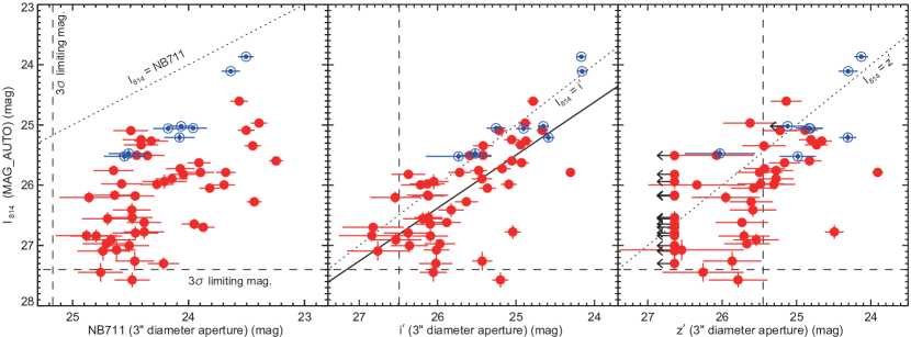
Figure 6.— Distribution of the 62 ACS-detected LAEs in the $I_{814}$–$NB711$ (left), $I_{814}$–$i^{\prime}$ (middle), and $I_{814}$–$z^{\prime}$ planes (right). For the double-component LAEs represented by blue double circles, sum of $I_{814}$ of each component is adopted in this plot. The dotted lines represent the equality of $I_{814}$ and $NB711$, $i^{\prime}$, or $z^{\prime}$. The $3\sigma$ limiting magnitude of ACS in a $1^{\prime\prime}$ diameter aperture, 27.4 mag, is shown by the horizontal dashed line, while those of NB711–, $i^{\prime}$–, and $z^{\prime}$–band images in a $3^{\prime\prime}$ diameter aperture, 25.17, 26.49, and 25.45 mag, are shown by the vertical dashed lines, respectively. In the middle panel, the solid line represents the best-fit linear relation between $I_{814}$ and $i^{\prime}$: $I_{814}=0.88(i^{\prime}-29.0)+29.0$. In the right panel, the LAEs fainter than the $1\sigma$ limiting magnitude of $z^{\prime}$ are located at $z^{\prime}=z^{\prime}(1\sigma)=26.64$ mag with arrows.

The detected emission in the F814W-band filter seems to be primarily from rest-frame UV continuum rather than Ly$\alpha$ line emission. This is clearly exhibited by the presence of a positive correlation between $I_{814}$ and $i^{\prime}$, which are close to $I_{814}\sim i^{\prime}$, as shown in the middle panel of Figure 6. The linear correlation coefficient is estimated to be $r=0.72$. It is similar for $z^{\prime}$, which linear correlation coefficient is $r=0.61$, while dispersion from $I_{814}=z^{\prime}$ relation is more significant. On the other hand, the correlation between $I_{814}$ and $NB711$ appears to be poorer compared with the correlations between $I_{814}$ and $i^{\prime}$ or $z^{\prime}$ (its linear correlation coefficient is $r=0.56$). This result is consistent with the facts that most LAEs have observer-frame EW much smaller than $\Delta\lambda$ of the F814W (i.e., 2511 Å) and that the wavelength of the NB711 band which is almost blue edge of the wavelength coverage of the F814W-band filter (see Figure 1).

Therefore, we can conclude that the ACS F814W-band images primarily probe rest-frame UV continuum emission from young massive stars in the LAEs at $z=4.86$.

3.2. Size: Half-light Radius and Half-light Major Radius

Then we analyze the sizes of our LAE sample in the ACS F814W-band images, that is, half-light radius $R_{\mathrm{HL}}$ and half-light major radius $a_{\mathrm{HL}}$. We emphasize that these measured sizes should be considered as the extent of the young star-forming regions in the LAEs and they do not necessarily reflect the stellar mass distribution since the F814W-band images mainly prove their rest-frame UV continuum emissions at wavelengths of $\sim 1200$–1640 Å as presented in Section 3.1. Note that the measured half-light radii of $\approx 4600$ unsaturated stars with $I_{814}=20$–22 mag and $\mathrm{FWHM}\leq 4~{}\mathrm{pix}$ ($=0\farcs 12$) in the ACS F814W-band images, $R_{\mathrm{PSF}}$, are typically 0$\farcs$07; we adopt this angular scale as the “PSF size” of the ACS F814W-band images in our analysis.

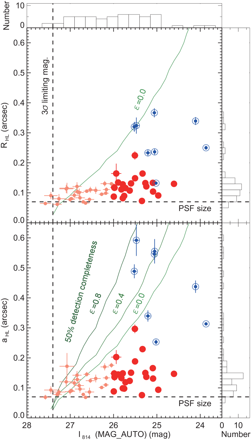
Figure 7.— Distributions of the 54 ACS-detected LAEs in the $R_{\mathrm{HL}}$–$I_{814}$ (top) and $a_{\mathrm{HL}}$–$I_{814}$ (bottom) planes. In the main panels, the LAEs with single- and double-components in the ACS F814W-band images are represented by the red filled and blue double circles, respectively. For the 8 double-component LAEs, the size and magnitude of the double ACS components measured as a single object are plotted. The ACS sources with $I_{814}\geq 26$ mag are shown by the small symbols. The $3\sigma$ limiting magnitude in a $1^{\prime\prime}$ diameter aperture and PSF half-light radius derived from stars, 27.4 mag and 0$\farcs$07, are also shown by the vertical and horizontal dashed lines, respectively. Note that we show the same value of $R_{\mathrm{PSF}}$ both in the top and bottom panels since the PSF is found to have negligibly small ellipticity (i.e., $\epsilon_{\mathrm{PSF}}<0.03$). The solid curves in the bottom panel indicate the 50% detection completenesses for exponential disk objects with the input ellipticities of $\epsilon^{\mathrm{in}}=0.0$, 0.4, and 0.8 estimated by a Monte Carlo simulation. The same curve with $\epsilon^{\mathrm{in}}=0.0$ is also depicted by the solid curve in the top panel. The distributions shown in the main panels are projected onto the two side panels where histograms of $I_{814}$, $R_{\mathrm{HL}}$, and $a_{\mathrm{HL}}$ are displayed.

Figure 7 shows the distributions of the 54 ACS-detected LAEs in the $R_{\mathrm{HL}}$–$I_{814}$ and $a_{\mathrm{HL}}$–$I_{814}$ planes. It is found that the ACS magnitudes $I_{814}$ of the LAEs are widely distributed in 23.87–27.57 mag with the mean value of $\langle I_{814}\rangle=25.99\pm 0.11$ mag. Both sizes of $R_{\mathrm{HL}}$ and $a_{\mathrm{HL}}$ of the LAEs are also found to be widely distributed in $R_{\mathrm{HL}}=0\farcs 06$–0$\farcs$37 and $a_{\mathrm{HL}}=0\farcs 07$–0$\farcs$59 with mean values of $\langle R_{\mathrm{HL}}\rangle=0\farcs 133\pm 0\farcs 010$ and $\langle a_{\mathrm{HL}}\rangle=0\farcs 175\pm 0\farcs 017$. Their distributions are similar with each other, having a concentration at small sizes and an elongated tail toward large sizes. As shown in Figure 7, both distributions of $R_{\mathrm{HL}}$ and $a_{\mathrm{HL}}$ are not concentrated around the means but show a clear separation between the single- and double-component LAEs; the latters have larger sizes than the formers typically. Moreover, all single-component LAEs are found to have sizes of $\lesssim 0\farcs 3$; if the double-component LAEs are excluded, the mean half-light major radius becomes 0$\farcs$13.

Most of the ACS sources have $a_{\mathrm{HL}}>R_{\mathrm{HL}}$, implying that they have non-zero ellipticities. Since $a_{\mathrm{HL}}$ is generally considered to be a more appropriate measure of size than $R_{\mathrm{HL}}$ for such sources having non-zero ellipticities, we adopt $a_{\mathrm{HL}}$ as the fiducial size of the individual ACS source in the following, rather than $R_{\mathrm{HL}}$.

In Figure 7, in order to see the effect of limiting surface brightness in our ACS data, we also plot the 50% detection completeness limits for faint extended sources in the ACS F814W-band images estimated via performing Monte Carlo simulations; the details of our Monte Carlo simulations are described in Appendix A.1. As the resultant 50% detection completeness is found to depend on the input ellipticity $\epsilon^{\mathrm{in}}$, we show the 50% detection completeness limits for $\epsilon^{\mathrm{in}}=0.0$, 0.4, and 0.8 in the bottom panel of Figure 7. This simulation suggests that, in our ACS images, extended objects may suffer from the effect of limiting surface brightness if they have small ellipticities and are fainter than $I_{814}\sim 26$ mag, which is close to the mean magnitude for the ACS sources. There are found to be a non-negligible fraction of the ACS sources (i.e., $9/54=16.7\%$) in the domain where the detection completeness limit for $\epsilon^{\mathrm{in}}=0.0$ is below 50%. Hence, the number fraction of the LAEs having extended ACS sources can be larger than the observed one.

3.3. Ellipticity

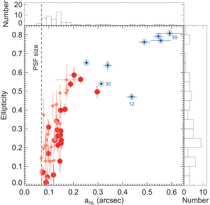
Figure 8.— Distribution of the 54 ACS sources in the $\epsilon$–$a_{\mathrm{HL}}$ plane. The symbols are the same as those in Figure 7. The vertical dashed line indicates the PSF size of the ACS F814W-band images derived from stars. The ID of a double-component LAE which is an outlier in the positive relationship between ellipticity and $a_{\mathrm{HL}}$ (i.e., #12) is labeled for reference. We also label the IDs of two double-component LAEs (i.e., #30 and #59) for reference. The distribution in the main panel is projected onto the two side panels where histograms of $a_{\mathrm{HL}}$ and $\epsilon$ are displayed.

The measured ellipticities of the 54 ACS sources are widely distributed from 0.02 (i.e., almost round-shape) to 0.81 (i.e., elongated- or ellipsoidal-shape) as shown in Figure 8 and Table 3. It is found that the double-component LAEs tend to have larger ellipticities than the single-component LAEs; at $\epsilon>0.6$, all sources are the double-component LAEs.

We also find a strong positive correlation between $\epsilon$ and $a_{\mathrm{HL}}$ as presented in Figure 8 (its Spearman’s rank-order correlation coefficient $\rho$ and Kendall’s $\tau$ are $\rho=0.74$ and $\tau=0.58$, respectively); larger LAEs have more elongated shapes. Moreover, all ACS sources larger than 0$\farcs$2 have elongated morphologies ($\epsilon\gtrsim 0.5$), except for a double-component LAE at $a_{\mathrm{HL}}\sim 0\farcs 44$ and $\epsilon\sim 0.47$ (i.e., the LAE #12 as labeled in Figure 8). In other words, there is no LAE with large size and round shape, that is, $a_{\mathrm{HL}}\gtrsim 0\farcs 2$ and $\epsilon\lesssim 0.45$. It should be emphasized that, since such large round-shaped galaxies can be detected if they are bright enough (i.e., $I_{814}\lesssim 26$ mag) as shown in Figure 7 (see also Figure 18), the absence of such galaxies can be considered as real result, not suffered by selection bias against them.

It is possible that measuring the sizes and ellipticities of the double-component LAEs as single sources makes the correlation strengthen. This is because their sizes and ellipticities are found to be well correlated with the separations between the two components (see Tables 3 and 4) in the sense that the LAE with larger separation has larger size and ellipticity as a system with two components. In the following section, we re-measure the sizes and ellipticities of individual ACS sources in the double-component LAEs separately and re-examine the correlation with size and ellipticity for the resultant quantities.

3.4. Size and Ellipticity of Individual ACS Component and Their Correlation

As described in Section 2, the 8 ACS-detected LAEs are found to consist of the double components with close angular separation (i.e., $\lesssim 1^{\prime\prime}$) in the ACS images. We have shown their morphological properties measured as single systems with double components in the previous Sections 3.2 and 3.3. However, the distributions of single- and double-component LAEs in both size and ellipticity are found to be clearly different from each other; the double-component LAEs have systematically larger sizes and ellipticities than the single-component LAEs as shown in Figure 8. Moreover, as described in the previous section, the sizes and ellipticities of the double-component LAEs are found to be well correlated with the angular separation between the two components. These findings may indicate that, for the 8 double-component LAEs, the morphological properties of individual ACS components should be measured separately so that they might be similar to those of the single-component LAEs.

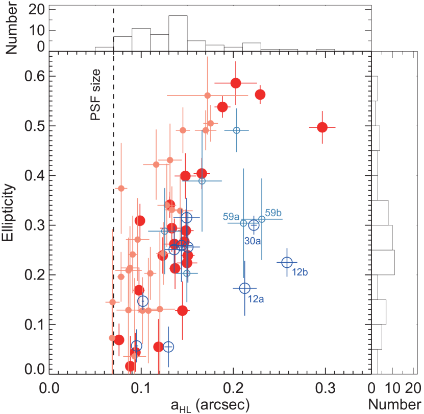
Figure 9.— Same as Figure 8 but for the distribution in which the double ACS components in the 8 double-component LAEs are plotted separately. The components of the single- and double-component LAEs are shown as red filled and blue open circles, respectively. The double-component LAEs with $I_{814}\geq 26$ mag are shown by the small symbols. The IDs of the 5 double-component LAEs which are outliers in the positive relationship between ellipticity and $a_{\mathrm{HL}}$ are labeled for reference.

Table 4ACS F814W-band Properties for the Individual Components in the 8 Double-component LAEs at $z=4.86$ with ACS Data

ID #	$I_{814}$	$a_{\mathrm{HL}}$	$R_{\mathrm{HL}}$	$\epsilon(I_{814})$	$r_{\mathrm{sep}}$
	(mag)	(arcsec)	(arcsec)		(arcsec)
11a	$26.18\pm 0.08$	$0.15\pm 0.01$	$0.13\pm 0.01$	$0.20\pm 0.06$	$0.59\pm 0.01$
11b	$26.37\pm 0.10$	$0.20\pm 0.01$	$0.15\pm 0.01$	$0.49\pm 0.04$	$\cdots$
12a	$25.43\pm 0.07$	$0.21\pm 0.01$	$0.19\pm 0.01$	$0.17\pm 0.06$	$0.47\pm 0.01$
12b	$24.49\pm 0.03$	$0.26\pm 0.01$	$0.23\pm 0.01$	$0.23\pm 0.03$	$\cdots$
19a	$25.86\pm 0.07$	$0.14\pm 0.01$	$0.12\pm 0.01$	$0.25\pm 0.05$	$0.70\pm 0.01$
19b	$25.76\pm 0.07$	$0.15\pm 0.01$	$0.13\pm 0.01$	$0.32\pm 0.04$	$\cdots$
21a	$26.72\pm 0.12$	$0.13\pm 0.02$	$0.11\pm 0.02$	$0.29\pm 0.09$	$0.98\pm 0.01$
21b	$25.32\pm 0.04$	$0.13\pm 0.00$	$0.13\pm 0.00$	$0.06\pm 0.04$	$\cdots$
30a	$24.56\pm 0.02$	$0.22\pm 0.00$	$0.19\pm 0.01$	$0.30\pm 0.02$	$0.36\pm 0.00$
30b	$24.69\pm 0.01$	$0.10\pm 0.00$	$0.09\pm 0.00$	$0.15\pm 0.02$	$\cdots$
37a	$25.94\pm 0.09$	$0.15\pm 0.01$	$0.13\pm 0.01$	$0.26\pm 0.07$	$0.41\pm 0.01$
37b	$25.98\pm 0.10$	$0.14\pm 0.01$	$0.13\pm 0.01$	$0.26\pm 0.07$	$\cdots$
59a	$26.39\pm 0.11$	$0.21\pm 0.02$	$0.18\pm 0.02$	$0.30\pm 0.11$	$0.53\pm 0.01$
59b	$26.08\pm 0.10$	$0.23\pm 0.02$	$0.19\pm 0.02$	$0.31\pm 0.08$	$\cdots$
68a	$25.17\pm 0.02$	$0.09\pm 0.00$	$0.09\pm 0.00$	$0.06\pm 0.03$	$0.97\pm 0.01$
68b	$27.23\pm 0.15$	$0.17\pm 0.02$	$0.13\pm 0.02$	$0.39\pm 0.10$	$\cdots$

Note. — (a) The LAE ID given in Shioya et al. (2009). (b) SExtractor’s MAG_AUTO magnitude and its $1\sigma$ error. (c) Half-light major radius and its $1\sigma$ error measured on ACS F814W-band images. (d) Half-light radius and its $1\sigma$ error measured on ACS F814W-band images. (e) Ellipticity and its $1\sigma$ error measured on ACS F814W-band images. (f) Angular separation between the two components in a double-component LAE and its $1\sigma$ error.

Figure 9 shows the resultant distribution in which, even for the double-component LAEs, both of $\epsilon$ and $a_{\mathrm{HL}}$ of the individual ACS components are measured separately using SExtractor with the same parameters shown in Table 1. The morphological properties for the individual components of the 8 double-component LAEs as well as their angular separations are listed in Table 4. Compared with the distributions shown in Figure 8, the distribution of the double-component LAEs becomes similar to that of the single-component LAEs, while there seem to be five outliers at $a_{\mathrm{HL}}\sim 0\farcs 21$–0$\farcs$26 and $\epsilon\sim 0.17$–0.31; the outliers are the LAEs #12a, #12b, #30a, #59a, and #59b as labeled in Figure 9. As shown in Figure 3 and Table 4, the morphological properties of these outliers may be affected by the other component of a pair because of the close angular separation $r_{\mathrm{sep}}$, which is characterized by $r_{\mathrm{sep}}\lesssim 2.5a_{\mathrm{HL}}$. On the other hand, those of other double-component LAEs are found to be characterized by $r_{\mathrm{sep}}\gtrsim 3a_{\mathrm{HL}}$ and hence they could not be affected by the other component.

Figure 9 also shows that the positive correlation between $\epsilon$ and $a_{\mathrm{HL}}$ still exists, while it becomes weaker ($\rho=0.64$ and $\tau=0.46$) compared with the correlation shown in Figure 8 ($\rho=0.74$ and $\tau=0.58$). If we consider that, as usually do, the LAE consists of thin disk and the ellipticity of ACS source reflects the inclination angle to its disk, the existence of such correlation and the absence of the sources with large $a_{\mathrm{HL}}$ and small $\epsilon$ are unnatural. We will discuss their origin(s) in Section 4.4.

4. DISCUSSION

4.1. Comparison of Size and Ellipticity with Those in The Literatures

As shown in Section 3.2, the single-component LAEs are found to be widely distributed in $a_{\mathrm{HL}}$ of rest-frame UV continuum from 0$\farcs$07 to 0$\farcs$30 ($\langle a_{\mathrm{HL}}\rangle=0\farcs 13$), which correspond to the physical sizes of 0.45 kpc and 1.90 kpc (0.83 kpc for the mean) at $z=4.86$. These measured sizes are quantitatively consistent with the previous measurements for the sizes in rest-frame UV continuum of the LAEs at $z\sim 2$–6 compiled in Malhotra et al. (2012; see also Hagen et al. 2014 for more recent observational results of the size measurements for the LAEs at $z=1.9$–3.6). Therefore, our size measurements for the LAEs at $z=4.86$ provide a further support to the result of Malhotra et al. (2012), that is, the sizes of LAEs in rest-frame UV continuum do not show redshift evolution in $z\sim 2$–6.

In contrast, the sizes of the double-component LAEs are systematically larger than those of the previous measurements; $a_{\mathrm{HL}}$ of the double-component LAEs ranges from 0$\farcs$25 to 0$\farcs$59 with a mean of 0$\farcs$44 (see Figure 8). On the other hand, their sizes are found to be also consistent with those in the literature if their sizes of the individual ACS components are adopted; as shown in Table 4, $a_{\mathrm{HL}}$ of the individual components in the double-component LAEs are in the range of 0$\farcs$09–0$\farcs$26 with a mean of 0$\farcs$17 (see Figure 9). Therefore, it seems to be more natural that the individual ACS components in the double-component LAEs are typical LAEs and that the double-component LAEs are interacting and/or merging galaxies compared to the interpretation that they are sub-components (e.g., star-forming clumps) in an LAE. We will discuss these interpretations of our ACS sources further in Section 4.6.

In terms of $\epsilon$, we also presented in Figure 9 (i.e., the case that the ACS components in the double-component LAEs are treated separately) that the distribution of the ACS sources in $\epsilon$ shows a peak around the mean ellipticity of $\langle\epsilon\rangle=0.27$ and has long tails toward both smaller and larger ellipticities in the range of $\epsilon=0.02$–0.59. This distribution in $\epsilon$ is found to be quite similar to the previous observational estimates for the LAEs at $z\sim 2.2$ (Shibuya et al. 2014) and $z\sim 3.1$ (Gronwall et al. 2011). Although we found the positive correlation between $\epsilon$ and $a_{\mathrm{HL}}$ as shown in Figure 9, such correlation has not been investigated so far; therefore, we do not have any previous results that can be compared with ours. It is still unclear whether or not such correlation is seen among LAEs at different redshifts and how it evolves with redshift. Nevertheless, we will discuss the origin(s) of the positive correlation in Section 4.4.

4.2. Implication for the Sizes of the ACS-undetected LAEs

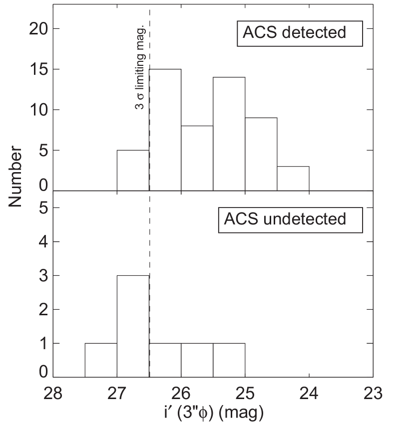
Figure 10.— Frequency distributions of $i^{\prime}$–band magnitudes for the 54 ACS-detected (top) and 7 ACS-undetected LAEs (bottom). The $3\sigma$ limiting magnitude of $i^{\prime}$–band images in a $3^{\prime\prime}$ diameter aperture, 26.49 mag, is also represented by the vertical dashed line.

Among the 61 LAEs with the ACS F814W-band imaging data, 7 LAEs are not detected in the ACS images. Here we try to estimate the half-light radii of these ACS-undetected LAEs using the correlation between $I_{814}$ and $i^{\prime}$ found for the ACS-detected LAEs (see Figure 6) and the $i^{\prime}$–band magnitude distribution of the ACS-undetected LAEs.

As shown in Figure 10, while the ACS-undetected LAEs are found to be at fainter part in the $i^{\prime}$–band magnitude distribution compared with the ACS-detected LAEs, most of the ACS-undetected LAEs have similar $i^{\prime}$–band magnitudes to those of the ACS-detected LAEs. Considering the result of $I_{814}\approx i^{\prime}$ found for the ACS-detected LAEs, the ACS-undetected LAEs with similar $i^{\prime}$–band magnitudes to the ACS-detected LAEs ought to be detected if they are compact and have small $R_{\mathrm{HL}}$. Therefore, the results of their non-detection in the ACS images imply that the surface brightnesses of the 7 ACS-undetected LAEs are too low to be detected; that is, even if they are bright enough to be detected in $I_{814}$, they cannot be detected in ACS image in the case that they are spatially extended significantly as discussed in Section 3.2 (see the 50% detection completeness shown in the top panel of Figure 7). Therefore, large $R_{\mathrm{HL}}$ can be expected for the ACS-undetected LAEs.

We can estimate the half-light radii of the ACS-undetected LAEs as follows. First, we evaluate the expected $I_{814}$-band magnitude from $i^{\prime}$–band magnitude, $I_{814}(i^{\prime})$, using the best-fit linear relation between $I_{814}$- and $i^{\prime}$–band magnitudes for the ACS-detected LAEs: $I_{814}(i^{\prime})=0.88(i^{\prime}-29.0)+29.0$. This is motivated by the result that $I_{814}$ is well correlated with $i^{\prime}$ as described in Section 3.1. Providing $i^{\prime}=25.23$–27.04 mag for the ACS-undetected LAEs, we obtain $I_{814}(i^{\prime})=25.7$–27.3 mag. Then, as the ACS-undetected LAEs are expected to be in the domain on the $R_{\mathrm{HL}}$–$I_{814}$ plane, where detection completeness is low, a lower-limit of $R_{\mathrm{HL}}$ for the ACS-undetected LAEs can be estimated from $I_{814}(i^{\prime})$ and the curve in the $R_{\mathrm{HL}}$–$I_{814}$ plane at which detection completeness for exponential disk objects with the input ellipticity of $\epsilon^{\mathrm{in}}=0.0$ is 50% (see Figure 7). As a result, the expected half-light radii of the ACS-undetected LAEs are $R_{\mathrm{HL}}\gtrsim 0\farcs 07$–0$\farcs$32. This result may imply that there are some LAEs with very large $R_{\mathrm{HL}}$ among the ACS-undetected LAEs.

4.3. Comparison of the Sizes in Ly$\alpha$ and UV Continuum

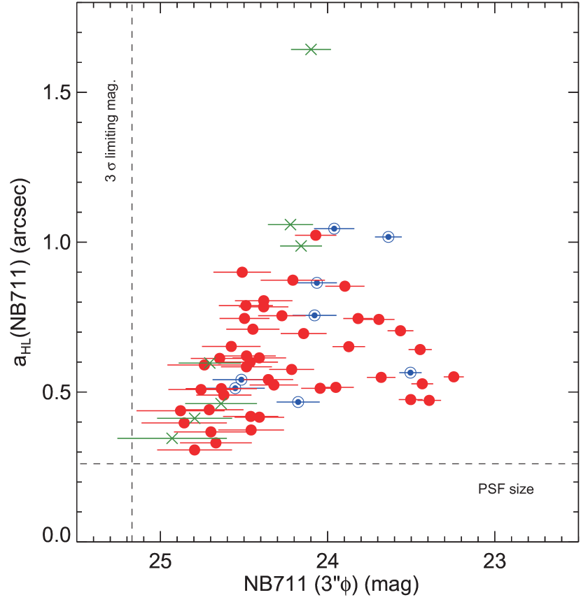
Figure 11.— Distribution of the 60 LAEs with ACS F814W–band imaging data and with measured $a_{\mathrm{HL}}(\mathrm{NB711})$ in the $a_{\mathrm{HL}}(\mathrm{NB711})$–$NB711$ plane. The 7 ACS-undetected LAEs are shown by green crosses and the 45 (8) ACS-detected LAEs with single (double) component(s) are represented by red filled (blue double) circles. The $3\sigma$ limiting magnitude in a $3^{\prime\prime}$ diameter aperture and the PSF half-light radius of NB711–band images, 25.17 mag and 0$\farcs$25, respectively, are also indicated by the vertical dotted and horizontal dashed lines.

In Section 3.2, we found that the ACS-detected LAEs have a wide range of $a_{\mathrm{HL}}$ in the ACS F814W-band images from 0$\farcs$07 to 0$\farcs$59 ($\langle a_{\mathrm{HL}}(\mathrm{F814W})\rangle=0\farcs 175\pm 0\farcs 017$). These angular scales correspond to the physical scales of 0.45–3.8 kpc ($1.11\pm 0.11$ kpc for the mean) at $z=4.86$. As shown in Figure 11, the half-light major radii in the NB711–band images, $a_{\mathrm{HL}}(\mathrm{NB711})$, of the 61 LAEs with ACS data are also found to widely distribute in 0$\farcs$31–1$\farcs$64, corresponding to the physical scales of 1.97–10.45 kpc at $z=4.86$. Since the PSF half-light radius of NB711–band images is 0$\farcs$25, most LAEs are significantly extended in Ly$\alpha$ emissions. This result is consistent with previous studies (e.g., Taniguchi et al. 2005, 2009, 2015; Malhotra et al. 2012; Mawatari et al. 2012; Momose et al. 2014).

It is interesting to examine the relation between $a_{\mathrm{HL}}(\mathrm{NB711})$ and $a_{\mathrm{HL}}(\mathrm{F814W})$ for the ACS-detected LAEs. As shown in Figure 12, $a_{\mathrm{HL}}(\mathrm{NB711})$ is systematically larger than $a_{\mathrm{HL}}(\mathrm{F814W})$ except for three double-component LAEs with $a_{\mathrm{HL}}(\mathrm{NB711})/a_{\mathrm{HL}}(\mathrm{F814W})\approx 1$ (i.e., the LAEs #11, #19, and #59 have the ratios of 1.04, 0.85, and 0.96, respectively). The ratio of $a_{\mathrm{HL}}\mathrm{(NB711)}/a_{\mathrm{HL}}(\mathrm{F814W})$ is widely distributed from $\approx 1$ to $\approx 10$. This result may be a consequence of the non-detection of extended UV continuum in the ACS images since extended sources are difficult to be detected as discussed in Section 3.2. Nevertheless, the large ratio of $a_{\mathrm{HL}}\mathrm{(NB711)}/a_{\mathrm{HL}}(\mathrm{F814W})$ can be a real feature for high-$z$ LAEs. In this case, it is suggested that the compact star-forming regions in the LAEs (i.e., $\lesssim 0\farcs 30$ or $\lesssim 1.9$ kpc) observed by the ACS F814W-band images ionize the surrounding gas, which emits spatially extended Ly$\alpha$ (i.e., $\gtrsim 0\farcs 3$ or $\gtrsim 1.9$ kpc) detected in the NB711-band images.

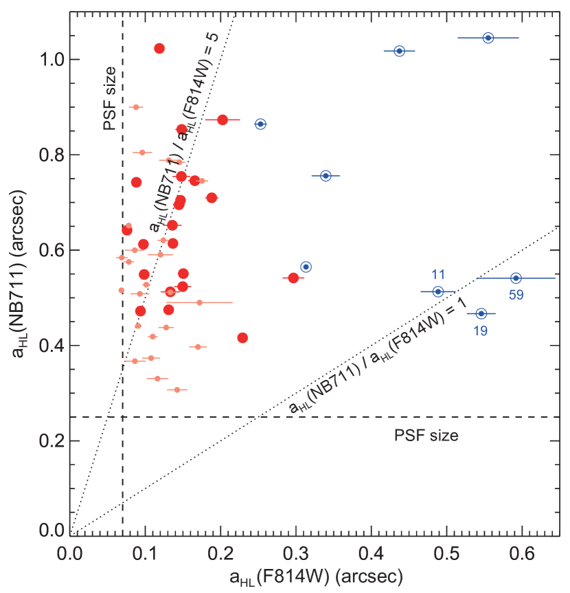
Figure 12.— Distribution of the 53 ACS sources with measured $a_{\mathrm{HL}}(\mathrm{NB711})$ in the $a_{\mathrm{HL}}\mathrm{(NB711)}$–$a_{\mathrm{HL}}\mathrm{(F814W)}$ plane. Symbols are the same as those in Figure 8. The PSF sizes of ACS F814W– and NB711–band images are presented by vertical and horizontal dashed lines, respectively. The dotted lines represent $a_{\mathrm{HL}}\mathrm{(NB711)}/a_{\mathrm{HL}}\mathrm{(F814W)}=1$ (lower) and 5 (upper) as labeled. The IDs of the 3 outliers located at $a_{\mathrm{HL}}(\mathrm{NB711})/a_{\mathrm{HL}}(\mathrm{F814W})\approx 1$ are also labeled for reference.

4.4. Origin of the Correlation between Ellipticity and Size

As described in Section 3.3, the ACS sources show a strong positive correlation between ellipticity $\epsilon$ and half-light major radius $a_{\mathrm{HL}}$, that is, larger ACS sources have more elongated morphologies (Figure 8). As shown in Section 3.4 and Figure 9, while the correlation is found to be strengthened by our measurements of $\epsilon$ and $a_{\mathrm{HL}}$ for the two ACS sources in individual double-component LAEs collectively, the correlation still exists if $\epsilon$ and $a_{\mathrm{HL}}$ are measured for the two ACS sources in double-component LAEs separately.

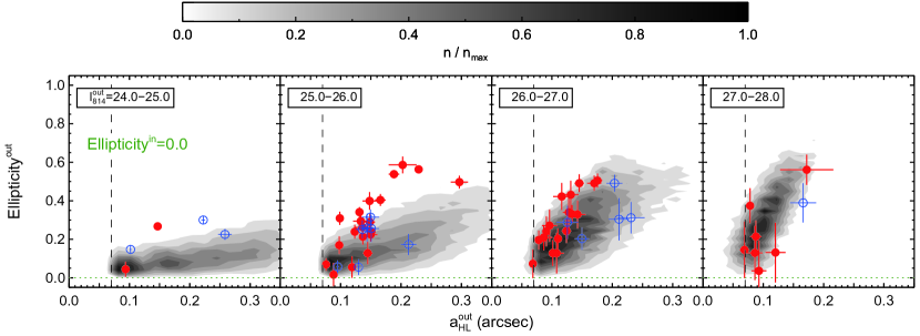
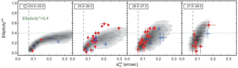
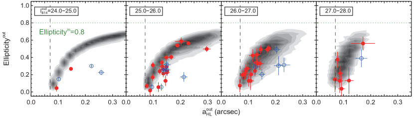
Figure 13.— Distributions of the artificial sources in the $\epsilon$–$a_{\mathrm{HL}}$ plane. 1000 artificial sources with the exponential light profile, each of which is assumed to consist of a single component, are generated by a Monte Carlo simulation and prepared for each set of input parameters, that is, $I_{814}^{\mathrm{in}}=24.0$–28.0 mag, $a_{\mathrm{HL}}^{\mathrm{in}}=0\farcs 03$–0$\farcs$36, and $\epsilon^{\mathrm{in}}=0.0$–0.9 (see Appendix A.1 for details). The resultant distributions are plotted separately for the artificial sources with the input ellipticities $\epsilon^{\mathrm{in}}$ of 0.0 (top), 0.4 (middle), and 0.8 (bottom), as well as those with the output magnitudes $I_{814}^{\mathrm{out}}$ as labeled in each panel. The grayscale represents the number of the artificial sources in the linear scale from 0 (white) to $n_{\mathrm{max}}$ (black), where $n_{\mathrm{max}}$ is the maximum number of the artificial sources in a grid and different among panels. Note that these grayscales are evaluated only from the detected artificial sources. The vertical dashed lines indicate the PSF half-light radius $R_{\mathrm{PSF}}$ and the horizontal dotted lines represent $\epsilon^{\mathrm{in}}$. The observed 62 ACS sources are overlaid with the same symbols as those in Figure 9.

Here, we examine the possibilities that the observed correlation between $\epsilon$ and $a_{\mathrm{HL}}$ is (1) an “apparent” correlation caused by deformation effects for a single source (e.g., pixelization, PSF broadening, and shot noise) and (2) the “intrinsic” correlation originated from blending with unresolved double or multiple sources through Monte Carlo simulations. We consider the correlation between $\epsilon$ and $a_{\mathrm{HL}}$ for the individual ACS sources of the double-component LAEs (i.e., the correlation shown in Figure 9) since it is more natural interpretation as described in Section 3.4.

4.4.1 Apparent Correlation Caused by Deformation Effects

As shown in the previous section, our ACS sources are typically very compact and faint. In general, the sizes and ellipticities of compact sources whose angular scales are comparable to the pixel scale can be modified because of the pixelization of the digital images depending on their places on the pixels. However, since the ACS images we used have sufficiently large PSF half-light radius of $R_{\mathrm{PSF}}=0\farcs 07$ compared to the pixel scale of 0$\farcs$03, such pixelization seems not to affect the morphological parameters of the detected sources, which are definitely affected by PSF broadening. The sizes and ellipticities of faint sources whose surface brightnesses are comparable to the surface brightness limit of imaging data also tend to be modified by shot noise; that is, if a bright pixel contaminated by shot noise appears near a compact faint source, they could be blended with each other and detected as a single elongated source via our source detection using SExtractor. The angular separation between the noise-contaminated pixel and source is translated into the size and ellipticity of the detected source. Therefore, a positive correlation between $\epsilon$ and $a_{\mathrm{HL}}$ is naturally expected to emerge even if source has intrinsically compact and perfectly round shape.

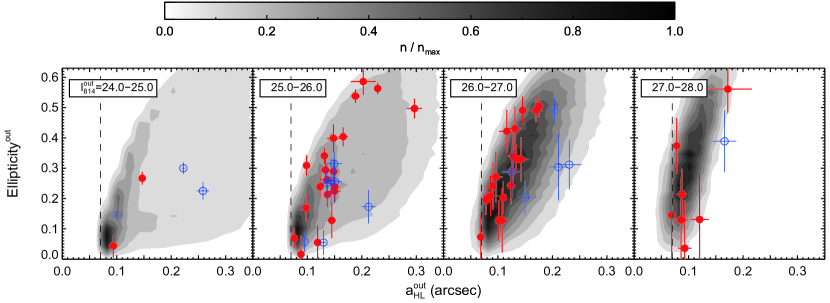
Figure 14.— Same as Figure 13, but for the result of a Monte Carlo simulation for the artificial sources with various $\epsilon^{\mathrm{in}}$ uniformly distributed in 0.0–0.9.

In order to examine these deformation effects from PSF broadening and shot noise on the distribution in the $\epsilon$–$a_{\mathrm{HL}}$ plane, we perform the Monte Carlo simulation which is the same as the one done to estimate the detection completeness (see Appendix A.1 for the details). Figure 13 shows the resultant distributions of the detected artificial sources with $\epsilon^{\mathrm{in}}=0.0$ (top), 0.4 (middle), and 0.8 (bottom) in the $\epsilon^{\mathrm{out}}$–$a_{\mathrm{HL}}^{\mathrm{out}}$ plane. As expected, the deformation effects are found to produce a correlation between $\epsilon$ and $a_{\mathrm{HL}}$ which is similar to the observed correlation, although the sources intrinsically distribute in the $\epsilon^{\mathrm{in}}$–$a_{\mathrm{HL}}^{\mathrm{in}}$ plane uniformly.

How do these deformation effects produce such an apparent correlation between $\epsilon$ and $a_{\mathrm{HL}}$? The PSF broadening significantly affects the shapes of the detected sources with small sizes, in the sense that their measured ellipticities $\epsilon^{\mathrm{out}}$ converge on the PSF ellipticity, $\epsilon_{\mathrm{PSF}}\approx 0$, regardless of $I_{814}^{\mathrm{in}}$ and $\epsilon^{\mathrm{in}}$ of them. Since this effect becomes less important for larger sources with sufficiently bright surface brightnesses, their $\epsilon^{\mathrm{out}}$ are expected to be reproduced as $\epsilon^{\mathrm{out}}\sim\epsilon^{\mathrm{in}}$. Therefore, if the sources have non-zero $\epsilon^{\mathrm{in}}$, a correlation between $\epsilon^{\mathrm{out}}$ and $a_{\mathrm{HL}}^{\mathrm{out}}$ emerges, as shown in the two left-most panels for $\epsilon^{\mathrm{in}}=0.4$ and 0.8 of Figure 13. On the other hand, the effects of shot noise can be easily seen in the apparent positive correlation between $\epsilon^{\mathrm{out}}$ and $a_{\mathrm{HL}}^{\mathrm{out}}$ for the sources with $\epsilon^{\mathrm{in}}=0.0$; the ellipticities of the detected sources increase with $a_{\mathrm{HL}}^{\mathrm{out}}$ although their input ellipticities are exactly zero. The emergence of the correlation can be interpreted via a combination of lower detection completenesses and larger influences of noise-contaminated pixel for the sources with lower surface brightnesses, that is, those with larger sizes and/or smaller ellipticities (see Figure 18). These effects are more significant for the sources with fainter magnitudes of $I_{814}^{\mathrm{out}}$ and hence the slopes of the correlation become steeper for fainter sources. For the sources with $I_{814}^{\mathrm{out}}>26$ mag, since the effects of shot noise are dominant, the correlation does not depend on $\epsilon^{\mathrm{in}}$ significantly as shown in the two right-most panels of Figure 13.

As a combination of these deformation effects, the detected artificial sources distribute similar to the observed distribution in the $\epsilon^{\mathrm{out}}$–$a_{\mathrm{HL}}^{\mathrm{out}}$ plane as shown in Figure 14, although they are uniformly distributed in the $\epsilon^{\mathrm{in}}$–$a_{\mathrm{HL}}^{\mathrm{in}}$ plane. This result may indicate that the observed correlation between $\epsilon$ and $a_{\mathrm{HL}}$ is apparent one caused by the deformation effects. The dispersion of $\epsilon^{\mathrm{out}}$ for a given $a_{\mathrm{HL}}^{\mathrm{out}}$ is predicted to be larger for the sources with bright magnitudes of $I_{814}^{\mathrm{out}}$. This is because the distributions of the brighter sources in the $\epsilon^{\mathrm{out}}$–$a_{\mathrm{HL}}^{\mathrm{out}}$ plane do depend on $\epsilon^{\mathrm{in}}$ and those of the fainter sources do not. Our simulation suggests that, in order to reproduce the distributions of the LAEs with relatively bright (i.e., $I_{814}\approx 25$–26 mag) and large sizes and ellipticities (i.e., $a_{\mathrm{HL}}\approx 0\farcs 20$ and $\epsilon\approx 0.45$), intrinsically large ellipticities (i.e., $\epsilon^{\mathrm{in}}\gtrsim 0.8$) are required. We note that the observed distribution can be reproduced even better if the artificial sources have a Gaussian distribution peaked at $(a_{\mathrm{HL}}^{\mathrm{in}},\ \epsilon^{\mathrm{in}})\sim(0\farcs 15,\ 0.3)$.

4.4.2 Intrinsic Correlation Originated from Blending with Unresolved Double/Multiple Sources

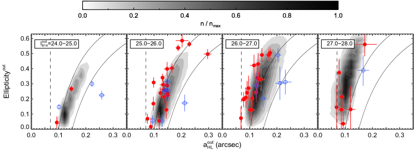
Figure 15.— Same as Figure 13, but for the results of a Monte Carlo simulation in the case that a pair of two identical objects is detected as a single-blended source. 5000 sources which consists of two identical objects with $a_{\mathrm{HL}}^{\mathrm{in}}=0\farcs 07$ and $\epsilon^{\mathrm{in}}=0.0$ are generated in each set of input parameters, that is, $I_{814}^{\mathrm{in}}=25.5$–28.0 mag ($\Delta I_{814}^{\mathrm{in}}=0.5$ mag) and angular separation of 0$\farcs$03–0$\farcs$30 ($\Delta r_{\mathrm{sep}}=0\farcs 03$). Note that the grayscales are evaluated only from the artificial sources detected as single sources (i.e., the sources detected as double detached sources are neglected). The solid curves show the expected correlation between $\epsilon^{\mathrm{out}}$ and $a_{\mathrm{HL}}^{\mathrm{out}}$ through the separation between two identical objects $r_{\mathrm{sep}}$, which is represented as Equations (1) and (2), with $a_{\mathrm{HL}}^{\mathrm{in}}=0\farcs 10$ (left) and 0$\farcs$15 (right).

Another possible origin of the positive correlation between $\epsilon$ and $a_{\mathrm{HL}}$ is blending with unresolved double or multiple sources. Let us consider a simplified situation where two identical round-shaped objects with half-light radius of $a_{\mathrm{HL}}^{\mathrm{in}}$ are located closely with a separation of $r_{\mathrm{sep}}$. If these objects are blended as a single elongated source because of their small angular separation (i.e., $r_{\mathrm{sep}}\lesssim 2a_{\mathrm{HL}}^{\mathrm{in}}$), its half-light major radius of $a_{\mathrm{HL}}^{\mathrm{out}}$ and ellipticity of $\epsilon^{\mathrm{out}}$ can be roughly parameterized with $a_{\mathrm{HL}}^{\mathrm{in}}$ and $r_{\mathrm{sep}}$ as

$$a_{\mathrm{HL}}^{\mathrm{out}} \approx \left(r_{\mathrm{sep}}+2a_{\mathrm{HL}}^{\mathrm{in}}\right)/2,$$ (1)

$$\epsilon^{\mathrm{out}} \approx r_{\mathrm{sep}}/\left(r_{\mathrm{sep}}+2a_{\mathrm{HL}}^{\mathrm{in}}\right).$$ (2)

Since both $a_{\mathrm{HL}}^{\mathrm{out}}$ and $\epsilon^{\mathrm{out}}$ are found to increase with $r_{\mathrm{sep}}$, a positive correlation between these two quantities will emerge even though each component has a perfectly round shape. Under this interpretation, the observed correlation contains useful information that the LAEs may consist of two or more components with small angular separation. In this case, the correlation can be considered as an intrinsic one not an apparent one described in the previous subsection.

In order to examine whether this interpretation results in a similar distribution in the $\epsilon$–$a_{\mathrm{HL}}$ plane to the observed one quantitatively, we perform Monte Carlo simulations whose details are described in Section A.2. The resultant distribution of the artificial sources in the $\epsilon^{\mathrm{out}}$–$a_{\mathrm{HL}}^{\mathrm{out}}$ plane are shown in Figure 15. Since the distributions for the sources with $I_{814}^{\mathrm{out}}>26$ mag are completely determined by the effects of shot noise, the distributions for the double-component sources with $I_{814}^{\mathrm{out}}>26$ mag are similar to those for the single-component sources with $I_{814}^{\mathrm{out}}>26$ mag shown in Figures 13 and 14. On the other hand, the distributions for the double-component sources with $I_{814}^{\mathrm{out}}<26$ mag are different from those for the single-component sources. And these distributions appear to be consistent with the expected distributions from the simplified situation shown by the solid curves in Figure 15. While the observed distribution of the LAEs with $I_{814}<26$ mag is reproduced well, the LAEs with relatively bright (i.e., $I_{814}\approx 25$–26 mag) and large sizes and ellipticities (i.e., $a_{\mathrm{HL}}\approx 0\farcs 20$ and $\epsilon\approx 0.45$) are failed to be reproduced. This is because $\epsilon^{\mathrm{out}}$ cannot be much larger than 0.5 via such a blending of two identical sources since the angular separation should be smaller than $\sim 2a_{\mathrm{HL}}^{\mathrm{in}}$ in order to be detected as a single-blended source. However, these LAEs may also be reproduced if non-zero intrinsic ellipticities are adopted. Moreover, the observed distribution of the LAEs are reproduced even better if the artificial sources with $\epsilon^{\mathrm{in}}=0$ have a Gaussian distribution peaked at $(a_{\mathrm{HL}}^{\mathrm{in}},\ r_{\mathrm{sep}})\sim(0\farcs 10,\ 0\farcs 15)$.

We note that, in our simulation, only the artificial sources with large separation (i.e., $\gtrsim 0\farcs 3$) are well resolved into two detached sources. This result explain the observed results that the double-component LAEs have angular separation of $r_{\mathrm{sep}}>0\farcs 36$ as shown in Table 4 and that the single-component LAEs have $a_{\mathrm{HL}}<0\farcs 3$. In this interpretation, some of the 46 single-component LAEs may contain double or multiple components with close angular separations. Moreover, some of the components in the 8 double-component LAEs can be further resolved into compact components; that is, they can be regarded as multiple-component LAEs which consists of three or more components. Therefore, the double-component fraction in our sample could be as high as $\approx 100$%.

4.5. Dependence of Ly$\alpha$ Line EW and Luminosity on Size

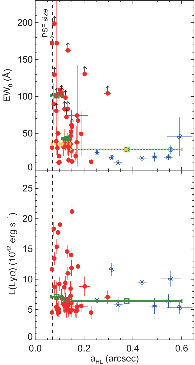
Figure 16.— Distribution in the $\mathrm{EW_{0}}$–$a_{\mathrm{HL}}$ (top) and $L(\mathrm{Ly\alpha})$–$a_{\mathrm{HL}}$ planes (bottom). The filled circles with upward arrows in the top panel indicate the lower limit of $\mathrm{EW_{0}}$. The vertical dashed line indicates the PSF size of ACS image of 0$\farcs$11. The boxes with error bars represent the median values of $\mathrm{EW_{0}}$ (top) and $L(\mathrm{Ly\alpha})$ (bottom) for the ACS counterparts in each bin of $a_{\mathrm{HL}}$, in which the same number of the counterparts enters. For the LAEs with lower limit of $\mathrm{EW_{0}}$, we use their $\mathrm{EW_{0}}$ lower-limit values to evaluate the median values. On the other hand, the crosses with error bars in the top panel show the median values of $\mathrm{EW_{0}}$ for the case that the LAEs with lower limit of $\mathrm{EW_{0}}$ are neglected.

It has been reported observationally that the high-$z$ LAEs and LBGs exhibit anti-correlation between size measured in rest-frame UV continuum and rest-frame Ly$\alpha$ EW, that is, the galaxies with large $\mathrm{EW_{0}}$ tend to have smaller sizes (e.g., Law et al. 2012; Vanzella et al. 2009; Pentericci et al. 2010; Shibuya et al. 2014; see also Bond et al. 2012 against these results). As shown in the top panel of Figure 16, our LAE sample at $z=4.86$ also present such anti-correlation between $\mathrm{EW_{0}}$ and $a_{\mathrm{HL}}$. However, this result seems to depend on the treatment of the LAEs with lower limits of $\mathrm{EW_{0}}$. If they are included to calculate the binned-median values of $\mathrm{EW_{0}}$ using their lower limits of $\mathrm{EW_{0}}$, the anti-correlation between $\mathrm{EW_{0}}$ and $a_{\mathrm{HL}}$ is clearly seen as shown by the boxes with error-bars in the top panel of Figure 16. On the other hand, if they are completely neglected to calculate the robustly determined binned-median values, the anti-correlation disappears. Therefore, in order to conclude whether or not the anti-correlation between $\mathrm{EW_{0}}$ and $a_{\mathrm{HL}}$ does exist, a deeper imaging data of the broadband which is used to determine $\mathrm{EW_{0}}$ (i.e., Subaru $z^{\prime}$ band for our LAE sample) is required. Our LAE sample does not show strong correlation between $L(\mathrm{Ly\alpha})$ and $a_{\mathrm{HL}}$ as shown in the bottom panel of Figure 16, while the dynamic range of $L(\mathrm{Ly\alpha})$ is only a factor of $\sim 5$ and the maximum $L(\mathrm{Ly\alpha})$ seems to decrease as $a_{\mathrm{HL}}$ increases.

Shibuya et al. (2014) found that, for their sample of the LAEs at $z\sim 2.2$, merger fraction decreases at large $\mathrm{EW_{0}}$. If we consider the double-component LAEs as merging galaxies, as discussed in Section 4.6, the same trend is also seen in our sample as shown in Figure 16; all double-component LAEs have $\mathrm{EW_{0}}<50$ Å. Same trend hold for $L(\mathrm{Ly\alpha})$. However, as presented in Section 4.4, we cannot rule out the possibility that the single-component LAEs are merging galaxies. We note that, although the trend seen in the $\mathrm{EW_{0}}$–$a_{\mathrm{HL}}$ plane has been usually interpreted as the absence of the galaxies with large stellar mass (i.e., large in size) and large $\mathrm{EW_{0}}$, the trend is consistent with the model in which the galaxy merger and/or close encounter will activate Ly$\alpha$ emission. This is because the single-component LAEs can contain the galaxies with much smaller separations than the double-component LAEs and because galaxy pairs with smaller separations can result in more enhanced star formation as found in the nearby universe using the Sloan Digital Sky Survey (Patton et al. 2013). Moreover, based on this scenario, since the single-component LAEs can contain both of the galaxies with short and long elapsed times from galaxy merger/interaction which activates Ly$\alpha$ emission, the median values of $\mathrm{EW_{0}}$ and $L(\mathrm{Ly\alpha})$ may not depend on the separation. This expectation is also consistent with the observed distributions of the LAEs shown in Figure 16.

4.6. Implication for Star Formation in the LAEs at $z=4.86$

We detected 54 counterparts in the ACS images for our LAEs at $z=4.86$ in the COSMOS field. While 8 of them have double component with the angular separations of 0$\farcs$36–0$\farcs$98 (i.e., 2.3–6.2 kpc at $z=4.86$), the magnitudes and morphologies of individual components were found to be similar to those of the other 46 single-component LAEs (see Figure 9 and Tables 3 and 4) and the typical LAEs in the literature (e.g., Malhotra et al. 2012; Hagen et al. 2014). This result indicates that the double-component LAEs are interacting and/or merging galaxies with close separation, that is, the projected separation is comparable to or not larger than ten times of the size of a galaxy, $r_{\mathrm{sep}}/a_{\mathrm{HL}}\sim 1$–10.

Moreover, as shown in Section 4.4 through our Monte Carlo simulations, the observed positive correlation between $\epsilon$ and $a_{\mathrm{HL}}$ for our ACS-detected LAEs may indicate that both of the single-component LAEs and the individual components in the double-component LAEs consist of unresolved components with close separation of $r_{\mathrm{sep}}\lesssim 0\farcs 3$ (i.e., $\lesssim 1.9$ kpc at $z=4.86$), while another interpretation for the observed correlation (e.g., apparent correlation caused by the deformation effects such as PSF broadening and shot noise) was still possible. Our Monte Carlo simulation also indicates that a typical size of individual component is $\sim 0\farcs 10$–0$\farcs$15 (i.e., $\sim 0.64$–0.96 kpc at $z=4.86$). Since the observed wavelength of the ACS F814W-band corresponds to rest-frame UV wavelength of $\sim 1200$–1640 Å at $z=4.86$, the ACS components are considered to be young star-forming regions. Therefore, the small separation suggests the following two cases: (1) the individual component is a large star-forming region in an extended galaxy and star-formation activity in the LAEs occurs in a clumpy fashion or (2) individual component in an ACS source is a compact star-forming galaxy and the LAEs are the galaxies in close encounter and/or merger. In order to distinct the above two interpretations, deeper imaging data at longer wavelength with similar or higher spatial-resolution than our ACS F814W-band data is inevitable. If diffuse and faint underlying component which is surrounding the two (or multiple) components is detected and it does not show any signatures of galaxy interaction/merger, the clumpy star-formation in a galaxy will be confirmed.

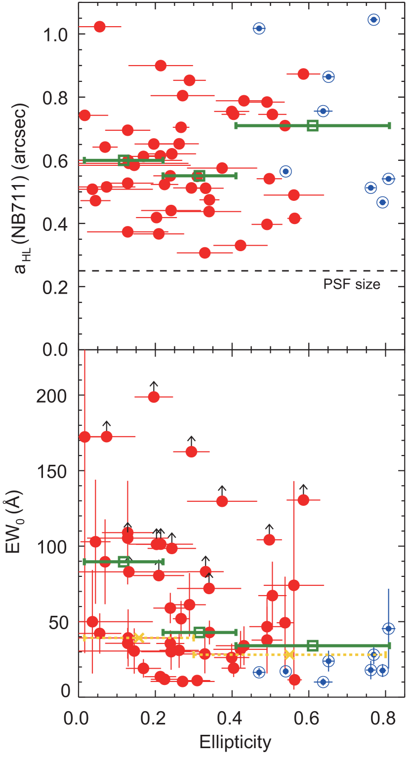
Figure 17.— Same as Figure 16, but for distribution in the $a_{\mathrm{HL}}(\mathrm{NB711})$–$\epsilon$ (top) and $\mathrm{EW_{0}}$–$\epsilon$ planes (bottom). The horizontal dotted line in the top panel indicates the PSF size of NB711–band image of 0$\farcs$25.

In the interpretation of clumpy star-formation in a disk-like galaxy, as usually observed in high-$z$ galaxies (e.g., Elmegreen et al. 2009; Förster Schreiber et al. 2011; Murata et al. 2014; Tadaki et al. 2014), the ellipticity of a source may be an intrinsic property related to the viewing angle of the disk. That is, large ellipticity implies that its viewing angle is close to edge-on and that stellar disk lies in the elongated direction. If we consider that Ly$\alpha$ is emitted in directions perpendicular to the disk, as predicted by the recent theoretical studies for Ly$\alpha$ line transfer (e.g., Verhamme et al. 2012; Yajima et al. 2012b), the pitch angle of Ly$\alpha$ emission will be at right angles to that of UV continuum. Moreover, in such case, it is also expected that the size in Ly$\alpha$ emission $a_{\mathrm{HL}}(\mathrm{NB711})$ shows a positive correlation with ellipticity measured in rest-frame UV continuum because Ly$\alpha$ emitting region in bipolar directions perpendicular to the disk can be viewed in longer distance if the viewing angle of the disk is closer to edge-on, that is, larger ellipticity. However, as presented in the top panel of Figure 17, we do not find such positive correlation between $a_{\mathrm{HL}}(\mathrm{NB711})$ and ellipticity for the 54 ACS-detected LAEs. Furthermore, as shown in the bottom panel of Figure 17, the observed distribution of the LAEs in the $\mathrm{EW_{0}}$–$\epsilon$ plane seems not to be quantitatively consistent with the interpretation of clumpy star-formation in a disk-like galaxy, where $\mathrm{EW_{0}}$ is expected to decrease significantly toward edge-on direction (i.e., larger ellipticity) via radiative transfer effects for Ly$\alpha$ resonance photons (e.g., Verhamme et al. 2012; Yajima et al. 2012b); this result is consistent with Shibuya et al. (2014). Therefore, the interpretation of clumpy star-formation in a disk-like galaxy seems not to be preferred for our LAE sample. This conclusion can be reinforced with the absence of the ACS source with large size and round shape; if there are multiple clumpy star-forming regions in a disk-like galaxy, some of such galaxies will be viewed from face-on, resulting in large size and round shape. We emphasize again that this result is not affected by a selection bias against them if they are bright enough (i.e., $I_{814}\lesssim 26$ mag) as shown in Figures 7 and 18.

On the other hand, the interpretation of merger and/or interaction is broadly consistent with these observed results. The correlation between $\epsilon$ and $a_{\mathrm{HL}}$ can be reproduced by blending with double (or multiple) sources with close separations as shown in Section 4.4.2 through our Monte Carlo simulations. The anti-correlation between the maximum value of $\mathrm{EW_{0}}$ or $L(\mathrm{Ly\alpha})$ and $a_{\mathrm{HL}}$ is also expected if the single-component LAEs are the merging and/or interacting galaxies with close separations and if Ly$\alpha$ emissions are activated in such situation as described in Section 4.5. Moreover, the observed results that the median values of $\mathrm{EW_{0}}$ and $L(\mathrm{Ly\alpha})$ do not depend on $a_{\mathrm{HL}}$ are also consistent with this merger interpretation as shown in Section 4.5. Therefore, the interpretation of merging and/or interacting galaxies seems to be more feasible for our LAE samples.

5. CONCLUSIONS

We have examined the morphological properties of 61 LAEs at $z=4.86$ based on the HST/ACS imaging in the F814W-band filter, which are originally selected in the COSMOS field by S09. Our main results and conclusions are summarized below.

1. While the ACS counterparts of 7 LAEs are not detected, 62 ACS sources are detected with $I_{814}\lesssim 28$ mag for the remaining 54 LAEs. Of the 54 LAEs with ACS sources, 8 LAEs have double ACS components and 46 LAEs have single component.

2. For the double-component 8 LAEs, the angular separation between two components are found to be 0$\farcs$36–0$\farcs$98 ($=2.3$–6.2 kpc at $z=4.86$) with a mean separation of 0$\farcs$63 ($=4.0$ kpc). The angular separation is sufficiently large compared to the PSF size of ACS image, $R_{\mathrm{PSF}}=0\farcs 07$, which is the reason why they are separately detected.

3. Comparing ACS F814W-band magnitude $I_{814}$ with Suprime-Cam NB711–, $i^{\prime}$–, and $z^{\prime}$–band magnitudes, we find that the ACS F814W-band image probes rest-frame UV continuum rather than Ly$\alpha$ line (Figure 6). We observe the extent of star-forming regions in our LAE sample at $z=4.86$ via the F814W-band filter.

4. All of 62 ACS sources have small spatial sizes of $a_{\mathrm{HL}}\sim 0\farcs 07$–0$\farcs$30 ($=0.45$–1.9 kpc) as shown in Figure 9. Their mean size is 0$\farcs$14 ($=0.89$ kpc), which is consistent with the previous measurements for the size in rest-frame UV continuum of the LAEs at $z\sim 2$–6 in the literatures.

5. The measured ellipticities of the 62 ACS sources are widely distributed in $\epsilon=0.02$–0.59 and a positive correlation between $\epsilon$ and $a_{\mathrm{HL}}$ (Figure 9). It is evident even if we exclude the faint ACS sources with $I_{814}>26$ mag. Moreover, the absence of the large (i.e., $a_{\mathrm{HL}}\gtrsim 0\farcs 2$) sources with almost round shape (i.e., $\epsilon\lesssim 0.2$) is also found.

6. The 7 ACS-undetected LAEs are expected to have low surface brightnesses so that they are undetected in our ACS images. We estimate their half-light radii from Suprime-Cam $i^{\prime}$–band magnitudes of $i^{\prime}=25.23$–27.04 mag (Figure 10) to be $R_{\mathrm{HL}}\gtrsim 0\farcs 07$–0$\farcs$32.

7. All ACS sources have significantly smaller sizes in UV continuum than those in Ly$\alpha$ lines probed by NB711–band (Figure 12). The size ratios of $a_{\mathrm{HL}}(\mathrm{NB711})/a_{\mathrm{HL}}(\mathrm{F814W})$ are widely distributed in the range of $\approx 1$–10.

8. The observed positive correlation between $\epsilon$ and $a_{\mathrm{HL}}$ can be interpreted by either (1) an apparent one caused by the deformation effects such as the PSF broadening and shot noise or (2) an intrinsic one originated from blending with unresolved double or multiple sources. These are proved through our Monte Carlo simulations, which reproduce the observed correlations as presented in Figures 14 and 15 for the former and latter interpretations, respectively.

9. Both Ly$\alpha$ EW and luminosity of LAEs do not show strong dependencies on sizes in rest-frame UV continuum (Figure 16). Moreover, there are no LAEs with double ACS components at large $\mathrm{EW_{0}}$ and $L(\mathrm{Ly\alpha})$. These results are consistent with the model in which galaxy merger and/or close encounter will activate Ly$\alpha$ emissions.

10. The 8 double-component LAEs are considered to be merger and/or interacting galaxies since the angular separations between components are significantly larger than the sizes of each component although we cannot completely reject the possibility that their underlying (disk) component is missed by its faintness and they are single object with multiple star-forming knot. The absence of the ACS sources with large sizes and small ellipticities (Figures 8 and 9), the anti-correlation between $\mathrm{EW_{0}}$ or $L(\mathrm{Ly\alpha})$ and $a_{\mathrm{HL}}$ (Figure 16), and the absence of the correlation between $\epsilon$ and $a_{\mathrm{HL}}(\mathrm{NB711})$ (Figure 17) suggest the possibility that a significant fraction of 46 single-component LAEs are also merger/interacting galaxies with a very small separation. In order to decipher which interpretation is adequate for our LAE sample, further observation with high angular resolution at the wavelengths which are longer than the Balmer/4000 Å break in rest frame (i.e., $\gtrsim 2.3~{}\mu$m in observer frame for our LAE sample at $z=4.86$) will be required.

Appendix A Monte Carlo Simulation

In this Appendix, we describe the details of the settings and procedures of our Monte Carlo simulations.

A.1. Single Component

In order to estimate the detection completeness (Section 3.2) and the deformation effects in shape via the PSF broadening and shot noise for faint single sources (Section 4.4.1), we performed the following Monte Carlo simulations. For each artificial ACS F814W-band source, the exponential light profile is adopted, motivated by the observational result that the 47 ACS-detected LAEs at $z=5.7$ in the COSMOS field have the Sérsic index of $n=0.7\pm 0.3$ (Taniguchi et al. 2009). For each set of the given input parameters of $I_{814}^{\mathrm{in}}$, $a_{\mathrm{HL}}^{\mathrm{in}}$, and $\epsilon^{\mathrm{in}}$, we prepare 1000 artificial sources by using the GALFIT software (Peng et al. 2002, 2010). The full ranges (steps) of these input parameters are $I_{814}^{\mathrm{in}}=24.0$–28.0 mag ($\Delta I_{814}^{\mathrm{in}}=0.5$ mag), $a_{\mathrm{HL}}^{\mathrm{in}}=0\farcs 03$–0$\farcs$75 ($\Delta a_{\mathrm{HL}}^{\mathrm{in}}=0\farcs 03$), and $\epsilon^{\mathrm{in}}=0.0$–0.9 ($\Delta\epsilon^{\mathrm{in}}=0.1$); in total, we prepare 2,250,000 artificial sources. We put them into the observed ACS image randomly, convolving them with the PSF image. The photon noises and the Galactic dust extinction (i.e., $A_{\mathrm{814W}}=0.035$; Capak et al. 2007) are also added to them. Then we detect sources and measure their photometric properties, that is, ACS F814W-band magnitude $I_{814}^{\mathrm{out}}$, half-light major radius $a_{\mathrm{HL}}^{\mathrm{out}}$, and ellipticity $\epsilon^{\mathrm{out}}$, with the same procedure to the observed ACS images using the SExtractor modified by one of the authors as described in Section 2.

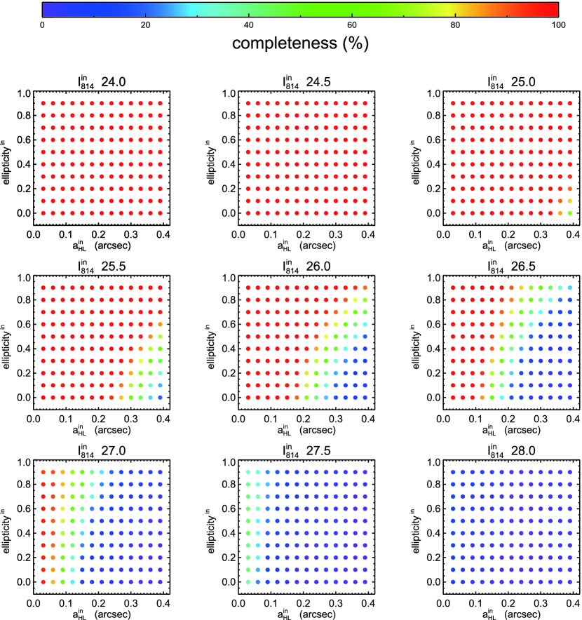
Figure 18.— 2 dimensional map of the detection completeness in the $\epsilon^{\mathrm{in}}$–$a_{\mathrm{HL}}^{\mathrm{in}}$ plane estimated through a Monte Carlo simulation. The map is separately plotted for different input magnitude of $I_{814}^{\mathrm{in}}$.

The resultant detection completenesses as a function of the input parameters of $I_{814}^{\mathrm{in}}$, $a_{\mathrm{HL}}^{\mathrm{in}}$, and $\epsilon^{\mathrm{in}}$ are presented in Figure 18. As expected, the sources with relatively bright input magnitudes of $I_{814}^{\mathrm{in}}\lesssim 25.0$ mag have high detection completenesses of $\approx 100$% regardless of the other input parameters of $a_{\mathrm{HL}}^{\mathrm{in}}$ and $\epsilon^{\mathrm{in}}$. For the fainter sources with $I_{814}\gtrsim 25.0$ mag, the detection completenesses are found to become lower for more extended sources with smaller ellipticities. This is simply because, at a given $I_{814}^{\mathrm{in}}$, the surface brightnesses are lower for the sources with large $a_{\mathrm{HL}}^{\mathrm{in}}$ at a fixed $\epsilon^{\mathrm{in}}$ and for those with small $\epsilon^{\mathrm{in}}$ at a fixed $a_{\mathrm{HL}}^{\mathrm{in}}$. For the sources fainter than the $3\sigma$ limiting magnitude of the ACS images in a $1^{\prime\prime}$ diameter aperture of 27.4 mag, almost all sources are found to be undetected regardless of $a_{\mathrm{HL}}^{\mathrm{in}}$ and $\epsilon^{\mathrm{in}}$.

A.2. Double Component

Similar to the Monte Carlo simulations for single-component sources described in Section A.1, we performed the following simulations in order to estimate the deformation effects in shape via the blending with unresolved double or multiple sources (Section 4.4.2). For simplicity, all artificial sources are assumed to consist of two identical components having the same $a_{\mathrm{HL}}^{\mathrm{in}}$ and $I_{814}^{\mathrm{in}}$ with angular separation of $r_{\mathrm{sep}}$. Each component is assumed to have a perfectly round shape (i.e., $\epsilon^{\mathrm{in}}=0$). As done in Section A.1, the exponential light profile is adopted for each component. We adopt a single value of 0$\farcs$07 for the intrinsic size of each component of $a_{\mathrm{HL}}^{\mathrm{in}}$, which is found to result in a similar distribution in the $\epsilon$–$a_{\mathrm{HL}}$ plane to the observed one. The full ranges (steps) of the other parameters are provided as $I_{814}^{\mathrm{in}}=25.5$–28.0 mag ($\Delta I_{814}^{\mathrm{in}}=0.5$ mag) and $r_{\mathrm{sep}}=0\farcs 03$–0$\farcs$30 ($\Delta r_{\mathrm{sep}}=0\farcs 03$). We prepare 5000 sources for each set of parameters; in total, 300,000 artificial sources are generated. Then, as done in Section A.1, we put these sources on the observed ACS image randomly, convolving the PSF image and adding photon noises and the Galactic dust extinction. We try to extract their images by using SExtractor with the same parameter set described in Section 2. The resultant magnitude $I_{814}^{\mathrm{out}}$, half-light major radius $a_{\mathrm{HL}}^{\mathrm{out}}$, and ellipticity $\epsilon^{\mathrm{out}}$ are measured only for the sources detected as single component using the SExtractor modified by one of the authors.

References

- Acquaviva et al. (2011) Acquaviva, V., Gawiser, E., & Guaita, L. 2011, ApJ, 737, 47
- Atek et al. (2009) Atek, H., Kunth, D., Schaerer, D., et al. 2009, A&A, 506, L1
- Atek et al. (2014) Atek, H., Kunth, D., Schaerer, D., et al. 2014, A&A, 561, A89
- Bertin & Arnouts (1996) Bertin, E., & Arnouts, S. 1996, A&AS, 117, 393
- Bond et al. (2009) Bond, N. A., Gawiser, E., Gronwall, C., et al. 2009, ApJ, 705, 639
- Bond et al. (2012) Bond, N. A., Gawiser, E., Guaita, L., et al. 2012, ApJ, 753, 95
- Capak et al. (2007) Capak, P., Aussel, H., Ajiki, M., et al. 2007, ApJS, 172, 99
- Chary et al. (2005) Chary, R.-R., Stern, D., & Eisenhardt, P. 2005, ApJ, 635, L5
- Chonis et al. (2013) Chonis, T. S., Blanc, G. A., Hill, G. J., et al. 2013, ApJ, 775, 99
- Cowie & Hu (1998) Cowie, L. L., & Hu, E. M. 1998, AJ, 115, 1319
- Dow-Hygelund et al. (2007) Dow-Hygelund, C. C., Holden, B. P., Bouwens, R. J., et al. 2007, ApJ, 660, 47
- Duval et al. (2014) Duval, F., Schaerer, D., Östlin, G., & Laursen, P. 2014, A&A, 562, A52
- Elmegreen et al. (2009) Elmegreen, D. M., Elmegreen, B. G., Marcus, M. T., et al. 2009, ApJ, 701, 306
- Finkelstein et al. (2011) Finkelstein, S. L., Cohen, S. H., Windhorst, R. A., et al. 2011, ApJ, 735, 5
- Finkelstein et al. (2009a) Finkelstein, S. L., Malhotra, S., Rhoads, J. E., Hathi, N. P., & Pirzkal, N. 2009a, MNRAS, 393, 1174
- Finkelstein et al. (2013) Finkelstein, S. L., Papovich, C., Dickinson, M., et al. 2013, Nature, 502, 524
- Finkelstein et al. (2009b) Finkelstein, S. L., Rhoads, J. E., Malhotra, S., & Grogin, N. 2009b, ApJ, 691, 465
- Finkelstein et al. (2008) Finkelstein, S. L., Rhoads, J. E., Malhotra, S., Grogin, N., & Wang, J. 2008, ApJ, 678, 655
- Förster Schreiber et al. (2011) Förster Schreiber, N. M., Shapley, A. E., Genzel, R., et al. 2011, ApJ, 739, 45
- Gawiser et al. (2006) Gawiser, E., van Dokkum, P. G., Gronwall, C., et al. 2006, ApJ, 642, L13
- Grogin et al. (2011) Grogin, N. A., Kocevski, D. D., Faber, S. M., et al. 2011, ApJS, 197, 35
- Gronke & Dijkstra (2014) Gronke, M., & Dijkstra, M. 2014, MNRAS, 444, 1095
- Gronwall et al. (2011) Gronwall, C., Bond, N. A., Ciardullo, R., et al. 2011, ApJ, 743, 9
- Gronwall et al. (2007) Gronwall, C., Ciardullo, R., Hickey, T., et al. 2007, ApJ, 667, 79
- Guaita et al. (2011) Guaita, L., Acquaviva, V., Padilla, N., et al. 2011, ApJ, 733, 114
- Hagen et al. (2014) Hagen, A., Ciardullo, R., Gronwall, C., et al. 2014, ApJ, 786, 59
- Hayes et al. (2014) Hayes, M., Östlin, G., Duval, F., et al. 2014, ApJ, 782, 6
- Hayes et al. (2011) Hayes, M., Schaerer, D., Östlin, G., et al. 2011, ApJ, 730, 8
- Iye et al. (2004) Iye, M., Karoji, H., Ando, H., et al. 2004, PASJ, 56, 381
- Jiang et al. (2013) Jiang, L., Egami, E., Fan, X., et al. 2013, ApJ, 773, 153
- Kaifu et al. (2000) Kaifu, N., Usuda, T., Hayashi, S. S., et al. 2000, PASJ, 52, 1
- Kashikawa et al. (2011) Kashikawa, N., Shimasaku, K., Matsuda, Y., et al. 2011, ApJ, 734, 119
- Kobayashi et al. (2007) Kobayashi, M. A. R., Totani, T., & Nagashima, M. 2007, ApJ, 670, 919
- Kobayashi et al. (2010) Kobayashi, M. A. R., Totani, T., & Nagashima, M. 2010, ApJ, 708, 1119
- Koekemoer et al. (2007) Koekemoer, A. M., Aussel, H., Calzetti, D., et al. 2007, ApJS, 172, 196
- Koekemoer et al. (2011) Koekemoer, A. M., Faber, S. M., Ferguson, H. C., et al. 2011, ApJS, 197, 36
- Kornei et al. (2010) Kornei, K. A., Shapley, A. E., Erb, D. K., et al. 2010, ApJ, 711, 693
- Laursen et al. (2013) Laursen, P., Duval, F., Östlin, G. 2013, ApJ, 766, 124
- Laursen et al. (2009a) Laursen, P., Razoumov, A. O., & Sommer-Larsen, J. 2009a, ApJ, 696, 853
- Laursen & Sommer-Larsen (2007) Laursen, P., & Sommer-Larsen, J. 2007, ApJ, 657, L69
- Laursen et al. (2009b) Laursen, P., Sommer-Larsen, J., & Andersen, A. C. 2009b, ApJ, 704, 1640
- Law et al. (2012) Law, D. R., Steidel, C. C., Shapley, A. E., et al. 2012, ApJ, 759, 29
- Malhotra et al. (2012) Malhotra, S., Rhoads, J. E., Finkelstein, S. L., et al. 2012, ApJ, 750, L36
- Mawatari et al. (2012) Mawatari, K., Yamada, T., Nakamura, Y., Hayashino, T., & Matsuda, Y. 2012, ApJ, 759, 133
- Miyazaki et al. (2002) Miyazaki, S., Komiyama, Y., Sekiguchi, M., et al. 2002, PASJ, 54, 833
- Momose et al. (2014) Momose, R., Ouchi, M., Nakajima, K., et al. 2014, MNRAS, 442, 110
- Murata et al. (2014) Murata, K. L., Kajisawa, M., Taniguchi, Y., et al. 2014, ApJ, 786, 15
- Murayama et al. (2007) Murayama, T., Taniguchi, Y., Scoville, N. Z., et al. 2007, ApJS, 172, 523
- Nilsson et al. (2007) Nilsson, K. K., Møller, P., Möller, O., et al. 2007, A&A, 471, 71
- Nilsson et al. (2009) Nilsson, K. K., Tapken, C., Møller, P., et al. 2009, A&A, 498, 13
- Ono et al. (2013) Ono, Y., Ouchi, M., Curtis-Lake, E., et al. 2013, ApJ, 777, 155
- Ono et al. (2012) Ono, Y., Ouchi, M., Mobasher, B., et al. 2012, ApJ, 744, 83
- Ono et al. (2010a) Ono, Y., Ouchi, M., Shimasaku, K., et al. 2010a, ApJ, 724, 1524
- Ono et al. (2010b) Ono, Y., Ouchi, M., Shimasaku, K., et al. 2010b, MNRAS, 402, 1580
- Ouchi et al. (2013) Ouchi, M., Ellis, R., Ono, Y., et al. 2013, ApJ, 778, 102
- Ouchi et al. (2009) Ouchi, M., Ono, Y., Egami, E., et al. 2009, ApJ, 696, 1164
- Ouchi et al. (2005) Ouchi, M., Shimasaku, K., Akiyama, M., et al. 2005, ApJ, 620, L1
- Ouchi et al. (2008) Ouchi, M., Shimasaku, K., Akiyama, M., et al. 2008, ApJS, 176, 301
- Ouchi et al. (2010) Ouchi, M., Shimasaku, K., Furusawa, H., et al. 2010, ApJ, 723, 869
- Overzier et al. (2008) Overzier, R. A., Bouwens, R. J., Cross, N. J. G., et al. 2008, ApJ, 673, 143
- Patton et al. (2013) Patton, D. R., Torrey, P., Ellison, S. L., Mendel, J. T., & Scudder, J. M. 2013, MNRAS, 433, L59
- Peng et al. (2002) Peng, C. Y., Ho, L. C., Impey, C. D., & Rix, H.-W. 2002, AJ, 124, 266
- Peng et al. (2010) Peng, C. Y., Ho, L. C., Impey, C. D., & Rix, H.-W. 2010, AJ, 139, 2097
- Pentericci et al. (2010) Pentericci, L., Grazian, A., Scarlata, C., et al. 2010, A&A, 514, A64
- Pirzkal et al. (2007) Pirzkal, N., Malhotra, S., Rhoads, J. E., & Xu, C. 2007, ApJ, 667, 49
- Rhoads et al. (2000) Rhoads, J. E., Malhotra, S., Dey, A., et al. 2000, ApJ, 545, L85
- Rhoads et al. (2005) Rhoads, J. E., Panagia, N., Windhorst, R. A., et al. 2005, ApJ, 621, 582
- Scoville et al. (2007b) Scoville, N., Abraham, R. G., Aussel, H., et al. 2007b, ApJS, 172, 38
- Scoville et al. (2007a) Scoville, N., Aussel, H., Brusa, M., et al. 2007a, ApJS, 172, 1
- Shapley et al. (2003) Shapley, A., Steidel, C. C., Pettini, M., & Adelberger, K. L. 2003, ApJ, 588, 65
- Shibuya et al. (2012) Shibuya, T., Kashikawa, N., Ota, K., et al. 2012, ApJ, 752, 114
- Shibuya et al. (2014) Shibuya, T., Ouchi, M., Nakajima, K., et al. 2014, ApJ, 785, 64
- Shimasaku et al. (2006) Shimasaku, K., Kashikawa, N., Doi, M., et al. 2006, PASJ, 58, 313
- Shioya et al. (2009) Shioya, Y., Taniguchi, Y., Sasaki, S. S., et al. 2009, ApJ, 696, 546
- Stanway et al. (2004) Stanway, E. R., Glazebrook, K., Bunker, A. J., et al. 2004, ApJ, 604, L13
- Tadaki et al. (2014) Tadaki, K.-i., Kodama, T., Tanaka, I., et al. 2014, ApJ, 780, 77
- Taniguchi et al. (2005) Taniguchi, Y., Ajiki, M., Nagao, T., et al. 2005, PASJ, 57, 165
- Taniguchi et al. (2015) Taniguchi, Y., Kajisawa, M., Kobayashi, M. A. R., et al. 2015, ApJ, 809, L7
- Taniguchi et al. (2009) Taniguchi, Y., Murayama, T., Scoville, N. Z., et al. 2009, ApJ, 701, 915
- Taniguchi et al. (2007) Taniguchi, Y., Scoville, N., Murayama, T., et al. 2007, ApJS, 172, 9
- van der Wel et al. (2014) van der Wel, A., Chang, Y.-Y., Bell, E. F., et al. 2014, ApJ, 792, L6
- Vanzella et al. (2009) Vanzella, E., Giavalisco, M., Dickinson, M., et al. 2009, ApJ, 695, 1163
- Vargas et al. (2014) Vargas, C. J., Bish, H., Acquaviva, V., et al. 2014, ApJ, 783, 26
- Venemans et al. (2005) Venemans, B. P., Röttgering, H. J. A., Miley, G. K., et al. 2005, A&A, 431, 793
- Verhamme et al. (2012) Verhamme, A., Dubois, Y., Blaizot, J., et al. 2012, A&A, 546, A111
- Yajima et al. (2012a) Yajima, H., Li, Y., Zhu, Q., & Abel, T. 2012a, MNRAS, 424, 884
- Yajima et al. (2012b) Yajima, H., Li, Y., Zhu, Q., et al. 2012b, ApJ, 754, 118
- Yuma et al. (2010) Yuma, S., Ohta, K., Yabe, K., et al. 2010, ApJ, 720, 1016
- Zheng et al. (2010) Zheng, Z., Cen, R., Trac, H., & Miralda-Escudé, J. 2010, ApJ, 716, 574