To test dual supermassive black hole model for broad line AGN with double-peaked narrow [O iii] lines

Abstract

In this manuscript, we proposed an interesting method to test the dual supermassive black hole model for AGN with double-peaked narrow [O iii] lines (double-peaked narrow emitters), through their broad optical Balmer line properties. Under the dual supermassive black hole model for double-peaked narrow emitters, we could expect statistically smaller virial black hole masses estimated by observed broad Balmer line properties than true black hole masses (total masses of central two black holes). Then, we compare the virial black hole masses between a sample of 37 double-peaked narrow emitters with broad Balmer lines and samples of SDSS selected normal broad line AGN with single-peaked [O iii] lines. However, we can find clearly statistically larger calculated virial black hole masses for the 37 broad line AGN with double-peaked [O iii] lines than for samples of normal broad line AGN. Therefore, we give our conclusion that the dual supermassive black hole model is probably not statistically preferred to the double-peaked narrow emitters, and more efforts should be necessary to carefully find candidates for dual supermassive black holes by observed double-peaked narrow emission lines.

1 Introduction

System of dual supermassive black holes is an inevitable stage of co-evolution of supermassive black hole and host galaxy (Silk & Rees, 1998; Hopkins et al., 2006, 2007; Kormendy & Ho, 2013; Lapi et al., 2014). With separations about kilo-pcs of central dual supermassive black holes, models based on central dual supermassive black holes can be efficiently applied to well explain observed double-peaked narrow emission lines. Therefore, the observed double-peaked narrow emission line can be commonly used as an indicator for central dual black holes, such as the reported dual supermassive black hole candidates based on observed double-peaked narrow emission lines combining with properties of high quality images (Zhou et al., 2004; Gerke et al., 2007; Comerford et al., 2009; Xu & Komossa, 2009; Rosario et al., 2010; Comerford et al., 2011; Fu et al., 2011; Barrows et al., 2012; Blecha et al., 2013; Comerford et al., 2013; Liu et al., 2013; Woo et al., 2014). However, there are many other studies (Liu et al., 2010; Fisher et al., 2011; Shen et al., 2011a; Comerford et al., 2012; Fu et al., 2012) which have shown that scenarios with a single AGN can also well explain observed double-peaked narrow emission lines which could be due to radial flows or due to disk structures of central narrow emission line regions.

So far, it is controversial on the origin of double-peaked narrow emission lines, due to system of central dual supermassive black holes (hereafter, DBH model) or due to gas dynamic structures of narrow emission line regions in a single AGN (hereafter, GD model). However, one distinct point can be found between the two proposed models. The DBH model has apparent and strong effects on central broad emission lines from two independent broad emission line regions rotating around central dual black holes, besides apparent effects on narrow emission lines. However, the GD model has NO effects on central broad emission lines. Therefore, to check properties of broad emission lines of double-peaked narrow emitters will provide further information on the origin of double-peaked narrow emission lines.

There are so far more than 3000 low-redshift double-peaked narrow emitters reported in the literature. The main four large samples and corresponding detailed discussions on properties of double-peaked narrow emission lines can be found in Wang et al. (2009) (87 double-peaked narrow emitters), in Smith et al. (2010) (148 double-peaked narrow emitters), in Ge et al. (2012) (about 3030 double-peaked narrow emitters) and in Barrows et al. (2013) (131 double-peaked narrow emitters). However, there are so far no studies on broad emission lines of double-peaked narrow emitters in the literature. Here, we first report interesting studies on properties of broad Balmer lines of a sample of 37 double-peaked narrow emitters selected from SDSS (Sloan Digital Sky Survey) QSOs, in order to test the DBH model for double-peaked narrow emission lines. This paper is organized as follows. Section 2 shows our main hypotheses based on the DBH model, and Section 3 gives our main results for the 37 double-peaked narrow emitters with broad Balmer emission lines selected from SDSS and further discussions on their properties of virial black hole masses, and then Section 4 gives our main conclusions. And in this manuscript, cosmological parameters $H_{0}=70{\rm km\cdot s}^{-1}{\rm Mpc}^{-1}$, $\Omega_{\Lambda}=0.7$ and $\Omega_{m}=0.3$ have been adopted.

2 Hypotheses

Based on the DBH model for double-peaked narrow emission lines, each observed broad emission line of a double-peaked narrow emitter actually includes two components from central two independent BLRs (broad emission line regions) with separation about kilo-pcs. The separation of central dual black holes is large enough, so that for each black hole plus one BLR system, its central virial black hole mass can be well determined by broad line width and continuum luminosity under the widely applied virialization assumption (McLure & Dunlop, 2004; Peterson et al., 2004; Greene & Ho, 2005; Vestergaard & Peterson, 2006; Kelly & Bechtold, 2007; Vestergaard & Osmer, 2009; Rafiee & Hall, 2011; Shen et al., 2011; Ho & Kim, 2015; Wu et al., 2015),

$$\begin{split}M_{{\rm 1}}&=k_{{\rm BH}}\times(V_{{\rm 1}})^{2}\times(\lambda L_{{\rm 1}})^{\sim 0.5}\\ M_{{\rm 2}}&=k_{{\rm BH}}\times(V_{{\rm 2}})^{2}\times(\lambda L_{{\rm 2}})^{\sim 0.5}\\ \end{split}$$ (1)

, where $k_{{\rm BH}}$ is a scale factor, $V$ means broad line width (second moment $\sigma$ or full width at half maximum FWHM), $\lambda L$ represents continuum luminosity at 5100Å which can be used to estimate distance of BLR to central black hole (the well-known R-L relation, Kaspi et al. (2000); Wang & Zhang (2003); Kaspi et al. (2005); Denney et al. (2010); Bentz et al. (2013)). Therefore, central total black hole mass of a double-peaked narrow emitter is $M_{{\rm tot}}=M_{{\rm 1}}+M_{{\rm 2}}$. In addition, in observed spectra of double-peaked narrow emitters, broad emission lines can not be clearly divided into two broad components, because their peak shifted velocities are less than several hundreds kilometers per second, more smaller than broad line widths. Here, due to more larger separations of central dual black holes in double-peaked narrow emitters, we accept that there are the same peak shifted velocities of the two broad components as those of the double-peaked narrow emission lines. Therefore, similar as Equation (1), central black hole mass of a double-peaked narrow emitter can also be estimated through line parameters of observed broad emission lines,

$$M_{{\rm BH}}=k_{{\rm BH}}\times(V_{{\rm obs}})^{2}\times(\lambda L_{{\rm obs}})^{0.5}$$ (2)

. Then, properties of $M_{{\rm tot}}$ and $M_{{\rm BH}}$ should provide further information on the origin of double-peaked narrow emission lines.

It is clear that for a double-peaked narrow emitter, the first direct point under the DBH model we can have is

$$\lambda L_{{\rm obs}}\sim\lambda L_{{\rm 1}}+\lambda L_{{\rm 2}}$$ (3)

, where $\lambda L_{{\rm obs}}$ means the observed continuum luminosity at 5100Å. And then, because broad line width is more larger than peak separation of the two expected broad components under the DBH model, the second point we can have is

$$V_{{\rm obs}}^{2}\sim f_{{\rm 1}}\times V_{{\rm 1}}^{2}+f_{{\rm 2}}\times V_{{\rm 2}}^{2}$$ (4)

where $V_{{\rm obs}}$ means broad line width measured from observed broad emission lines, and $f_{{\rm 1}}$ and $f_{{\rm 2}}=1-f_{{\rm 1}}$ mean flux ratios of the two expected broad components to total broad emission line ($f_{{\rm 1}}$ and $f_{{\rm 2}}$ are values less than 1). Here, we should note whether second moment or FWHM is used as broad line width ($V$, $V_{{\rm obs}}$), the equation above can be well accepted, unless there are much large peak separations. And the equation above can be directly obtained from definition of second moment (Peterson et al., 2004), similar as what we have done in Zhang (2011).

Based on the two points above, we can find that virial black hole mass from observed broad line parameters can be described as

$$\begin{split}M_{{\rm BH}}^{2}&=f_{{\rm 1}}^{2}\times V_{{\rm 1}}^{4}\times\lambda L_{{\rm 1}}+f_{{\rm 2}}^{2}\times V_{{\rm 2}}^{4}\times\lambda L_{{\rm 2}}\\ &=f_{{\rm 1}}^{2}\times M_{{\rm 1}}^{2}+f_{{\rm 2}}^{2}\times M_{{\rm 2}}^{2}\end{split}$$ (5)

. Therefore, a direct and interesting result is that the estimated virial black hole mass $M_{{\rm BH}}$ from observed broad emission lines is more smaller than the true total black hole mass $M_{{\rm tot}}$ in a double-peaked narrow emitter. For example, if $f_{{\rm 1}}=f_{{\rm 2}}=0.5$ (central two broad components have similar continuum emissions at 5100Å) and $M_{{\rm 1}}\sim M_{{\rm 2}}$, we could have $M_{{\rm BH}}\sim M_{{\rm tot}}/2.8$.

Before the end of the Section, we give more clearer results on mass ratio ($M_{{\rm ot}}$) of $M_{{\rm tot}}$ to $M_{{\rm BH}}$. Based on ratios of two peak shifted velocities of double-peaked narrow emission lines of the reported double-peaked narrow emitters (Wang et al., 2009; Smith et al., 2010; Ge et al., 2012), we simply accepted that $M_{{\rm 1}}/M_{{\rm 2}}$ is from 0.2 to 4 under the DBH model. And, we accept that $f_{{\rm 1}}$ is from 0.2 to 0.8. Then, ten thousand values are randomly created for $M_{{\rm 1}}/M_{{\rm 2}}$, and for $f_{{\rm 1}}$. Distribution of the ten thousand calculated ratios of $M_{{\rm tot}}$ to $M_{{\rm BH}}$ is shown in Fig. 1. It is clear that the mean value of $M_{{\rm ot}}$ is around 2.7 (minimum value larger than 1.5), and virial black hole masses from observed broad emission lines ($M_{{\rm BH}}$) should be statistically smaller than true virial black hole masses ($M_{{\rm tot}}$). Therefore, under the virialization assumption for central broad line regions and the DBH model for double-peaked narrow emission lines, it is interesting to check whether virial black hole masses of double-peaked narrow emitters are statistically smaller than normal broad line AGN with single-peaked narrow lines.

3 Main Results

3.1 Our Data Sample

Based on the samples of double-peaked narrow emitters reported in the literature, especially from the sample of Smith et al. (2010), we can collect double-peaked narrow emitters with broad Balmer lines. Actually, in the large sample of Ge et al. (2012), there are many emitters reported as type 1 AGN. However, when we checked their SDSS spectra, only weak broad components (second moment less than 800${\rm km/s}$) around H$\alpha$ can be found, no broad components around H$\beta$ can be found. It is hard to confirm the weak broad components from central BLRs of those objects. Thus, we mainly select targets from the double-peaked narrow emitters classified as QSOs in SDSS database (York et al., 2000; Gunn et al., 2006; Eisenstein et al., 2011; Smee et al., 2013; Alam et al., 2015). Then, from low-redshift QSOs ($z<0.35$) in SDSS DR7 (Data Release 7, Schneider et al. (2010)), there are 37 QSOs reported as double-peaked narrow emitters in Smith et al. (2010) included in our main sample. Here, the restriction of $z<0.35$ enables us to check both the broad H$\beta$ and the broad H$\alpha$, which will ensure the accuracy of following measured line widths of broad lines (sometimes effects of much extended wings of [O iii] lines can not be clearly removed, if only broad H$\beta$ is checked). Basic information of 37 targets is listed in Table 1.

Then, as discussed in Section 2, it is necessary to determine line width of broad Balmer lines and continuum luminosity at 5100Å, in order to estimate virial black hole masses. Here, one point we should note is that Shen et al. (2011) have reported virial black hole masses of QSOs in SDSS DR7 by continuum luminosity and FWHM of broad emission lines. In order to do convenient comparisons of virial black hole masses between the 37 double-peaked narrow emitters and normal broad line QSOs in Shen et al. (2011), FWHM is used as the line width of broad Balmer lines in this manuscript.

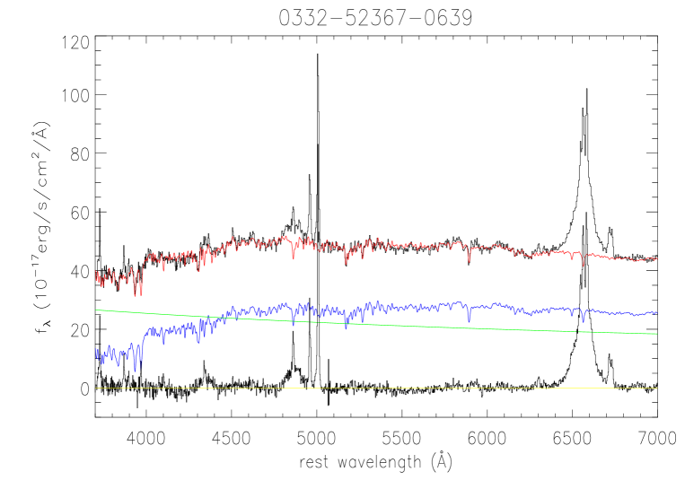
Figure 2: An example shows the subtraction of stellar lights in SDSS 0332-52367-0639 (plate-mjd-fiberid) by the SSP method. From top to bottom, solid lines in black and in red show the observed spectrum and the best fitted results respectively, solid lines in blue and in green show the determined stellar lights and the power law component respectively, solid lines in black and in yellow show the pure line spectrum and $f_{\lambda}=0$.

Before measuring line parameters, we can find that there are 9 of the 37 double-peaked narrow emitters, of which spectra include apparent contributions of star lights. Therefore, one procedure is first applied to subtract stellar lights in their spectra. Here, the SSP method (Simple Stellar Population) is applied with 39 simple stellar template spectra from Bruzual & Charlot (2003) with stellar population ages from 5Myr to 12Gyr and with three metallicities (Z=0.008, 0.05, 0.02). More detailed and recent descriptions on the SSP method can be found in Bruzual & Charlot (2003); Cid Fernandes et al. (2005); Richards et al. (2009); Cappellari et al. (2012); Zhang (2014) etc.. Fig. 2 shows an example on the subtraction of stellar lights by the SSP method. Then, line parameters can be determined from line spectra after subtractions of stellar lights.

Emission lines around H$\alpha$ and H$\beta$ are then mainly focused on, and fitted simultaneously by the following model functions. Three (or more if necessary, after checking fitted results by three Gaussian functions) broad Gaussian functions are applied to describe each broad Balmer line, two Gaussian functions are applied to each double-peaked narrow emission line, and two additional Gaussian components are applied to probable extended wings of the [O iii] doublet, one broad Gaussian function is applied to describe the weak He ii line, one power law function is applied to describe the AGN continuum emission, and then the Fe ii template discussed in Kovacevic et al. (2010) is applied to describe the probable optical Fe ii lines. And moreover, if one narrow emission line is single-peaked, only one Gaussian function is applied to the narrow emission line. When the functions above are applied to fit the emission lines around H$\beta$ and H$\alpha$ simultaneously, the following restrictions are applied (parameters tied to one another in the MPFIT procedure), (1): blue (red) components of the double-peaked narrow emission lines have the same redshift, (2): corresponding broad components of broad H$\alpha$ and broad H$\beta$ have the same redshifts, when they are fitted by multiple broad Gaussian functions, (3): the flux ratios of components of the [O iii] (the [N ii] ) doublet are fixed to the theoretical values $f_{{\rm 5007}}/f_{{\rm 4959}}=3$ ($f_{{\rm 6585}}/f_{{\rm 6549}}=3$), (4): there are the same line widths of the blue (red) components of the double-peaked narrow Balmer lines (the [O iii] or [O i] or [S ii] doublets). Here, we should note that line flux of broad components are not tied between broad Balmer lines. In other words, different flux ratios are allowed for components of broad Balmer lines. And, in our procedure, not the severe restriction of ’the same line profile’ but ’similar line profile’ is applied to broad Balmer lines.

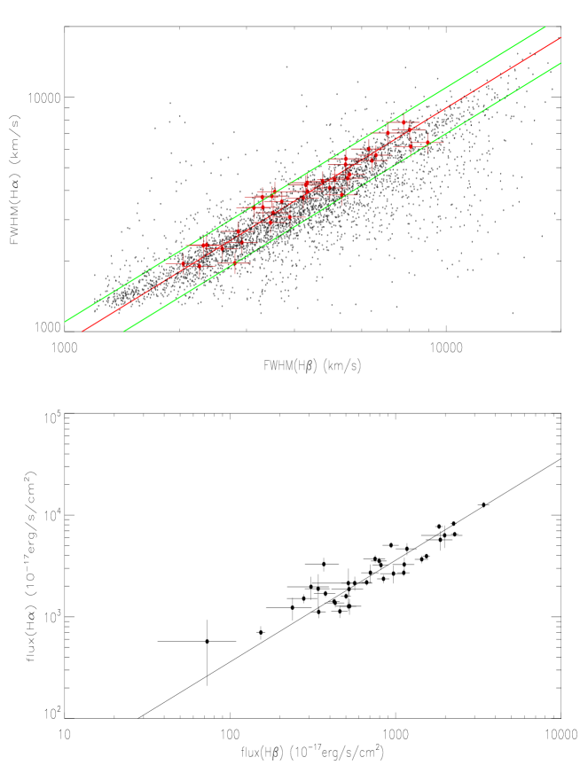
Figure 4: On broad line width correlation and broad line flux correlation between broad H$\beta$ and broad H$\alpha$. In top panel, red circles are for the 37 double-peaked narrow emitters, dots are for the 3477 normal broad line AGN from SDSS DR7, and solid line in red shows $FWHM({\rm H\alpha})=0.91\times FWHM({\rm H\beta})$. And the two green lines represent $FWHM({\rm H\beta})=0.8\times FWHM({\rm H\alpha})$ and $FWHM({\rm H\beta})=1\times FWHM({\rm H\alpha})$ respectively. In bottom panel, solid line shows $flux({\rm H\alpha})=3.3\times flux({\rm H\beta})$.

Obviously, there are three main different points between our emission line fitting procedure and the procedure in Shen et al. (2011). First and foremost, more than three Gaussian functions are allowed to fit broad Balmer lines, which can lead to more better fitted results for broad Balmer lines with more extended components. Besides, more recent and high-quality Fe ii template in Kovacevic et al. (2010) is applied to describe optical band Fe ii components, rather than the template in Boroson & Green (1992). Last but not the least, the broad H$\alpha$ and H$\beta$ are fitted simultaneously, which can reduce effects of extended [O iii] components on broad H$\beta$ as much as possible and lead to similar line profiles of broad Balmer lines (for example, by the procedure of Shen et al. (2011), some QSOs have much different broad Balmer line widths as the results shown in following Fig. 4).

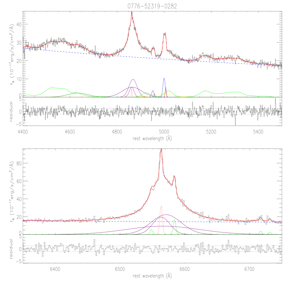
Figure 3: Examples of the best fitted results for emission lines around H$\beta$ (top panel) and around H$\alpha$ (bottom panel) in SDSS 0776-52319-0282. In each panel, top region shows the spectrum and the best fitted results, and bottom region shows the corresponding residuals. For the line spectrum and the best fitted results, solid line in black, thick solid line in red, solid lines in purple, in pink and dashed line in blue show the observed spectrum, the best fitted results, the determined broad Balmer components, the narrow Balmer component, and the AGN continuum emission respectively. And, for the best results for emission lines around H$\beta$, solid line in green, thin solid line in blue and in red, and thick solid line in dark green and in yellow show the Fe ii lines, the blue components and the red components of the [O iii] doublet, the broad He ii line, and the extended components of the [O iii] doublet respectively. And for the best fitted results for emission lines around H$\alpha$, solid line in green shows the [N ii] ,[S ii] doublets. And for residuals, horizontal dotted lines show $residual=\pm 1$.

Then, through the Levenberg-Marquardt least-squares minimization technique (the MPFIT package, Markwardt (2009)), the double-peaked and/or single-peaked narrow emission lines and the broad Balmer lines can be well determined. Here, we do not show the fitted results for emission lines of all the 37 double-peaked narrow emitters, but Fig. 3 shows an example on the best fitted results for emission lines around H$\beta$ and around H$\alpha$ in SDSS 0776-52319-0282 (plate-mjd-fiberid), of which there are double-peaked [O iii] lines, but single-peaked other narrow emission lines, and apparent Fe ii lines. Then, for the 37 double-peaked narrow emitters, continuum luminosities at 5100Å can be calculated by the determined power law AGN continuum emissions. And FWHMs of broad Balmer lines can be well determined by broad line profiles, after subtractions of the narrow emission lines, the power law continuum emissions, the Fe ii lines and the He ii lines.

Then, we can check whether the determined broad line parameters are reliable. Here, we do not consider uncertainties of FWHM and continuum luminosity, because the uncertainties have few effects on statistic properties of virial black hole masses. The determined FWHMs, along with the determined line fluxes of broad Balmer lines and the continuum emission at 5100Å, are listed in Table 1. We first check line width correlation and line flux correlation between broad H$\beta$ and broad H$\alpha$, in order to ensure the accuracy of broad line parameters. Fig. 4 shows the correlations. It is clear that there are strong linear correlations between the broad Balmer lines. The Spearman rank correlation coefficients are about 0.96 with $P_{{\rm null}}\sim 10^{-21}$ and 0.88 with $P_{{\rm null}}\sim 10^{-12}$ for the broad line width correlation and for the broad line flux correlation respectively. And moreover, the two correlations can be well described by $FWHM({\rm H\alpha})\sim 0.9\times FWHM({\rm H\beta})$ and $flux({\rm H\alpha})\sim 3.3\times flux({\rm H\beta})$, which are consistent with the results shown in Greene & Ho (2005) for QSOs. Therefore, the measured broad line widths and broad line fluxes are reliable. And moreover, in top panel of Fig. 4, we also show broad line widths of 3477 normal broad line AGN from Shen et al. (2011). We can find that there are more larger scatters for the broad line width correlation for the normal broad line AGN, without restriction of similar line profiles of broad Balmer lines. So that, the restriction of similar line profiles of broad Balmer lines can well ensure the accuracy of the measured broad line parameters.

3.2 Virial black hole masses

Based on the continuum luminosity at 5100Å ($\lambda L_{{\rm 5100}}$) and the measured line with of broad H$\beta$, virial black hole masses of the 37 double-peaked narrow emitters can be estimated by the equation in Vestergaard & Peterson (2006) (VP06) and in Shen et al. (2011),

$$\begin{split}M_{{\rm BH}}&=A+B\log(\frac{\lambda L_{{\rm 5100}}}{10^{44}\ {\rm erg/s}})+2\log(\frac{FWHM({\rm H\beta})}{\rm km/s})\\ &A=0.91,\ \ B=0.5\end{split}$$ (6)

. The main reason to use the equation in VP06 is mainly due to its application of $R_{{\rm BLR}}\propto(\lambda L_{{\rm 5100}})^{0.5}$ identical to more recent R-L relation in Bentz et al. (2013). The estimated virial black hole masses are also listed in the Table 1 for the 37 double-peaked narrow emitters. The mean value of virial black hole masses of the 37 double-peaked narrow emitters is about $\log(M_{{\rm BH}}/{\rm M_{{\rm\odot}}})\sim 8.11$.

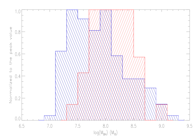
Figure 5: Comparison of virial black hole masses between the 37 double-peaked narrow emitters (in red color) and the 298 normal broad line AGN from SDSS DR7 (in blue color).

Then, we can check whether are there different properties of virial black hole masses of normal broad line AGN with single-peaked narrow emission lines. A parent sample of normal broad line AGN can be created from the dataset of Shen et al. (2011) by the the following three criteria, (1): objects are not double-peaked narrow emitters (information from key parameter of special_interest_flag), (2): objects have redshifts less than 0.35, (3): objects have similar measured broad Balmer line widths ($0.8<\frac{FWHM({\rm H\alpha})}{FWHM({\rm H\beta})}=F_{ab}<1$, where range of [0.8, 1] is the range covered all the 37 double-peaked narrow emitters in the top panel of Fig. 4), which will ensure the accuracy of broad Balmer line widths. Through the criteria (1) and (2), 3477 normal broad line AGN are selected, of which broad line widths of broad Balmer lines are shown in the top panel of Fig. 4. And then, through the criterion (3), there are 298 normal broad line AGN included in our parent sample. The mean value is about $\log(M_{{\rm BH}}/{\rm M_{{\rm\odot}}})\sim 7.88$ of the virial black hole masses estimated by the Equation (6) for the 298 normal broad line AGN in Shen et al. (2011). And Fig. 5 shows distributions of virial black hole masses of the 37 double-peaked narrow emitters and the 298 normal broad line AGN. We can find clearly statistically larger virial black hole masses in the 37 double-peaked narrow emitters with broad Balmer lines than in the normal broad line AGN.

Then, the Student’s T-statistic technique is applied to check whether the 37 double-peaked narrow emitters and the normal broad line AGN have significantly different mean virial black hole masses. For the parent sample including 298 normal broad line AGN and the sample of the 37 double-peaked narrow emitters, the calculated T-statistic value and its significance are 3.59 and $7.1\times 10^{-4}$ respectively, which indicate that the 37 double-peaked narrow emitters and the normal broad line AGN have much different mean values of their black hole masses with confidence level higher than 99.9%.

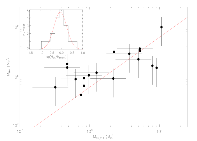
Figure 6: Comparison of our determined virial black hole masses $M_{{\rm BH}}$ and the black hole masses $M_{{\rm BH,S11}}$ reported in Shen et al. (2011) for the 18 double-peaked narrow emitters included in Shen et al. (2011). The red solid line shows $M_{{\rm BH,S11}}=M_{{\rm BH}}$. Here, we assume the uncertainty of our determined virial black hole mass about 53% (mean value from Shen et al. 2011). Top-left corner shows distribution of $\log(M_{{\rm BH}}/M_{{\rm BH,S11}})$ which can be well described by a Gaussian function with second moment 0.3 (solid line in red in the corner).

Before proceeding further, we can find that among the 37 double-peaked narrow emitters listed in Table 1, there are 18 objects of which virial black hole masses can also be found in Shen et al. (2011). Here, the 37 objects in our main sample are selected from 21592 QSOs with redshift less than 0.7 in SDSS DR7 (see descriptions in Smith et al. (2010)), however, the catalogue of Shen et al. (2011) includes only 15798 QSOs with redshift less than 0.7. Therefore, not all the 37 objects are included in the QSO catalogue of Shen et al. (2011). Although, the same equation in VP06 is applied to estimate the virial black hole masses of the 37 double-peaked narrow emitters and the normal broad line AGN in Shen et al. (2011), a bit different procedures are applied to determine the line width of broad H$\beta$. Thus, it is necessary to check effects of different emission line fitting procedures on final virial black hole masses. Fig. 6 shows the comparison of our determined virial black hole masses $M_{{\rm BH}}$ and the reported masses $M_{{\rm BH,S11}}$ in Shen et al. (2011) for the 18 double-peaked narrow emitters. Here, values of $M_{{\rm BH,S11}}$ of the 18 objects are also listed in Table 1. The Spearman rank correlation coefficient for the correlation is about 0.67 with $P_{{\rm null}}\sim 2\times 10^{-3}$. And moreover, the top-left corner of Fig. 6 shows distribution of $\log(M_{{\rm BH}}/M_{{\rm BH,S11}})$ which can be well described by a Gaussian function with second moment 0.3. Therefore, $M_{{\rm BH}}\sim M_{{\rm BH,S11}}$ can be accepted for the 18 objects. Moreover, if we check the mass ratio of $M_{{\rm BH,S11}}$ to $M_{{\rm BH}}$, we will find the mean value of the ratio is about 1.62. Thus, we can safely accept that there are different mean virial black hole masses between the 37 double-peaked narrow emitters and the 298 normal broad line AGN, even with considerations of effects of different emission line fitting procedures.

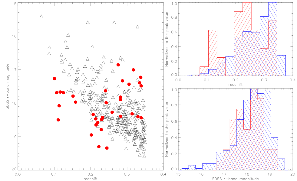
Figure 7: Properties of redshift and SDSS r-band magnitude of the 37 double-peaked narrow emitters and the 298 normal broad line AGN. Left panel shows the correlation between redshift and SDSS r-band magnitude for the 37 double-peaked narrow emitters (red circles) and the 298 normal broad emission line AGN (triangles). Top right panel shows the redshift distributions of the 37 double-peaked narrow emitters (red color) and the 298 normal broad line AGN (blue color). And bottom right panel shows the magnitude distribution of the 37 double-peaked narrow emitters (red color) and the 298 normal broad line AGN (blue color).

Moreover, we should note that there are different distributions of redshift and magnitude between the 37 double-peaked narrow emitters and the 298 normal broad line AGN. The distributions are shown in Fig. 7. By two-sided Kolmogorov-Smirnov statistic technique, we can find that probability is less than 1% that the 37 double-peaked narrow emitters and the 298 normal road line AGN have the same redshift distribution, and probability is less than 20% that the 37 double-peaked narrow emitters and the 298 normal road line AGN have the same SDSS r-band magnitude distribution.

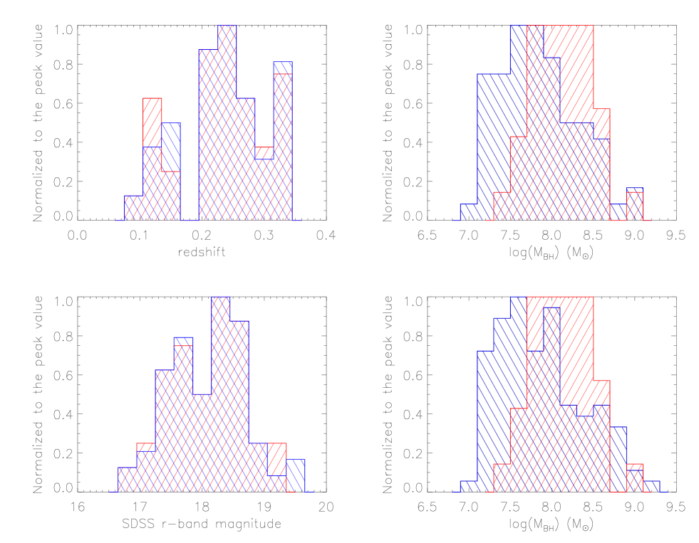
Figure 8: Results on the first subsample and the second subsample. Top left and top right panels show the same redshift distributions and the comparison of black hole mass distributions of the 37 double-peaked narrow emitters and the first subsample of 74 normal broad line AGN respectively. Bottom left and bottom right panels show the same SDSS r-band magnitude distributions and the comparison of black hole mass distributions of the 37 double-peaked narrow emitters and the second subsample of 111 normal broad emission line AGN. In each panel, red and blue colors represent the results for the 37 double-peaked narrow emitters and for the objects in the subsamples respectively.

In order to consider effects of different distributions of redshift and/or magnitude on virial black hole mass comparisons as much as possible, three subsamples are created from the 298 normal broad line AGN as follows. To consider effects of different redshift distribution, the first subsample is created to include 74 normal broad line AGN, and the subsample has the same redshift distribution as that of the 37 double-peaked narrow emitters with probability larger than 92%. The mean virial black hole mass of the subsample is about $\log(M_{{\rm BH}}/{\rm M_{\odot}})\sim 7.84$. And the calculated T-statistic value and its significance are 3.39 and $1\times 10^{-3}$ respectively for distributions of virial black hole masses of the 37 double-peaked narrow emitters and the normal broad line AGN in the subsample, which indicates that the 37 double-peaked narrow emitters and the normal broad line AGN in the subsample have much different mean virial black hole masses with confidence level higher than 99.8%. In addition, in order to consider effects of different magnitude distribution, the second subsample is created to include 111 normal broad line AGN, and the subsample has the same SDSS r-band magnitude distribution as that of the 37 double-peaked narrow emitters with probability larger than 99%. The mean virial black hole mass of the subsample is about $\log(M_{{\rm BH}}/{\rm M_{\odot}})\sim 7.87$. And the the calculated T-statistic value and its significance are 3.23 and $2\times 10^{-3}$ respectively for distributions of virial black hole masses of the 37 double-peaked narrow emitters and the normal broad line AGN in the subsample, which indicates that the 37 double-peaked narrow emitters and the normal broad line AGN in the subsample have much different mean virial black hole masses with confidence level higher than 99.7%. The results on the first subsample and the second subsample are shown in Fig. 8. Furthermore, in order to consider effects of both different redshift distribution and different magnitude distribution, the third subsample is created to include 37 normal broad line AGN, and the subsample has both the same SDSS r-band magnitude distribution and the same redshift distribution as those of the 37 double-peaked narrow emitters with probability larger than 70%. The mean virial black hole mass of the subsample is about $\log(M_{{\rm BH}}/{\rm M_{\odot}})\sim 7.88$. And the the calculated T-statistic value and its significance are 2.28 and $3\times 10^{-2}$ respectively for distributions of virial black hole masses of the 37 double-peaked narrow emitters and the normal broad line AGN in the subsample, which indicates that the 37 double-peaked narrow emitters and the normal broad line AGN in the subsample also have much different mean virial black hole masses with confidence level higher than 97%. The results on the third subsample are shown in Fig. 9. Thus, with considerations of different redshift and/or magnitude distributions, the double-peaked narrow emitters have statistically larger virial black hole masses than the normal broad line AGN.

3.3 Further discussions

In the subsection, there are three points we should note. First and foremost, the Equation (6) discussed in Vestergaard & Peterson (2006) is applied in the paper, due to its application of the R-L relation identical to the more recent results in Bentz et al. (2013). In order to confirm that there are few effects of different equations applied to estimate virial black hole masses on our final results. Further discussions are given as follows. Mean virial black hole mass of a sample of broad line AGN can be estimated by Equation (6) with different values of A and B

$$\overline{M_{{\rm BH}}}=A+B\times\log(\overline{\frac{\lambda L_{{\rm 5100}}}{{10^{44}\ {\rm erg/s}}}})+2\times\log(\overline{FWHM})$$ (7)

. Then, mean virial black hole mass of the 37 double-peaked narrow emitters is about $\overline{M_{{\rm BH,dbp}}}\sim A+0.155\times B+7.323$, and mean virial black hole mass is about $\overline{M_{{\rm BH,AGN}}}\sim A+0.266\times B+6.969$ for the normal broad emission line AGN in the third subsample discussed above with considerations of effects of different distributions of redshift and magnitude. In order to find smaller $\overline{M_{{\rm BH,dbp}}}$ than $\overline{M_{{\rm BH,AGN}}}$, we should have $B>3.2$. Similar results can be found with considering objects in the first subsample and the second subsample. However, more recent observational results in Bentz et al. (2013) have shown that $B\sim 0.533$. In other words, if we accepted the R-L relation $R_{{\rm BLR}}\propto\lambda L^{B}$ with $B\sim 0.5$, it is hard to find smaller statistical virial black hole masses of the 37 double-peaked narrow emitters.

Besides, our main sample includes only 37 double-peaked narrow emitters, perhaps the larger virial black hole masses of the double-peaked narrow emitters are due to the selected double-peaked narrow emitters with larger broad line widths. The mean FWHM of broad H$\beta$ is about 4580${\rm km/s}$ for the 37 double-peaked narrow emitters, however, the mean FWHM of broad H$\beta$ is 3000${\rm km/s}$ for the 298 normal broad emission line AGN in the parent sample. We try to discuss the different broad line widths as follows. On the one hand, when we select the 37 double-peaked narrow emitters, the objects with double-peaked [O iii] lines classified as SDSS QSOs are firstly considered. Then, from the sample of double-peaked narrow emitters, the objects with broad Balmer lines are selected. Therefore, there are no effects of sample selection on the broad line width. On the other hand, under the DBH model for the double-peaked narrow emission lines, in order to explain the broader broad Balmer lines of the 37 double-peaked narrow emitters than normal broad line AGN (from 3000${\rm km/s}$ to 4580${\rm km/s}$), the peak separation of central two broad components could be larger than 2000${\rm km/s}$, which is more larger than the reported peak separations of the double-peaked narrow emission lines. Therefore, although we have no clear ideas why there are broader broad Balmer lines in the double-peaked narrow emitters, the results on different broad line widths between the double-peaked narrow emitters and the normal broad emission line AGN can not support the DBH model. And more efforts should be done to enlarge the sample of the double-peaked narrow emitters with broad Balmer lines, in order to provide more further information on broad emission line properties.

Last but not least, the main objective of this paper is to check the DBH model for the double-peaked narrow emitters, due to the expected smaller virial black hole masses. However, when we try to accept the smaller virial black hole masses in the double-peaked narrow emitters, there is one another assumption that the normal broad line AGN could not have common dual supermassive black holes with separation distance large enough to ensure two independent central BLRs. In other words, there is one unique BLR in central region of normal broad line AGN, however, there are two independent BLRs in central regions of the double-peaked narrow emitter under the DBH model. Therefore, even the BBH systems (binary black hole systems with separation distance about pcs or sub-pcs) are common in normal broad line AGN, smaller virial black hole masses through the broad Balmer line width and the continuum luminosity could be expected for the double-peaked narrow emitters.

4 Conclusions

Finally, we give our main conclusions as follows. On the one hand, through the kinematic model on the dual supermassive black holes, smaller central virial black hole masses could be expected in the double-peaked narrow emitters than in the normal broad line AGN, through the virialization method applied with the observed broad Balmer line width and the observed continuum luminosity. On the other hand, the virial black hole mass comparisons between the double-peaked narrow emitters and the normal broad line AGN show statistically larger virial black hole masses in the double-peaked narrow emitters, which are against the expected results by the DBH model. Therefore, the model on the dual supermassive black holes is not statistically preferred to the double-peaked narrow emitters.

Table 1: Parameters of the 37 double-peaked narrow emitters

pmf	z	Mag	$\lambda L$	$V_{\beta}$	$f_{\beta}$	$V_{\alpha}$	$f_{\alpha}$	$\log(M_{{\rm BH}})$	$\log(M_{{\rm BH,S11}})$
0332-52367-0639*	0.100	17.27	43.44	5510	750$\pm$111	4512	3712$\pm$331	8.11
0452-51911-0080	0.158	17.97	43.21	7029	308$\pm$86	7034	1971$\pm$502	8.21
0472-51955-0101	0.222	19.30	43.20	8938	278$\pm$57	6401	1512$\pm$151	8.41
0512-51992-0632	0.240	17.63	44.27	5446	2238$\pm$92	5162	8247$\pm$236	8.52	8.72
0553-51999-0048*	0.219	18.58	43.16	3308	376$\pm$55	3389	1691$\pm$131	7.53
0605-52353-0126	0.329	18.40	44.21	2046	501$\pm$35	1948	1594$\pm$111	7.64	7.88
0607-52368-0625	0.275	16.85	44.71	3134	2270$\pm$113	3373	6478$\pm$267	8.26	7.68
0609-52339-0435	0.230	18.49	43.95	3493	519$\pm$57	3786	1268$\pm$129	7.97	7.92
0616-52374-0415	0.214	18.65	43.70	6262	237$\pm$72	6005	1231$\pm$309	8.35
0616-52442-0437	0.214	18.65	43.78	6540	425$\pm$32	5654	1413$\pm$77	8.43
0623-52051-0224	0.116	17.67	43.72	5324	1860$\pm$339	3830	5717$\pm$1228	8.22
0776-52319-0206	0.232	18.42	43.55	3706	340$\pm$57	3584	1889$\pm$728	7.82	7.92
0776-52319-0282	0.338	17.48	44.59	2589	1126$\pm$167	2257	3268$\pm$539	8.03	7.99
0793-52370-0293	0.305	17.43	44.53	4950	1974$\pm$549	4099	6322$\pm$1564	8.56	8.72
0978-52431-0633	0.281	17.82	44.30	2851	703$\pm$83	2675	2713$\pm$553	7.97
0978-52441-0622	0.281	17.89	44.31	2310	843$\pm$70	2329	2364$\pm$224	7.79	7.51
1295-52934-0580	0.242	17.99	44.19	5578	1118$\pm$94	4677	2708$\pm$210	8.50	8.35
1426-52993-0110	0.282	18.39	44.09	4285	794$\pm$85	4223	3542$\pm$285	8.22	8.90
1446-53080-0266	0.317	17.01	44.68	3553	3399$\pm$269	3949	12593$\pm$863	8.35	8.70
1605-53062-0443	0.313	18.32	44.23	2914	565$\pm$95	2400	2142$\pm$334	7.95	7.80
1622-53385-0533*	0.201	18.95	43.10	4219	72$\pm$36	3710	572$\pm$362	7.71
1643-53143-0532	0.259	18.27	44.19	3464	969$\pm$162	2919	2660$\pm$529	8.08	8.10
1716-53827-0140*	0.151	17.79	43.56	8071	522$\pm$112	6156	1870$\pm$275	8.50
1762-53415-0388*	0.113	18.08	43.15	4742	368$\pm$84	4381	3295$\pm$503	7.84
1762-53415-0597	0.287	17.33	44.48	3297	1436$\pm$130	3745	3676$\pm$315	8.18	7.68
1853-53566-0561	0.334	17.39	44.55	8013	1827$\pm$92	7251	7731$\pm$432	8.99	9.03
2001-53493-0154	0.214	18.47	43.94	5456	526$\pm$92	5456	1271$\pm$222	8.35
2004-53737-0634	0.125	17.69	43.79	3892	1534$\pm$75	3077	3945$\pm$148	7.99
2022-53827-0553*	0.206	18.34	42.99	7732	517$\pm$205	7804	2144$\pm$830	8.18	8.96
2341-53738-0523	0.338	18.44	44.27	5103	668$\pm$46	4455	2179$\pm$151	8.46	8.57
2365-53739-0359*	0.110	18.50	43.23	4325	815$\pm$89	4313	3224$\pm$340	7.79
2527-54569-0262	0.229	18.79	43.89	6386	430$\pm$58	5366	1371$\pm$132	8.46
2776-54554-0251*	0.106	17.69	43.29	3520	937$\pm$104	3211	5058$\pm$329	7.64
2793-54271-0614*	0.244	19.34	43.31	2356	342$\pm$34	2342	1116$\pm$146	7.31
2947-54533-0050	0.230	18.49	43.81	2794	460$\pm$51	1960	1132$\pm$156	7.70
2953-54560-0530	0.337	17.23	44.70	2257	1169$\pm$168	1900	4659$\pm$626	7.96	8.34
3211-54852-0404	0.232	18.43	43.34	4325	153$\pm$9	3959	701$\pm$104	7.85

Note: The first column shows the SDSS plate-mjd-fiberid, the second column shows the redshift, the third column shows the SDSS r-band psf magnitude, the fourth column shows the continuum luminosity at 5100Å ($\log(\lambda L_{{\rm 5100}})$) in unit of ${\rm erg/s}$, the fifth and the sixth columns show the line width in unit of ${\rm km/s}$ and the line flux in unit of ${\rm 10^{-17}erg/s/cm^{2}}$ of the broad H$\beta$, the seventh and the eighth columns show the line width and the line flux of the broad H$\alpha$, the ninth column shows the virial black hole mass $\log(M_{{\rm BH}})$ in unit of ${\rm M_{\odot}}$, the final column shows the virial black hole mass $\log(M_{{\rm BH,S11}})$ in unit of ${\rm M_{\odot}}$ reported in Shen et al. (2011).

Symbol of * means the SDSS spectrum of the object includes apparent contributions of stellar lights.

Figure 1: On distribution of the black hole mass ratio $M_{{\rm ot}}$.

Figure 9: Results on the third subsample with the same distributions of magnitude and redshift as those of the 37 double-peaked narrow emitters. Left, middle and right panels show the same redshift and the same magnitude distributions and the comparison of black hole mass distributions. In each panel, red and blue colors represent the results for the 37 double-peaked narrow emitters and for the objects in the third subsample respectively.

References

- Alam et al. (2015) Alam S., Albareti F. D., Allende Prieto C., Andres F., Anderson S. F., et al., 2015, ApJS, 219, 12
- Barrows et al. (2012) Barrows R. S., Stern D., Madsen K., Harrison F., Assef R. J., et al., 2012, ApJ, 744, 7
- Barrows et al. (2013) Barrows R. S., Lacy S. C. H., Kennefick J., Comerford J. M., Kennefick D., Berrier J. C., 2013, ApJ, 769, 95
- Bentz et al. (2013) Bentz M. C., Denney K. D., Grier C. J., Barth A. J., Peterson B. M., et al., 2013, ApJ, 767, 149
- Blecha et al. (2013) Blecha L., Civano F., Elvis M., Loeb A., 2013, MNRAS, 428, 1341
- Boroson & Green (1992) Boroson T. A., & Green R. F., 1992, ApJS, 80, 109
- Bruzual & Charlot (2003) Bruzual G., & Charlot S. 2003, MNRAS, 344, 1000
- Cappellari et al. (2012) Cappellari M., McDermid R. M., Alatalo K., Blitz L., Bois M., et al., 2012, Nature, 484, 485
- Cid Fernandes et al. (2005) Cid Fernandes R., Mateus A., Sodre L., Stasinska G., Gomes J. M., 2005, MNRAS, 358, 363
- Comerford et al. (2011) Comerford J. M., Pooley D., Gerke B. F., Madejski G. M., 2011, ApJL, 737, 19
- Comerford et al. (2009) Comerford J. M., Gerke B. F., Newman J. A., Davis M., et al., 2009, ApJ, 698, 956
- Comerford et al. (2012) Comerford J. M., Gerke B. F., Stern D., Cooper M. C., Weiner B., et al., 2012, ApJ, 753, 42
- Comerford et al. (2013) Comerford J. M., Schluns K., Greene J. E., Cool R. J., 2013, ApJ, 777, 64
- Denney et al. (2010) Denney K. D., Peterson B. M., Pogge R. W., Adair A., Atlee D. W., et al., 2010, ApJ, 721, 715
- Eisenstein et al. (2011) Eisenstein D. J., Weinberg D. H., Agol E., Aihara H., Allende P. C., et al., 2011, AJ, 142, 72
- Fisher et al. (2011) Fischer T. C., Crenshaw D. M., Kraemer S. B. et al. 2011, ApJ, 727, 71
- Fu et al. (2011) Fu H., Myers A. D., Djorgovski S. G., Yan L., 2011, 733, 103
- Fu et al. (2012) Fu H., Yan L., Myers A. D., Stockton A., Djorgovski S. G., Rich J. A., 2012, ApJ, 745, 67
- Ge et al. (2012) Ge J. Q., Hu C., Wang J. M., Bai J. M., Zhang S., 2012, ApJS, 201, 31
- Gerke et al. (2007) Gerke B. F., Newman J. A., Lotz J., Yan R. B., Barmby P., et al., 2007, ApJL, 660, 23
- Greene & Ho (2005) Greene J. E. & Ho L. C., 2005, ApJ, 630, 122
- Gunn et al. (2006) Gunn J. E., Siegmund W. A., Mannery E. J., Owen R. E., Hull C. L., et al., 2006, AJ, 131, 2332
- Ho & Kim (2015) Ho L. C. & Kim M., 2015, ApJ, 805, 123
- Hopkins et al. (2006) Hopkins P. F., Hernquist L., Cox T. J., Di Matteo T., Robertson B., Springel V., 2006, ApJS, 163, 1
- Hopkins et al. (2007) Hopkins P. F., Bundy K., Hernquist L., Ellis R. S., 2007, ApJ, 659, 976
- Kaspi et al. (2000) Kaspi S., Smith P. S., Netzer H., Maoz D., Jannuzi B. T., Giveon U., 2000, ApJ, 533, 631
- Kaspi et al. (2005) Kaspi S., Maoz D., Netzer H., Peterson B. M., Vestergaard M., Jannuzi B. T., 2005, ApJ, 629, 61
- Kelly & Bechtold (2007) Kelly B. C., & Bechtold J., 2007, ApJS, 168, 1
- Kormendy & Ho (2013) Kormendy J., & Ho. L. C., 2013, ARA&A, 51, 511
- Kovacevic et al. (2010) Kovacevic J., Popovic L. C., Dimitrijevic M. S., 2010, ApJS, 189, 15
- Lapi et al. (2014) Lapi A., Raimundo S., Aversa R., Cai Z. Y., Negrello M., Celotti A., De Zotti G., Danese L., 2014, ApJ, 782, 69
- Liu et al. (2010) Liu X., Greene J. E., Shen Y., Strauss M. A., 2010, ApJ, 715, L30
- Liu et al. (2013) Liu X., Civano F., Shen Y., Green P., Greene J. E., Strauss M. A., 2013, ApJ, 762, 110
- Markwardt (2009) Markwardt C. B. 2009, ASPC, 411, 251
- McLure & Dunlop (2004) McLure R. J., & Dunlop J. S., 2004, MNRAS, 352, 1390
- Peterson et al. (2004) Peterson B. M., Ferrarese L., Gilbert K. M., Kaspi S., Malkan M. A., et al., 2004, ApJ, 613, 682
- Rafiee & Hall (2011) Rafiee A., & Hall P. B., 2011, ApJS, 194, 42
- Richards et al. (2009) Richards J. W., Freeman P. E., Lee A. B., Schafer C. M., 2009, MNRAS, 399, 1044
- Rosario et al. (2010) Rosario D. J., Shields G. A., Taylor G. B., Salviander S., Smith K. L., 2010, ApJ, 716, 131
- Schneider et al. (2010) Schneider D. P., Richards G. T., Hall P. B., Strauss M. A., Anderson A., et al., 2010, ApJ, 139, 2360
- Shen et al. (2011a) Shen Y., Liu X., Greene J. E., Strauss M. A., 2011a, ApJ, 735, 48
- Shen et al. (2011) Shen Y., Richards G. T., Strauss M. A., Hall P. B., Schneider D. P., et al., 2011, ApJS, 194, 45
- Silk & Rees (1998) Silk J. & Rees M. J., 1998, A&A, 331, 1
- Smee et al. (2013) Smee S. A., Gunn J. E., Uomoto A., Roe N., Schlegel D., et al., 2013, AJ, 146, 32
- Smith et al. (2010) Smith K. L., Shields G. A., Bonning E. W., Mcmullen C. C., Rosario D. J., Salviander S., 2010, ApJ, 716, 866
- Vestergaard & Peterson (2006) Vestergaard M., & Peterson B. M., 2006, ApJ, 641, 689
- Vestergaard & Osmer (2009) Vestergaard M. & Osmer P. S., 2009, ApJ, 699, 800
- Wang et al. (2009) Wang J. M., Chen Y. M., Hu C., Mao W. M., Zhang S., Bian W. H., 2009, ApJL, 705, 76
- Wang & Zhang (2003) Wang T. G., & Zhang X. G., 2003, MNRAS, 340, 793
- Woo et al. (2014) Woo J. H., Cho H. J., Husemann B., Komossa S., Park D., Bennert V. N., 2014, MNRAS, 437, 32
- Wu et al. (2015) Wu X. B., et al., 2015, Nature, 518, 512
- Xu & Komossa (2009) Xu D. & Komossa S. 2009, ApJL, 705, 20
- York et al. (2000) York D. G., Adelman J., Anderson J. E., Anderson S. F., Annis J., et al., 2000, AJ, 120, 1579
- Zhang (2011) Zhang X.-G., 2011, ApJ, 741, 104
- Zhang (2014) Zhang X. G., 2014, MNRAS, 438, 557
- Zhou et al. (2004) Zhou H. Y., Wang T. G., Zhang X. G., Dong X. B., Li C., 2004, ApL, 604, 33