Energy distributions for ionization in ion-atom collisions

Abstract

In this paper we discuss how through the process of applying the Fourier transform to solutions of the Schrödinger equation in the Close Coupling approach, good results for the ionization differential cross section in energy for electrons ejected in ion-atom collisions are obtained. The differential distributions are time dependent and through their time average, the comparison with experimental and theoretical data reported in the literature can be made. The procedure is illustrated with reasonable success in two systems, $p+H$ and $p+He$, and is expected to be extended without inherent difficulties to more complex systems. This allows advancing in the understanding of the calculation of ionization processes in ion-atom collisions.

Instituto de Ciencias Físicas, Universidad Nacional Autónoma de México, AP 48-3, Cuernavaca, 62251 Morelos, México

Keywords: differential cross section, single ionization, ion-atom collision

PACS: number(s): 34.50.Fa, 34.10.+x

1 Introduction

The ejection of electrons involves the greatest energy transfer compared to the other electronic processes during collisions of ions with atoms or molecules. When these electrons are sufficiently energetic can cause further ionization. Studies of these processes are important for understanding the energy deposition by fast ions moving through matter, like happens in cancer therapy [1].

The knowledge of differential cross sections has boosted recently a more detailed picture of the ionization dynamics of simple atomic systems impinged by ions [2, 3] that has applications in comet and planetary emission modelling [4].

There are excellent reviews regarding the ejected electron spectra arising from ion-atom collisions by Rudd et al. [5], Stolterfoht et al. [6] and Ovchinnikov et al. [7].

Several theoretical approaches have been applied to the $p+H$ and $p+He$ systems to study the spectrum of the ionized electrons. Usually Schrödinger equation for one electron is solved and with approximate models the effects of other electrons are included when more than one electron is present. We can divide the theoretical methods into three types, perturbative methods, numerical solutions of the Schrödinger equation (direct numerical solution of the time-dependent Schrödinger equation and coupled channel approximations) and classical calculations. In most of the papers the impact parameter approximation is used.

In relation to methods of interest for this work, among the perturbative methods is the one of Schulz et al. [8] which uses analytical initial and final wave functions in the first order of a distorted wave series and also a Hartree-Fock potential that does not include the projectile-core interaction. To include post-collision interactions (PCI) the transition amplitudes are multiplied by a Coulomb factor that depends on the electron and the projectile velocities.

In the group of direct numerical solutions, Schultz et al. [9] obtains a direct solution of the time dependent Schrödinger equation on a configuration space lattice. They solve the Schrödinger equation going from the coordinate space to momentum space and then back to configuration space for each time interval (Fourier Collocation Method).

Coupled channel methods usually use the impact parameter approximation and consist in expanding the wave function, in one or two centers, on a truncated basis set. The Schrödinger equation is replaced by systems of differential equations for the coefficients appearing in the expansion and these equations are solved for large times. Sidky et al. [10] started with the wave function in a momentum grid and transformed it to the coordinate space where the system of differential equations is solved directly. They go back to the momentum space to analyze the wave function for obtaining the electron ejected spectrum. Chassid et al. [11] have propagated in time the wave function by using the Fourier Collocation Method and carried out the analysis of the ionization wave packet by making histograms for each point in the configuration space mesh in order to calculate differential probabilities in emitted electron energies. Fu et al. [12] used pseudo-states only in one center and bound states in the two centers and solve the Schrödinger equation in coordinate space.

In classical calculations, the classical equations of motion are solved, and a quantum momentum distribution for the initial states of the ionized electrons is used. Schulz et al. [8] perform classical Monte Carlo calculations that includes the projectile-core interaction and the PCI factor mentioned above.

In this work, an independent particle approach that makes use of the two centers Close-Coupling method in the impact parameter approximation is presented. It applies to simple systems to advance in the understanding of the ionization processes calculations, by obtaining the energy distribution of emitted electrons in ion-atom collisions. This is shown on two simple reactions ($p+H$ and $p+He$) where we presume our approach is more direct than some previous ones. The continuum spectrum of the ionized electron is obtained through a Fourier transform of the ionization amplitude given in the coordinate space. The found differential sections are time dependent, so it is convenient to make a time average to compare with experimental data since the time dependency at large distances does not decrease asymptotically because comes from the phase appearing in the basis functions.

We think that this process is more transparent than other schemes where is necessary to do an interpolation of a large set of ionization probability amplitudes in order that the time dependency they have, could appear as a global phase in the sum of the different pseudo-states amplitudes and therefore can be removed [13].

2 Method

The Close Coupling method used in this work is a time-dependent impact-parameter two-center approach [14]. In this model, the nuclei follow classical trajectories and the electron dynamics is described by the Schrödinger equation. For the $p+H$ system the interactions between the three particles are Coulomb interactions. In the $p+He$ system the potential model

$$V\left(r_{B}\right)=\left(-\frac{1}{r_{B}}+\frac{\left(-1-0.4042\,r_{B}\right)}{r_{B}}e^{-1.9394\,r_{B}}\right)$$ (1)

substitutes the Coulomb interactions for the electron-$He^{+}$ system. Here $\mathbf{r}_{B}\left(\mathbf{r}_{A}\right)$ is the electron coordinate with respect to center B(A). The time dependence is given through the internuclear distance, $\mathbf{R}=\mathbf{r}_{B}-\mathbf{r}_{A}=\mathbf{b}+Vt\hat{k}$ , where $V$ is the projectile velocity with respect to the target center, $\mathbf{b}=\left(b,\gamma\right)$ the impact parameter vector and $t$ the time. The Schrödinger equation is solved along straight lines for each impact parameter $b$.

The wave function is expanded in atomic functions $\phi_{nlm}\left(\mathbf{r},t\right)$ as

$$\Psi\left(\mathbf{r}_{B};\mathbf{b},t\right)={\displaystyle\sum_{n,l,m}}a_{nlm}^{B}\left(\mathbf{b},t\right)\phi_{nlm}^{B}\left(\mathbf{r}_{B},t\right)+e^{i\left(\mathbf{V}\cdot\mathbf{r}_{B}-\frac{1}{2}V^{2}t\right)}{\displaystyle\sum_{n,l,m}}a_{nlm}^{A}\left(\mathbf{b},t\right)\phi_{nlm}^{A}\left(\mathbf{r}_{A},t\right).$$ (2)

The phase factor in front of the projectile centered expansion takes account of the projectile translational motion. The atomic basis are expanded in even-tempered functions, useful in studying different collisional processes,

$$\phi_{nlm}^{j}\left(\mathbf{r}_{j},t\right)=e^{-i\epsilon_{nl}^{j}t}{\displaystyle Y_{lm}\left(\theta_{j},\phi_{j}\right)r_{j}^{l}\sum_{k=1}^{k_{max}}s_{nl}^{jk}\left[\left(2\alpha_{l}^{j}\beta_{l}^{jk}\right)^{2l+3}/\left(2l+2\right)!\right]^{1/2}e^{-\alpha_{l}^{j}\beta_{l}^{jk}r_{j}}}.$$ (3)

The parameters {$\alpha,\beta,k$} are chosen by fitting the atomic energy levels of the isolated atomic systems when their Hamiltonians are diagonalized. This procedure determines the coefficients $s_{nl}^{jk}$. The square root factor is the normalization constant for the radial component and $Y_{lm}\left(\theta_{j},\phi_{j}\right)$ are the normalized spherical harmonics. The diagonalization procedure yields both wave functions of negative energy and states of positive energy commonly called pseudostates. The amplitudes $a_{nlm}^{j}\left(\mathbf{b},t\right)$ in Eq. 2 are numerically obtained by solving the set of coupled differential equations that results from the projection of the Schrödinger equation onto the atomic functions, with the electron located initially in the target ground state.

The coordinate space solutions only allow a discrete energy distribution for the ionized electrons. This leads us to the non-trivial point of how to derive the differential cross section in electronic energy [15]. With the momentum space representation is possible to get continuous spectra, an option that we address in the next paragraphs.

The Fourier transform of the spatial atomic functions is given by

$$\begin{array}[]{cc}\tilde{\phi}_{nlm}^{j}\left(\mathbf{p}_{j},t\right)&=\left(2\pi\right)^{-3/2}\int d\mathbf{{\normalcolor r}}_{j}\,e^{i\mathbf{r}_{j}\cdot\mathbf{p}_{j}}\phi_{nlm}^{j}\left(\mathbf{{\normalcolor r}}_{j},t\right),\end{array}$$ (4)

that can be written as the sum (see Appendix)

$$\tilde{\phi}_{nlm}^{j}\left(\mathbf{p}_{j},t\right)=e^{-i\epsilon_{nl}^{j}t}\sum_{k=1}^{k_{max}}s_{nl}^{jk}F_{l}^{jk}\left(p_{j}\right)Y_{lm}\left(\vartheta_{j},\varphi_{j}\right),$$ (5)

where

$$F_{l}^{jk}\left(p_{j}\right)=\frac{-\left(-\mathfrak{i}\right)^{l}2^{2l+3}\left(\alpha_{l}^{j}\beta_{l}^{jk}\right)^{l+5/2}\left(l+1\right)!}{\left[\pi\left(2l+2\right)!\right]^{1/2}}\frac{\left(p_{j}\right)^{l}}{\left(\left[\alpha_{l}^{j}\beta_{l}^{jk}\right]^{2}+\left[p_{j}\right]^{2}\right)^{l+2}}.$$ (6)

For an impact parameter $\mathbf{b}$, the probability density that the electron can be found in the asymptotic state, with spherical momentum components $\left(p_{B},\vartheta_{B},\varphi_{B}\right)$ is calculated as [11]

$$\begin{array}[]{l}\left|\tilde{\Psi}\left(\mathbf{p}_{B};\mathbf{b},t\right)\right|^{2}\equiv\left|\left(2\pi\right)^{-3/2}\int d\mathbf{r}_{B}\,e^{-i\mathbf{p}_{B}\cdot\mathbf{r}_{B}}\Psi\left(\mathbf{r}_{B};\mathbf{b},t\right)\right|^{2}\\ \\ =\left|{\displaystyle\sum_{n,l,m}}a_{nlm}^{B}\left(\mathbf{b}\right)\tilde{\phi}_{nlm}^{B}\left(\mathbf{p}_{B},t\right)+e^{-i\left(\mathbf{p}_{B}\cdot\mathbf{R}-\frac{1}{2}V^{2}t\right)}{\displaystyle\sum_{n,l,m}}a_{nlm}^{A}\left(\mathbf{b}\right)\tilde{\phi}_{nlm}^{A}\left(\mathbf{p}_{A},t\right)\right|^{2},\end{array}$$ (7)

where $a_{nlm}^{j}\left(\mathbf{b}\right)=a_{nlm}^{j}\left(\mathbf{b},t_{large}\right)$. For $t=t_{large}$ the ionization channel $\tilde{\Psi}_{I}$ is represented by difference between the total wave function and its projection onto the bound channels $\tilde{\Psi}_{L}$ [11],

$$\begin{array}[]{cl}\tilde{\Psi}_{I}\left(\mathbf{p}_{B};\mathbf{b},t\right)&=\tilde{\Psi}\left(\mathbf{p}_{B};\mathbf{b},t\right)-\tilde{\Psi}_{L}\left(\mathbf{p}_{B};\mathbf{b},t\right)\end{array}$$ (8)

where

$$\tilde{\Psi}_{L}\left(\mathbf{p}_{B};\mathbf{b},t\right)={\displaystyle\sum_{\begin{array}[]{c}n,l,m,j\\ \epsilon_{n}^{j}<0\end{array}}}\left(\int d\mathbf{p}_{B}^{\prime}e^{i\zeta\delta_{j,A}}\phi_{nlm}^{j}\left(\mathbf{p}_{B}^{\prime},t\right)\tilde{\Psi}\left(\mathbf{p}_{B}^{\prime};\mathbf{b},t\right)\right)e^{i\zeta\delta_{j,A}}\phi_{nlm}^{j}\left(\mathbf{p}_{B},t\right),$$ (9)

and $\zeta=\mathbf{V}\cdot\mathbf{r}_{B}-\frac{1}{2}V^{2}t$. We point out that the probability calculated with the function $\tilde{\Psi_{I}}\left(\mathbf{p}_{B};\mathbf{b},t\right)$ includes the interference terms between the two centers.

To include the effect of the second electron on the ionization probability in the case of $He$ as target, we use the common procedure referenced in the literature as the binomial combination of probabilities of isolated particles [16], allowing the second electron ($\left\{2\right\}$) to end in any bound state

$$P_{I}\left(\mathbf{p}_{B};\mathbf{b},t\right)=2\left|\tilde{\Psi}_{I}\left(\mathbf{p}_{B}\left\{1\right\};\mathbf{b},t\right)\right|^{2}\left(1-\int d\mathbf{p}_{B}\left\{2\right\}\,P_{I}\left(\mathbf{p}_{B}\left\{2\right\};\mathbf{b},t\right)\right).$$ (10)

The angular and momentum distributions $D\left(p_{B},\vartheta_{B}\right)d\vartheta_{B}dp_{B}$ of the ionized electrons are obtained by integrating the ionization probability density over $\varphi_{B}$ and $b$,

$$D\left(p_{B},\vartheta_{B}\right)d\vartheta_{B}dp_{B}=d\vartheta_{B}dp_{B}\int b\,db\,d\gamma\int d\varphi_{B}\left|\tilde{\Psi}_{I}\left(\mathbf{p}_{B};\mathbf{b},t\right)\right|^{2}.$$ (11)

One purpose in this work is to extract the distribution in energy. Then by making the appropriate change of variables between the differentials in momentum $p_{B}$ and energy $E_{B}$ the distribution function can be written as

$$D\left(p_{B},\vartheta_{B}\right)d\vartheta_{B}dp_{B}=\frac{1}{\sqrt{2E_{B}}}D\left(p_{B}\left[E_{B}\right],\vartheta_{B}\right)d\vartheta_{B}dE_{B}.$$ (12)

The calculation of this distribution in the target frame takes into account a frame transformation applied to the functions centered at the projectile.

So far we have been focused on the analytical determination of the distribution functions, but we have not completely specified the atomic functions. Next, we briefly describe how this has been done. The parameters $\alpha,\beta$ and $k$ appearing in Eq. 3 were determined by fitting the low energy levels of the hydrogen or helium atoms to the experimental values. For this optimization procedure the subroutine Minuit from the CERN library was used and the values obtained are displayed in Table 1. Once the atomic functions had been obtained, the system of time-dependent equations for the amplitudes $a_{nlm}^{i}\mathbf{\left(b,t\right)}$ were numerically solved over 232 trajectories, chosen randomly in the impact parameter range from 0.02 to 25.0 a.u. The dynamics was followed for internuclear distances larger than of 100 a.u., distance at which the value of the amplitudes had already converged. The calculations were made for three projectile energies, 25, 50 and 100 keV in the case of $H$ target and for 50 keV in the $He$ target.

$H$
$l$	$\alpha_{l}$	$\beta_{l}$	$k_{max}$
s	3.206$\times$10-2	1.196	15
p	4.868 $\times$10-2	1.150	15
d	5.892 $\times$10-2	1.249	30

$He$
$\alpha_{l}$	$\beta_{l}$	$k_{max}$
5.051$\times$10-2	1.108	10
7.114$\times$10-2	1.187	15
9.576 $\times$10-2	1.130	15

Table 1: Even-tempered function parameters, used in Eq. 3 for the $H$ and $He$ cases.

3 Basis set comparative analysis

For 50 keV protons colliding with hydrogen and an internuclear distance of $Vt=100$ a. u., an assessment of the reliability of our basis set is done in Table 2 by comparing some of the cross section values here obtained for electron transfer, excitation and ionization, with those of Winter [17] and few of them with Fitzpatrick et al. [18]. The former used an (s,p,d) basis with 88 states at each center and the latter used an (s-g) basis with 22 states per $l$ and $m$, and both use a similar approach than that used here. We note in Table 2 that our calculations reproduce with good accuracy both results, even in the partial cross sections, which are more sensitive to the model details than the total cross section. A comparison with experimental data for the total electron transfer cross section shows that our value at 50 keV differs by 10 % from that of McLure et al. [19] ($1.10\times 10^{-16}\,cm^{2}$ $\pm 5\%$) measured at 48 keV.

Concerning the relation between theoretical and experimental ionization cross sections [11], numerical calculations are consistently higher than experimental data in the (50-60)-keV range. For example, Kerby et al. [20] report the value $1.44\times 10^{-16}\,cm^{2}$ at 48 keV in the projectile energy, which is about 18 % lower than the cross section reported in this work, and 6 % higher than $1.36\times 10^{-16}\,cm^{2}$, suggested by Rudd et al. [5] after the analysis of several experiments.

Toshima [21] applied a similar close-coupling formalism to proton colliding on atomic hydrogen and made a careful analysis of the convergence of the pseudostate representation, in basis size and in the range of angular momentum quantum numbers needed to be taken into account at each center. According to him, the size of a symmetric basis set (same number of functions in each center) is smaller for achieving convergence, than the size in the asymmetric case. A comparative analysis for the ionization probabilities as function of the impact parameter are shown in Fig. 1 for different basis sizes [22]. The convergence trend of our calculations can be followed as the size of the basis increase. For reference purpose we include the results of Toshima corresponding to a basis with 197 states in each center, and quantum numbers $l$ up to 5. It can be seen that our curves get closer to the Toshima curves at lower and higher impact parameters. Around the peak, our values differ from those of Toshima by about 11 %. Considering these results, we found that a good basis for the purpose of this work include 13 s’s, 13 p’s and 14 d’s, given in total 81 states centered at each proton, 41 of them correspond to pseudostates. For $He$ we include, 9 s’s, 11 p’s and 10 d’s, given in total 61 states, 41 of them correspond to pseudostates. All the computed energy levels are shown in Tables 3 and 4.

Figure 1: The ionization probabilities as a function of the impact parameter for the $p+H$ system at 50 keV are shown. This figure displays their convergence process as a function of basis sizes. In the legends box we introduce the notation T(x,y) and P(x,y) that is associated to the contributions to the ionization probabilities from the continuum states centered at the target and at the projectile respectively, where x and y are the considered basis sizes in target and projectile, respectively. The curves labeled P are shifted up 0.1 a.u. for making clearer the convergence process. Curves in black are results of Ref. [21].

		1s	2s	3s	2p	3p	3d	TC
ET	*	0.696	0.141	0.042	0.038	0.012	0.001	0.99
	W	0.698	0.141	0.043	0.037	0.012	0.001	1.00
	F	0.695	0.144		0.048
EX	*		0.16	0.04	0.72	0.13	0.04	1.27
	W		0.17	0.03	0.75	0.13	0.03	1.30
EI	*							1.66
	W							1.73

Table 2: Cross sections (in units of 10^-16cm²) in $p+H$ collisions at 50 keV and $Vt=100$ a. u. for different processes: electron transfer (ET), direct excitation (EX) to $H$ states, ionization (EI) and total cross sections (TC). The results presented for the cross sections are from Winter’s (W) [17], Fitzpatrick’s et al. (F) [18] and this work (*).

	$l=0$	$l=1$	$l=2$
$E_{1l}$	-0.50000
$E_{2l}$	-0.12500	-0.12500
$E_{3l}$	-0.05556	-0.05556	-0.05556
$E_{4l}$	-0.03125	-0.03125	-0.03125
$E_{5l}$	-0.01996	-0.02000	-0.02000
$E_{6l}$	-0.01374	-0.01387	-0.01389
$E_{7l}$	-0.00994	-0.01014	-0.01018
$E_{8l}$	-0.00719	-0.00760	-0.00773
$E_{9l}$	0.01956	0.00396	0.00000
$E_{10l}$	0.14791	0.05674	0.02918
$E_{11l}$	0.53874	0.19935	0.09865
$E_{12l}$	1.63458	0.54938	0.24404
$E_{13l}$	4.80275	1.42889	0.53182
$E_{14l}$		3.97152	1.08438
$E_{15l}$			2.12542
$E_{16l}$			4.06261

Table 3: The eigenenergies (in a.u.) for $H$ are reported in this table. They are computed by diagonalizing the corresponding Hamiltonian.

	$l=0$	$l=1$	$l=2$
$E_{1l}$	-0.81685
$E_{2l}$	-0.15324	-0.12670
$E_{3l}$	-0.06335	-0.05613	-0.05556
$E_{4l}$	-0.03447	-0.03150	-0.03125
$E_{5l}$	-0.02161	-0.02011	-0.02000
$E_{6l}$	-0.01470	-0.01373	-0.01387
$E_{7l}$	-0.01026	-0.00594	-0.00984
$E_{8l}$	0.03274	0.04105	0.00140
$E_{9l}$	0.40389	0.18039	0.03463
$E_{10l}$		0.51979	0.11004
$E_{11l}$		1.29732	0.26716
$E_{12l}$		3.06058	0.58697

Table 4: The eigenenergies (in a.u.) for $He$ are reported in this table. They are computed by diagonalizing the one electron Hamiltonian with the model potential of Eq. 1.

4 Results and discussion

It is known that the pseudostates are not really continuum states because they decay asymptotically at large distances. However their use is appropriate to describe ionization. In this sense it has been shown [21, 23] that all the dynamics of the ionization mainly occurs in a confined spatial region where the interaction potential has its dominant role and where the ejected-electron distribution in energy has been already established. Also Lee et al. [24] studied the time evolution of the spectrum of ionized electrons in the $p+H$ collision and found that in the distance range of 500-5000 a. u. the profiles are very similar but at a distance of 50 a. u. the distribution profile is still in noticeable evolution. This is more clear in the analysis of the Fig.2.

In Fig. 2 it is shown four energy distribution curves of ionized electrons in the $p+H$ collision, two of which are numerically equal. The orange curve shows the result obtained when the final ionization function is evaluated at a distance $Vt=200$ a. u. and the green circles represent the distribution when the ionization function is made up with coefficients $a_{nlm}^{j}$ evaluated at $Vt=110$ a. u., multiplied by the atomic functions with their time depending phases evaluated at the time corresponding to $Vt=200$ a. u. We see that there is a complete agreement among those curves, meaning that the evolution was due exclusively to the contribution of the time dependent phases and not to the interactions present in the Hamiltonian through the potential, and also that the electronic density has almost completed its evolution to a final state.

The other pair of curves represents a similar analysis, but it is done at a shorter distance $Vt$. The black curve shows the result obtained when the final ionization function is evaluated at a distance $Vt=50$ a.u. while the blue curve represents the distribution when the ionization function is formed with coefficients $a_{nlm}^{j}$ evaluated at $Vt=110$ a.u., multiplied by the atomic functions with their time depending phases evaluated at the time corresponding to $Vt=50$ a.u. In this case we clearly note a pronounced difference among both distributions meaning that the electron density is still changing due to the potential interaction and therefore the final distance at which the calculatons were made has to increase to guarantee a negligible influence of the potential.

The curves displayed in the inset of Fig. 2 are some energy distributions of ionized electrons in the $p+H$ collision calculated with the ionization function evaluated at different distances $Vt$, where the potential interaction does not affect the electronic distribution and then the variation of those distributions are due essentially to the time dependent phases.

Finally, the small structure known as ECC shown at the matching region around 27 eV, where the velocity of ejected electrons and projectile are similar, appears clearly at each distribution for a given $Vt$.

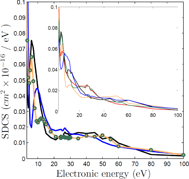
Figure 2: Single differential cross sections for the $p+H$ system as a function of the emitted electron energy, calculated at the different distances $Vt$ (in a. u.). The orange curve and the one described by green circles represent the energy distribution at $Vt=200$ a. u. calculated as described in the text, while the blue and black curves have a similar meaning for $Vt=50$ a. u. In the inset there are some energy distribution curves that sample the region occupied by the full set of distributions when the time dependent phase is varied through the distance $Vt$. The different colors red, orange, black, green and blue, correspond to $Vt$ of 100, 200, 300, 400 and 500 a. u.

In our study the distance interval $V\Delta t\sim 500$ a. u. corresponds to a time interval $\Delta t\sim 10^{-15}$ seconds that is close to the inverse of the difference between the lower pseudo-states energies. On the other hand, the data acquisition time in experimental runs is much more larger than this estimated time and for this reason the oscillations shown in Fig. 2 would not be seen in the experimental results. In order to compare with the experimental measurements, a key step in the present work is to make a temporal average of the calculated distributions for several $Vt$. This idea is discussed in the analysis of Fig. 3.

In Fig. 3 the black line shows results for the electron energy differential cross section for the $p+H$ system. That was calculated taking the time average of 40 distributions at different $Vt$ in the range of 100 to 550 a. u. In magenta circles is exhibited the experimental measurements obtained by Kerby et al. [20], whose uncertainties in their cross section are of 22 % above 10 eV, increasing to 26 % at 1.5 eV and to 50 % or more at the highest energies in the plot. What we have noticed in our calculation is that as we include more distributions in our time average, the mean distribution shows a smoother curve that approaches closer to the Kerby et al. experimental profile and the oscillatory character is pushed into lower energies. At energies above 20 eV, the differential cross section is larger than that shown experimentally and below 20 eV is lower than that.

Fig. 3 also shows other theoretical calculations using the approximation of the impact parameter. The results from Chassid et al. [11] (in blue line) fit well with the experimental data for high energies but has a significant disagreement at low energies. When our results are compared with those calculations, there is a significant difference in the shape of electron-energy differential cross sections. As we know from the introduction, both methods are similar in the main physical approximations and this is reflected in the good agreement in the ionization probability as a function of the impact parameter, as shown in the inset of Fig. 3. However the difference in the methods arises at the level of spectrum extraction as is pointed out in the introduction. One of these differences is that our calculation was done as an averaged distribution of several $Vt$’s in a range whose values are larger than the single $Vt$ value used by Chassid et al. where there is an important perturbation of the potential. Another difference is that we used the final wave function in the momentum space for obtaining the electron energy spectrum, whereas they got the energy spectrum by using eigenenergies of pseudostates in configuration space.

In the averaged distribution, the ECC structure diminishes considerably compared to that appearing in single distributions, as shown in Fig. 2. This little structure does not appear in the other theoretical calculations nor in the experimental data that indeed have not been measured at small angles and therefore it should not be there. A possible cause for missing the ECC peak in the work of Chassid et al. [11] could be that the $Vt$ distance used may not be sufficient to have the final electronic density profile for building the structure.The data calculated by Fu et al. [12]have a good agreement with experimental data but the ECC structure does not appear because a single center for pseudostates was considered.

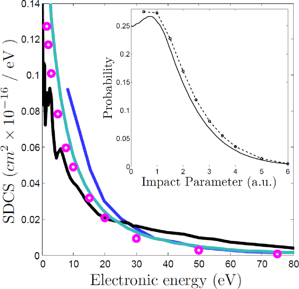
Figure 3: Ionization distribution in energy for the $p+H$ system at 50 keV. Black line shows the average distribution on time calculated in this work. Circles are the experimental data from Ref. [20], the turquoise line shows calculations from Ref. [12] and the blue line is theoretical data taken from Ref. [11]. In the inset, a comparison between our results and those of Chassid et al. [11] for the ionization probability as function of the impact parameter is shown.

The ionization cross section is presented in Fig. 4 for different $Vt$ distances in the region from 100 to 550 a. u. We can notice the oscillatory character of its behavior that arises from the time dependent phases that multiply the stationary atomic functions (see Eqs. 2, 3). The variation of the ionization cross section is roughly in the $1.6-1.75\times 10^{-16}$ $cm^{2}$ range and the time average of those values gives $1.68\times 10^{-16}$ $cm^{2}$. Some authors ([11, 23]) have identified this behavior and have suggested a time average procedure but have assumed that the average should be very close to their found solutions and have not proceeded to do further calculations.

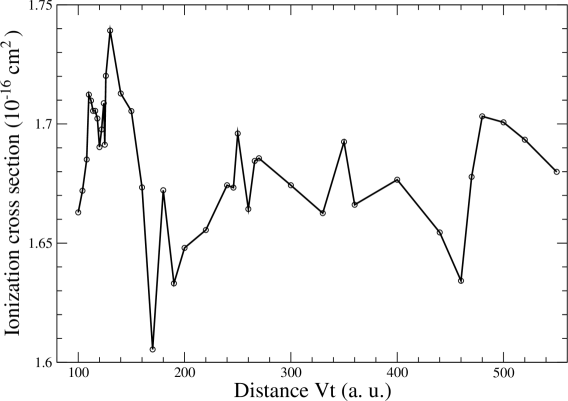
Figure 4: Ionization cross section for the $p+H$ system as a function of the distance $Vt$. The oscillations are due to the time dependent phases appearing in the atomic wave functions.

In Fig. 5 the electron-energy differential cross sections calculated at three incidents energies of 25, 50 and 100 keV and at single distance of $Vt=100$ a. u. are shown. The full lines represent calculations made with the differential probability in energy that includes the terms of interference between the two centers. The construction of the differential probability sometimes is done subtracting from the total wave function the projection of each set of functions, anchored at their respective center, on their own set of bound wave functions. The dashed lines represent calculations with probabilities obtained under this scheme. Both calculations differ by a neglectable amount that is not important when the time average is performed to make a comparison with experimental data, since this difference is much smaller than the distribution changes when several $Vt$ are used. Also the overlap has the tendency to diminish with a larger $Vt$. The main features of the distribution calculated at a projectile energy of 50 keV are also found at the other energies of 25 and 100 keV. Similar results are also found in $p+He$ system but are not shown in the manuscript.

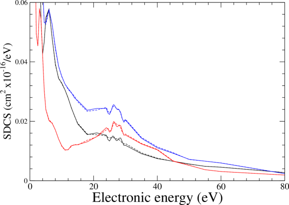
Figure 5: Ionization distribution in energy for the $p+H$ system at projectile energies of 25, 50 and 100 keV, at $Vt=100$ a. u., are represented in red, blue and black colors respectively. Full lines represent our results calculated with the coherent sum of the wave functions, and dashed lines, when overlaps between the two sets of wave functions anchored in each center are not included. We notice that the overlap is not important and therefore can be ignored.

The curves displayed in Fig. 6 are some energy distributions of ionized electrons in the $p+He$ collision calculated with the ionization function evaluated at different distances $Vt$, where the potential interaction does not affect the electronic distribution and then the variation of those distributions are due essentially to the time dependent phases. Similarly to hydrogen case, a more notorious structure is seen in the cusp electrons region for each calculated curve at a given $Vt$. After the temporal average is done, the structure maintains its presence there, as is shown in Fig. 7.

In Fig. 7, the single differential cross section as function of the energy of ejected electrons obtained in this work is compared with several experimental data and theoretical calculations reported in the literature for the $p+He$ system. We understand that experimental data have been normalized following different schemes and therefore is meaningful to compare only their distribution profiles with the one we got in this work.

For energies larger than 15 eV our calculation follows a path close to the experimental results, and below that energy there is a slope change in experimental data measured by Gibson [25] and Schulz [8], which is also seen in this work. In the data of reference [26] does not appear the structure close to 27 eV since the measurements were done at electron emission angles above $10\,^{\circ}$. Also, the theoretical curve reported by Gulyas (Ref. [8]) follows very close the measurements made by Cheng et al. For the energy range shown in Fig. 7, similarly to $p+H$, in the $p+He$ system the curve gets a smoother profile at large energies and the oscillations diminish at lower energies, as the number of distribution curves increases in the average calculation.

It is noted that in the cases of $H$ and $He$, the best theoretical agreement with experiment is achieved with various techniques [12, 11] and [8] respectively. In our case, the technique that is applied to the two reactions provides an acceptable agreement with experiments of both systems.

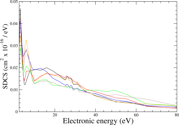
Figure 6: Single differential cross section for the $p+He$ system as a function of the emitted electrons energy, calculated at the different distances $Vt$’s of 100, 125, 150, 175, 190 and 200 a. u. The difference between the shapes of the curves are due to the phases that multiply the stationary atomic wave functions. A temporal average of the curves is necessary to compare the results with data reported in the literature (see Fig. 7).

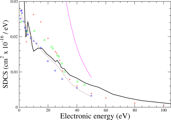
Figure 7: Ionization distribution in ejected electron energy for the $p+He$ system at 50 keV. For experimental data, the crosses shows data from Ref. [25], squares from Ref. [8] and diamonds from Ref. [8] (where is ascribed to [26]). For the theoretical calculations, the thin magenta line is Born+PCI calculations from Ref. [8], and the brown thin line is the CWD calculated by Gulyas (Ref. [8]). Considering 20 distributions, the temporal average result found in this work is given by the thick black line. It shows the general trend of experimental results above 15 eV.

5 Conclusions

In this paper the energy distributions of the ionized electrons for the $p+H$ and $p+He$ systems are calculated at 50 keV. The calculation is performed in the impact parameter approximation using the method of Close Coupling in two centers. The results obtained with this method are compared with previous calculations for these systems, obtained with similar methods. When a time average on the distributions at different distances $Vt$ is done, the agreement is reasonable with some of them and there is an improvement regarding others. It is also found that the averaged distribution has a betterment in the sense of becoming softer, and closer to the experimental results as more curves are included in the average calculation, which we believe is very important to achieve an agreement with experimental data especially at low electronic energies. This work is a systematic study that clarifies ambiguities in other studies regarding magnitudes of final internuclear distances to be taken into account in the calculation, as well as suggestions regarding unrealized temporal averages.

As an extension of this work the projectile angle may be incorporated to obtain double differential cross section, following the approach studied in Ref. [27]. We do not foresee major complications inherent to the method for applying this approach to more complex colliding systems.

Appendix

Fourier transform of atomic functions

We can obtain an explicit expression for the Fourier transform of atomic functions (Eq. 4) following Podolsky and Pauling [28]. In terms of spherical coordinates that equation can be written as:

$$\begin{array}[]{rl}\tilde{\phi}_{lm}\left(\mathbf{p}_{i}\right)&=h^{-3/2}\left(\frac{1}{2\pi}\right)^{1/2}\left[\frac{\left(2l+1\right)\left(l-m\right)!}{2\left(l+m\right)!}\right]^{1/2}{\displaystyle\sum_{k=1}^{k_{max}}}s_{nl}^{k}\left[\frac{\left(2\alpha_{l}\beta_{l}^{k}\right)^{2l+3}}{\left(2l+2\right)!}\right]^{1/2}\\ \\ &\times\int_{0}^{\infty}dr_{i}\,r_{i}^{l+2}e^{-\alpha_{l}\beta_{l}^{k}r_{i}}\int_{0}^{\pi}e^{-i\,\left(2\pi/h\right)r_{i}p_{i}\cos\theta_{i}\cos\vartheta_{i}}P_{l}^{m}(\cos\theta_{i})\sin\theta_{i}d\theta_{i}\\ \\ &\times\int_{0}^{2\pi}e^{\pm im\phi_{i}-i\,\left(2\pi/h\right)r_{i}p_{i}\sin\theta_{i}\sin\vartheta_{i}\cos\left(\varphi_{i}-\phi_{i}\right)}d\phi_{i},\end{array}$$ (13)

where $\left(p_{i},\vartheta_{i},\varphi_{i}\right)$ and $\left(r_{i},\theta_{i},\phi_{i}\right)$ denotes the momentum and spatial spherical polar coordinates respectively, and $h$ is the Planck constant. After the integrations over $\phi_{i}$ and $\theta_{i}$, Eq. 13 can be simplified as

$$\begin{array}[]{cl}\tilde{\phi}_{lm}\left(\mathbf{p}_{i}\right)&=h^{-3/2}\left(-2\pi\right)\left(-\mathfrak{i}\right)^{l}\left(\frac{h}{p_{i}}\right)^{1/2}\\ \\ &\times\left(\frac{1}{2\pi}\right)^{1/2}e^{\pm\mathfrak{i}m\varphi_{i}}\left[\frac{\left(2l+1\right)\left(l-m\right)!}{2\left(l+m\right)!}\right]^{1/2}P_{l}^{m}\left(\cos\vartheta_{i}\right)\\ \\ &\times{\displaystyle\sum_{k=1}^{k_{max}}}s_{nl}^{k}\left[\frac{\left(2\alpha_{l}\beta_{l}^{k}\right)^{2l+3}}{\left(2l+2\right)!}\right]^{1/2}\int_{0}^{\infty}dr_{i}\,r_{i}^{l+3/2}e^{-\alpha_{l}\beta_{l}^{k}r_{i}}J_{l+1/2}\left(\frac{2\pi rp_{i}}{h}\right).\end{array}$$ (14)

For the integral

$$I_{kl}\left(p\right)=\int_{0}^{\infty}dr\,r^{l+3/2}e^{-\alpha_{l}\beta_{l}^{k}r}J_{l+1/2}\left(\frac{2\pi rp}{h}\right),$$

an analytical expression can be obtained ([29], p712, eq. 6.623 2.):

$$I_{kl}\left(p\right)=\frac{2\alpha_{l}\beta_{l}^{k}\left(2\frac{2\pi p}{h}\right)^{l+1/2}\Gamma\left(l+2\right)}{\sqrt{\pi}\left(\left[\alpha_{l}\beta_{l}^{k}\right]^{2}+\left[\frac{2\pi p}{h}\right]^{2}\right)^{l+2}}.$$

Substituting this into Eq. $\left[\ref{eq:2A}\right]$, we obtain

$$\begin{array}[]{cl}\tilde{\phi}_{lm}\left(\mathbf{p}_{i}\right)&=-h^{-3/2}2\pi\left(-\mathfrak{i}\right)^{l}\left(\frac{h}{p_{i}}\right)^{1/2}Y_{lm}\left(\vartheta_{i},\varphi_{i}\right)\\ \\ &\times{\displaystyle\sum_{k=1}^{k_{max}}}s_{nl}^{k}\left[\frac{\left(2\alpha_{l}\beta_{l}^{k}\right)^{2l+3}}{\left(2l+2\right)!}\right]^{1/2}\frac{2\alpha_{l}\beta_{l}^{k}\left(2\frac{2\pi p_{i}}{h}\right)^{l+1/2}\Gamma\left(l+2\right)}{\sqrt{\pi}\left(\left[\alpha_{l}\beta_{l}^{k}\right]^{2}+\left[\frac{2\pi p_{i}}{h}\right]^{2}\right)^{l+2}},\end{array}$$ (15)

where $Y_{lm}\left(\vartheta_{i},\varphi_{i}\right)$ are the normalized spherical harmonics in momentum space. In atomic units, we can rewrite the previous equation as

$$\begin{array}[]{cl}\tilde{\phi}_{lm}\left(\mathbf{p}_{i}\right)&={\displaystyle\sum_{k=1}^{k_{max}}}s_{nl}^{k}\frac{-\left(-\mathfrak{i}\right)^{l}2^{2l+3}\left(\alpha_{l}\beta_{l}^{k}\right)^{l+5/2}\left(l+1\right)!}{\left[\pi\left(2l+2\right)!\right]^{1/2}}\frac{\left(p_{i}\right)^{l}}{\left(\left[\alpha_{l}\beta_{l}^{k}\right]^{2}+\left[p_{i}\right]^{2}\right)^{l+2}}Y_{lm}\left(\vartheta_{i},\varphi_{i}\right),\end{array}$$ (16)

that when compared to Eq. 5, defines the functions $F_{l}^{k}$.

Acknowledgments

This work was supported by the Dirección General de Asuntos del Personal Académico, UNAM, under project IN109511-3.

References

- [1] T. Kirchner and H. Knudsen, J. Phys. B: At. Mol. Phys. 44, 122001 (2011).
- [2] T. P. S. Sharma, B. R. Lamichhane, A. Hasan, J. Remolina, S. Gurung, L. Sarkadi and M. Schulz, J. Phys. B: At. Mol. Phys. 48, 175204 (2015).
- [3] F. Xiao-Ying, Z. Rui-Fang, D. Hui-Xiao, S. Shi-Yan and J. Xiang-Fu, Chin. Phys. B 23, 063404 (2014)
- [4] A. C. F. Santos, W. Wolff, M. M. Sant’Anna, G. M. Sigaud and R. D. DuBois, J. Phys. B: At. Mol. Opt. Phys. 46 075202 (2013).
- [5] M. E. Rudd, Y. -K. Kim, D. H. Madison and J. W. Gallagher, Rev. Mod. Phys. 57, 965 (1985).
- [6] N. Stolterfoth, R. D. DuBois and R. D. Rivarola, Electron emission in heavy ion-atom collisions, Springer series on atoms and plasmas, Springer, New York (1997).
- [7] S. Yu. Ovchinnikov, G. N. Ogurtsov, J. H. Macek and Yu. S. Godeev, Phys. Rep. 389, 189 (2004).
- [8] M. Schulz, A. Hasan, N. V. Maydanyuk, M. Foster, B. Tooke and D. H. Madison, Phys. Rev. A 73, 062704 (2006).
- [9] D. R. Schultz, C. O. Rienhold, P. S. Krstić and M. R. Strayer, Rev. A 65, 052722 (2002).
- [10] E. Y. Sidky and C. D. Lin, J. Phys. B: At. Mol. Phys. 31, 2949 (1998).
- [11] M. Chassid and M. Horbatsch, Phys. Rev. A 66, 012714 (2002).
- [12] J. Fu, M. J. Fitzpatrick, J. F. Reading, and R. Gayet, J. Phys. B: At. Mol. Phys. 34, 15 (2001).
- [13] J. F. Reading, J. Fu, and M. J. Fitzpatrick, Nucl. Instr. and Meth. B 241, (2005).
- [14] W. Fritsch and C. D. Lin, Phys. Rep. 20, 1 (1991).
- [15] J. F. Reading, A. L. Ford, G. L. Swafford and A. Fitchard, Phys. Rev. A 20, 130 (1979).
- [16] T. Spranger and T. Kirchner, J. Phys. B: At. Mol. Phys. 37, 4159 (2004).
- [17] T. G. Winter, Phys. Rev. A 80, 032701 (2009).
- [18] M. J. Fitzpatrick, J. Fu, W. F. Smith, J. F. Reading, A. Dubois and R. Gayet, Radiation Phys. and Chem. 76, 426 (2007).
- [19] G. W. McLure, Phy. Rev. 148, 47 (1966).
- [20] G. W. Kerby, M. W. Gealy, Y. -Y. Hsu, M. E. Rudd, D. R. Schultz and C. O. Reinhold, Phys. Rev. A 51, 2256 (1995).
- [21] N. Toshima, Phys. Rev. A 59, 1981 (1999).
- [22] A. Amaya-Tapia and A. Antillón, J. Phys. B, Conference Series 388, 082002 (2012).
- [23] E. Y. Sidky and C. D. Lin, Phys. Rev. A 60, 377 (1999).
- [24] T-G. Lee, S. Yu. Ovchinnikov, J. Stenberg, V. Chupryna, D. R. Schultz and J. H. Macek, Phys. Rev. A 76, 05701 (2007).
- [25] D. K. Gibson and I. D. Reid, J. Phys. B: At. Mol. Phys. 19, 3265 (1986).
- [26] W. Q. Cheng, M. E. Rudd and Y. Y. Hsu, Phys. Rev. A 39, 2359 (1989).
- [27] M. McGovern, D. Assafrão, J. R. Mohallem, Colm T. Whelan and H. R. J. Walters, Phys. Rev. A 79, 042707 (2009).
- [28] W. Q. Cheng, M. E. Rudd and Y. Y. Hsu, Phys. Rev. A 39, 2359 (1989). B. Podolsky and L. Pauling, Phys. Rev. 34, 109 (1929).
- [29] I. S. Gradshteyn and I. M. Ryzhik, Table of integrals, series and products, Academic Press, New York, (1965).