The Impact of Unlicensed Access on Small-Cell Resource Allocation

Abstract

Small cells deployed in licensed spectrum and unlicensed access via WiFi provide different ways of expanding wireless services to low mobility users. That reduces the demand for conventional macro-cellular networks, which are better suited for wide-area mobile coverage. The mix of these technologies seen in practice depends in part on the decisions made by wireless service providers that seek to maximize revenue, and allocations of licensed and unlicensed spectrum by regulators. To understand these interactions we present a model in which a service provider allocates available licensed spectrum across two separate bands, one for macro- and one for small-cells, in order to serve two types of users: mobile and fixed. We assume a service model in which the providers can charge a (different) price per unit rate for each type of service (macro- or small-cell); unlicensed access is free. With this setup we study how the addition of unlicensed spectrum affects prices and the optimal allocation of bandwidth across macro-/small-cells. We also characterize the optimal fraction of unlicensed spectrum when new bandwidth becomes available.

I Introduction

Current cellular networks are evolving towards heterogeneous networks (HetNets) to cope with the accelerating demand for wireless data along with variations in mobility and service requirements[1, 2]. The primary feature of a HetNet is the deployment of multiple types of access infrastructure with different transmission powers, range, and spectral efficiency, such as small-cells targeting local “hot spots.” In addition to cellular infrastructure in licensed spectrum allocations, unlicensed services (e.g., WiFi) are an increasingly common alternative for providing users local access. As unlicensed networks and HetNets proliferate, wireless users have greater choice in the type of network they can access. That can in turn affect strategic decisions on the part of the SPs regarding pricing and network resource allocation.

While the introduction of HetNets, and small-cell networks in particular, will increase overall data capacity, network management and resource allocation become more complicated. In particular, an SP must allocate available resources across different cell types (small vs macro) taking into account mobility patterns and demand for different services. That allocation then interacts with pricing strategies that can differentiate among service categories and controls revenue. Resource allocation is further complicated by the existence of unlicensed WiFi networks, which can be viewed both as an additional resource for offloading traffic, and as a source of competition for small-cell networks in licensed spectrum.

In this paper we study the effect of unlicensed spectrum on resource allocation in HetNets containing large- (macro-) and small- (pico- or femto-) cells. The macro- and small-cells are assumed to be operated by a cellular SP, or multiple competing SPs, using licensed (proprietary) spectrum. To model the demand for different services, we assume two types of users: mobile and fixed. The mobile users must be served by macro-cells only, whereas the fixed users can be served by either the macro- or small-cells, or via the unlicensed spectrum. We assume that the SPs charge a price per unit rate to access their network. The macro- and small-cells are viewed as providing two different services, hence the SPs set two corresponding prices for access. There is no access fee for the unlicensed band. In all cases the available rate is split among all users sharing the band. Given this setup, the SPs wish to set prices and allocate bandwidth across the macro- and small-cells to maximize their revenue.

Our model is similar to that presented in our previous work [14] to study bandwidth allocation in HetNets with competing SPs; however, here the main distinguishing feature is the presence of the unlicensed band. Our results show how the unlicensed spectrum affects the SPs’ willingness to allocate resources to the small-cell network. Moreover, the model and results can be used to quantify the utility (total welfare) offered by the unlicensed spectrum, and to compare it with that generated by the licensed spectrum taking the strategic decisions of the SPs into account. The introduction of unlicensed spectrum raises several analytical challenges vis-a-vis prior work (e.g., [14]). This is due to the expanded set of choices (i.e., for fixed-user association) and also the additional conditions on equilibria due to competition from the unlicensed service.

We now summarize our main results. We first focus on a monopoly SP, and then consider the more complicated scenario with multiple competing SPs. In all scenarios we model the SP and user actions as a two-stage game in which the SPs first partition the licensed band into subbands for the macro- and small-cell networks, and subsequently announce prices for services. The prices then enable the fixed users to determine their network association (macro-/small-/unlicensed). The following results are obtained by analyzing sub-game perfect equilibria, assuming a class of $\alpha$-fair utility functions for tractability.

1. HetNet Market structure: In equilibrium the macro-cell network serves only mobile users. Fixed users then associate with either the small-cell or unlicensed network. This applies when the SPs maximize either revenue or social welfare. Hence this association is optimal in the sense of maximizing social welfare.

2. Bandwidth allocation with monopoly SP: Comparing bandwidth allocations with and without unlicensed spectrum, when maximizing revenue, a monopoly SP may allocate more bandwidth to small-cells with unlicensed than without. This occurs when the unlicensed network offers a sufficiently low rate (e.g., due to a small amount of unlicensed bandwidth). This seems counterintuitive when the unlicensed network is viewed as an additional resource; however, this is because the presence of unlicensed bandwidth alters the dependence of quantity (users served) with price. In contrast, when the SP maximizes social welfare, it always allocates less bandwidth to small cells with unlicensed spectrum.

3. Equilibrium with competitive SPs: With multiple competitive SPs we prove that there always exists a unique sub-game perfect equilibrium with an associated bandwidth allocation. Furthermore, the equilibrium can fall in one of three categories: (1) all SPs allocate bandwidth to both macro- and small-cells (“Macro-Small Nash Equilibrium”, or MSNE); (2) a subset of SPs allocate bandwidth to macro-cells only, and the rest allocate to both macro and small cells (“Macro-Preferred Nash Equilibrium”, or MPNE); and (3) all SPs allocate bandwidth only to macro-cells (“Macro-only Nash Equilibrium”, or MNE). Without unlicensed spectrum for our choice of utility functions only the MSNE is possible [14]. Hence the increased competition from the unlicensed network may cause some SPs to give up on small-cells and allocate bandwidth only to the macro-cells. We also consider the asymptotic scenario where the number of SPs goes to infinity and observe that in general, the equilibrium with an arbitrary amount of unlicensed spectrum does not achieve the maximum social welfare.

4. Dependence of social welfare on the licensed/unlicensed split: For spectrum regulators, such as the FCC, a challenge is determining how much newly available spectrum should be licensed or unlicensed. We use our results to illustrate how the mix of licensed and unlicensed spectrum affects social welfare. This depends crucially on the relative spectral efficiencies associated with the small-cell and unlicensed networks. If the small-cell network has higher spectral efficiency, then allocating the entire bandwidth as licensed maximizes social welfare. Conversely, if the unlicensed network has higher spectral efficiency, then there is an optimal (positive) amount of unlicensed spectrum, which may or may not achieve the maximum social welfare. Furthermore, allocating insufficient unlicensed bandwidth in this scenario can cause the social welfare to decrease below the all-licensed allocation. (This is illustrated in Fig. 5 in Sec. VII.)

Related work on pricing and bandwidth allocation in heterogeneous wireless networks is presented in [3, 4, 5, 6, 7, 8, 9]. In [3, 4, 5] small-cell service is an enhancement to macro-cell service, and in [6, 7, 8, 9] small- and macro-cells provide separate services (as we assume here). Optimal pricing only is studied in [3, 5], whereas joint pricing and bandwidth allocation is studied in [4, 6, 7, 8, 9]. However, in that work there is a single SP (monopoly) and no unlicensed spectrum.

In [10, 11, 12, 13, 14], competition among multiple SPs providing HetNet services is investigated. References [10, 11] study pricing and service competition with fixed bandwidth allocations, while [12, 13, 14] study both pricing and bandwidth optimization. However, in [12, 13] the SPs compete to acquire the spectrum from a spectrum broker, as opposed to optimizing the bandwidth allocation across the different cell types in [14]. The preceding work does not consider any interactions with unlicensed access.

While the preceding work focuses on HetNet deployments using licensed spectrum, the interaction of unlicensed with licensed spectrum in other contexts is considered in [15, 16, 17]. In [15] an economic analysis of the trade-off between incremental licensed and unlicensed spectrum allocations is presented, which shows that licensed spectrum is the favored option. In [16], an intermediate model of price competition between two SPs having a fixed licensed part of the spectrum and sharing the remaining part as unlicensed is proposed. It is shown that user welfare increases with the proportion of unlicensed spectrum; however, the overall social welfare decreases, indicating resources are used less efficiently. Reference [17] studies social welfare when unlicensed spectrum is added to an existing allocation of licensed spectrum among incumbent competing SPs. The conclusion is that the social welfare can decrease over a significant range of unlicensed bandwidths. The preceding work assumes that the licensed spectrum supports a single type of service, hence does not consider the associated bandwidth allocation problem studied here. Also, except for [17], the users are assumed to be homogeneous.

The paper is organized as follows. We introduce our system model in Section II. The price and user association equilibrium for a monopoly SP is presented in Section III. Optimal bandwidth allocation for revenue maximization is discussed in Section IV, and for social welfare maximization in Section V. We then consider multiple competing SPs in Section VI. The dependence of social welfare on the amount of unlicensed bandwidth is discussed in VII, and conclusions are presented in Section VIII. All proofs of the main results and several supplemental results can be be found in the appendices.

II System Model

II-A Network Model

We consider a scenario where there are one or more SPs, each of which has a two-tier cellular network operating in licensed spectrum consisting of macro-cells (with wide coverage) and small-cells (with only local coverage). Macro-cells and small-cells are assumed to operate in separate bands. We also assume that there is unlicensed spectrum in which WiFi Access Points (APs) are deployed with no access charges. The assumption of no access charge is made to make the unlicensed as desirable as possible to the users. Users in the network are classified into two categories based on their mobility: mobile users that can only be served by macro-cells and fixed users that can be served by macro-cells, small-cells or WiFi (but not multiple at the same time).

Macro-cells, small-cells and WiFi APs are assumed to be uniformly deployed over a given area. To simplify our analysis we restrict our attention to the case where all SPs have the same infrastructure deployment density. The density of macro-cells per SP is normalized to one and we denote the densities of small-cells and WiFi APs by $N_{S}$ and $N_{U}$, respectively. Both types of users are also uniformly deployed over the given area, and we assume a large number of users so that we can model them as non-atomic. The density of fixed and mobile users are given by $N_{f}$ and $N_{m}$, respectively.

We assume that each SP $i$ has total bandwidth $B_{i}$ and the macro-cells of SP $i$ can provide a total data rate of $C_{i,M}=B_{i,M}R_{0}$, where $R_{0}$ is the (average) spectral efficiency and $B_{i,M}$ is the bandwidth allocated to macro-cells by SP $i$. Similarly, the total available rate in small-cells of SP $i$ and in WiFi APs are defined as $C_{i,S}=\lambda_{S}B_{i,S}R_{0}$ and $C_{U}=\lambda_{U}B_{U}R_{0}$, respectively. Here $\lambda_{S}$ and $\lambda_{U}$ reflect the rate difference due to the combination of spectral efficiency and deployment density differences in small-cells and WiFi APs compared with macro-cells. Since small-cells generally have a higher spectral efficiency and larger deployment density, we assume $\lambda_{S}>1$. WiFi APs typically have a higher deployment density but lower spectral efficiency. Therefore, we don’t make any assumptions on $\lambda_{U}$.

II-B Market Model

Each SP $i$ offers separate macro- and small- cell service. It charges all users of a given service the same price per unit rate, which are denoted by $p_{i,M}$ and $p_{i,S}$ for macro- and small- cell service of provider $i$, respectively. Of course, other pricing approaches arise in practice such as flat-rate pricing. We focus on per unit pricing in part because it is analytically tractable and in part because, as will be shown in our analysis, it is sufficient for optimizing the total user welfare. Recall, WiFi service is assumed to have no access charge.

The density of users connected to macro-cells and small-cells of SP $i$ and to WiFi are denoted by $K_{i,M}$, $K_{i,S}$ and $K_{U}$, respectively. Note that $K_{i,S}$ and $K_{U}$ only consist of fixed users, while $K_{i,M}$ may include both mobile users and fixed users. Additionally, mobile users are assumed to have priority connecting to macro-cells. As a result, macro-cells can only accommodate fixed users if all mobile users have been served.

II-C User Optimization

Each user is endowed with a utility function $u(r)$, which only depends on the service rate it gets from any type of service. For simplicity of analysis, we assume that all users have the same utility and we further restrict this to be an $\alpha$-fair utility functions [19] with $\alpha\in(0,1)$:

$$u(r)=\frac{r^{1-\alpha}}{1-\alpha},\quad\alpha\in(0,1).$$ (1)

This restriction enables us to explicitly calculate many equilibrium quantities, which appears to be difficult for more general classes of utility. Further this class is widely used in both networking and economics, where it is a subset of the class of iso-elastic utility functions.

For a given licensed service, each user requests a rate that maximizes their net payoff $W$, defined as the difference between their utility and the cost of service, i.e. they solve:

$$\underset{r\geq 0}{\text{maximize}}\quad W=u(r)-pr,$$ (2)

where as described below, the SPs will set the prices $p$ to ensure that the resulting demand can be met. For WiFi service, since there is no access charge, we assume all users simply share the available total rate equally. Since fixed users can choose any one service, they would choose the one with the largest payoff.

For $\alpha$-fair utility functions, (2) has the unique solution:

$$r^{*}=D(p)=(u^{\prime})^{-1}(p)=(1/p)^{1/\alpha},$$ (3)

where $D(p)$ is the user’s rate demand function and $u^{\prime}$ denotes the first derivative of $u$. The maximum net payoff for a user is thus:

$$W^{*}(p)=u(D(p))-pD(p)=\frac{\alpha}{1-\alpha}p^{1-\frac{1}{\alpha}}.$$ (4)

II-D Service Provider Optimization

Each SP $i$ needs to decide on the bandwidth partition $(B_{i,M},B_{i,S})$ and pricing decisions $(p_{i,M},p_{i,S})$ to maximize its revenue $S_{i}$, i.e., the aggregate amount paid by all users choosing its macro- and small- cell services. This can be formulated as:

maximize $$S_{i}=K_{i,M}p_{i,M}D(p_{i,M})+K_{i,S}p_{i,S}D(p_{i,S})$$

subject to $$K_{i,M}D(p_{i,M})\leq C_{i,M},K_{i,S}D(p_{i,S})\leq C_{i,S}$$

$$0\leq p_{i,M},p_{i,S}<\infty$$

$$B_{i,M},B_{i,S}\geq 0,B_{i,M}+B_{i,S}\leq B_{i}.$$ (5)

Here the first constraint ensures that the SP can meet the rate demanded by the users, where recall $C_{i,M}$ and $C_{i,S}$ depend on the bandwidth allocation. Note also that $K_{i,M}$ and $K_{i,S}$ will depend on the users associations, which in the case of multiple SPs will depend on the prices and bandwidths chosen by those SPs. Hence, we model the choice of bandwidth allocations and prices as a game played among the SPs. In practice, since bandwidth allocation takes place over a slower time-scale than price adjustments, we view this game as consisting of the following two stages: First, SPs determine their bandwidth allocation between macro-cells and small-cells. Then given their bandwidth allocation, SPs announce prices for both macro- and small-cells. Users then choose the services accordingly based on our association rules.

For such a game we characterize its sub-game perfect equilibrium by first characterizing a user association equilibrium in which SPs set prices given a fixed bandwidth allocation and then study the equilibrium bandwidth allocation based on the results obtained in the first step.

We also consider the choice of bandwidth allocations and prices that maximize the social welfare, i.e. the sum utility over all users. This can be formulated as maximizing

$$\text{SW}=\sum\limits_{i=1}^{N}K_{i,M}u(R_{i,M})+K_{i,S}u(R_{i,S})+K_{U}u(R_{U})$$ (6)

subject to the same constraints for each SP $i$ as in (II-D). Here, $R_{i,M}$, $R_{i,S}$ and $R_{U}$ denote the average service rates per user in each respective service, which in turn depends on the prices and bandwidth allocations.

III User Association with a Single SP

In this section we study the user association equilibrium given a fixed bandwidth allocation between macro- and small-cells by a single SP. Here we assume the SP maximizes revenue, and consider social welfare maximization in Section V. Since mobile users can only connect to macro-cells, we need only consider the association of fixed users.

Given a fixed bandwidth allocation and annoucned prices, users select their service to maximize their net payoff. For macro- and small-cell service the net payoff for a user is given by (4). Since $W^{*}(p)$ is a decreasing function of $p$, the choice between macro- and small-cell networks, ignoring the unlicensed network, is simply the one with the lower price. For the WiFi service, the users net payoff is simply given by $u(\frac{C_{U}}{K_{U}})$. With non-atomic users, it follows that in any user association equilibrium the net payoffs of any services that are used by fixed users must be equal, and any service not used must have a lower net payoff.

The SP adjusts the prices $p_{M}$ and $p_{S}$ to maximize its revenue taking into account the user association equilibrium. Two scenarios are possible:
1. Mixed service: Macro-cells serve both mobile users and a subset of fixed users;
2. Separate service: Macro-cells only serve mobile users.

Theorem 1 (User Association)

Given a fixed bandwidth allocation between macro- and small-cells, at the SPs’ optimal prices, the market clears, i.e., all users are served, and all rate is allocated. Further, there exists a threshold $B_{S,0}$ such that if $B_{S}<B_{S,0}$, then the mixed service scenario holds. Otherwise, the separate service scenario holds.

For the mixed service scenario, $p_{M}=p_{S}$, whereas for the separate service scenario $p_{M}>p_{S}$.

Hence, fixed users choose to associate with macro-cells only when the small-cell bandwidth is sufficiently small. In equilibrium the mixed service scenario implies that the net payoff to fixed users from connecting to macro-, small-cells and WiFi must be the same, and so we can write

$$\begin{split}u\Big{(}\frac{C_{S}}{K_{S}}\Big{)}-p_{S}\frac{C_{S}}{K_{S}}&=u\Big{(}\frac{C_{U}}{K_{U}}\Big{)}=u\Big{(}\frac{C_{M}}{K_{M}}\Big{)}-p_{M}\frac{C_{M}}{K_{M}},\end{split}$$ (7)

Note here we are using the fact from Theorem 1 that all of the rate is allocated. For separate service the same equality will hold except only for small-cells and unlicensed. With $\alpha$-fair utilities, the rate per user $\frac{C_{S}}{K_{S}}$ must satisfy (3). Using this in the above equations yields the following lemma that gives a useful comparison of the equilibrium rates of each service.

Lemma 1

In equilibrium fixed users in licensed spectrum (macro-/small-cells) achieve $\frac{1}{\kappa}$ times the average rate of users in unlicensed spectrum where $\kappa=\alpha^{1/(1-\alpha)}$.

Note that $1/\kappa>1$, which accounts for the access price charged in licensed spectrum. Interestingly with $\alpha$-fair utilities this ratio is independent of any system parameters.

Using this quantity $\kappa$ we can express the bandwidth threshold in Theorem 1 as

$$B_{S,0}=\max\left({\kappa N_{f}B_{M}R_{0}-N_{m}C_{U},0}\right)/({\kappa N_{m}\lambda_{S}R_{0}}).$$ (8)

From Theorem 1, since all users are served we have $K_{U}+K_{S}+K_{M}=N_{m}+N_{f}$. Using this and Lemma 1, we have the following explicit expressions for the equilibrium densities of users for each type of service in the mixed service scenario:

$$\begin{split}K_{U}&=(N_{f}+N_{m})\frac{C_{U}}{C_{U}+\kappa(C_{M}+C_{S})},\\ K_{M}&=(N_{f}+N_{m})\frac{\kappa C_{M}}{C_{U}+\kappa(C_{M}+C_{S})},\\ K_{S}&=(N_{f}+N_{m})\frac{\kappa C_{S}}{C_{U}+\kappa(C_{M}+C_{S})}.\end{split}$$ (9)

Similarly, for the separate service scenario, we have:

$$\begin{split}K_{M}&=N_{m},\quad K_{S}=N_{f}\frac{\kappa C_{S}}{\kappa C_{S}+C_{U}},\\ K_{U}&=N_{f}\frac{C_{U}}{\kappa C_{S}+C_{U}}.\end{split}$$ (10)

IV Bandwidth Allocation with a Single SP

We now consider optimal bandwidth allocation given the prices and user association equilibrium in the preceding section. In the mixed service scenario, this is given by:

maximize $$S=(B_{M}+\lambda_{S}B_{S})R_{0}u^{{}^{\prime}}\Big{(}\frac{(B_{M}+\lambda_{S}B_{S})R_{0}}{K_{M}+K_{S}}\Big{)}$$

subject to $$B_{M},B_{S}\geq 0,B_{M}+B_{S}\leq B,B_{S}<B_{S,0}.$$

where the objective is revenue, $K_{M},K_{S}$ are given in (9), and $B_{S,0}$ is defined in (8).

In the separate service scenario, the objective becomes

$$S=B_{M}R_{0}u^{{}^{\prime}}\Big{(}\frac{B_{M}R_{0}}{K_{M}}\Big{)}+\lambda_{S}B_{S}R_{0}u^{{}^{\prime}}\Big{(}\frac{\lambda_{S}B_{S}R_{0}}{K_{S}}\Big{)}$$ (11)

where $K_{M},K_{S}$ are given in (10), and the constraint $B_{S}\geq B_{S,0}$ applies.

Theorem 2 (Monopoly Bandwidth Allocation)

The optimal bandwidth allocation is unique and always corresponds to the separate service scenario.

The optimal bandwidth allocation $(B_{S}^{\text{rev}},B_{M}^{\text{rev}})$ can be determined by solving the necessary conditions given in Appendix B. Although the solution must be computed numerically, some general properties are easily established. First, $B_{M}^{\text{rev}}>0$ (always), but $B_{S}^{\text{rev}}>0$ if and only if $C_{U}<C_{U}^{\text{rev}}$ (otherwise $B_{S}^{\text{rev}}=0$), where

$$C_{U}^{\text{rev}}=\frac{\kappa N_{f}BR_{0}}{N_{m}}\Big{(}\frac{\lambda_{S}}{1-\alpha}\Big{)}^{\frac{1}{\alpha}}.$$ (12)

When $\alpha\rightarrow 0^{+}$ or $\alpha\rightarrow 1^{-}$, $C_{U}^{\text{rev}}\rightarrow+\infty$. That is, as the utility function becomes either linear or logarithmic, the SP always allocates some bandwidth to small-cells.

The optimal bandwidth allocation with no unlicensed spectrum can be determined by setting $C_{U}=0$. We will denote all associated quantities with a tilde, i.e., $(\tilde{B}_{S}^{\text{rev}},\tilde{B}_{M}^{\text{rev}})$ is the optimized bandwidth with $C_{U}=0$. With no unlicensed spectrum, it is straightforward to show that $\tilde{B}_{S}^{\text{rev}}=\tilde{\beta}B$ where $\tilde{\beta}=\tfrac{N_{f}}{N_{f}+N_{m}\lambda_{S}^{1-1/\alpha}}$, so that $\tilde{B}_{S}^{\text{rev}}>0$ and $\tilde{B}_{M}^{\text{rev}}>0$. In contrast, with unlicensed spectrum the additional competition can cause a revenue-maximizing SP to abandon small-cells altogether. We will see a more drastic example of this effect when we consider competing SPs.

The next theorem compares the amount of bandwidth allocated to small-cells with and without unlicensed spectrum.

Theorem 3 (Bandwidth Allocation Comparison)

There exists a threshold $C_{U}^{th}$ such that when $C_{U}<C_{U}^{th}$, $B_{S}^{\text{rev}}>\tilde{B}_{S}^{\text{rev}}$, and when $C_{U}>C_{U}^{th}$, $B_{S}^{\text{rev}}<\tilde{B}_{S}^{\text{rev}}$, where   $C_{U}^{th}=\beta^{*}\kappa\lambda_{S}\tilde{B}_{S}^{\text{rev}}R_{0}$ with $\beta^{*}$ being the unique strictly positive solution of

$$(1-\alpha)(1+\beta)^{1+\alpha}-\beta=1-\alpha.$$ (13)

Furthermore, the SP’s revenue is always less with unlicensed spectrum than without.

The last part of Theorem 3 is expected since unlicensed access competes with the SP for fixed users. The first part can be explained as follows. Compared to the case without unlicensed spectrum, when unlicensed spectrum is present if the SP keeps its bandwidth allocation the same, then it will clearly lose revenue as fewer users will use its small-cell service. To improve its revenue it could decrease $B_{S}$, shifting more resources to mobile users to make more revenue from them or it could increase $B_{S}$ to make its small-cell service more attractive and try to win back some users from the unlicensed network. However, increasing $B_{S}$ also results in a decrease in $p_{S}$ since the service rate per user increases (and a loss in revenue from the mobile users). When $C_{U}$ is small, this decrease in $p_{S}$ is smaller since more users will switch to the small-cells making the second option more attractive. When $C_{U}$ is large enough, fewer users will switch to the small-cells per unit of additional bandwidth, making the first option more profitable.

When $\alpha\rightarrow 0^{+}$, $\kappa\rightarrow 0^{+}$ (so that $\alpha$-fair utility function becomes the linear utility function), $\beta^{*}\rightarrow 0^{+}$, and therefore, $C_{U}^{th}\rightarrow 0^{+}$. This implies that the SP should always invest less bandwidth to small-cells compared with the scenario without unlicensed spectrum. However, in this case the SP should still invest almost all bandwidth to small-cells, i.e., $B_{S}^{\text{rev}}\rightarrow B$. This is because $\alpha=0$ effectively corresponds to maximizing the sum rate. (This can be seen directly from the revenue function.)

When $\alpha\rightarrow 1^{-}$, the utility function becomes logarithmic, $\kappa\rightarrow\mathrm{e}^{-1}$, and $\beta^{*}\rightarrow\infty$, so that $C_{U}^{th}\rightarrow\infty$. Hence, the SP should allocate more bandwidth to small-cells with unlicensed spectrum. Again, in the limit the SP allocates all bandwidth to small-cells, i.e., $B_{S}^{\text{rev}}\rightarrow B$. We can see this by rewriting the revenue function as follows:

$$S =B_{M}R_{0}u^{{}^{\prime}}\Big{(}\frac{B_{M}R_{0}}{K_{M}}\Big{)}+\lambda_{S}B_{S}R_{0}u^{{}^{\prime}}\Big{(}\frac{\lambda_{S}B_{S}R_{0}}{K_{S}}\Big{)}$$

$$=K_{M}R_{M}u^{{}^{\prime}}(R_{M})+K_{S}R_{S}u^{{}^{\prime}}(R_{S}).$$ (14)

For a log-utility function the revenue per mobile user $R_{M}u^{{}^{\prime}}(R_{M})$ and revenue per fixed user $R_{S}u^{{}^{\prime}}(R_{S})$ become constants and are equal. Therefore maximizing revenue is equivalent to maximizing $K_{M}$ and $K_{S}$. As a result, the SP allocates an arbitrarily small amount of bandwidth to the macro-cells to guarantee that all mobile users are served, and the remaining bandwidth to small-cells to maximize $K_{S}$. In contrast, with no unlicensed access $\tilde{\beta}$ converges to $\tfrac{N_{f}}{N_{f}+N_{m}}<1$ and $\lim_{\alpha\rightarrow 1^{-}}\tilde{B}_{S}^{\text{rev}}<B$.

V Social Welfare Maximization

Now we change the objective function to social welfare and analyze the corresponding prices, user association equilibrium and bandwidth allocation.

Theorem 4 (Social Welfare Maximization)

Given a single social welfare maximizing SP, in equilibrium we have the following properties:
1. The prices and user association are the same as for revenue maximization stated in Theorem 1.
2. The optimal bandwidth allocation is unique and corresponds to separate service.
3. Compared to the scenario without unlicensed spectrum, with unlicensed spectrum the SP always allocates less bandwidth to small-cells and more bandwidth to macro-cells.

Similar with revenue maximization, the optimal bandwidth allocation $(B_{S}^{\text{sw}},B_{M}^{\text{sw}})$ can be determined by solving the necessary conditions given in Appendix D. Also, it can be shown that $B_{M}^{\text{sw}}>0$ (always), and $B_{S}^{\text{sw}}>0$ if and only if $C_{U}<C_{U}^{\text{sw}}$ (otherwise $B_{S}=0$), where

$$C_{U}^{\text{sw}}=\frac{\kappa N_{f}BR_{0}\big{[}(\alpha+1)\lambda_{S}\big{]}^{\frac{1}{\alpha}}}{N_{m}}.$$ (15)

As $\alpha\rightarrow 0$, $C_{U}^{\text{sw}}\rightarrow+\infty$, i.e., in the limiting case of a linear utility function, the SP always allocates some bandwidth to small-cells, even if $C_{U}$ is large. Similar with revenue maximization, this is because this maximizes the total rate. When $\alpha\rightarrow 1$, $C_{U}^{\text{sw}}\rightarrow 2\mathrm{e}^{-1}\lambda_{S}\frac{N_{f}BR_{0}}{N_{m}}$ (as opposed to infinity for revenue maximization). With no unlicensed spectrum, $\tilde{B}_{S}^{\text{sw}}>0$ and $\tilde{B}_{M}^{\text{sw}}>0$.

Part 3) in Theorem 4 is due to the additional resources in the unlicensed network. Since fixed users are better off with unlicensed spectrum, to maximize the sum utility over all users, the SP allocates more bandwidth to the macro-cells.

We emphasize that with unlicensed spectrum, Theorems 3 and 4 imply that the optimal bandwidth allocation is different for revenue and social welfare maximization. That is, the corresponding necessary conditions generally have different solutions. In contrast, without unlicensed access, revenue and social welfare maximization give the same bandwidth allocation for $\alpha$-fair utility functions shown in our previous work[9].

Figure 1 shows an example of the optimal bandwidth allocation for different $\alpha$’s as the rate offered by the unlicensed network increases. Curves are shown for both revenue and social welfare maximization. The system parameters are $N_{f}=N_{m}=50$, $R_{0}=50$, and $\lambda_{S}=4$. For revenue maximization, the curve initially increases for small $C_{U}$, and then decreases. In contrast, for social welfare maximization, the curve is monotonically decreasing.

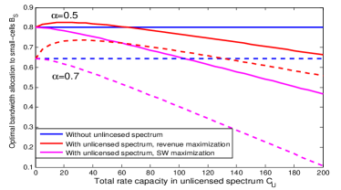
Figure 1: Optimal bandwidth allocation to small-cells for a single SP versus total unlicensed capacity.

VI Service Competition Among Multiple SPs

In this section we study service competition among $N>1$ SPs and investigate the corresponding sub-game perfect equilibrium with unlicensed spectrum. Users choose the service (macro-/small-/unlicensed) which yields the largest net payoff, and they fill the corresponding capacity accordingly. In licensed spectrum, if multiple services offer the same price, then the users are allocated across them in proportion to the capacities. Once a particular service’s capacity is exhausted, then the leftover demand continues to fill the remaining services in the same fashion. In unlicensed spectrum, fixed users always get an average rate equal to the total rate divided by the mass of fixed users associated with that network.

We again consider a sub-game perfect Nash equilibrium consisting of (i) A price equilibrium given a fixed bandwidth allocation; and (ii) An optimized bandwidth allocation given that prices are set according to (i). As for the scenario with a single SP, given a set of prices and bandwidth allocations, the user association equilibrium falls in one of two categories: a mixed service equilibrium in which all macro-cells serve both mobile and a subset of fixed users, and separate service equilibrium in which the macro-cells serve only mobile users. The next theorem generalizes Theorem 1 to multiple SPs.

Theorem 5 (Price Equilibrium with Multiple SPs)

Given fixed bandwidth allocations for all SPs, there is a unique price equilibrium which clears the market. Further if

$$\sum\limits_{i=1}^{N}B_{i,S}<\frac{\max\left(\kappa N_{f}\sum\limits_{i=1}^{N}B_{i,M}R_{0}-N_{m}C_{U},0\right)}{\kappa N_{m}\lambda_{S}R_{0}}$$

then a mixed service equilibrium holds. Otherwise, the separate service equilibrium holds.

For the mixed service scenario, $p_{i,M}=p_{i,S}$ for each SP $i$; in the separate service case, all SPs $i$ charge the same $p_{i,M}$ and $p_{i,S}$, with $p_{i,M}>p_{i,S}$.

The next theorem characterizes the equilibrium for the bandwidth allocation stage and thus the overall sub-game perfect Nash equilibrium for the game. Before stating this we define the following types of equilibria: A Macro-Small Nash Equilibrium (MSNE) is one where all SPs allocate bandwidth to both macro- and small-cells. A Macro-Preferred Nash Equilibrium (MPNE) is one where some SPs allocate bandwidth to both macro- and small-cells and the remaining SPs allocate bandwidth to macro-cells only. Finally, a Macro-only Nash Equilibrium (MNE) is one where all SPs allocate bandwidth to macro-cells only.

Theorem 6 (Nash Equilibrium)

There always exists a unique sub-game perfect Nash equilibrium and it corresponds to the separate service scenario. In the equilibrium fixed users in small-cells achieve a higher average rate than mobile users in macro-cells. Moreover, this Nash equilibrium can only be one of the following types: an MSNE, an MPNE or an MNE.

If there is no unlicensed spectrum, then for the $\alpha$-fair utility function only an MSNE exists and it is always efficient, i.e., maximizes social welfare [14]. Here, the presence of unlicensed access can cause a subset of the SPs to engage in macro-service only. Further, for any number of SPs, it can be shown that, in general, none of the equilibrium categories (including MSNE) are efficient. Figure 2 illustrates the Nash equilibrium regions for two SPs as a function of the available bandwidths $B_{1}$ and $B_{2}$. When $B_{1}$ and $B_{2}$ are sufficiently large, then the equilibrium is an MSNE, whereas if $B_{1}$ and/or $B_{2}$ become sufficiently small, the equilibrium transitions so that at least one SP serves only mobile users.

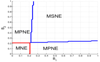
Figure 2: Nash equilibrium regions for 2 SPs. The system parameters are $\alpha=0.5,N_{m}=N_{f}=50,R_{0}=50,\lambda_{S}=4,\lambda_{W}=3,B_{U}=1$.

Proposition 1 (MSNE Properties)

Assuming an MSNE, for any two SPs $i$ and $j$ with total bandwidth $B_{i}$ and $B_{j}$, the following properties hold:
1) Symmetry: If $B_{i}=B_{j}$, then each SP’s bandwidth allocation must be the same, i.e., $B_{i,S}=B_{j,S},B_{i,M}=B_{j,M}$.
2) Monotonicity: If $B_{i}>B_{j}$, then SP $i$ allocates more bandwidth to both macro- and small-cells than SP $j$, i.e., $B_{i,S}>B_{j,S},B_{i,M}>B_{j,M}$.

Denote the total bandwidth allocated to small-cells by all SPs with and without unlicensed spectrum as $B_{S}$ and $\tilde{B_{S}}$, respectively.

Proposition 2 (MSNE Bandwidth Comparison)

If an MSNE exists with unlicensed access, then $B_{S}<\tilde{B_{S}}$.

Hence, for the MSNE case, competing SPs reduce the bandwidth allocation to small-cells when unlicensed spectrum is introduced.

Proposition 3 (MNE Conditions)

An MNE holds if and only if

$$C_{U}\geq\frac{R_{0}\sum_{i=1}^{N}B_{i}}{\big{(}1-\alpha\frac{B_{\max}}{\sum_{i=1}^{N}B_{i}}\big{)}^{\frac{1}{\alpha}}}\frac{\kappa N_{f}\lambda_{S}^{\frac{1}{\alpha}}}{N_{m}},$$ (16)

where $B_{\max}=\max\{B_{i}:i\in\mathcal{N}\}$.

For $N=1$ (monopoly) this condition yields the threshold in (12) so that the SP allocates no bandwidth to small-cells.

VII Unlicensed Bandwidth and Social Welfare

In this section we study the effect of increasing unlicensed bandwidth on social welfare. Using the preceding framework, we can determine the specific mix of unlicensed/licensed spectrum such that the market equilibrium yields the same social welfare as that achieved by a social planner. This is motivated by the scenario in which a spectrum regulator, such as the FCC, must determine how much newly available spectrum will be licensed or unlicensed. We assume a total available bandwidth $B$ and consider the following scenarios:

1) Efficient allocation: A social planner determines the bandwidth allocation to macro-cells $B_{M}$, small-cells $B_{S}$, and unlicensed network $B_{U}$ that maximizes total utility. We will denote the optimal allocation as $B_{M}^{\text{opt}},B_{S}^{\text{opt}},B_{U}^{\text{opt}}$, and use the corresponding social welfare as a benchmark.

2) Market equilibrium: Here a social planner determines the bandwidth assigned to licensed spectrum $B_{L}$ and unlicensed spectrum $B_{U}$. Each of the $N$ SPs operating in licensed spectrum obtains the same portion of total bandwidth $B_{i}\equiv\tfrac{B_{L}}{N}$, and then further determines the split of $B_{i}$ between $B_{i_{M}}$ and $B_{i_{S}}$ to maximize its revenue. This scenario corresponds to the more practical setting in which the regulator sets aside part of the available bandwidth as unlicensed, and grants licenses for the remainder. We will denote the bandwidths that maximize social welfare in this scenario as $B_{L}^{*},B_{U}^{*}$.

In the first scenario the social planner determines the bandwidth assignment without explicit pricing. The optimal bandwidth allocation equalizes the marginal utility for mobile and fixed users. It is easy to verify that the efficient allocation corresponds to separate service. In the market equilibrium scenario, we will use the results from Sections IV and VI to determine the optimal bandwidth assignments. We will also present social welfare curves for the asymptotic regime of many SPs, i.e., as $N\rightarrow\infty$, for which we will use the characterization below (full version in Appendix G).

Proposition 4

If we have

$$B_{U}\lambda_{U}>B\frac{\kappa N_{f}\lambda_{S}^{\frac{1}{\alpha}}}{N_{m}},$$ (17)

then there exists an $N^{*}(B_{U}\lambda_{U})$ such that for all $N>N^{*}(B_{U}\lambda_{U})$ we have an MNE. Otherwise, we always have an MSNE ($B_{i,M}>0$ and $B_{i,S}>0$ $\forall$ $i\in\mathcal{N}$, and $\forall$ $N$).

Given newly available bandwidth $B$, the optimal split into licensed and unlicensed subbands depends on the relative values of $\lambda_{S}$ and $\lambda_{U}$ (proofs in Appendix I). We have the following cases:
a) $\lambda_{S}>\lambda_{U}$: In this case an efficient allocation by a social planner would assign all spectrum to macro- and small-cells, i.e., there is no unlicensed network. The optimal bandwidth assignment is then:

$$B_{M}^{\text{opt}}=\frac{N_{m}B}{N_{m}+\mu_{S}N_{f}},B_{S}^{\text{opt}}=\frac{\mu_{S}N_{f}B}{N_{m}+\mu_{S}N_{f}},B_{U}^{\text{opt}}=0,\\$$ (18)

where $\mu_{S}:=\lambda_{S}^{\frac{1}{\alpha}-1}$. This is also true for the market equilibrium since it is shown in [9, 14] that without unlicensed spectrum, maximizing revenue is the same as maximizing social welfare for $\alpha$-fair utility functions, independent of $N$. Hence in this case the market equilibrium achieves the efficient allocation.

b) $\lambda_{S}=\lambda_{U}$: In this case the social planner only needs to consider the bandwidth assigned to macro-cells; the bandwidth split between small-cells and unlicensed access can be arbitrary. Here the optimal assignment satisfies

$$B_{M}^{\text{opt}}=\frac{N_{m}B}{N_{m}+\mu_{S}N_{f}},B_{S}^{\text{opt}}+B_{U}^{\text{opt}}=\frac{\mu_{S}N_{f}B}{N_{m}+\mu_{S}N_{f}},$$ (19)

where $\mu_{S}=\lambda^{\frac{1}{\alpha}-1}$. This includes the two extremes $(B_{S}^{\text{opt}}>0,B_{U}^{\text{opt}}=0)$ and $(B_{S}^{\text{opt}}=0,B_{U}^{\text{opt}}>0)$. Hence for the market equilibrium case, an optimal bandwidth assignment strategy is to allocate all bandwidth as licensed. As in case a), this achieves the efficient allocation. However, here there may exist another efficient allocation in which the fixed users are served by the unlicensed network. For the competing SPs, that corresponds to an MNE, i.e., the SPs only allocate their licensed bandwidth to the macro-cells ($B_{i,S}=0$ for all $i\in\mathcal{N}$).

The bandwidth allocation corresponding to this second optimal assignment, along with the condition for its existence, is

$$B_{L}^{*}=\frac{N_{m}B}{N_{m}+\mu_{S}N_{f}},B_{U}^{*}=\frac{\mu_{S}N_{f}B}{N_{m}+\mu_{S}N_{f}},$$

$$\qquad\text{if }N\geq 2\text{ or }N=1\text{ and }0<\alpha\leq 0.5.$$

For $N=1$, if $\alpha\in(0.5,1)$, then this second optimal point does not exist and the unique optimal bandwidth allocation corresponds to no unlicensed spectrum. All other bandwidth assignments yield lower social welfare.

c) $\lambda_{S}<\lambda_{U}$: In this case a social planner assigns spectrum to the macro-cell and unlicensed networks only; there is no small-cell network. The optimal allocation is:

$$B_{M}^{\text{opt}}=\frac{N_{m}B}{N_{m}+\mu_{U}N_{f}},B_{S}^{\text{opt}}=0,B_{U}^{\text{opt}}=\frac{\mu_{U}N_{f}B}{N_{m}+\mu_{U}N_{f}},\\$$ (20)

where $\mu_{U}=\lambda_{U}^{\frac{1}{\alpha}-1}$. For the market equilibrium, allocating all bandwidth to licensed spectrum no longer achieves the efficient allocation. The only possibility for achieving an efficient allocation, then, is to allocate $B_{U}^{\text{opt}}$ to unlicensed access. This achieves the efficient allocation if and only if the corresponding equilibrium is an MNE. The corresponding bandwidth assignment, along with the condition that guarantees its existence are:

$$B_{L}^{*}=\frac{N_{m}B}{N_{m}+\mu_{U}N_{f}},B_{U}^{*}=\frac{\mu_{U}N_{f}B}{N_{m}+\mu_{U}N_{f}},$$

$$\qquad\text{if }N\geq 2\text{ or }N=1\text{ and }0<\alpha\leq\alpha_{0},$$

where $0<\alpha_{0}<1$ is the unique solution to $\kappa^{\alpha}\frac{\lambda_{S}}{\lambda_{U}}+\alpha=1$. All other bandwidth assignments yield lower social welfare. Also, for $N=1$, if $\alpha\in(\alpha_{0},1)$, then the optimal bandwidth allocation is not efficient.

To summarize, in contrast to the results of [9, 14], with the addition of unlicensed spectrum it is possible to achieve efficiency only with a specific split of licensed and unlicened spectrum, even as $N\rightarrow\infty$ (perfect competition). Moreover, when $\lambda_{S}<\lambda_{U}$, the optimal bandwidth assignment (when it exists) is an MNE.

Figures 3-5 illustrate the preceding observations. They show social welfare versus the amount of unlicensed bandwidth for total bandwidth $B=2$, $N_{f}=N_{m}=50$, $R_{0}=50$, and $\lambda_{S}=4$. Each figure shows four plots corresponding to the efficient allocation (straight line), monopoly SP, two competitive SPs, and perfect competition.

Figure 3 illustrates case b), where $\alpha=0.5$ is chosen so that two different bandwidth assignments give the efficient allocation for all scenarios. We also compute $B_{U}^{\text{opt}}=1.6$, $\tfrac{C^{\text{sw}}_{U}}{\lambda_{U}R_{0}}=:B^{\text{sw}}_{U}\approx 1.39$, and $\tfrac{C^{\text{rev}}_{U}}{\lambda_{U}R_{0}}=:B^{\text{rev}}_{U}=1.6$. A social welfare maximizing monopolist would start ignoring small-cells when $B_{U}\approx 1.39$, while a revenue maximizing monopolist takes the same action exactly at the value of $B_{U}$ where social welfare is maximized.

Figure 4 illustrates case c) where a monopolist can be efficient ($\tfrac{\lambda_{S}}{\lambda_{U}}=0.4,\alpha=0.8$). Here $B^{\text{rev}}_{U}\approx 1.16$, $B^{\text{opt}}_{U}\approx 1.28$ and $B^{\text{sw}}_{U}\approx 0.56$, so that both a social welfare or revenue maximizing monopolist abandon small-cells for small enough values of $B_{U}$. Figure 5 illustrates case c) where a monopolist is not efficient ($\tfrac{\lambda_{S}}{\lambda_{U}}=\tfrac{8}{9},\alpha=0.8$). Here $B^{\text{rev}}_{U}\approx 1.51$, $B^{\text{opt}}_{U}\approx 1.19$ and $B^{\text{sw}}_{U}\approx 0.92$. Note that the revenue maximization objective makes the monopolist abandon small-cells only for large $B_{U}$, well after $B_{U}^{\text{opt}}$.

We do not plot an example for case a) as it is easily understood. When $\lambda_{S}>\lambda_{U}$, all scenarios achieve the maximum social welfare when all bandwidth is allocated to licensed spectrum. This is because when $B_{U}=0$, from [9, 14] maximizing revenue is the same as maximizing social welfare for any $N$.

We make several observations from the figures. First, the three curves corresponding to the market scenarios ($N=1,2$, and $N\to\infty$) all have a “kink”, or turning point after which the curves are concave with $B_{U}$. This corresponds to the transition from an MSNE to MNE (macro-cells only). That is, to the right of the turning point bandwidth is allocated only to macro-cells and unlicensed access, and the social welfare is always concave in $B_{U}$. For the MNE the social welfare is the same for the three market scenarios, so that the three curves overlap in this region, i.e., when $B_{U}$ becomes sufficiently large. This common strictly concave function gives the sum utility as function of $B_{U}$ if there are no small-cells. It can be extended to all $B_{U}\in(0,B)$ and has a unique maximizer in $(0,B)$.

When $\lambda_{S}=\lambda_{U}$, our results show that for $\alpha=0.5$ we have two optimal points. Therefore in Fig. 3 the curves first decrease and then increase to the second optimal point as part of the concave function we previously described. When $\lambda_{S}<\lambda_{U}$, with a small amount of bandwidth allocated to unlicensed spectrum, we obtain slightly more rate, but this does not maximize social welfare, and so the social welfare decreases. However, when we increase $B_{U}$, the fixed users’ utility increases with rate, and this effect dominates even though we are not allocating the rate efficiently. As a result, the social welfare goes up again. As $B_{U}$ approaches $B$, mobile users in macro-cells suffer and therefore the social welfare decreases again.

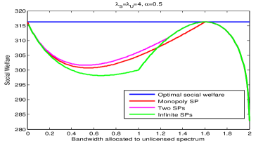
Figure 3: Social welfare versus unlicensed bandwidth with $\lambda_{S}=\lambda_{U}$.

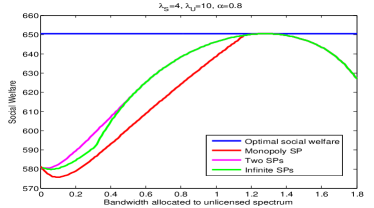
Figure 4: Social welfare versus $B_{U}$ with $\lambda_{S}<\lambda_{U}$. Here a monopolist can be efficient.

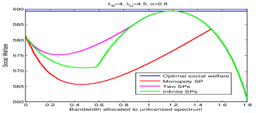
Figure 5: Social welfare versus $B_{U}$ with $\lambda_{S}<\lambda_{U}$. Here the monopolist is always inefficient.

VIII Conclusion

We have presented a model for allocating bandwidth in a HetNet with both licensed and unlicensed spectrum, taking into account the pricing strategies of the SPs. Our results characterize the equilibrium allocations assuming that the SPs maximize revenue or social welfare. For a monopoly SP that maximizes revenue, we show that the presence of a small amount of unlicensed spectrum may cause the SP to allocate more bandwidth to its competing small-cell network. However, when maximizing social welfare the SP always allocates less bandwidth with unlicensed spectrum. With multiple competing SPs the (unique) equilibrium is one of three different types, depending on the system parameters, including one in which the SPs do not allocate any bandwidth to a small-cell network (e.g., when the available bandwidth is small). We observe that in general, these equilibria do not achieve an efficient allocation corresponding to the maximum social welfare even when the number of competing SPs is large. In contrast, without unlicensed spectrum the equilibrium is always efficient for the class of $\alpha$-fair utility functions considered here.

We have used this framework to analyze the effect of unlicensed bandwidth on social welfare. If the small-cell network offers higher spectral efficiency than the unlicensed network, then according to our model, allocating all of the bandwidth as licensed is efficient. Otherwise, if the unlicensed network offers higher spectral efficiency, then we observe that there is a unique mix of unlicensed and licensed spectrum that maximizes social welfare, but that mix may or may not be efficient when the licensed spectrum is allocated to revenue-maximizing SPs.

In practice, a newly deployed licensed small-cell network may be based on LTE or WiFi, and the unlicensed (open access) network may be based on WiFi or LTE-U. Given the same density of access points, a managed LTE network would likely have the highest spectral efficiency, in which case, according to our model, allocating bands as licensed will maximize the social welfare. Of course, this assumes that the utility of a band depends only on the offered rate. Advocates of unlicensed spectrum have pointed to other properties, which are not taken into account here, such as lowering barriers to entry and the potential for developing new technologies and business models. Also not taken into account here is investment, which may pose different types of barriers to entry in licensed versus unlicensed spectrum. Incorporating investment within the framework presented here is left for future work.

Appendix A Proof of Theorem 1

We only discuss the case of $B_{S},B_{M}>0$. The sub-cases of either or both the variables being $0$ follow a similar logic with the obvious restriction of no users being served in the bands with no bandwidth.

1. We first show that the market always clears, i.e., all users would be served and the total rate supply is equal to the total rate demand.

Since the WiFi network on unlicensed spectrum is free to use, it’s obvious that all fixed users would be served. If there are some mobile users that are not served yet, the SP can increase the price in macro-cells so that users in macro-cells would request less rate, leading to the SP having some redundant rate to serve more mobile users. The SP can thus use up its rate in macro-cells at a higher price since the unserved mobile users would fill in, which then leads to larger revenue.

On the other hand, if all users are served but there is still some redundant rate available in macro-cells or small-cells, the SP can decrease the price in corresponding cells so that users now request a higher rate. Since $ru^{{}^{\prime}}(r)$, which is the revenue gained per user, increases with $r$, it’s easy to see the SP can gain more revenue by doing so.

As a result of the market clearing property we have the following important conclusion. In both the macro-cells and the small-cells, the per-user rate equals the allocated total rate (bandwidth times the spectral efficiency) divided by the mass of customers associated with macro-cells and the same-cells. The price for access is given precisely by the inverse of the demand function $D(\cdot)$ at this per-user rate.

2. We then prove the price choice and user association equilibrium in the two different scenarios, given the fixed bandwidth allocation.

Assume macro-cells only serve mobile users. This then implies that $R_{S}\geq R_{M}$ so that the boundary point would correspond to the point at which $R_{S}=R_{M}$ holds. It can be determined using the following steps.

$$K_{M}=N_{m}$$ (21)

$$u\Big{(}\frac{\lambda_{S}B_{S}R_{0}}{K_{S}}\Big{)}-\frac{\lambda_{S}B_{S}R_{0}}{K_{S}}u^{{}^{\prime}}\Big{(}\frac{\lambda_{S}B_{S}R_{0}}{K_{S}}\Big{)}=u\Big{(}\frac{C_{U}}{N_{f}-K_{S}}\Big{)}$$ (22)

$$R_{S}=\frac{\lambda_{S}B_{S}R_{0}}{K_{S}}=R_{M}=\frac{B_{M}R_{0}}{K_{M}}$$ (23)

The above equation simplify to

$$B_{S}=\frac{\kappa N_{f}B_{M}R_{0}-N_{m}C_{U}}{\kappa\lambda_{S}N_{m}R_{0}}=:B_{S}^{0}.$$ (24)

Therefore if $B_{S}$ is larger than $B_{S}^{0}$, it’s easy to see that the user equilibrium must be such that macro-cells only serve mobile users. In contrast, if $B_{S}$ is smaller than $B_{S}^{0}$, then $R_{S}<R_{M}$ holds assuming macro-cells only serve mobile users. As a result, some fixed users would have the incentive to associate with macro-cells and we would next prove that in this case at user equilibrium it’s indeed the case that some fixed users would associate with macro-cells.

Suppose $B_{S}<B_{S}^{0}$ and if macro-cells only serve mobile users such that the market clears, then we have $p_{M}<p_{S}$. The SP can then increases the price to $p_{M}^{{}^{\prime}}$, where $p_{M}<p_{M}^{{}^{\prime}}<p_{S}$, so that the mobile obtain a smaller rate creating some spare capacity. As a result, some fixed users in small-cells and WiFi network would switch to macro-cells, denote the total mass as $\delta$ and the mass of fixed users from small-cells switching being $\delta^{\prime}\leq\delta$. Note that before the price change $K_{M}=N_{m}$. The resulting revenue of the SP would then be :

$$S= B_{M}R_{0}u^{{}^{\prime}}\Big{(}R_{M}\frac{N_{m}}{N_{m}+\delta}\Big{)}$$

$$\qquad+\lambda_{S}B_{S}R_{0}u^{{}^{\prime}}\Big{(}R_{S}\frac{K_{S}}{K_{S}-\delta^{\prime}}\Big{)}$$

By Lemma 1 we can rewrite the revenue as:

$$S= B_{M}R_{0}u^{{}^{\prime}}\Big{(}R_{M}\frac{N_{m}}{N_{m}+\delta}\Big{)}$$

$$\qquad+\lambda_{S}B_{S}R_{0}u^{{}^{\prime}}\Big{(}R_{S}\frac{N_{f}}{N_{f}-\delta}\Big{)}$$

Then we have:

$$\frac{\partial S}{\partial\delta} =-{R_{M}^{{}^{\prime}}}^{2}u^{{}^{\prime\prime}}(R_{M}^{{}^{\prime}})+\frac{\lambda_{S}B_{S}R_{0}}{N_{f}-\delta}R_{S}^{{}^{\prime}}u^{{}^{\prime\prime}}(R_{S}^{{}^{\prime}})$$

$$=-{R_{M}^{{}^{\prime}}}^{2}u^{{}^{\prime\prime}}(R_{M}^{{}^{\prime}})+\frac{K_{S}}{N_{f}}\frac{\lambda_{S}B_{S}R_{0}}{K_{S}}\frac{N_{f}}{N_{f}-\delta}R_{S}^{{}^{\prime}}u^{{}^{\prime\prime}}(R_{S}^{{}^{\prime}})$$

$$>-{R_{M}^{{}^{\prime}}}^{2}u^{{}^{\prime\prime}}(R_{M}^{{}^{\prime}})+{R_{S}^{{}^{\prime}}}^{2}u^{{}^{\prime\prime}}(R_{S}^{{}^{\prime}}),$$

where $R_{S}^{\prime}=R_{S}\tfrac{K_{S}}{K_{S}-\delta^{\prime}}=R_{S}\tfrac{N_{f}}{N_{f}-\delta}$ and $R_{M}^{\prime}=R_{M}\tfrac{N_{m}}{N_{m}+\delta}$ are the new per user rates in the small-cells and macro-cells, respectively, after the shift of $\delta$ mass of fixed users to macro-cells.

Based on our assumptions, $r^{2}u^{{}^{\prime\prime}}(r)=-\alpha r^{1-\alpha}$ decreases with $r$, therefore as long as $R_{S}^{{}^{\prime}}<R_{M}^{{}^{\prime}}$, i.e., $p_{M}^{{}^{\prime}}<p_{S}^{{}^{\prime}}$, $S$ always increases with $\delta$. As a result, it’s always better for macro-cells to serve some fixed users in this case and the optimal price choice is $p_{M}=p_{S}$.

In mixed service scenario, we therefore have the following equations:

$$\begin{split}u\Big{(}\frac{C_{S}}{K_{S}}\Big{)}-p_{S}\frac{C_{S}}{K_{S}}&=u\Big{(}\frac{C_{U}}{K_{U}}\Big{)}=u\Big{(}\frac{C_{M}}{K_{M}}\Big{)}-p_{M}\frac{C_{M}}{K_{M}},\\ K_{U}+K_{S}+K_{M}&=N_{m}+N_{f},\\ D(p_{M})=R_{M}&=D(p_{S})=R_{S}=\frac{C_{S}+C_{M}}{K_{M}+K_{S}}.\end{split}$$ (25)

Using Lemma 1 we can get:

$$\begin{split}K_{U}&=(N_{f}+N_{m})\frac{C_{U}}{C_{U}+\kappa(C_{M}+C_{S})},\\ K_{M}&=(N_{f}+N_{m})\frac{\kappa C_{M}}{C_{U}+\kappa(C_{M}+C_{S})},\\ K_{S}&=(N_{f}+N_{m})\frac{\kappa C_{S}}{C_{U}+\kappa(C_{M}+C_{S})}.\end{split}$$ (26)

which gives the number of active users in terms of the network capacities.

Similarly, for the separate service scenario, writing the analogous conditions to (25) we can get:

$$\begin{split}K_{M}&=N_{m},\quad K_{S}=N_{f}\frac{\kappa C_{S}}{\kappa C_{S}+C_{U}},\\ K_{U}&=N_{f}\frac{C_{U}}{\kappa C_{S}+C_{U}}.\end{split}$$ (27)

Appendix B Proof of Theorem 2

1. We first prove that the optimal bandwidth allocation cannot occur at mixed service scenario. The revenue of the SP under the mixed service scenario is:

$$S= (B_{M}+\lambda_{S}B_{S})R_{0}u^{{}^{\prime}}\Big{(}\frac{(B_{M}+\lambda_{S}B_{S})R_{0}}{K_{M}+K_{S}}\Big{)}$$ (28)

$$= (B_{M}+\lambda_{S}B_{S})R_{0}u^{{}^{\prime}}\Big{(}\frac{C_{U}+\kappa(B_{M}+\lambda_{S}B_{S})R_{0}}{\kappa(N_{m}+N_{f})}\Big{)}$$ (29)

$$= (N_{m}+N_{f})Ru^{{}^{\prime}}(R)-\frac{C_{U}}{\kappa}u^{{}^{\prime}}(R)$$ (30)

where $R:=\frac{C_{U}+\kappa(B_{M}+\lambda_{S}B_{S})R_{0}}{\kappa(N_{m}+N_{f})}$ is the average rate in both macro-cells and small-cells.

Based on our assumptions, $Ru^{{}^{\prime}}(R)$ increases with $R$ and $u^{{}^{\prime}}(R)$ decreases with $R$, therefore it’s always beneficial to allocate more bandwidth to small-cells: since $\lambda_{S}>1$, $R$ increases with $B_{S}$. This means the optimal point cannot exist at a mixed service scenario.

2. We then prove the optimal bandwidth allocation scheme in separate service scenario. The revenue of the SP at separate service equilibrium is:

$$S= B_{M}R_{0}u^{{}^{\prime}}\Big{(}\frac{B_{M}R_{0}}{K_{M}}\Big{)}+\lambda_{S}B_{S}R_{0}u^{{}^{\prime}}\Big{(}\frac{\lambda_{S}B_{S}R_{0}}{K_{S}}\Big{)}$$ (31)

$$= N_{m}R_{M}u^{{}^{\prime}}(R_{M})+N_{f}R_{S}u^{{}^{\prime}}(R_{S})-\frac{C_{U}}{\kappa}u^{{}^{\prime}}(R_{S})$$ (32)

where $R_{M}=\frac{B_{M}R_{0}}{N_{m}},R_{S}=\frac{\lambda_{S}B_{S}R_{0}}{K_{S}}=\frac{\kappa\lambda_{S}B_{S}R_{0}+C_{U}}{\kappa N_{f}}$ are the average rate in macro-cells and small-cells, respectively.

It’s easy to verify for $\alpha$-fair utility functions, $R_{M}u^{{}^{\prime}}(R_{M}),R_{S}u^{{}^{\prime}}(R_{S})$ are concave increasing functions with respect to $B_{M}$ and $B_{S}$, respectively. Furthermore, $-u^{{}^{\prime}}(R_{S})$ is also a concave increasing function with respect to $B_{S}$. As a result, $S$ is a increasing with either $B_{S}$ or $B_{M}$. Therefore at optimal point the SP uses up all its total bandwidth and we have $B_{S}+B_{M}=1$. This further means $S$ is concave with $B_{S}$. As a result, the optimal point occurs at the point which uses up the total bandwidth and equalizes the marginal revenue increase with respect to per unit bandwidth increase in both macro-cells and small-cells, which can be achieved by straightforward calculation given below:

$$\begin{split}&\frac{1-\alpha}{\lambda_{S}}\big{(}\frac{B_{M}^{\text{rev}}R_{0}}{N_{m}}\big{)}^{-\alpha}=\Bigg{[}\big{(}\frac{\kappa\lambda_{S}B_{S}^{\text{rev}}R_{0}+C_{U}}{\kappa N_{f}}\big{)}^{-\alpha}\\ &\qquad\quad-\alpha\big{(}\frac{\kappa\lambda_{S}B_{S}^{\text{rev}}R_{0}+C_{U}}{\kappa N_{f}}\big{)}^{-\alpha}\frac{\kappa\lambda_{S}B_{S}^{\text{rev}}R_{0}}{\kappa\lambda_{S}B_{S}^{\text{rev}}R_{0}+C_{U}}\Bigg{]},\\ &\qquad B_{S}^{\text{rev}}+B_{M}^{\text{rev}}=B,\qquad B_{S}^{\text{rev}},B_{M}^{\text{rev}}\geq 0.\end{split}$$ (P1)

Appendix C Proof of Theorem 3

We first make the following definitions:

$$A_{1}= \Big{[}-\frac{\alpha\kappa\lambda_{S}B_{S}}{\kappa\lambda_{S}B_{S}+\lambda_{U}B_{U}}\bigg{(}\frac{\kappa\lambda_{S}B_{S}+\lambda_{U}B_{U}}{\kappa N_{f}}R_{0}\bigg{)}^{-\alpha}$$ (33)

$$\qquad+\bigg{(}\frac{\kappa\lambda_{S}B_{S}+\lambda_{U}B_{U}}{\kappa N_{f}}R_{0}\bigg{)}^{-\alpha}\Big{]}\lambda_{S}$$ (34)

$$A_{2}= (1-\alpha)\lambda_{S}\bigg{(}\frac{\lambda_{S}B_{S}R_{0}}{N_{f}}\bigg{)}^{-\alpha}$$ (35)

We only need to compare $A_{1}$ and $A_{2}$ at $\tilde{B}_{S}^{\text{rev}}$. By explicit calculation, this is given by:

$$A_{1}-A_{2}=\frac{M}{(\kappa\lambda_{S}\tilde{B}_{S}^{\text{rev}}R_{0}+C_{U})^{\alpha+1}(\lambda_{S}\tilde{B}_{S}^{\text{rev}}R_{0})^{\alpha}}$$ (36)

where $M=(1-\alpha)\big{[}(\kappa\lambda_{S}\tilde{B}_{S}^{\text{rev}}R_{0})^{\alpha+1}-(\kappa\lambda_{S}\tilde{B}_{S}^{\text{rev}}R_{0}+C_{U})^{\alpha+1}\big{]}-C_{U}(\kappa\lambda_{S}\tilde{B}_{S}^{\text{rev}}R_{0})^{\alpha}$.

It’s easy to verify that $M$ first increases with $C_{U}$ and then decreases with $C_{U}$. Moreover, $M=0$ when $C_{W}=0$. Therefore we only need to determine the other zero-crossing point $C_{U}^{th}$ by letting $M=0$. The conclusions in Theorem 3 then follow in a straightforward manner.

Appendix D Proof of Theorem 4

1. We first show that the market always clears, i.e., all users would be served and the total rate supply is equal to the total rate demand.

Since the WiFi network is free to use, again it’s obvious that all fixed users would be served. If there are some mobile users that are not served yet, the SP can increase the price in macro-cells so that users in macro-cells would request less rate and therefore it has some redundant rate to serve the mobile users. Since the function $K_{M}u(\frac{C_{M}}{K_{M}})$ increases with $K_{M}$, the social welfare is thus increased.

On the other hand, if all users are served but there is still some redundant rate available in macro-cells or small-cells. The SP can decrease the price in corresponding cells so that users now request higher rate, which naturally leads to higher social welfare.

2. We then prove the price choice and users association equilibrium in two different scenarios, depending on the fixed bandwidth allocation.

Similar to the analysis for revenue maximization, we first prove that at certain fixed bandwidth allocation, if macro-cells only serve mobile users and mobile users achieve larger rate than fixed users in small-cells, then the final user association should be that some fixed users associate with macro-cells and the price in macro-cells and small-cells should be the same.

Suppose macro-cells only serve mobile users and we have $p_{M}<p_{S},R_{M}>R_{S}$. The SP can increase the macro-cell price to $p_{M}^{{}^{\prime}}$, where $p_{M}<p_{M}^{{}^{\prime}}<p_{S}$. As a result, some fixed users in small-cells and WiFi network would switch to macro-cells, denote the mass of these fixed users as $\delta$ and $N_{t}=N_{m}+N_{f}=K_{M}+K_{S}+K_{U}$. By Lemma 1 we can show that the social welfare would then be :

$$\begin{split}\text{SW}=&(K_{M}+\delta)u\Big{(}R_{M}\frac{K_{M}}{K_{M}+\delta}\Big{)}\\ &\quad+K_{S}\frac{N_{t}-K_{M}-\delta}{N_{t}-K_{M}}u\Big{(}R_{S}\frac{N_{t}-K_{M}}{N_{t}-K_{M}-\delta}\Big{)}\\ &\quad+K_{U}\frac{N_{t}-K_{M}-\delta}{N_{t}-K_{M}}u\Big{(}R_{U}\frac{N_{t}-K_{M}}{N_{t}-K_{M}-\delta}\Big{)}.\end{split}$$ (37)

Then we have:

$$\frac{\partial\text{SW}}{\partial\delta}=u(R_{M}^{{}^{\prime}})-R_{M}^{{}^{\prime}}u^{{}^{\prime}}(R_{M}^{{}^{\prime}})-\frac{K_{S}}{N_{t}-K_{M}}\Big{[}u(R_{S}^{{}^{\prime}})-$$

$$\qquad R_{S}^{{}^{\prime}}u^{{}^{\prime}}(R_{S}^{{}^{\prime}})\Big{]}-\frac{K_{U}}{N_{t}-K_{M}}\Big{[}u(R_{U}^{{}^{\prime}})-R_{U}^{{}^{\prime}}u^{{}^{\prime}}(R_{U}^{{}^{\prime}})\Big{]}$$ (38)

For the $\alpha$-fair utility functions we use, it’s easy to verify that $u(r)-ru^{{}^{\prime}}(r)$ increases with $r$. We also have $R_{M}^{{}^{\prime}}>R_{S}^{{}^{\prime}}>R_{U}^{{}^{\prime}}$, thus

$$\frac{\partial\text{SW}}{\partial\delta} >u(R_{M}^{{}^{\prime}})-R_{M}^{{}^{\prime}}u^{{}^{\prime}}(R_{M}^{{}^{\prime}})-\big{[}u(R_{S}^{{}^{\prime}})-R_{S}^{{}^{\prime}}u^{{}^{\prime}}(R_{S}^{{}^{\prime}})\big{]}$$

$$>0.$$

Therefore the social welfare increases with $\delta$ in mixed service scenario as long as $p_{M}<p_{S}$. As a result, in this case some fixed users would associate with macro-cells, and the optimal price choice will be $p_{M}=p_{S}$.

3. Next, we show that the optimal bandwidth allocation is unique and only occurs at separate service scenario. The social welfare at mixed service scenario is:

$$\text{SW}=(K_{M}+K_{S})u(R)+K_{U}u(R_{U})$$ (39)

where $R=\frac{[\lambda_{U}B_{U}+\kappa(B_{M}+\lambda_{S}B_{S})]R_{0})}{\kappa(N_{m}+N_{f})}$, $R_{U}=\frac{[\lambda_{U}B_{U}+\kappa(B_{M}+\lambda_{S}B_{S})]R_{0})}{N_{m}+N_{f}}$ are the average user rate in licensed and unlicensed spectrum, respectively. Therefore we have:

$$\text{SW}= (K_{M}+K_{S})u(R)+K_{U}u(\kappa R)$$

$$= (N_{m}+N_{f})u(R)-K_{U}(u(R)-u(\kappa R))$$

$$= (N_{m}+N_{f})u(R)-C_{U}\frac{u(R)-u(\kappa R)}{\kappa R}$$ (40)

It’s easy to see that the first term is increasing with $R$. For $\alpha$-fair utility functions we use, it’s easy to verify the second term is decreasing with $R$. Therefore the social welfare increases with $R$, which leads to the conclusion that it’s always better to invest more bandwidth to small-cells. As a result, the optimal point cannot occur at mixed service scenario.

We then prove that the optimal bandwidth allocation is unique at separate service scenario.

$$\text{SW}=N_{m}u(R_{M})+K_{S}u(R_{S})+K_{U}u(R_{U})$$

$$R_{S}=\frac{\kappa\lambda_{S}B_{S}R_{0}+C_{U}}{\kappa N_{f}},R_{U}=\kappa R_{S}$$

$$K_{S}=\frac{\lambda_{S}B_{S}R_{0}}{R_{S}},K_{U}=\frac{C_{U}}{R_{U}}$$ (41)

We then have:

$$\text{SW}=N_{m}u(R_{M})+N_{f}u(R_{S})+\frac{C_{U}}{\kappa}[\frac{u(\kappa R_{S})-u(R_{S})}{R_{S}}]$$ (42)

Since $N_{m}u(R_{M})$ is concave increasing with $R_{M}$ and both $N_{f}u(R_{S})$, $\frac{u(\kappa R_{S})-u(R_{S})}{R_{S}}=-R_{S}^{-\alpha}$ are concave increasing with $R_{S}$. It’s easy to verify that social welfare is increasing with either $B_{S}$ or $B_{M}$ and therefore at optimal point we have $B_{S}+B_{M}=B$. By this we can further show that it is also a concave function with $B_{S}$ and therefore the optimal point is unique. At this optimal point, SP uses up the total bandwidth and equalizes the marginal social welfare increase of mobile users and fixed users with respect to per unit of bandwidth increase in macro-cells and small-cells. The optimal bandwidth allocation can be calculated as follows:

$$\left\{\begin{array}[]{ll}\frac{(N_{f})^{\alpha}\lambda_{S}\big{(}(\kappa^{\alpha}+\kappa)C_{U}+\kappa^{\alpha+1}\lambda_{S}B_{S}^{\text{sw}}R_{0}\big{)}}{(\kappa\lambda_{S}B_{S}^{\text{sw}}R_{0}+C_{U})^{\alpha+1}}=(\frac{B_{M}^{\text{sw}}R_{0}}{N_{m}})^{-\alpha},\\ B_{S}^{\text{sw}}+B_{M}^{\text{sw}}=1,\qquad B_{S}^{\text{sw}},B_{M}^{\text{sw}}\geq 0.\end{array}\right.$$

4. Last, we prove $B_{S}^{\text{sw}}<\tilde{B}_{S}^{\text{sw}}$. We first define some notations.

$$A_{3}=\frac{(N_{f})^{\alpha}\lambda_{S}\big{[}(\kappa^{\alpha}+\kappa)C_{U}+\kappa^{\alpha+1}\lambda_{S}\tilde{B}_{S}^{*}R_{0}\big{]}}{(\kappa\lambda_{S}\tilde{B}_{S}^{*}R_{0}+C_{U})^{\alpha+1}}$$

$$A_{4}=\lambda_{S}\big{(}\frac{\lambda_{S}\tilde{B}_{S}^{**}R_{0}}{N_{f}}\big{)}^{-\alpha}$$ (42)

We only need to compare $A_{3}$ and $A_{4}$ at $\tilde{B}_{S}^{\text{sw}}$. It turns out that:

$$\frac{A_{3}-A_{4}}{\lambda_{S}R_{0}(N_{f})^{\alpha}}=\frac{M}{(\lambda_{S}\tilde{B}_{S}^{\text{sw}}R_{0})^{\alpha}(\kappa\lambda_{S}\tilde{B}_{S}^{\text{sw}}R_{0}+C_{U})^{\alpha+1}}$$

$$M=(\kappa^{\alpha}+\kappa)C_{U}(\lambda_{S}\tilde{B}_{S}^{\text{sw}}R_{0})^{\alpha}+\kappa^{\alpha+1}(\lambda_{S}\tilde{B}_{S}^{\text{sw}}R_{0})^{\alpha+1}$$

$$-(\kappa\lambda_{S}\tilde{B}_{S}^{\text{sw}}R_{0}+C_{U})^{\alpha+1}$$ (43)

We then have:

$$\frac{\partial M}{\partial C_{U}}= (\alpha+1)\Big{[}(\kappa\lambda_{S}\tilde{B}_{S}^{\text{sw}}R_{0})^{\alpha}-(\kappa\lambda_{S}\tilde{B}_{S}^{\text{sw}}R_{0}+C_{U})^{\alpha}\Big{]}$$

$$< 0,\quad\forall C_{U}>0.$$ (44)

Since when $C_{U}=0$, $A_{3}=A_{4}$. Therefore $A_{3}<A_{4}$ when $C_{U}>0$. As a result, compared with the scenario without unlicensed spectrum, the SP should always invest less bandwidth to small-cells in terms of social welfare maximization.

Appendix E Proof of Theorem 5

The proof is essentially the same as the proof for the price choice and user association equilibrium for monopoly service provider scenario. The only difference is that we need to prove the prices must be equal across all small-cells or macro-cells with multiple SPs.

Suppose one SP $i$ has lower small-cell price $p_{i,S}$ than the other SP $j$. SP $i$ can increase the price to $p_{i,S}^{{}^{\prime}}$ satisfying $p_{i,S}<p_{i,S}^{{}^{\prime}}<p_{j,S}$. As a result, SP $i$ would attract some users which used to associate with SP $j$’s small-cell or some users from unlicensed access and still use up all the rate with a higher price. Therefore SP $i$ can increase its revenue by doing so. Thus, at price equilibrium all small-cell price must be equal. The proof for all macro-cell prices must be equal is done similarly.

Appendix F Proof of Theorem 6

We prove the theorem in the following steps.

1. First, we prove that no Nash equilibrium exists at mixed service scenario. It’s easy to see the revenue of SP $i$ in this case is:

$$S_{i}=(B_{i,M}+\lambda_{S}B_{i,S})R_{0}u^{{}^{\prime}}\Big{[}\frac{\sum\limits_{j=1}^{N}(B_{j,M}+\lambda_{S}B_{j,S})R_{0}}{K_{M}+K_{S}}\Big{]}$$ (45)

$$=(K_{M}+K_{S})Ru^{{}^{\prime}}(R)-\sum\limits_{j\neq i}^{N}(B_{j,M}+\lambda_{S}B_{j,S})R_{0}u^{{}^{\prime}}(R)$$ (46)

$$K_{M}+K_{S}=N_{m}+N_{f}-\frac{(N_{m}+N_{f})C_{U}}{C_{U}+\kappa\sum\limits_{j=1}^{N}(B_{j,M}+\lambda_{S}B_{j,S})R_{0}}$$ (47)

$$R=\frac{C_{U}+\kappa\sum\limits_{j=1}^{N}(B_{j,M}+\lambda_{S}B_{j,S})R_{0}}{\kappa(N_{m}+N_{f})}$$ (48)

It’s easy to see that $R$ and $K_{M}+K_{S}$ both increase with $B_{i,S}$. Meanwhile, $Ru^{{}^{\prime}}(R)$ increases with $R$ and $u^{{}^{\prime}}(R)$ decreases with $R$. As a result, $S_{i}$ increases with $B_{i,S}$ and every SP would have incentive to invest more bandwidth to small-cells, which would finally push the equilibrium to separate service scenario. Therefore no Nash equilibrium exists in mixed service scenario.

2. We next prove that there always exists a Nash equilibrium at separate service scenario. The revenue of SP $i$ in this case is:

$$S_{i}= S_{i,M}+S_{i,S}$$

$$= B_{i,M}R_{0}u^{{}^{\prime}}(R_{M})+\lambda_{S}B_{i,S}R_{0}u^{{}^{\prime}}(R_{S})$$

$$= B_{i,M}R_{0}u^{{}^{\prime}}\Big{(}\frac{\sum\limits_{j=1}^{N}B_{j,M}R_{0}}{N_{m}}\Big{)}+\lambda_{S}B_{i,S}R_{0}u^{{}^{\prime}}\Big{(}\frac{\sum\limits_{j=1}^{N}\lambda_{S}B_{j,S}R_{0}}{K_{S}}\Big{)}$$ (49)

It’s easy to verify:

$$\frac{\partial S_{i,M}}{\partial B_{i,M}}= R_{0}\big{[}u^{{}^{\prime}}(R_{M})+\frac{B_{i,M}R_{0}}{N_{m}}u^{{}^{\prime\prime}}(R_{M})\big{]}$$

$$= R_{0}\big{[}u^{{}^{\prime}}(R_{M})+R_{M}u^{{}^{\prime\prime}}(R_{M})-\frac{\sum\limits_{j\neq i}B_{j,M}R_{0}}{N_{m}}u^{{}^{\prime\prime}}(R_{M})\big{]}$$

$$> 0$$ (50)

$$\frac{\partial S_{i,S}}{\partial B_{i,S}}= \lambda_{S}R_{0}\big{[}u^{{}^{\prime}}(R_{S})+\frac{\lambda_{S}B_{i,S}R_{0}}{N_{f}}u^{{}^{\prime\prime}}(R_{S})\big{]}$$

$$= \lambda_{S}R_{0}\big{[}u^{{}^{\prime}}(R_{S})+\frac{\sum\limits_{j=1}^{N}\lambda_{S}B_{j,S}R_{0}}{N_{f}}u^{{}^{\prime\prime}}(R_{S})$$

$$-\frac{\sum\limits_{j\neq i}\lambda_{S}B_{j,S}R_{0}}{N_{f}}u^{{}^{\prime\prime}}(R_{S})\big{]}$$

$$= \lambda_{S}R_{0}\big{[}u^{{}^{\prime}}(R_{S})+R_{S}u^{{}^{\prime\prime}}(R_{S})$$

$$-\frac{\lambda_{S}C_{U}}{\kappa N_{f}}u^{{}^{\prime\prime}}(R_{S})-\frac{\sum\limits_{j\neq i}\lambda_{S}B_{j,S}R_{0}}{N_{f}}u^{{}^{\prime\prime}}(R_{S})\big{]}>0$$ (51)

Since $u^{{}^{\prime}}(r)+ru^{{}^{\prime\prime}}(r)$ decreases with $r$ and $u^{{}^{\prime\prime}}(r)$ increases with $r$, it’s easy to verify $S_{i,M}$ and $S_{i,S}$ are both concave increasing with $B_{i,M}$ and $B_{i,S}$ respectively. This also indicates all SPs would always use up their total bandwidth, i.e., $B_{i,S}+B_{i,M}=B_{I}$. By this we can further show $S_{i}$ is a concave function with $B_{i,S}$. Moreover, the constraint on separate service scenario are linear with $B_{i,S}$. We can then apply Rosen’s theorem on concave games [20] to prove the existence of Nash equilibrium.

3. For the third step, we prove that fixed users in small-cells achieve higher average rate than mobile users in macro-cells. This is equivalent to say $R_{S}>R_{M}$ at equilibrium.

We only need to rule out the possibility that $R_{S}=R_{M}$ since we already showed that the Nash equilibrium falls into separate service scenario. Denote the group of SPs that only allocate bandwidth to small-cells (macro-cells) as $G_{S}(G_{M})$ and the group of SPs that allocate bandwidth to both cells as $G_{MS}$, then we have:

$$\forall i\in G_{S},B_{i,S}=B_{i},B_{i,M}=0$$

$$\forall j\in G_{M}\cup G_{MS},\frac{\partial S_{j}}{B_{j,S}}\leq 0$$ (52)

If $R_{S}=R_{M}=R$ holds, then $\forall j\in G_{M}\cup G_{MS}$, we have:

$$\frac{\partial S_{j}}{\partial B_{j,S}}= \lambda_{S}R_{0}\Big{[}u^{{}^{\prime}}(R_{S})+\frac{\lambda_{S}B_{j,S}R_{0}}{N_{f}}u^{{}^{\prime\prime}}(R_{S})\Big{]}$$

$$-R_{0}\Big{[}u^{{}^{\prime}}(R_{M})+\frac{B_{j,M}R_{0}}{N_{m}}u{{}^{\prime\prime}}(R_{M})\Big{]}$$

$$= (\lambda_{S}-1)u^{{}^{\prime}}(R)+\Big{[}\frac{\lambda_{S}B_{j,S}R_{0}}{N_{f}}-\frac{B_{j,M}R_{0}}{N_{m}}\Big{]}u^{{}^{\prime\prime}}(R)$$

$$\leq 0$$ (53)

Therefore $\forall j\in G_{M}\cup G_{MS}$, we have:

$$\frac{\lambda_{S}B_{j,S}R_{0}}{N_{f}}\geq\frac{B_{j,M}R_{0}}{N_{m}}$$ (54)

As a result, the following holds:

$$R_{S}= \sum\limits_{j\in G_{M}\cup G_{MS}}\frac{\lambda_{S}B_{j,S}R_{0}}{N_{f}}+\sum\limits_{i\in G_{S}}\frac{\lambda_{S}B_{i}R_{0}}{N_{f}}>$$ (55)

$$\sum\limits_{j\in G_{M}\cup G_{MS}}\frac{B_{j,M}R_{0}}{N_{m}}=R_{M}$$ (56)

Therefore we have a contradiction.

4. We then show that at Nash equilibrium it is impossible that one SP only allocates bandwidth to macro-cells while the other SP only allocates bandwidth to small-cells.

Suppose SP $i$ only allocates bandwidth to macro-cells while SP $j$ only allocates bandwidth to small-cells. Then we have:

$$\frac{\partial S_{i}}{\partial B_{i,S}}= \lambda_{S}R_{0}u^{{}^{\prime}}(R_{S})-R_{0}\Big{[}u^{{}^{\prime}}(R_{M})+\frac{B_{i,M}R_{0}}{N_{m}}u{{}^{\prime\prime}}(R_{M})\Big{]}$$

$$\leq 0$$ (57)

$$\frac{\partial S_{j}}{\partial B_{j,S}}= \lambda_{S}R_{0}\Big{[}u^{{}^{\prime}}(R_{S})+\frac{\lambda_{S}B_{j,S}R_{0}}{N_{f}}u^{{}^{\prime\prime}}(R_{S})\Big{]}-R_{0}u^{{}^{\prime}}(R_{M})$$

$$\geq 0$$ (58)

which would yield:

$$-\frac{B_{i,M}R_{0}}{N_{m}}u{{}^{\prime\prime}}(R_{M})\leq\lambda_{S}\frac{\lambda_{S}B_{j,S}R_{0}}{N_{f}}u^{{}^{\prime\prime}}(R_{S})$$ (59)

Clearly we have a contradiction then.

5. After step 4, it’s clear that there are only five possible Nash equilibrium types:

• Small-only Nash equilibrium(SNE): All SPs only allocate bandwidth to small-cells.

• Macro-only Nash equilibrium(MNE): All SPs only allocate bandwidth to macro-cells.

• Macro-Small Nash Equilibrium (MSNE): All SPs allocate bandwidth to both macro- and small-cells.

• Macro-Preferred Nash Equilibrium (MPNE): Some SPs allocate bandwidth to both small– and macro-cells while the other SPs only allocate bandwidth to macro-cells.

• Small-Preferred Nash Equilibrium (SPNE): Some SPs allocate bandwidth to both small– and macro-cells while the other SPs only allocate bandwidth to small-cells.

We next prove that SNE cannot exist.

The marginal revenue increase with respect to per unit bandwidth increase in macro-cells for SP $i$ is given by:

$$\frac{\partial S_{i}}{\partial B_{i,M}}=R_{0}\Big{[}u^{{}^{\prime}}(R_{M})+\frac{B_{i,M}R_{0}}{N_{m}}u^{{}^{\prime\prime}}(R_{M})\Big{]}$$ (60)

It can be easily shown that for $\alpha$-fair utility functions, the marginal revenue increase with respect to per unit bandwidth increase in macro-cells goes to infinity when $B_{M}$ is near 0. As a result, SNE cannot exist.

However, the above argument doesn’t apply to MNE. At first glance, it seems that when all SPs only allocate bandwidth to macro-cells, the marginal revenue increase with respect to per unit bandwidth in small-cells also goes to infinity when $B_{S}$ is near 0. Actually, the marginal revenue increase does go to infinity when $R_{S}$ is near 0. However, $R_{S}$ doesn’t go to 0 when $B_{S}$ goes to 0. In fact, $R_{S}$ is discontinuous at the point 0. We have the following:

$$R_{S}=\frac{\kappa\lambda_{S}B_{S}R_{0}+C_{U}}{\kappa N_{f}}, B_{S}>0;$$ (61)

$$R_{S}=0, B_{S}=0.$$ (62)

Therefore as $B_{S}\rightarrow 0^{+},R_{S}\rightarrow\frac{C_{U}}{\kappa N_{f}}>0$.

6. The fact that SPNE cannot exist requires more work and in this part we would focus on it. At SPNE, we know that there exist SPs $i,j$ such that:

$$\frac{\partial S_{i}}{\partial B_{i,S}}\geq 0,B_{i,S}=B_{i},B_{i,M}=0$$ (63)

$$\frac{\partial S_{j}}{\partial B_{j,S}}=0,B_{j,S}>0,B_{j,M}>0$$ (64)

We therefore have:

$$\lambda_{F}\Big{[}u^{{}^{\prime}}(R_{S})+\frac{\lambda_{S}B_{i,S}R_{0}}{N_{f}}u{{}^{\prime\prime}}(R_{S})\Big{]}\geq u^{{}^{\prime}}(R_{M})$$ (65)

$$\lambda_{S}\Big{[}u^{{}^{\prime}}(R_{S})+\frac{\lambda_{S}B_{i,S}R_{0}}{N_{f}}u{{}^{\prime\prime}}(R_{S})\Big{]}=u^{{}^{\prime}}(R_{M})+$$

$$\frac{B_{i,M}R_{0}}{N_{m}}u^{{}^{\prime\prime}}(R_{M})$$ (66)

From the first inequality above, we can easily conclude that:

$$\lambda_{S}u^{{}^{\prime}}(R_{S})>u^{{}^{\prime}}(R_{M})$$ (67)

Next, we consider the group of service providers that allocate bandwidth to both cells, denoted as $G_{MS}$ and assume $|G_{MS}|=L$.

$$\forall j\in G_{MS},\frac{\partial S_{j}}{\partial B_{j,S}}=0,B_{j,S}>0,B_{j,M}>0$$ (68)

We then have:

$$\lambda_{S}\Big{[}Lu^{{}^{\prime}}(R_{S})+\frac{\lambda_{S}\sum\limits_{j\in G_{MS}}B_{j,S}R_{0}}{N_{f}}u{{}^{\prime\prime}}(R_{S})\Big{]}=$$

$$Lu^{{}^{\prime}}(R_{M})+\frac{\sum\limits_{j\in G_{MS}}B_{j,M}R_{0}}{N_{m}}u^{{}^{\prime\prime}}(R_{M})$$ (69)

It’s easy to get:

$$\lambda_{S}\Big{[}Lu^{{}^{\prime}}(R_{S})+\frac{\lambda_{S}\sum\limits_{j\in\mathcal{N}}B_{j,S}R_{0}}{N_{f}}u{{}^{\prime\prime}}(R_{S})\Big{]}<$$

$$Lu^{{}^{\prime}}(R_{M})+R_{M}u^{{}^{\prime\prime}}(R_{M})$$ (70)

Together with inequality 67, we can get the second inequality:

$$\lambda_{S}\Big{[}u^{{}^{\prime}}(R_{S})+\frac{\lambda_{S}\sum\limits_{j\in\mathcal{N}}B_{j,S}R_{0}}{N_{f}}u{{}^{\prime\prime}}(R_{S})\Big{]}<$$

$$u^{{}^{\prime}}(R_{M})+R_{M}u^{{}^{\prime\prime}}(R_{M})$$ (71)

For $\alpha$-fair utility functions, we have:

$$u^{{}^{\prime}}(R_{M})+R_{M}u^{{}^{\prime\prime}}(R_{M})=(1-\alpha)u^{{}^{\prime}}(R_{M})$$ (72)

However, we also have:

$$\lambda_{S}\Big{[}u^{{}^{\prime}}(R_{S})+\frac{\lambda_{S}\sum\limits_{j\in\mathcal{N}}B_{j,S}R_{0}}{N_{f}}u{{}^{\prime\prime}}(R_{S})\Big{]}-(1-\alpha)\lambda_{S}u^{{}^{\prime}}(R_{S})$$

$$=\lambda_{S}\Big{[}\alpha u^{{}^{\prime}}(R_{S})+\frac{\lambda_{S}\sum\limits_{j\in\mathcal{N}}B_{j,S}R_{0}}{N_{f}}u{{}^{\prime\prime}}(R_{S})\Big{]}$$

$$>\lambda_{S}\Big{[}\alpha u^{{}^{\prime}}(R_{S})+R_{S}u{{}^{\prime\prime}}(R_{S})\Big{]}$$

$$=\lambda_{S}\alpha R_{S}^{-\alpha}-\lambda_{S}\alpha R_{S}^{-\alpha}=0$$ (73)

Therefore the two inequalities have a contradiction. As a result, SPNE cannot exist.

7. We next prove that MSNE, MNE and MPNE cannot coexist. First it’s easy to verify that at MSNE, MNE and MPNE, we have the following:

$$\text{MSNE}:\quad \lambda_{S}\Big{[}Nu^{{}^{\prime}}(R_{S})+\frac{\lambda_{S}\sum\limits_{i\in\mathcal{N}}B_{i,S}R_{0}}{N_{f}}u^{{}^{\prime\prime}}(R_{S})\Big{]}$$

$$=Nu^{{}^{\prime}}(R_{M})+R_{M}u^{{}^{\prime\prime}}(R_{M})$$ (74)

$$\text{MNE or MPNE}:\quad \lambda_{S}\Big{[}Nu^{{}^{\prime}}(R_{S})+\frac{\lambda_{S}\sum\limits_{i\in\mathcal{N}}B_{i,S}R_{0}}{N_{f}}u^{{}^{\prime\prime}}(R_{S})\Big{]}$$

$$\leq Nu^{{}^{\prime}}(R_{M})+R_{M}u^{{}^{\prime\prime}}(R_{M})$$ (75)

We can show that the LHS is a decreasing function with $R_{S}$, since we have:

$$R_{S}=\frac{C_{U}+\kappa\lambda_{S}\sum\limits_{i\in\mathcal{N}}B_{i,S}R_{0}}{\kappa N_{f}}$$ (76)

Therefore we have:

$$\text{LHS}= \lambda_{S}\big{[}u^{{}^{\prime}}(R_{S})+R_{S}u^{{}^{\prime\prime}}(R_{S})\big{]}+(N-1)\lambda_{S}u^{{}^{\prime}}(R_{S})$$ (77)

$$-\frac{\lambda_{S}C_{U}}{\kappa N_{f}}u^{{}^{\prime\prime}}(R_{S})$$ (78)

which is decreasing with $R_{S}$.

Similarly, RHS is also a decreasing function with $R_{M}$.

Now suppose for the same set of parameters, we have one MNE or MPNE and another MSNE, denote the corresponding bandwidth allocation profile as $\mathbf{B}$ and $\bar{\mathbf{B}}$, respectively. Then we must have:

$$\bar{R_{S}}\leq R_{S},\bar{R_{M}}\geq R_{M}$$ (79)

Now it is clearly shown that MNE and MSNE cannot coexist since for MNE we have $R_{M}>\bar{R_{M}}$.

If $\mathbf{B}$ corresponds to MPNE, we can conclude that at MSNE, some SPs must have less bandwidth allocation to small-cells than that of MPNE. Denote this group of SPs as $G_{S-}$ and assume $|G_{MS-}|=L$, we have:

$$\forall j\in G_{S-},\frac{\partial S_{j}}{\partial B_{j,S}}=0,\frac{\partial\bar{S_{j}}}{\partial\bar{B}_{j,S}}\leq 0$$ (80)

Summing up, we get:

$$\lambda_{S}\Big{[}Lu^{{}^{\prime}}(R_{S})+\frac{\lambda_{S}\sum\limits_{j\in G_{S-}}B_{j,S}R_{0}}{N_{f}}u^{{}^{\prime\prime}}(R_{S})\Big{]}=$$

$$Lu^{{}^{\prime}}(R_{M})+\frac{\sum\limits_{j\in G_{S-}}B_{j,M}R_{0}}{N_{m}}u^{{}^{\prime\prime}}(R_{M})$$ (81)

$$\lambda_{S}\Big{[}Lu^{{}^{\prime}}(\bar{R_{S}})+\frac{\lambda_{S}\sum\limits_{j\in G_{S-}}\bar{B_{j,S}}R_{0}}{N_{f}}u^{{}^{\prime\prime}}(\bar{R_{S}})\Big{]}\leq$$

$$Lu^{{}^{\prime}}(\bar{R_{M}})+\frac{\sum\limits_{j\in G_{S-}}\bar{B_{j,M}}R_{0}}{N_{m}}u^{{}^{\prime\prime}}(\bar{R_{M}})$$ (82)

Rearranging some of the terms, we have:

$$\lambda_{S}\Big{[}Lu^{{}^{\prime}}(R_{S})+\frac{\lambda_{S}\sum\limits_{j\in\mathcal{N}}B_{j,S}R_{0}}{N_{f}}u^{{}^{\prime\prime}}(R_{S})\Big{]}=$$

$$Lu^{{}^{\prime}}(R_{M})+R_{M}u^{{}^{\prime\prime}}(R_{M})+\lambda_{S}\frac{\lambda_{S}\sum\limits_{j\notin{G_{S-}}}B_{j,S}R_{0}}{N_{f}}u^{{}^{\prime\prime}}(R_{S})$$

$$-\frac{\sum\limits_{j\notin G_{S-}}B_{j,M}R_{0}}{N_{m}}u^{{}^{\prime\prime}}(R_{M})$$ (83)

$$\lambda_{S}\Big{[}Lu^{{}^{\prime}}(\bar{R_{S}})+\frac{\lambda_{S}\sum\limits_{j\in\mathcal{N}}\bar{B_{j,S}}R_{0}}{N_{f}}u^{{}^{\prime\prime}}(\bar{R_{S}})\Big{]}\leq$$

$$Lu^{{}^{\prime}}(\bar{R_{M}})+\bar{R_{M}}u^{{}^{\prime\prime}}(\bar{R_{M}})+\lambda_{S}\frac{\lambda_{S}\sum\limits_{j\notin{G_{S-}}}\bar{B_{j,S}}R_{0}}{N_{f}}u^{{}^{\prime\prime}}(\bar{R_{S}})$$

$$-\frac{\sum\limits_{j\notin G_{S-}}\bar{B_{j,M}}R_{0}}{N_{m}}u^{{}^{\prime\prime}}(\bar{R_{M}})$$ (84)

However, we also have:

$$\forall j\not\in G_{S-},\bar{B_{j,S}}\geq B_{j,S},\bar{B_{j,M}}\leq B_{j,M}$$ (85)

We already showed that LHS decreases with $R_{S}$ and the first two terms on RHS decreases with $R_{M}$. For $\alpha$-fair utility functions, $u^{{}^{\prime\prime}}(r)<0$ increases with $r$. Combining with the fact that $\bar{R_{S}}\leq R_{S},\bar{R_{M}}\geq R_{M}$ and noticing that at least one of the inequalities must be strict inequality, we can also conclude:

$$\lambda_{S}\Big{[}Lu^{{}^{\prime}}(\bar{R_{S}})+\frac{\lambda_{S}\sum\limits_{j\in\mathcal{N}}\bar{B_{j,S}}R_{0}}{N_{f}}u^{{}^{\prime\prime}}(\bar{R_{S}})\Big{]}>$$

$$Lu^{{}^{\prime}}(\bar{R_{M}})+\bar{R_{M}}u^{{}^{\prime\prime}}(\bar{R_{M}})+\lambda_{S}\frac{\lambda_{S}\sum\limits_{j\notin{G_{S-}}}\bar{B_{j,S}}R_{0}}{N_{f}}u^{{}^{\prime\prime}}(\bar{R_{S}})$$

$$-\frac{\sum\limits_{j\notin G_{S-}}\bar{B_{j,M}}R_{0}}{N_{m}}u^{{}^{\prime\prime}}(\bar{R_{M}})$$ (86)

Clearly we have a contradiction then. As a result, MSNE and MPNE cannot coexist.

We then only need to show MNE and MPNE cannot coexist. It can be proved in a similar way as we proved MSNE and MPNE cannot coexist introduced above. We now focus on the group of SPs which decrease bandwidth allocation to small-cells and apply the same procedures to get a contradiction.

8. Finally, we need to show that within MSNE, MNE or MPNE, the Nash equilibrium is unique.

The uniqueness of MNE is trivial.

The uniqueness of MPNE can be proved in a similar way in which we proved MSNE and MPNE cannot coexist. Here we don’t repeat the steps.

The uniqueness of MSNE can also be proved similarly. However, here we use another method. It’s easy to see that at MSNE, we have the following system of equations.

$$\left\{\begin{array}[]{ll}\lambda_{S}[Nu^{{}^{\prime}}(R_{S})+\frac{\lambda_{S}\sum\limits_{i\in\mathcal{N}}B_{i,S}R_{0}}{N_{f}}u^{{}^{\prime\prime}}(R_{S})]\\ =Nu^{{}^{\prime}}(R_{M})+R_{M}u^{{}^{\prime\prime}}(R_{M})\\ \frac{\lambda_{S}^{2}\Delta B_{ij,S}}{N_{f}}u^{{}^{\prime\prime}}(R_{S})=\frac{\Delta B_{ij,M}}{N_{m}}u^{{}^{\prime\prime}}(R_{M})\end{array}\right.$$

where $\Delta B_{ij,S}=B_{i,S}-B_{j,S}$ is the difference of bandwidth allocation to small-cells between SP $i$ and SP $j$, the same for $\Delta B_{ij,M}$.

By the monotonicity of both LHS and RHS with respect to $R_{S}$ and $R_{M}$, the first equation we can uniquely determine $\sum\limits_{i=1}^{N}B_{i,S}$. While the second equation characterizes the relationship of $B_{i,S}$ between any pair of service providers, as a result the above equation system is essentially a linear equation system with $N$ unknowns and $N$ independent linear equations. Thus if there is a solution to the equation system, it must be unique.

Appendix G MSNE Conditions and Properties

The bandwidth allocation at an MSNE can be computed via the following system of equations:

$$\left\{\begin{array}[]{ll}\lambda_{S}[Nu^{{}^{\prime}}(R_{S})+\frac{\lambda_{S}\sum\limits_{i\in\mathcal{N}}B_{i,S}R_{0}}{N_{f}}u^{{}^{\prime\prime}}(R_{S})]\\ =Nu^{{}^{\prime}}(R_{M})+R_{M}u^{{}^{\prime\prime}}(R_{M})\\ \frac{\lambda_{S}^{2}\Delta B_{ij,S}}{N_{f}}u^{{}^{\prime\prime}}(R_{S})=\frac{\Delta B_{ij,M}}{N_{m}}u^{{}^{\prime\prime}}(R_{M})\end{array}\right.$$

where $\Delta B_{ij,S}=B_{i,S}-B_{j,S}$ is the difference of bandwidth allocation to small-cells between SP $i$ and SP $j$, the same for $\Delta B_{ij,M}$.

Proposition 3 results in the following corollary in the symmetric setting where all SPs have the same bandwidths, i.e., $B_{i}\equiv B$ for all $i\in\mathcal{N}$.

Corollary 1

If all SPs have the same bandwidths $B$ and

$$C_{U}\geq R_{0}NB\left(\frac{\lambda_{S}}{1-\frac{\alpha}{N}}\right)^{\frac{1}{\alpha}}\frac{\kappa N_{f}}{N_{m}},$$ (87)

then we have an MNE with

$$\begin{split}&K_{M}=N_{m},K_{S}=0,K_{U}=N_{f},\\ &R_{M}=\frac{NBR_{0}}{N_{m}},R_{S}=0,R_{U}=\frac{C_{U}}{N_{f}}.\end{split}$$ (88)

Otherwise we have an MSNE in which all SPs have the same bandwidth allocation and can be determined by solving the following equations

$$\begin{split}&\bigg{(}1-\frac{\alpha}{N}\bigg{)}\left(\frac{N_{m}}{NB_{M}R_{0}}\right)^{\alpha}=\left(\frac{\kappa N_{f}}{\kappa NB_{S}\lambda_{S}R_{0}+C_{U}}\right)^{\alpha}\\ &\qquad\qquad\qquad\qquad\times\lambda_{S}\left(1-\alpha\frac{\kappa\lambda_{S}B_{S}R_{0}}{\kappa NB_{S}\lambda_{S}R_{0}+C_{U}}\right)\\ &B_{S}+B_{M}=B,\qquad B_{S},B_{M}>0.\end{split}$$ (89)

Using Corollary 1 we can analyze the asymptotic scenario of $N\rightarrow\infty$ as given below.

Proposition 5

Assume that the total amount of bandwidth of $N$ SPs is fixed to be $B$ and each SP $i$ gets the same proportion $B_{i}=\frac{B}{N}$. If we have

$$B_{U}\lambda_{U}>B\frac{\kappa N_{f}\lambda_{S}^{\frac{1}{\alpha}}}{N_{m}},$$ (90)

then there exists an $N^{*}(B_{U}\lambda_{U})$ such that for all $N>N^{*}(B_{U}\lambda_{U})$ we have an MNE so that $B_{i,M}=B/N$ and $B_{i,S}=0$ for all $i\in\mathcal{N}$. Otherwise we always have an MSNE, with $\lim_{N\rightarrow\infty}(NB_{i,M},NB_{i,S})=(B_{M},B_{S})$ for all $i$ with

$$B_{S}=\frac{B-\frac{B_{U}\lambda_{U}N_{m}}{\kappa N_{f}\lambda_{S}^{\frac{1}{\alpha}}}}{1+\frac{\lambda_{S}N_{m}}{\lambda_{S}^{\frac{1}{\alpha}}N_{f}}},B_{M}=\frac{\bigg{(}B+B_{U}\frac{\lambda_{U}}{\kappa\lambda_{S}}\bigg{)}\frac{\lambda_{S}N_{m}}{\lambda_{S}^{\frac{1}{\alpha}}N_{f}}}{1+\frac{\lambda_{S}N_{m}}{\lambda_{S}^{\frac{1}{\alpha}}N_{f}}}.$$ (91)

Furthermore,

$$\begin{split}&K_{S}=\frac{\kappa B_{S}\lambda_{S}N_{f}}{\kappa B_{S}\lambda_{S}+B_{U}\lambda_{U}},K_{U}=\frac{B_{U}\lambda_{U}N_{f}}{\kappa B_{S}\lambda_{S}+B_{U}\lambda_{U}},\\ &K_{M}=N_{m},R_{S}=\frac{R_{0}(\kappa B_{S}\lambda_{S}+B_{U}\lambda_{U})}{\kappa N_{f}},\\ &R_{M}=\frac{B_{M}R_{0}}{N_{m}},R_{U}=\frac{R_{0}(\kappa B_{S}\lambda_{S}+B_{U}\lambda_{U})}{N_{f}}.\end{split}$$ (92)

Appendix H Proof of Proposition 2

The equilibrium equations for MSNE in scenarios with and without unlicensed spectrum are given below:

$$\text{With}:\lambda_{S}\Big{[}Nu^{{}^{\prime}}(R_{S})+\frac{\lambda_{S}B_{S}R_{0}}{N_{f}}u^{{}^{\prime\prime}}(R_{S})\Big{]}=$$

$$Nu^{{}^{\prime}}(R_{M})+R_{M}u^{{}^{\prime\prime}}(R_{M})$$ (93)

$$\text{Without}:\lambda_{S}\Big{[}Nu^{{}^{\prime}}(R_{S})+R_{S}u^{{}^{\prime\prime}}(R_{S})\Big{]}=$$

$$Nu^{{}^{\prime}}(R_{M})+R_{M}u^{{}^{\prime\prime}}(R_{M})$$ (94)

We only need to compare the LHS for two scenarios:

$$A_{1}= N\big{(}\frac{\kappa N_{f}}{C_{U}+\kappa\lambda_{S}B_{S}R_{0}}\big{)}^{\alpha}-\alpha\frac{\lambda_{S}B_{S}R_{0}}{N_{f}}$$ (95)

$$\big{(}\frac{\kappa N_{f}}{C_{U}+\kappa\lambda_{S}B_{S}R_{0}}\big{)}^{\alpha+1}$$ (96)

$$A_{2}= N\big{(}\frac{N_{f}}{\lambda_{S}B_{S}R_{0}}\big{)}^{\alpha}-\alpha\big{(}\frac{N_{f}}{\lambda_{S}B_{S}R_{0}}\big{)}^{\alpha}$$ (97)

Doing the calculation of $A_{1}-A_{2}$, the resulting ratio’s numerator $Z$ can be simplified to:

$$Z= (\kappa\lambda_{S}B_{S}R_{0})^{\alpha}(C_{U}+\kappa\lambda_{S}B_{S}R_{0})-\alpha(\kappa\lambda_{S}B_{S}R_{0})^{\alpha+1}$$

$$-(N-\alpha)(C_{U}+\kappa\lambda_{S}B_{S}R_{0})^{\alpha+1}$$ (98)

Taking the derivative with respect to $C_{U}$, we have:

$$\frac{\partial Z}{\partial C_{U}}=(\kappa\lambda_{S}B_{S}R_{0})^{\alpha}-(N-\alpha)(1+\alpha)(C_{U}+\kappa\lambda_{S}B_{S}R_{0})^{\alpha}$$ (99)

Evaluate the expression at $C_{U}=0$:

$$\frac{\partial Z}{\partial C_{U}}|_{C_{U}=0}= (\kappa\lambda_{S}B_{S}R_{0})^{\alpha}(1-(N-\alpha)(1+\alpha))$$

$$\leq(\kappa\lambda_{S}B_{S}R_{0})^{\alpha}(1-(2-\alpha)(1+\alpha))$$

$$=(\kappa\lambda_{S}B_{S}R_{0})^{\alpha}\big{[}(\alpha-\frac{1}{2})^{2}-\frac{5}{4}\big{]}<0$$ (100)

Therefore we can conclude that $\frac{\partial Z}{\partial C_{U}}<0,C_{U}\geq 0$. On the other hand, we have $Z=0$ when $C_{U}=0$. As a result, $A_{1}<A_{2}$ always holds.

Thus, we can conclude at MSNE, the optimal bandwidth allocation to small-cells with unlicensed spectrum is always less than that of without unlicensed spectrum.

Appendix I Proof of Results in Section VII

For ideal case, it is a simple allocation optimization and we only need to equalize the marginal utility increase with respect to bandwidth increase for both mobile users and fixed users. Since both WiFi network in unlicensed spectrum and small-cells in licensed spectrum are able to serve fixed users, the social planner should always choose the one which can lead to more rate to invest bandwidth. As a result, when $\lambda_{S}>\lambda_{U}$, $B_{U}^{\text{opt}}=0$, when $\lambda_{S}<\lambda_{U}$, $B_{S}^{\text{opt}}=0$, when $\lambda_{S}=\lambda_{U}$, what matters is only the total bandwidth allocated to small-cells and unlicensed spectrum, while the split between them is arbitrary.

When $\lambda_{S}>\lambda_{U}$, the optimal bandwidth allocation strategy is given by:

$$\left\{\begin{array}[]{ll}\lambda_{S}u^{{}^{\prime}}(\frac{\lambda_{S}B_{S}^{\text{opt}}R_{0}}{N_{f}})=u^{{}^{\prime}}(\frac{B_{M}^{\text{opt}}R_{0}}{N_{m}})\\ B_{S}^{\text{opt}}+B_{M}^{\text{opt}}=B\end{array}\right.$$

When $\lambda_{S}<\lambda_{U}$, the optimal bandwidth allocation strategy is given by:

$$\left\{\begin{array}[]{ll}\lambda_{U}u^{{}^{\prime}}(\frac{\lambda_{U}B_{U}^{\text{opt}}R_{0}}{N_{f}})=u^{{}^{\prime}}(\frac{B_{M}^{\text{opt}}R_{0}}{N_{m}})\\ B_{U}^{\text{opt}}+B_{M}^{\text{opt}}=B\end{array}\right.$$

When $\lambda_{S}=\lambda_{U}=\lambda$, the optimal bandwidth allocation strategy is given by:

$$\left\{\begin{array}[]{ll}\lambda u^{{}^{\prime}}(\frac{\lambda(B_{S}^{\text{opt}}+B_{U}^{\text{opt}})R_{0}}{N_{f}})=u^{{}^{\prime}}(\frac{B_{M}^{\text{opt}}R_{0}}{N_{m}})\\ B_{S}^{\text{opt}}+B_{U}^{\text{opt}}+B_{M}^{\text{opt}}=B\end{array}\right.$$

For practical scenario, when $\lambda_{S}\geq\lambda_{U}$, it’s always optimal for the social planner to allocate all bandwidth to licensed spectrum because for $\alpha$-fair utility functions, maximizing revenue is exactly the same as maximizing social welfare for monopoly scenario. In competitive scenario, it’s also easy to verify for $\alpha$-fair utility functions, equation (94) would also yield the same bandwidth allocation which maximizes social welfare.

When $\lambda_{S}=\lambda_{U}=\lambda$, another optimal allocation occurs at the point that the social planner allocate $B_{U}=B_{S}^{\text{opt}}+B_{U}^{\text{opt}}$ to unlicensed spectrum and $B_{L}=B_{M}^{\text{opt}}$ to licensed spectrum. We can prove that in this case the SP(s) would only allocate the bandwidth $B_{L}$ to macro-cells under certain conditions, which therefore achieves the same social welfare as the benchmark optimal case. To prove this, we notice that the condition for the SP(s) to only allocate bandwidth to macro-cells is given by equation (16):

$$\lambda_{S}\big{(}\frac{C_{U}}{\kappa N_{f}}\big{)}^{-\alpha}\leq\big{(}\frac{\sum\limits_{i=1}^{N}B_{i}R_{0}}{N_{m}}\big{)}^{-\alpha}-\alpha\frac{B_{i_{\max}}R_{0}}{N_{m}}\big{(}\frac{\sum\limits_{i=1}^{N}B_{i}R_{0}}{N_{m}}\big{)}^{-\alpha-1}$$ (101)

When $B_{U}=B_{S}^{\text{opt}}+B_{U}^{\text{opt}}$, $B_{L}=B_{M}^{\text{opt}}$, we have:

$$\frac{C_{U}}{N_{f}}=\lambda^{\frac{1}{\alpha}}\frac{B_{M}^{\text{opt}}R_{0}}{N_{m}}$$ (102)

Therefore we have:

$$\lambda_{S}\big{(}\frac{C_{U}}{\kappa N_{f}}\big{)}^{-\alpha}=\kappa^{\alpha}\big{(}\frac{B_{M}^{\text{opt}}R_{0}}{N_{m}}\big{)}^{-\alpha}$$ (103)

$$\big{(}\frac{B_{L}R_{0}}{N_{m}}\big{)}^{-\alpha}-\alpha\frac{B_{i_{\max}}R_{0}}{N_{m}}\big{(}\frac{B_{L}R_{0}}{N_{m}}\big{)}^{-\alpha-1}$$

$$=(1-\frac{\alpha}{N})\big{(}\frac{B_{L}R_{0}}{N_{m}}\big{)}^{-\alpha}$$ (104)

which means (101) holds when it satisfies the following:

$$\kappa^{\alpha}+\frac{\alpha}{N}\leq 1$$ (105)

It’s easy to verify when $N\geq 2$, the above condition is always satisfied for $\alpha\in(0,1)$. When $N=1$, it is satisfied when $\alpha\in(0,0.5]$ .

We can also prove that when $\lambda_{S}<\lambda_{U}$, one possible way to achieve the optimal benchmark social welfare is to allocate $B_{U}=B_{U}^{\text{opt}}$ to unlicensed spectrum and $B_{L}=B_{M}^{\text{opt}}$ to licensed spectrum. As a result, under certain conditions, the SP(s) would also allocate all bandwidth $B_{L}$ only to macro-cells, which therefore leads to the same social welfare as in scenario 1). By similar argument, the conditions for this to hold is the following:

$$\kappa^{\alpha}\frac{\lambda_{S}}{\lambda_{U}}+\frac{\alpha}{N}\leq 1$$ (106)

It’s easy to verify when $N\geq 2$, the above condition is always satisfied for $\alpha\in(0,1)$. When $N=1$, it is satisfied when $\alpha\in(0,\alpha_{0}]$, where $\alpha_{0}$ is the unique solution to the following equation:

$$\kappa^{\alpha_{0}}\frac{\lambda_{S}}{\lambda_{U}}+\alpha_{0}=1.$$

References

• [1] Qualcomm, “LTE Advanced: Heterogeneous Networks,” white paper, Jan. 2011.
• [2] A. Ghosh et al., “Heterogeneous Cellular Networks: From Theory to Practice,” IEEE Communications Magazine, June 2012.
• [3] N. Shetty, S. Parekh, and J. Walrand, “Economics of Femtocells,” IEEE GLOBECOM, Hawaii, USA, Nov. 2009.
• [4] C. Gussen, E. Belmega, and M. Debbah, “Pricing and Bandwidth Allocation Problems in Wireless Multi-tier Networks,” Proc. of IEEE Asilomar, Pacific Grove, CA, USA, Nov. 2011.
• [5] S. Yun, Y. Yi, D. Cho, and J. Mo, “Open Or Close: on the Sharing of Femtocells,” IEEE INFOCOM Mini-conference, 2011.
• [6] Y. Chen, J. Zhang, P. Lin, and Q. Zhang, “Optimal Pricing and Spectrum Allocation for Wireless Service Provider on Femtocell Deployment,” IEEE International Conference on Communications, 2011.
• [7] P. Lin, J. Zhang, Y. Chen and Q. Zhang, “Macro-femto Heterogeneous Network Deployment and Management: From Business Models to Technical Solutions,” IEEE Wireless Commun., vol. 18, no. 3, pp. 64-70, 2011.
• [8] L. Duan, J. Huang, and B. Shou, “Economics of Femtocell Service Provision,” IEEE Transactions on Mobile Computing, vol.12, pp. 2261-2273, Nov. 2013.
• [9] C. Chen, R. Berry, M. Honig and V. Subramanian, “Pricing and Bandwidth Optimization in Heterogeneous Wireless Networks”, Proc. of IEEE Asilomar, Pacific Grove, CA, USA, Nov. 2013.
• [10] F. Zhang and W. Zhang, “Competition Between Wireless Service Providers: Pricing, Equilibrium and Efficiency,” in WiOpt 2013.
• [11] D. Niyato and E. Hossain, “A Game Theoretic Analysis of Service Competition and Pricing in Heterogeneous Wireless Access Networks,” IEEE Trans. Wireless Commun., vol. 7, no. 12, pp. 243-255, Apr. 2008.
• [12] S. Sengupta, M. Chatterjee, and S. Ganguly, “An Economic Framework for Spectrum Allocation and Service Pricing with Competitive Wireless Service Providers,” Proc. of IEEE DySPAN, pp. 89-98, 2007.
• [13] J. Jia and Q. Zhang, “Competitions and Dynamics of Duopoly Wireless Service Providers in Dynamic Spectrum Market,” Prof. of the 9th ACM MobiHoc, pp. 313-322, New York, NY, USA, 2008.
• [14] C. Chen, R. Berry, M. Honig and V. Subramanian, “Bandwidth Optimization in HetNets with Competing Service Providers,” Proc. of the 4th Workshop on Smart Data Pricing, Hong Kong, 2015.
• [15] C. Bazelon, “Licensed or Unlicensed: The Economic Consideration in Incremental Spectrum Allocations,” IEEE Communications Magazine, vol. 47, no. 3, pp. 110-116, 2009.
• [16] P. Maille and B. Tuffin, “Price War with Partial Spectrum Sharing for Competitive Wireless Service Providers,” IEEE Globecom, Dec. 2009.
• [17] T. Nguyen, H. Zhou, R. Berry, M. Honig and R. Vohra, “The Cost of Free Spectrum,” Submitted to Operations Research, available at http://arxiv.org/abs/1507.07888.
• [18] 3GPP, “Evolved Universal Terrestrial Radio Access (E-UTRA) and Evolved Universal Terrestrial Radio Access Network (E-UTRAN); Overall description,” Tech. Spec. 36.300 v8.0.0, Mar. 2007.
• [19] J. Mo and J. Walrand, “Fair end-to-end window-based congestion control”, IEEE/ACM Trans. on Networking, vol. 8, pp. 556-567, 2000.
• [20] J. B. Rosen, “Existence and Uniqueness of Equilibrium Points for Concave N-person Games,” Econometrica, 33(3): 520-534, 1965.
• [21] P. Milgrom, J. Levin, and A. Eilat, “The Case for Unlicensed Spectrum,” Available at SSRN 1948257, 2011.
• [22] T. Hazlett and E. Leo, “Case for Liberal Spectrum Licenses: A Technical and Economic Perspective,” Berkeley Tech. LJ26, 1037, 2011.