Non-collinear order and gapless superconductivity in s-wave magnetic superconductors

Abstract

We study the behavior of magnetic superconductors which involve a local attractive interaction between electrons, and a coupling between local moments and the electrons. We solve this ‘Hubbard-Kondo’ model through a variational minimization at zero temperature and validate the results via a Monte Carlo based on static auxiliary field decomposition of the Hubbard interaction. Over a magnetic coupling window that widens with increasing attractive interaction the ground state supports simultaneous magnetic and superconducting order. The pairing amplitude remains s-wave like, without significant spatial modulation, while the magnetic phase evolves from a ferromagnet, through non-collinear ‘spiral’ states, to a Neel state with increasing density and magnetic coupling. We find that at intermediate magnetic coupling the antiferromagnetic-superconducting state is gapless, except for the regime of Neel order. We map out the phase diagram in terms of density, magnetic coupling and attractive interaction, establish the electron dispersion and effective ‘Fermi surface’ in the ground state, provide an estimate of the magnetic and superconducting temperature scales via Monte Carlo, and compare our results to available data on the borocarbides.

I Introduction

Superconductivity and magnetism are generally competing ordered states in a material, with superconductivity preferring the pairing of time reversed states while magnetism breaks the time reversal symmetry. It was argued early on that superconductivity and ferromagnetism cannot coexist ginzburg . Externally applied magnetic fields also destroy superconductivity - either through the generation of a vortex lattice or through the Pauli paramagnetic effect bennemann . Magnetic impurities too have a drastic effect ag , with increasing concentration leading quickly to a gapless superconductor and then the loss of order itself. These effects seemed to severely restrict the possibility of superconductivity coexisting with magnetic order.

The situation, however, is more interesting and suggestions about the coexistence of superconductivity and magnetism also date far back. In 1963 Baltensperger and Strassler strassler suggested that superconductivity can actually coexist with antiferromagnetic order. Signature of such coexistence was first observed in the ternary Chevrel phases maple_fisher1982 ; fisher_maple1982 ; fulde_keller RMo₆S₈ and RRh₄B₄ (where R is a rare earth element). In these materials it is believed that magnetism and superconductivity arise from electrons which form distinct subsystems, and the ordering of the magnetic degrees of freedom allows the survival of superconductivity lynn2001 ; lynn1984 ; thomlinson1982 ; zwicknagl1981 .

Over the last three decades many more materials involving the interplay of magnetism and superconductivity have been discovered. The high $T_{c}$ cuprates arise from a doped antiferromagnetic insulator plee2006 , the parent compound of the iron pnictide superconductors stewart_rmp ; johnson2010 involves collinear antiferromagnetism, the iron chalcogenides hsu2008 ; fang2008 emerge from a bicollinear antiferromagnetic state, and the iron selenides guo2010 ; fang2010 also involve proximity to an antiferromagnetic insulator. Over a large part of the phase diagram magnetic order coexists with superconductivity in these compounds dagotto_natrev ; weisenmeyer2011 . Several heavy fermions also involve coexisting magnetic order and superconductivity saxena2000 ; scalapino_rmp , e.g, the Ce compounds nicklas2007 ; pham2007 CeCoIn_1-x(Cd_x)₅ and CeIr(In_1-xCd_x)₅, and several uranium based heavy fermions pfleiderer_rmp . In many of these materials electron-electron repulsion is responsible for emergence of local moments and the pairing is usually of the ‘off site’ $d$-wave type.

A simpler variety of coexistence is seen in the rare earth quaternary borocarbides muller_rev (RTBC), where local moments already exist on the rare earths, and Kondo couple to conduction electrons, and the electrons have a phonon mediated attraction between themselves. This is traditional $s$-wave BCS physics playing out in the background of $f$ moment order, and offers a simple entry point to the coexistence problem. Given the similar structure and valence, members of this family are expected to have the same nominal carrier density, and electronic structure. What does vary are the ‘de Gennes factor’ (DG), proportional to ${S(S+1)}$, where $S$ is the effective moment on the $f$ ion, and the effective pairing interaction, $\eta$, say. All materials with a finite DG factor are magnetic but only compounds with a relatively low DG factor and larger $\eta$ are superconducting.

Coexisting magnetic and superconducting order maple1995 ; lynn1997 ; gupta1998 ; hilscher_michor1999 ; braun1998 ; dreschler2009 ; baba2008 ; rybaltchencho1999 ; schultz2011 have been found in RNi₂B₂C where, R $=$ Dy, Ho, Er and Tm, in reducing sequence of the DG factor and increasing $\eta$. With reducing DG factor the magnetic transition temperature $T_{AF}$ decreases, from 20K in Gd to 10K in Dy to 2K in Tm, while the superconducting $T_{c}$ increases from $\sim$ 6K in Dy to $\sim$ 11K in Tm. $T_{AF}$ scales roughly with the DG factor, and the magnetic state in all compounds is primarily a $(0,0,q)$ spiral, while the $T_{c}$ falls monotonically with increasing DG factor muller_rev . Despite much experimental work the detailed symmetry of the paired state, and the gap anisotropy, is not settled yet.

There is a large theory effort in understanding the interplay of magnetism and superconductivity, both in terms of general phenomenology blount ; greenside ; kuper and specific microscopic models machida1980 ; grest1981 ; levin1984 ; nagi1988 ; umezawa1981 ; fenton1988 ; kontani ; buzdin1985 ; buzdin1986 ; buzdin1981 ; pines1990 ; chubukov1998 ; schamalian2003 ; mckenzie1997 ; fukuyama1996 ; schamalian1998 ; kontani1999 ; yamada1999 ; littlewood2001 ; hertz1976 ; emery1986 ; hirsch1987 ; rink1986 ; jensen2007 . Microscopic theories have addressed the role of magnetic fluctuations in the cuprates pines1990 ; chubukov1998 ; schamalian2003 , the layered organics mckenzie1997 ; fukuyama1996 ; schamalian1998 ; kontani1999 ; yamada1999 , and the heavy fermions littlewood2001 ; hertz1976 ; emery1986 ; hirsch1987 ; rink1986 , to name a few. We wish to start with the simpler situation, pertinent to the borocarbides, where one can employ a ‘Kondo lattice’, for the large $4f$ moments, augmented by a local attractive interaction between the electrons paiva ; pruschke .

The local moments arising from the $4f$ shell couple to the conduction electrons through a Kondo coupling. The ground state behavior of such a model has been addressed earlier in one spatial dimension paiva via density matrix renormalisation group (DMRG) treating the local moments as $S=1/2$. There have also been studies in higher dimensions fulde2000 ; kontani ; jensen2007 ; jensen2002 ; maki2004 ; lee2004 ; shorikov2006 ; maki_physica2004 aimed at reproducing specific features of the borocarbides but a general understanding of the interplay of pairing and magnetic correlations, even in this simple model, appears to be lacking.

In particular one would have liked to know (i) how the magnetic ground state is affected by pairing, (ii) the attraction and Kondo coupling window over which superconductivity coexists with magnetic order, and (iii) the spectral features of the system, given that pairing now occurs between magnetic Bloch states, and not simply ${\bf k}\uparrow$ and $-{\bf k}\downarrow$, and can lead to anisotropic gaps, and even a gapless state.

In this paper we report on the ground state of a model with s-wave pairing tendency (local attractive interaction) in the presence of a local moment lattice. The existence of magnetic moments ${\bf S}_{i}$ is predefined, it does not depend on the itinerant electrons and is independent of the strength of $U$.

If the moments are large ($2S\gg 1$) their quantum fluctuations can be ignored to start with and the Kondo effect itself is not relevant. Such a system can be described by a Kondo lattice of ‘classical’ spins coupled to the conduction electrons. The parameter space of the problem is defined by electron density $(n)$, attractive pairing interaction $(U)$, the ‘Kondo’ coupling $(J)$, and temperature $(T)$. Most of the results in this paper pertain to the ground state, the finite temperature phase competition will be discussed elsewhere. Our main results are the following

1. Magnetic ground state: The magnetic ground state depends only weakly on the pairing interaction and is determined mainly by the electron density and Kondo coupling, consistent with the suggestions of Anderson and Suhl and-suhl made originally in the weak coupling context.

2. Superconducting order: At weak Kondo coupling the pairing order parameter increases monotonically as $n$ varies from $[0,1]$ but beyond a critical coupling the $n=1$ state loses superconductivity, while it survives for $n\neq 1$ to almost twice the coupling.

3. Gapless state: Although the pairing amplitude is essentially homogeneous, for $n\neq 1$ the superconductor becomes gapless at a coupling $J_{g}(n,U)$ that is roughly half of the critical coupling, $J_{c}(n,U)$, needed for destroying superconductivity. At $n=1$ the superconductor remains gapped despite the magnetic order.

4. Quasiparticles and density of states: Superconductivity in a generic ‘spiral’ magnetic background leads to a dispersion with upto eight branches, some of which cross the Fermi level for $J>J_{g}$. The associated density of states shows multiple van Hove singularities and the low energy spectral weight maps out a ‘Fermi surface’ even in the superconducting state.

5. Comparison with experiments: Our ground state is consistent with observations in the borocarbides and suggest that the superconducting gap in DyNi₂B₂C and HoNi₂B₂C could be strongly anisotropic.

The rest of the paper is organized as follows, in Section II we discuss our model and the numerical methods. Section III discusses our results on the phase diagram and spectral features obtained within a restricted variational scheme in two dimensions. Section IV compares these results to that from a Monte Carlo based unrestricted minimization, comments on extensions to a wider interaction window, and compares our results to experiments on the borocarbides.

II Model and method

We study the attractive Hubbard model in two dimension on a square lattice in presence of Kondo like coupling:

$$H=H_{0}-|U|\sum_{i}n_{i\uparrow}n_{i\downarrow}-J\sum_{i}{\bf S}_{i}.{\bf\sigma}_{i}$$ (1)

with, $H_{0}=\sum_{ij,\sigma}(t_{ij}-\mu\delta_{ij})c_{i\sigma}^{\dagger}c_{j\sigma}$, where $t_{ij}=-t$ for nearest neighbor hopping and is zero otherwise. ${\bf S}_{i}$ is the core spin, arising from $f$ levels, for example, in a real material. ${\bf\sigma}_{i}$ is the electron spin operator. $U$ is the attractive onsite interaction (with a physical origin in local electron-phonon coupling). Most of the detailed results in this paper are at $U=4t$, but we have also shown some results at weaker $U/t$.

This paper focuses on the ground state, which can be reasonably accessed within mean field theory (MFT), but we want to set up a scheme that can also access the interplay of magnetic and pairing fluctuations at finite temperature in a situation where $U$ and $J$ are comparable to $t$. While mean field theory can be extended to finite temperature to access some thermal effects we want a formulation which (i) retains the effect of magnetic fluctuations on pairing, and (ii) the effect of the changing low energy electron spectrum on magnetism. With this in mind we set up a lattice field theory involving the electrons and the magnetic and pairing degrees of freedom as follows.

We apply a single channel Hubbard-Stratonovich decomposition to the attractive interaction in terms of an auxiliary complex scalar field $\Delta_{i}(\tau)=|\Delta_{i}(\tau)|e^{i\theta_{i}(\tau)}$. This converts the ‘four fermion’ term to quadratic fermions in an arbitrary spacetime fluctuating pairing field. On the magnetic side we have a quantum ‘spin S’ magnetic moment ${\bf S}_{i}$ coupled to the electrons.

This problem can be exactly treated only via methods like quantum Monte Carlo. We attempt to retain the thermal fluctuation effects by (i) dropping the $\tau$ dependence of $\Delta$ but keeping its spatial fluctuations, and (ii) treating ${\bf S}_{i}$ as a classical (large $S$) spin but retaining its angular fluctuations at finite temperature. We will discuss the validity of these approximations in the discussion section.

The pairing field is now ‘classical’, with an amplitude $|\Delta_{i}|$ and phase $\theta_{i}$ and the magnetic moment ${\bf S}_{i}$ is described in terms of its polar angle ${\alpha}_{i}$ and azimuthal angle ${\phi}_{i}$. We set $|{\bf S}_{i}|=1$, absorbing the magnitude of the spin in the coupling $J$. The resulting effective Hamiltonian takes the form:

$$H_{eff}=H_{0}+\sum_{i}(\Delta_{i}c^{\dagger}_{i\uparrow}c^{\dagger}_{i\downarrow}+h.c)-J\sum_{i}{\bf S}_{i}.{\bf\sigma}_{i}+\sum_{i}\frac{|\Delta_{i}|^{2}}{U}$$

where, $\sum_{i}\frac{|\Delta_{i}|^{2}}{U}$ is the stiffness associated with the pairing field. The configurations $\{\Delta_{i},{\bf S}_{i}\}$ that need to be considered follow the Boltzmann distribution, obtained by tracing over the electrons:

$$P\{\Delta_{i},{\bf S}_{i}\}\propto Tr_{c,c^{\dagger}}e^{-\beta H_{eff}}$$ (2)

Physically, the probability of a configuration $\{\Delta_{i},{\bf S}_{i}\}$ is related to the free energy of the electrons in that configuration.

To create some insight it is helpful to write down the form of $P\{\Delta_{i},{\bf S}_{i}\}$ expanded to low order in $\Delta_{i}$ and $J{\bf S}_{i}$.

$$P \propto Tr_{c,c^{\dagger}}e^{-\beta H_{eff}\{\Delta_{i},{\bf S}_{i}\}}\sim e^{-\beta{\cal F}_{eff}\{\Delta_{i},{\bf S}_{i}\}}$$ (3)

$${\cal F}_{eff} = {\cal F}_{\Delta}+{\cal F}_{J}+{\cal F}_{\Delta,J}$$ (5)

$${\cal F}_{\Delta} = \sum_{ij}a_{ij}\Delta_{i}\Delta^{*}_{j}+\sum_{ijkl}b_{ijkl}\Delta_{i}\Delta^{*}_{j}\Delta_{k}\Delta^{*}_{l}+{\cal O}(\Delta^{6})$$ (7)

$${\cal F}_{J} = \sum_{ij}J^{(2)}_{ij}{\bf S}_{i}.{\bf S}_{j}+\sum_{ijkl}J^{(4)}_{ijkl}({\bf S}_{i}.{\bf S}_{j}{\bf S}_{k}.{\bf S}_{j}+..)+..$$ (8)

$${\cal F}_{\Delta,J} = \sum_{ijkl}[c_{ijkl}\Delta_{i}\Delta^{*}_{j}{\bf S}_{k}.{\bf S}_{l}+h.c]+..$$

where $a_{ij}\sim-\chi^{P}_{ij}+(1/U)\delta_{ij}$, $\chi^{P}_{ij}$ being the non-local pairing susceptibility of the free Fermi system, and $b_{ijkl}$ arises from a convolution of four free Fermi Green’s functions. $J^{(2)}_{ij}\sim-J^{2}\chi^{S}_{ij}$, where $\chi^{S}_{ij}$ is the nonlocal spin susceptibility of the free electron system, leading to the RKKY interaction, and $J^{(4)}$, like $b_{ijkl}$, involves a four Fermi cumulant. $c_{ijkl}$ can be constructed again from a combination of four Green’s functions.
The terms above define a relatively low order classical field theory on a lattice. $H_{\Delta}$ involve the first two terms in the superconducting Ginzburg-Landau theory, and $H_{J}$ describes the leading interaction coupling magnetic moments. $H_{\Delta,J}$ indicates how the two orders modify each other. All of this holds when $\Delta_{i}$ and $J{\bf S}_{i}$ are $\lesssim t$.

For large and random $\{\Delta_{i},J{\bf S}_{i}\}$ the fermion trace can only be evaluated numerically. We use two strategies: (i) When considering $T=0$, as in this paper, we can restrict ourselves to periodic configurations of $\{\Delta_{i},{\bf S}_{i}\}$ and in that case we only need to estimate the energy of $H_{eff}$ for periodic pairing/magnetic backgrounds, accomplished readily through the Bogoliubov-de Gennes (BdG) scheme as we discuss below. (ii) When considering finite temperature, where fluctuations are essential, we generate equilibrium configurations by using the Metropolis algorithm for the $\{\Delta_{i},{\bf S}_{i}\}$ and estimate the ‘update cost’ by diagonalizing the electron Hamiltonian $H_{eff}$ for every microscopic move. Needless to say this is a numerically expensive process.

II.1 Variational scheme

As $T\rightarrow 0$ the classical fluctuations die off and the fields ${\bf S}_{i}$ and $\Delta_{i}$ should be chosen to minimize the energy. An unrestricted real space minimization is still a non trivial task but we choose to minimize the energy using a restricted family of $\{{\bf S}_{i},\Delta_{i}\}$ configurations, described below, and check the quality of the result via Monte Carlo based simulated annealing. Specifically, we assume $\Delta_{i}=\Delta_{0}$, a site independent real quantity, and for the magnetic order we consider spiral configurations where the polar angle $\alpha_{i}=\pi/2$ and the azimuthal angle $\phi_{i}$ is periodic: $S_{zi}=0,~{}S_{xi}=cos({\bf q}.{\bf r}_{i}),~{}S_{yi}=sin({\bf q}.{\bf r}_{i})$. The allowed wavevectors $\{q_{x},q_{y}\}$ are of the form $2n\pi/L$, where ($n=1,2,3...$). We minimize the energy over $\{q_{x},q_{y}\}$ and $\Delta_{0}$ for a fixed $\mu$, $J$ and $U$.

Typically one obtains an unique minimum $\{\Delta_{0},{\bf q}\}_{min}(\mu)$. On this background one calculates the density $n(\mu)$, and then generates the function $\{\Delta_{0},{\bf q}\}_{min}(n)$. There are exceptional $\mu$, however, where the minimum is degenerate (for no symmetry related reason) and one obtains two sets, called $\{\Delta_{0},{\bf q}\}^{+}_{min}(\mu)$ and $\{\Delta_{0},{\bf q}\}^{-}_{min}(\mu)$, say. These lead to densities $n^{+}(\mu)$ and $n^{-}(\mu)$, with a discontinuity $\delta n=n^{+}-n^{-}$. The abrupt change in the background indicates a first order transition, and the density discontinuity defines the window of phase separation in the phase diagram. A constant $n$ minimization would not have identified it.

A further lowering of energy is possible if a periodic component is superposed on $\Delta_{0}$ but this non-uniform component is small in the parameter space we explore buzdin1985 . Also, in the ferromagnetic window, where the exchange $J{\bf S}_{i}$ generates an effective uniform internal field, a modulated FFLO state can arise. We quantify this effect separately.

The variational scheme was tested on sizes upto $30\times 30$ and give stable results for $U\gtrsim 2t$. Although the VC is doable for larger sizes we did not attempt that since we wanted comparison with a Monte Carlo based minimization (see below).

II.2 Unrestricted minimization

In addition to the variational scheme we have employed the Monte Carlo technique as a simulated annealing tool to obtain the ground state, without imposing any periodicity on the spins or any homogeneity on the $\Delta_{i}$. For this the system is cooled down from an uncorrelated high temperature state. Owing to the computational cost in diagonalizing the $4L^{2}\times 4L^{2}$ matrix involved in this study most of the Monte Carlo simulations are done on system size $16\times 16$, and some on $24\times 24$.

In the discussion section we compare the ground state phase diagram obtained through our restricted variational scheme with that obtained through the ‘unrestricted’ minimization via Monte Carlo. The agreement is reasonable and for the moment we focus on the variation based phase diagrams.

II.3 Green’s function for the spectrum

Within the variational scheme the magnetic-superconducting background has a translational symmetry so the corresponding electron problem can be diagonalised in momentum and spin space. For a given ${\bf k}$ the BdG problem in the periodic background involves a $8\times 8$ matrix and it is difficult to extract information about the eigenvalues, and the resulting density of states, analytically.

However, if $\Delta_{0},~{}J\ll zt$, where the coordination number $z=4$ in 2D, one can set up a useful low order approximation for the Green’s function of the electron. For an electron propagating with momentum ${\bf k}$ and spin up, the magnetic scattering connects it to an electron state with ${\bf k}+{\bf Q},\downarrow$, while the pairing field connects it to a hole with $-{\bf k},\downarrow$. The matrix elements are, respectively, $J$ and $\Delta_{0}$. This leads to the the Green’s function:

$$G_{\uparrow\uparrow}({\bf k},i\omega_{n}) = {1\over{i\omega_{n}-(\epsilon({\bf k})-\mu)-\Sigma_{\uparrow\uparrow}({\bf k},i\omega_{n})}}$$ (9)

(10)

(11)

$$\Sigma_{\uparrow\uparrow}({\bf k},i\omega_{n}) = {\Delta_{0}^{2}\over{i\omega_{n}+(\epsilon({\bf k})-\mu)}}+{J^{2}\over{i\omega_{n}-(\epsilon({\bf k}+{\bf Q})-\mu)}}$$

where $\epsilon({\bf k})=-2t(cos(k_{x})+cos(k_{y}))$. The self energy of course has higher order terms involving $J^{2}\Delta_{0}^{2}$, etc, but the form above is surprisingly accurate except at $n=1$. We can extract the spectral function $A_{\uparrow\uparrow}({\bf k},\omega)=-(1/\pi)Im~{}G_{\uparrow\uparrow}({\bf k},\omega+i\eta)|_{\eta\rightarrow 0}$. A similar expression can be used for $A_{\downarrow\downarrow}({\bf k},\omega)$. We discuss the comparison of these results with full BdG later on.

II.4 Computation of observable

At $T=0$ for a fixed choice of $U$, $J$ and $\mu$ the state is characterized by the pairing order parameter $\Delta_{0}$ and the magnetic wavevector ${\hat{x}}Q_{x}+{\hat{y}}Q_{y}$. These are determined by energy minimization. In this periodic background we compute the following: (i) the spin and momentum resolved spectral function, $A_{\sigma\sigma}({\bf k},\omega)$, from a knowledge of the BdG eigenvalues and eigenfunctions, (ii) the total electronic density of states $N(\omega)=\sum_{{\bf k},\omega}A_{\sigma\sigma}({\bf k},\omega)$, (iii) the overall gap, from the minimum eigenvalue in the BdG spectrum, (iv) momentum dependence of the $\omega=0$ spectral weight, $\sum_{\sigma}A_{\sigma\sigma}({\bf k},0)$, mapping out the ‘Fermi surface’ in the superconductor.

While the numerical results for these are based on the full BdG numeric, we use the simple Green’s function scheme outlined earlier to explain the physical basis of the effects.

Figure 1: Color online: Dependence of the energy on the pairing field, at $U=4t$, $J=1.0t$ and $n\sim 0.4$, for magnetic wavevectors ${\bf q}=(q_{x},q_{y})$. (a) ${\bf q}=\{q,q\}$ and (b) $\{q,\pi\}$. The optimized state is obtained by computing the energy for all possible ${\bf q}$ in the Brillouin zone.

Figure 2: Color online: Filling dependence of the optimized (a) pairing field amplitude $\Delta_{0}$ and (b)-(c) components of the magnetic wavevector ${\bf Q}$, at different magnetic interactions $J/t$, and density $n$, for $U/t=4$. For $n\neq 1$ the pairing field undergoes a second order transition with increasing $J$, while at $n=1$ a first order transition is observed.

III Results

We organize the results in terms of the thermodynamic phase diagram, mapping out the magnetic order and superconductivity, and the quasiparticle properties which dictate the low energy spectral features.

III.1 Phase diagram

III.1.1 Energy minimization

We start with results on the dependence of the energy on $\Delta_{0}$ for different choices of ${\bf q}$. At a given $U$ the optimized $\Delta_{0}(\mu,J,U)$ is finite for $J<J_{c}(\mu,U)$ and falls monotonically as $J$ increases from zero. At weak $J$ the associated magnetic ordering wavevector ${\bf Q}(\mu,J)$ almost tracks the free band RKKY result even if $U$ is large, except near $n=1$.

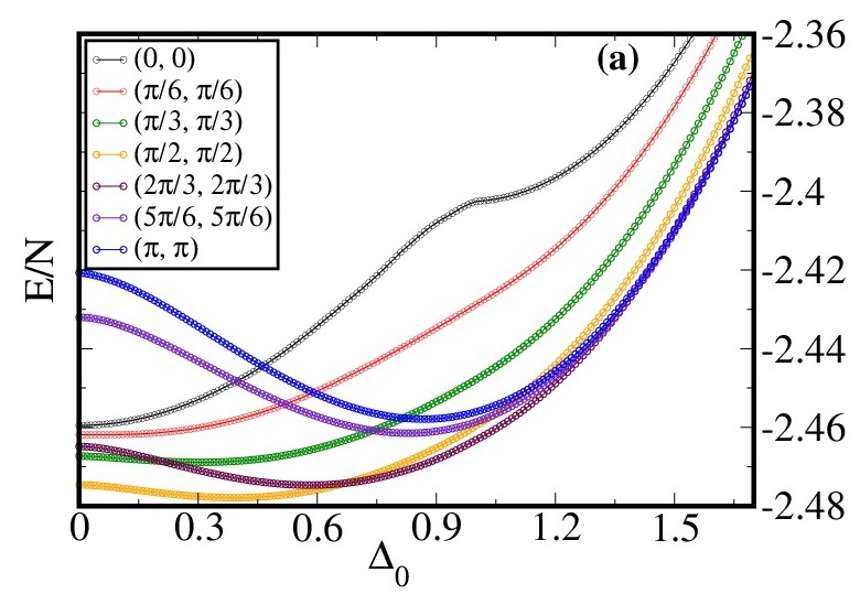
We will discuss the general features further on and for the moment focus on $E(\Delta_{0},{\bf q})=\langle H_{eff}(\Delta_{0},{\bf q})\rangle$ at a typical parameter point: $U=4t$, $J=t$ and $\mu=-2t$ (corresponding roughly to $n=0.4$), in Fig.1. The figure shows the variation of the energy with respect to $\Delta_{0}$ for different choices of ${\bf q}$ (covering panels (a) and (b)) and the absolute minimum defines the appropriate magnetic-superconducting state. The ground state phase diagram is established by carrying out this exercise for different $\mu$, $J$ and $U$.

Given our parametrisation of the variational state, we always have magnetic order with some ${\bf Q}$ (where ${\bf Q}$ denotes the optimized value of ${\bf q}$), while superconducting order is absent if the optimum $\Delta_{0}=0$.

 

Figure 3: Color online: Ground state $n-J$ phase diagrams showing evolution of the magnetic and superconducting phases for three values of $U$. (a) The purely magnetic phase diagram at $U=0$. The magnetic phase changes with the filling but the order of the occurrence of phases remains unchanged with varying $J$. (b) At $U=2t$ superconductivity is seen over a $J$ window that widens with increasing $n$. The magnetic phases remain roughly as they were at $U=0$. (c) At $U=4t$ the superconducting window is wider, and the magnetic phases near $n=1$ are modified although elsewhere it looks roughly similar to the small $U$ picture. There is a tiny window of modulated superconducting order (FFLO) state, in the bottom left corner of the finite $U$ phase diagrams (see text) but they are almost invisible on the $n-J$ scales used here.

III.1.2 Variation of pairing field and magnetic order

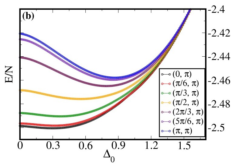
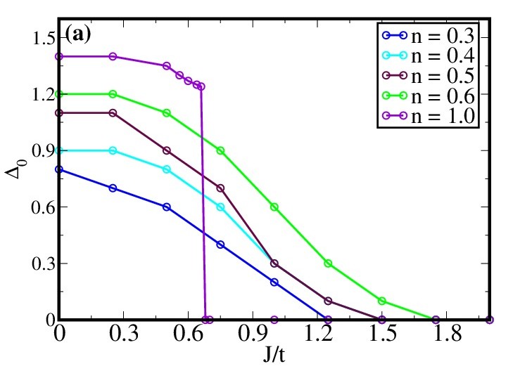
Tracking the minimum for varying $\mu$ and $J$ leads to the ground state parameters shown in Fig.2. Over the $J$ range that we explore the density $n(\mu,J)$ (to an accuracy $\sim 0.01$) is almost independent of $J$ at fixed $\mu$. That allows us to phrase the results in terms of $n$, although the minimization was done at fixed $\mu$ and $J$. Fig.2(a) shows the $J$ dependence of the pairing field amplitude at several values of $n$. The results here are for $U=4t$, we will discuss the phase diagram at other values of $U$ later.

Increase in magnetic coupling suppresses the pairing field amplitude. At a scale $J_{c}(n)$ the pairing amplitude vanishes, indicating the destruction of the superconducting phase. We make a few observations: (1) $J_{c}(n)$ vanishes as $n\rightarrow 0$, and it increases with $n$ with a maximum at $n\sim 0.6$ at $U=4$. This maximum, $J_{c}^{max}$, $\sim 1.5t$. (2) The critical value at $n=1$ is much smaller, with $J_{c}(n=1)\sim 0.75t$. (3) The transition with increasing $J$ is first order at $n=1$ and second order for $n\neq 1$.

Fig.2(b) and 2(c) shows the components of the corresponding magnetic wave vectors. In the absence of pairing, and at low $J$, the magnetic order is decided by the RKKY interaction, with the peak in the band susceptibility $\chi_{0}({\bf q})$ dictating the ordering wavevector ${\bf Q}$. At larger $J$ the spiral states gradually give way to collinear phases and finally to just two phases, ferromagnetic and Neel, with a window of phase separation in between. In the presence of a pairing interaction it is not essential that the same trend be followed but, as pointed out long back by Anderson and Suhl and-suhl , the presence of pairing affects the electronic density of states only over a window $2\Delta_{0}\ll\epsilon_{F}$ so except for ${\bf q}\rightarrow 0$ the spin susceptibility is mostly unaffected.

Our results are at $U=4t$ with the pairing field $\Delta_{0}\sim t$ so the density of states is affected over a fairly wide window. Nevertheless, except near $n=1$, the RKKY trend still holds at small $J$. The phase diagrams in Fig.3 quantify these further.

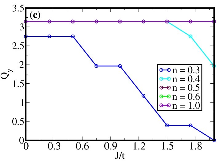
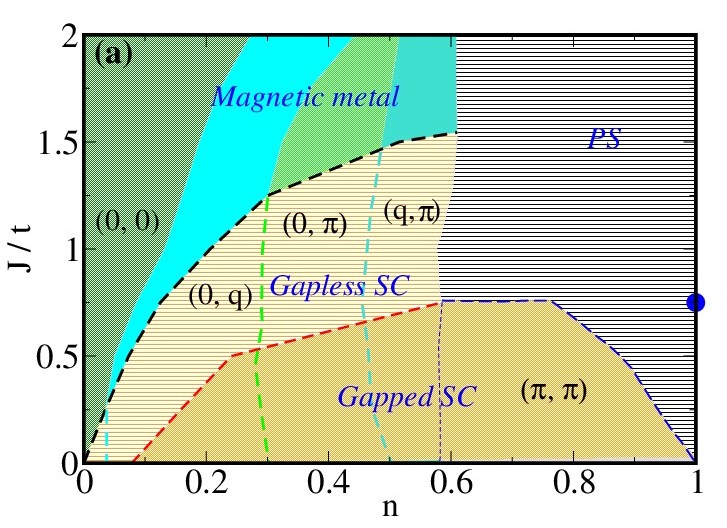
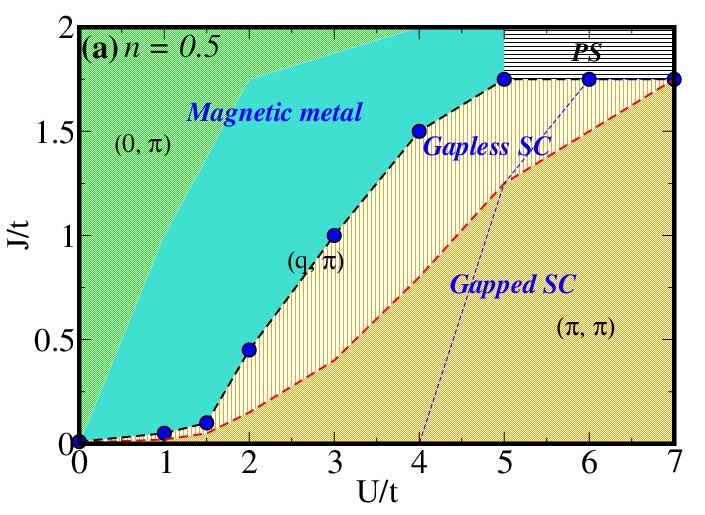
III.1.3 $n-J$ phase diagrams

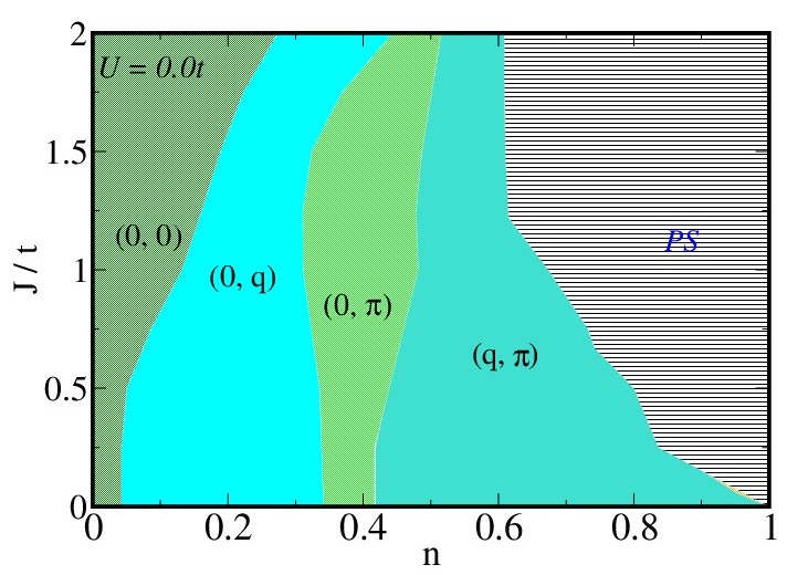
Fig.3 shows the ground state phase diagram obtained through our variational calculations. The $U=0$ situation, panel (a), corresponds to just the classical Kondo lattice in two dimensions. With respect to this non superconducting reference, (b) and (c) show the impact of increasing pairing interaction on the magnetic state as well as the increasing window of superconducting order. We discuss the three cases separately.

(i) No pairing interaction $(U=0)$: In this case $\Delta_{0}=0$ and the ground state is characterized only by ${\bf Q}$. We discuss the $J/t\rightarrow 0$ and the $J/t\gtrsim 1$ limits separately.

The small $J/t$ limit is controlled by the RKKY interaction with the effective spin-spin coupling being $J_{ij}\propto J^{2}\chi^{0}_{ij}$, where $\chi^{0}_{ij}$ is the non local band susceptibility of the conduction electrons. The ordering wavevector is dictated by the maximum in $\chi^{0}({\bf q})$, the Fourier transform of $\chi^{0}_{ij}$. This depends on $\mu$, or the filling $n$. The system evolves from a ${\bf Q}=\{0,0\}$ (ferromagnet) at low filling, to a $\{0,q\}$ phase at the intermediate filling. Further increase in filling leads to a $\{0,\pi\}$ antiferromagnet, followed by a $\{q,\pi\}$ phase and then to a $\{\pi,\pi\}$ Neel antiferromagnet at half filling $n=1$. There are no phase separation windows in the $J/t\rightarrow 0$ limit and all transitions are second order.

For $J/t\gtrsim 1$ the sequence of magnetic phases, with increasing filling, remains the same as at weak coupling but the window of spiral states shrink yielding to the FM state at low density and a window of phase separation near $n=1$. For $J/t\gg 1$ (not shown in the figure) the only surviving states are the ferromagnet and the $n=1$ Neel state, separated by a phase separation window. The system heads towards the ‘double exchange’ limit.

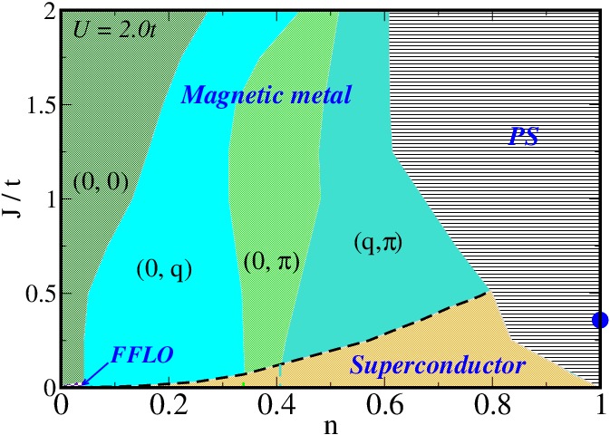
(ii) Weak attraction $(U\sim t)$: On a finite lattice the finite size gap $\sim t/L^{2}$ (in 2D) makes it difficult to stabilize a superconducting state below a $L$ dependent scale. Since we are using a real space framework, to connect up with finite $T$ Monte Carlo calculations later, we have only limited data at $U<2t$. Fig.3(b) shows results at $U=2t$ as typical of ‘weak coupling’.

At $U=2t$ and $J=0$ we have the usual ${\bf k},\uparrow,~{}-{\bf k},\downarrow$ pairing. At finite $J$ one would (a) expect the magnetic order to be modified since the effective spin-spin interaction is now in a finite $\Delta_{0}$ background, and (b) the superconductivity to be weakened since the pairing is no longer between ${\bf k},\uparrow,~{}-{\bf k},\downarrow$ but the states ${\bf k},{\uparrow}$ and $-{\bf k}+{\bf Q},{\downarrow}$, where ${\bf Q}$ is the magnetic ordering vector.

The first effect is weak since the maximum $\Delta_{0}\sim 0.4t$, opening only a modest gap in the density of states with limited impact on the spin-spin interaction. So the magnetic character within the superconducting window, Fig.3(b), is very similar to the $U=0$ case. The $\Delta_{0}$ however falls with increasing $J$, surviving to a scale $J_{c}(n)$ shown in the panel. The maximum of $J_{c}$ occurs at $n\sim 0.8$ and the value at $n=1$ is lower than that. In the regime $\Delta_{0}=0$ the magnetic phases are of course as in panel (a).

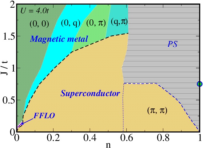
(iii) Intermediate attraction $(U\gg t)$: Panel (c) shows data at $U=4t$ and the $\Delta_{0}$ at $n\sim 0.8$ is now $1.4t$, much larger than at $U=2t$. As a result, the electronic density of states is modified with respect to its band character over a wide energy window.

Figure 4: Color online: Electronic density of states at different filling and magnetic coupling at $U=4t$, on magnetic-superconducting backgrounds obtained through the variational scheme. For $n=0.3$ (panel (a)) and $n=0.5$ (panel (b)) the DOS shows transition from a gapped to a gapless superconducting state at some coupling $J_{g}(n)$. At $n=1$ the system remains gapped throughout, however, there is a nonmonotonicity in the behavior of the gap as one transits from the magnetic superconductor to the magnetic insulator at a critical value $J_{c}\sim 0.75t$.

The changed density of states changes the spin-spin coupling and the magnetic phases show clear differences with respect to the small $U$ cases. These include changes in the magnetic phase boundaries within the SC phase and the emergence of a window of Neel order with ${\bf Q}=(\pi,\pi)$, close to $n=1$.

Superconducting order survives over a wider range of magnetic coupling with the maximum $J_{c}$ being $\sim 1.5t$, occurring at $n\sim 0.6$. Beyond $n\sim 0.6$ there is a quick drop in $J_{c}$ as a phase separation window intervenes. The $J_{c}$ at $n=1$ is $\sim 0.75t$, well below the maximum at $n\sim 0.6$.

III.2 Quasiparticle properties

The magnetic superconducting state involves a suppression of $\Delta_{0}$ as $J$ increases. Had the pairing been between the usual $|{\bf k}\uparrow\rangle$ and $|-{\bf k}\downarrow\rangle$ states it would have led to a suppressed BCS gap with the overall character of the density of states (DOS) remaining unchanged. However, the pairing now takes place in a magnetic background, where the Bloch states are superposition of $|{\bf k}\uparrow\rangle$ and $|{\bf k}+{\bf Q}\downarrow\rangle$. The combination of pairing and magnetic interaction now connect a larger set of states. For example $|{\bf k}\uparrow\rangle$ connects to $|{\bf k}+{\bf Q}\downarrow\rangle$, $|-{\bf k}-{\bf Q}\uparrow\rangle$, and $|-{\bf k}\downarrow\rangle$. The eigenspectrum that emerges need no longer look like the ‘BCS’ result. In the section below we describe the features that we observe and in the section after we try to analyze these features in terms of the approximate Green’s function theory.

Figure 5: Color online: (a) Gap in the DOS plotted as a function of magnetic coupling for different fillings. At $n=1$ for $J\leq 0.9t$ the superconducting gap gets progressively suppressed with $J$. Beyond $J\sim 0.9t$ the gap is the antiferromagnetic gap which increases with $J$. At $n\neq 1$, the gap reduces monotonically with $J$, in agreement with $\Delta_{0}$ (see Fig.2a). (b) $n-J$ phase diagram at $U=4t$ showing the gapped and gapless superconducting phases.

III.2.1 Density of states

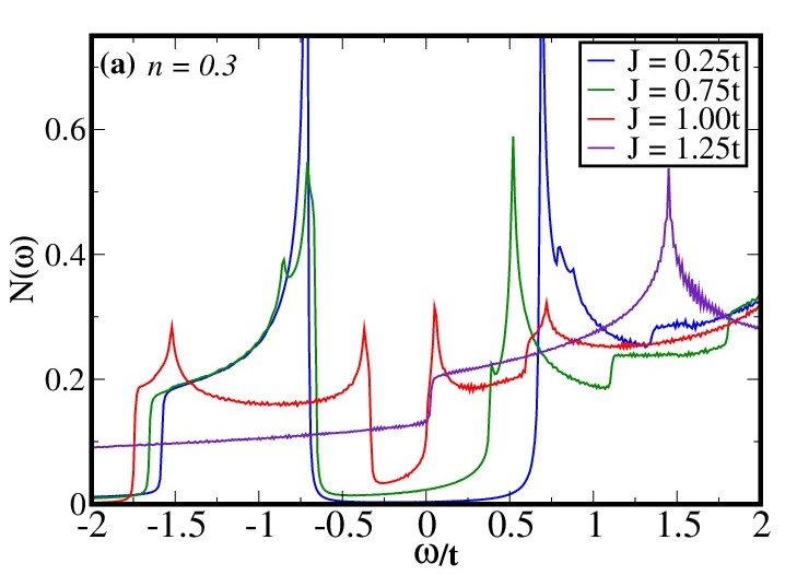
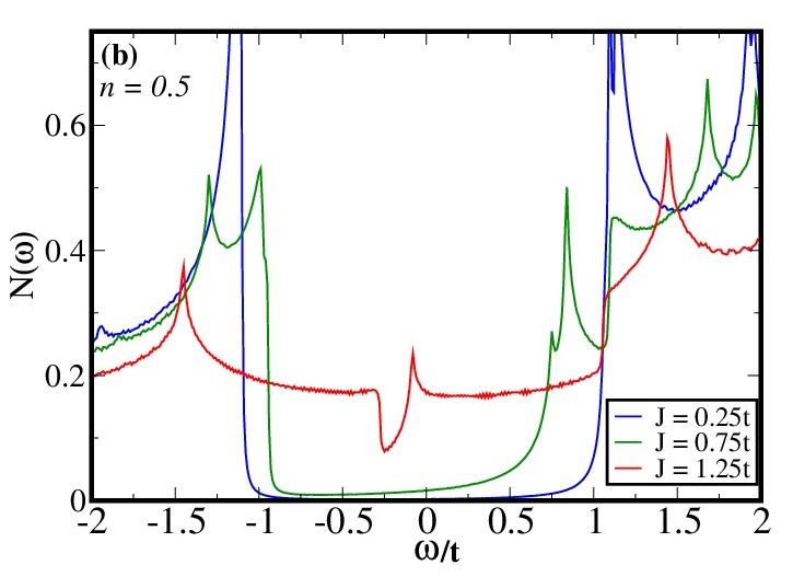
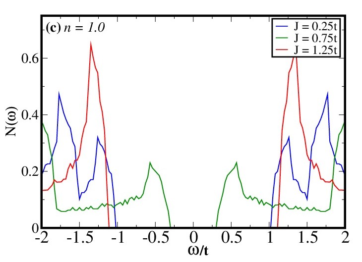
Fig.4 shows the electronic DOS computed on backgrounds obtained through the Green’s function calculation. The three panels comprise of DOS pertaining to three density regimes and varying $J$. The attractive interaction is $U=4t$ in all cases.

Figure 6: Color online: The spin summed electron spectral function, $A({\bf k},\omega)$ for ${\bf k}$ varying from $(0,0)$ to $(\pi,\pi)$ at different combinations of $n$ and $J$ and $U=4t$. At $n=1$ (top row) the gap near $(\pi/2,\pi/2)$ reduces from $J=0.25t$ to $J=0.75t$ but increases again at larger $J$. There are also multiple bands visible at $J=0.25t,~{}0.75t$. At $n=0.5$ and $n=0.3$ the low $J$ result is almost BCS like, with only two bands visible, while the $J=0.75t$ case shows a large number of bands, with one crossing $\omega=0$. At larger $J$, as $\Delta_{0}$ becomes very small, the bandstructure simplifies again and is mostly described by the ‘magnetic metal’ limit. The results are shown for $36\times 36$ lattice.

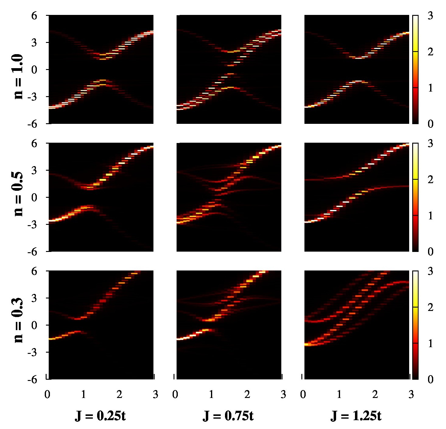
Fig.4(a) shows the situation at filling $n=0.3$. The spectrum remains gapped at weak $J=0.25t$ (modulo a ‘tail’ due to the lorentzian broadening) and has the usual gap edge singularities akin to the $J=0$ case. At $J=0.75t$, however, there is finite DOS at $\omega=0$ and the remnant of the ‘gap edges’ have moved inward. The inward movement of the edges can be attributed to the reduced $\Delta_{0}$ as $J$ increases but the low energy DOS involves a new band. $J=t$ shows even larger DOS at $\omega=0$ and makes visible new van Hove singularities. The understanding of these features come from an analysis of the dispersion using the momentum resolved spectral functions. We take that up in the next section and just highlight the features in the changing DOS here.

Figure 7: Color online: Low energy spectral weight at the Fermi level for different $n-J$ cross sections. The parameters are the same as in Fig. 6. An weak $J/t$ give rise to a gapped state and consequently there is no low energy weight near the Fermi level. Increase in $J/t$ leads to pile up of spectral weight near the Fermi level whose symmetry is dictated by the underlying magnetic wave vector ${\bf Q}$. The distribution of the spectral weight near the Fermi level is anisotropic, indicative of a nodal Fermi surface.

At $n=0.5$ the observations are qualitatively similar to the $n=0.3$ case, with finite DOS at $\omega=0$ being visible at the two upper values of $J$. The overall ‘gap structure’ within which the low energy features are seen is wider at $n=0.5$ due to the larger $\Delta_{0}$.

The behavior at $n=1$, Fig.4(c), is distinctly different. The presence of satellite peaks within the BCS like gap is significant in this case. The spectrum is gapped at all magnetic coupling but the gap shows nonmonotonic behavior. Initially increase in magnetic coupling pushes the satellite peaks to low energy narrowing the gap. However the pairing amplitude itself vanishes at a critical $J\sim 0.75t$, beyond which the system changes to a magnetic insulator - with the gap now being proportional to and sustained by $J$.

III.2.2 Gapped and gapless regimes

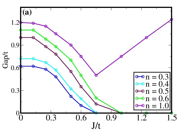
Fig.5(a) shows the $J$ dependence of the gap at different filling. At weak magnetic coupling the superconducting gap follows the behavior of the pairing field amplitude and undergoes suppression with increasing $J$. At half filling, till a coupling of $J\sim 0.9t$ the behavior of the gap is the same as that of its low filling counterpart. For $J\gtrsim 0.9t$ the gap increases linearly with $J$. The gap in this regime arises from antiferromagnetic ($\pi,\pi$) order. For $n\neq 1$ the gap vanishes at a scale we call $J_{g}(n)$.

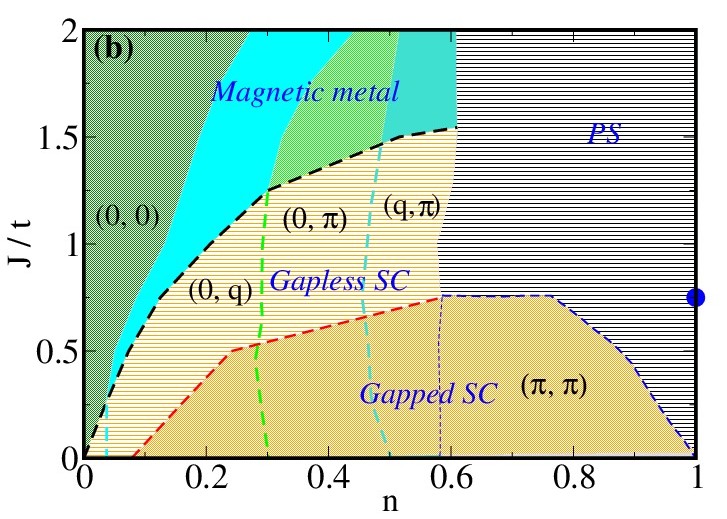
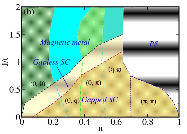
Fig.5(b) shows the $n-J$ phase diagram at $U=4t$, now with the superconducting phase demarcated into gapped and gapless regimes. The gapped regime is characterized by the presence of large $\Delta_{0}$ while the gapless window has relatively smaller $\Delta_{0}$. That by itself does not explain why the qualitative character of the DOS changes, so we examine the electron dispersion in the magnetic superconductor to explore this issue.

III.2.3 Electron dispersion

Fig.6 shows the momentum resolved spectral function $A({\bf k},\omega)=\sum_{\sigma}A_{\sigma}({\bf k},\omega)$ for three different $n-J$ combinations. The momentum scan is along the diagonal of the Brillouin zone, ${\bf k}=(0,0)\rightarrow(\pi,\pi)$. Since the spectra are computed on an ordered state there is no broadening of the lines and we essentially map out the multi-branch dispersion in the magnetic-superconducting state.

We begin with $n=1$, top row. At weak magnetic coupling, $J=0.25t$, the behavior is BCS like with the characteristic back bending feature in the dispersion curves. The effective gap is slightly reduced compared to its BCS value, and there is a small branching visible for ${\bf k}\sim(\pi/2,\pi/2)$. At $J=0.75t$ the branching feature is far more prominent and the separation between the inner branches, that sets the gap, is much smaller than at $J=0.25t$. ${\bf k}$ regions associated with ${\partial E_{\alpha}({\bf k})}/{\partial{\bf k}}=0$, where $E_{\alpha}({\bf k})$ are the dispersion, lead to the van Hove singularities observed in Fig.4(c).

At $n=0.5$, middle row, weak $J$ essentially reproduces the BCS result, with a smaller gap than $n=1$ due to the smaller $\Delta_{0}$ - occurring at a lower ${\bf k}$ due to the lower filling. At $J=0.75t$ a very complex picture emerges, with in principle all the 8 bands that arise from BdG being visible (although a six band, Green’s function based, approach captures the essential features). Along the $(0,0)\rightarrow(\pi,\pi)$ scan one of the bands seems to cross $\omega=0$. The multiple and prominent $E_{\alpha}({\bf k})$ generate the van Hove singularity structure seen in Fig.4(b). At $J=1.25t$ the $\Delta_{0}$ is very small and the features are similar to that of a magnetic metal.

At $n=0.3$ the qualitative features are similar to $n=0.5$ although the multiple bands are not all visible for the color scheme that we have used. The superconducting state survives to $J_{c}\sim t$ and the $J=1.25t$ result is for a magnetic metal.

While it is difficult to extract useful analytic expressions for the three branches of the dispersion from each $G_{\sigma\sigma}({\bf k},\omega)$, explicit functional forms can be obtained in the gapless phase when $\Delta_{0}\lesssim J$. We provide these results in the Appendix, and have cross checked them with respect to the numerical results.

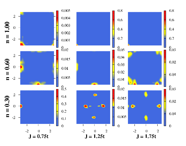
III.2.4 Low energy weight distribution

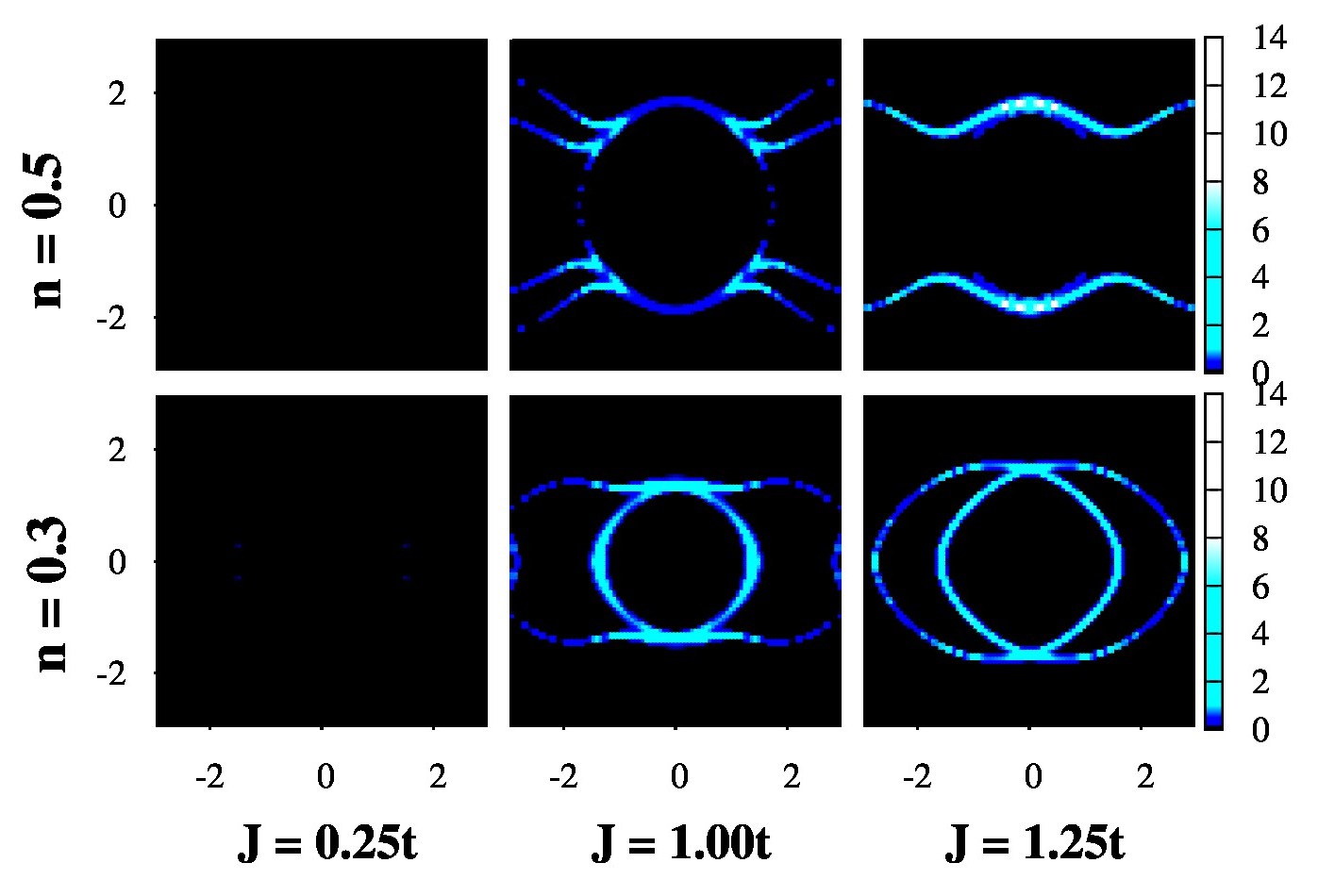
In connection to the spectral features discussed above in Fig.7 we show the distribution of low energy spectral weight across the Brillouin zone at low and intermediate filling (at $n=1$ the spectrum is always gapped). At weak magnetic coupling the spectrum is gapped out and thus there is no low energy weight.

We computed the ${\bf k}$ dependent spectral weight at $\omega=0$, summed over spin channels, $A({\bf k},0)=\sum_{\sigma}A_{\sigma\sigma}({\bf k},\omega)$, where:

$$A_{\uparrow\uparrow}({\bf k},0) = -(1/\pi)Im~{}{1\over{i\eta-(\epsilon({\bf k})-\mu)-\Sigma_{\uparrow\uparrow}({\bf k},i\eta)}}|_{\eta\rightarrow 0}$$ (12)

(13)

(14)

$$\Sigma_{\uparrow\uparrow}({\bf k},i\eta) = {\Delta_{0}^{2}\over{i\eta+(\epsilon({\bf k})-\mu)}}+{J^{2}\over{i\eta-(\epsilon({\bf k}+{\bf Q})-\mu)}}$$

etc. The results in Fig.7 highlight the rather strange looking ‘Fermi surface’ that emerge. The low $J$ panels show no spectral weight since the system is gapped. $J=t$ shows non trivial Fermi surfaces in the superconductor, dictated by the magnetic wavevector, while $J=1.25t$ is superconducting for $n=0.5$ and a magnetic metal for $n=0.3$.

IV Discussion

This section covers some issues of method, related to the approximations that we have made in handling the model in Eqn.1, and the phase diagram, in terms of the magnetic coupling and attractive interaction. We comment on what it suggests for spectral features in the borocarbides.

IV.1 Computational issues

IV.1.1 The ‘classical’ approximations

The model in Eqn.1 involves an attractive electron-electron interaction $U$ and the coupling $J$ between the electron spin and a local moment of spin $S$. This describes interactions between quantum degrees of freedom, and, beyond weak coupling, is very non trivial. The treatment of the Hubbard interaction in terms of a classical pairing field, and of the spin $S$ as classical, makes the model tractable by reducing it to a variational problem determining a static $\{\Delta_{i},{\bf S}_{i}\}$ background that minimizes the electron energy.

Figure 8: Color online: Magnetic structure factor at $T\sim 0$ for different filling and magnetic interaction $J$. At half filling ($n=1$) the MC always leads to a ${\bf Q}=(\pi,\pi)$, Neel, state, as in the VC. At the intermediate filling of $n=0.6$ a $(0,\pi)$ and a $(q,\pi)$ state is realized for the particular choice of the magnetic coupling, in agreement with the VC results. At low filling of $n=0.3$ and intermediate and strong magnetic coupling the state as obtained through MC slightly deviates from that obtained through the VC, with the $(0,q)$ being now replaced by $(0,\pi)$, the neighboring phase in the VC phase diagram.

The mean field approximation for $U$ makes qualitative sense as long as $\Delta_{0}\neq 0$. The presence of superconducting order at $J=0$ is well known, the persistence of order at small $J$ has also been established via numerically exact methods. This suggests that the mean field treatment of $U$ is a valid first approximation. Quantum fluctuations of the pairing field would be important near $J_{c}$ in the large $U$ problem, where the mean field amplitude vanishes, but correlation effects would be significant. We have not focused on that regime here.

The treatment of the local moment as ‘classical’ is valid when $2S\gg 1$. For the borocarbides $4f$ shells for the magnetic superconductors involve $2S\sim 3-5$ and the classical treatment again ought to be reasonable. There are, however, low moment, and non magnetic, superconductors involving Tm and Lu which cannot be captured well within our scheme.

IV.1.2 Single -vs- multichannel decomposition of interaction

We have considered the effect of $U$ only in the pairing channel, and the magnetic response arises from the ${\bf S}_{i}$. As a first approximation this is justified because the pairing and magnetic effects arise from different couplings in our model (the $U$ is not primarily responsible for the magnetic order). However, there would be a renormalisation in the magnetic sector arising from the $U$, if we were to consider an additional magnetic decoupling of the Hubbard term. We discuss this below.

Figure 9: Color online: The ground state $n-J$ phase diagram as obtained through MC (right) in comparison to the one obtained through the variational calculation (left) at $U=4t$. Notice that the gapless regime shrinks in the MC phase diagram as compared to the one obtained through VC. The emergence of the Neel, $(\pi,\pi)$ antiferromagnetic window near $n=1$ is verified through the MC as well.

Decomposing $U$ in both the magnetic and pairing channels lead to the effective Hamiltonian,

$$H = H_{kin}+H_{pair}-\sum_{i}\{(JS_{i}^{+}-h_{i}^{+})\sigma_{i}^{-}+h.c\}$$

$$~{}~{}~{}~{}~{}~{}~{}~{}~{}~{}~{}~{}~{}~{}~{}~{}~{}~{}~{}~{}~{}~{}~{}~{}+|U|\sum_{i}\{|\Delta_{i}|^{2}+\langle\sigma_{i}^{+}\rangle\langle\sigma_{i}^{-}\rangle\}$$

where, $h_{i}^{+}=U\langle\sigma_{i}^{+}\rangle$ and $\sigma_{i}^{+}=c_{i\uparrow}^{\dagger}c_{i\downarrow}$, etc. For $h_{i}^{+}=U\langle\sigma_{i}^{+}\rangle$ to be nonzero does not require symmetry breaking driven by $U$. There is a ‘source term’, since $JS_{i}^{-}$ already forces $\langle\sigma_{i}^{+}\rangle\neq 0$. So, the leading effect of the magnetic decoupling can be estimated simply by calculating $U\langle\sigma_{i}^{+}\rangle_{0}$, where the subscript zero refers to the model with only pairing decomposition.

We have checked that the ‘original’ exchange field $JS_{i}^{+}$ and the renormalised field $JS_{i}^{+}-U\langle\sigma_{i}^{+}\rangle_{0}$ have the same spatial character, so the leading effect of the magnetic channel can be included via a renormalisation $J\rightarrow J_{eff}$. The effective exchange field is smaller than the bare field by $15-20\%$, which we think arises due to the diamagnetic tendency of the attractive $U$ term. The weaker $J_{eff}$ will expand the domain of superconducting order marginally without affecting any qualitative conclusion.

IV.1.3 Comparison with unrestricted minimization

Fig.8 shows the magnetic structure factor computed at different filling for three different regimes of the magnetic interaction. In the intermediate and strong coupling regimes, cooling down the system from an uncorrelated high temperature state reproduces the magnetic order as has been obtained through the variational calculations. In the weak interaction regime however, the system fails to attain the global minimum in the energy landscape within the limited annealing time and finite system size. The configuration thus obtained through the Monte Carlo is often energetically unfavorable compared to the one obtained variationally. Nevertheless, over a wide parameter space the variational ground state is well reproduced on cooling down from a high temperature state.

The resulting ground state phase diagram is shown in Fig.9, in comparison to the one obtained through the variational scheme. The ground state as obtained through the Monte Carlo certainly agrees qualitatively with all features of the variational result, and also confirms that the ‘homogeneous’ $\Delta_{i}$ assumption for the ground state is not unreasonable.

IV.1.4 Coexistence of modulated pairing order with ferromagnetism

Our variational calculation suggests that a homogeneous superconducting state cannot coexist with a large ferromagnetic internal field $JS$. However, it is known fflo_assort ; mpk_bp that homogeneous superconducting order can exist in the presence of a weak external magnetic field, beyond which there is a narrow regime of modulated Fulde-Ferrell-Larkin-Ovchinnikov (FFLO) order, before pairing is lost. This effect does exist in our phase diagram as well, but over a very narrow window so it has not been given prominence in Fig.3. We comment on this below.

For a superconductor in an applied field $h$, the FFLO state exists over a window $h_{1}(n)$ to $h_{2}(n)$ fflo_assort ; mpk_bp . Below $h_{1}$ the system remains a homogeneous superconductor, with zero spin polarization. This is traditionally called the ‘unpolarised superfluid’ (USF) state. Above $h_{2}$ the system is a magnetized normal Fermi liquid. The equivalent in our model are two magnetic couplings $J_{1}(n)$ and $J_{2}(n)$. Knowing $h_{1}(n)$ and $h_{2}(n)$ one can just superpose these on the ferromagnetic window of the $n-J$ phase diagram to locate the USF and FFLO regimes. Fig.3 shows these tiny windows, virtually invisible at $U=2t$. The reason the window is so small is due to the tiny density window over which ferromagnetism shows up at small $J$, and the small $J_{1}$ and $J_{2}$ scales in the small $n$ window. $J_{1}$ and $J_{2}$ are related to the pairing gap in the spectrum, and this vanishes as $n\rightarrow 0$.

In summary, a local moment polarized homogeneous superconductor, and a pair modulated ferromagnetic state, can exist in our model, but over a tiny density and $J$ window.

IV.1.5 Size limitations

The variational calculation, when cast in momentum space, does not have significant size limitations, except in the number of ${\bf q}$ values over which the energy has to be minimized.

A more serious size limitation arises when Monte Carlo based simulated annealing is used for ‘unrestricted’ minimization, and for accessing finite temperature properties. This requires iterative diagonalization of a $4N\times 4N$ matrix (where $N=L^{2}$) and even when a cluster algorithm is used for the MC updates only sizes upto $24\times 24$ can be accessed within reasonable time. We have checked that thermodynamic properties can be accessed down to $U=2t$ reliably on these sizes, but the subtle spectral features that one observes in the large size ground state calculations cannot be resolved well on these sizes. We also cannot go down to $U\sim t$, which we believe is appropriate for quantitative description of the borocarbides.

IV.1.6 Benchmarking the Green’s function results

The BdG problem generates 8 bands for a given ${\bf k}$ since each $|{\bf k}\sigma\rangle$ connects to three other states via pairing and magnetic scattering, and the results for $\sigma=\uparrow$ and $\sigma=\downarrow$ are now non degenerate. Some of the residues associated with these bands can, however, be quite small and hard to identify. The Green’s function approach on the other hand truncates the scattering processes to $J^{2}$ and $\Delta_{0}^{2}$, dropping $J^{2}\Delta_{0}^{2}$, and the resulting Green’s function has three poles for each ${\bf k}\sigma$. The results are obviously exact at $J=0$ or $\Delta_{0}=0$, but, as the results in Fig.10 show, they are surprisingly accurate over a large $\Delta_{0}-J-n$ parameter range.

The results however are not accurate for the magnetic superconductor at $n=1$ where an unusual DOS emerges (see Fig.4(c)) and also at low $J$ at other densities where a spurious low energy band with a small residue, $\propto J^{2}$, emerges. Away from these parameters the Green’s function approach provides a useful tool for understanding the complex band structure.

Figure 10: Color online: Comparison of the total spectral function $A({\bf k},\omega)$ obtained from the BdG diagonalization and the Green’s function method, for parameters mentioned in the figure. The top row in each set corresponds to the BdG results while the bottom row shows the Green’s function result. The agreement is reasonable for all the parameters shown here. The results here are at $U=4t$ and for momenta discretised on a $36\times 36$ lattice.

Figure 11: Color online: Top row: Electronic density of states for the square lattice on two different magnetic backgrounds and varying $J$, at $n=0.5$. Bottom row: Same as above for a three dimensional (cubic) lattice, for the choice of the magnetic wave vectors shown in the individual panels. The DOS are computed through the Green’s function method for a pairing field amplitude of $\Delta_{0}=0.2t$, plausible for a weak interaction regime. In both 2D and 3D the system undergoes transition from a gapped to a gapless state with increasing magnetic coupling.

IV.1.7 Extension to low $U/t$

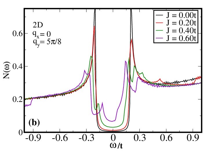
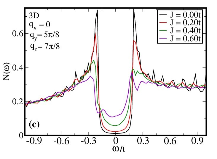
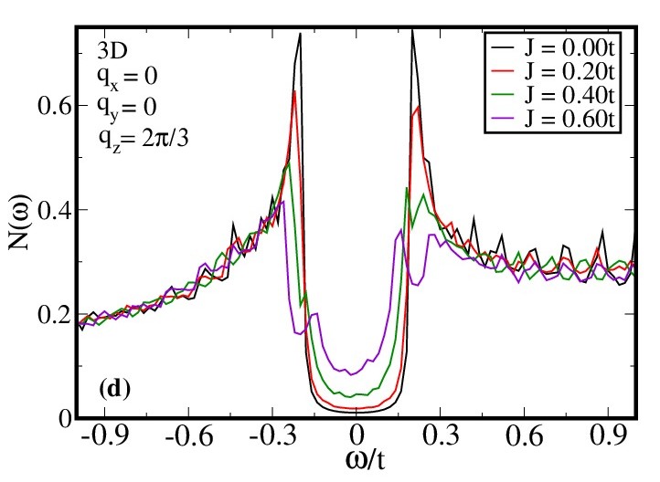
Since the thermal physics cannot be worked out on lattices beyond a certain size (say with $N_{max}\sim 30\times 30$) we have restricted our study mainly to $U\gtrsim 2t$. However it is worth exploring if a gapless superconducting phase can arise at much lower $U$, and therefore much smaller $\Delta_{0}$, than we have studied till now. This will be relevant for real materials which are mainly in the weak coupling, $U\lesssim t$, limit. In Fig.11(a) and 11(b) we show the DOS calculated through the Green’s function method for typical spiral magnetic backgrounds, with ${\bf Q}$ marked in the Fig, and pairing field amplitude set to $\Delta_{0}=0.2t$. We study both the two dimensional and three dimensional case (which is experimentally more relevant) and find that all cases show a gapped to gapless transition with increasing $J$ on a scale $J_{g}\sim\Delta_{0}$.

This little demonstration is just meant to emphasize that the occurrence of a gapless phase at finite $\Delta_{0}$ is not an artifact of large $U$ or two dimensionality and can well occur in weak coupling 3D superconductors as well.

IV.2 Relating to experiments

IV.2.1 $U-J$ phase diagram

The results at $U=4t$ are part of a larger $U-J-\mu$ phase diagram. In real solids the attractive interaction would be typically much smaller that $4t$ (and in possible cold atomic systems they could be larger). Keeping this in mind we attempted to map out the $U-J$ phase diagram at a few densities. Fig.12, top row, shows our results at $n\sim 0.5$ and $n\sim 0.3$.

We find the following: (i) At $n\sim 0.5$ over the range of $U$ the system exhibits G-type antiferromagnetic order ($\pi,\pi$) or ($q,\pi$) order depending upon $J$. The superconducting phase makes a gapped to gapless transition at a $J$ that increases with $U$. (ii) At $n=0.3$ the magnetic state can be ($\pi,\pi$), ($q,\pi$) or ($0,\pi$). The superconducting state is gapped or gapless depending upon the strength of the magnetic interaction, with the large $U\gg J$ regime favoring gapped superconductivity. The $J\gtrsim U$ regime again gives rise to gapless SC and finally a magnetic metal. No phase separated regime is realized at low filling.

Figure 12: Color online: (a)-(b) Ground state $U-J$ phase diagram at $n\sim 0.50$ (panel (a)) and $n\sim 0.3$ (panel (b)). (c) Organization of the borocarbide ground state in terms of the de Gennes (DG) factor, ${S(S+1)}$, denoting the strength of local electron-spin coupling, and the Hopfield parameter, $\eta$, indicative of the strength of pairing interaction. The DG factor is like our $(JS)^{2}$, while $\eta$ relates to $U$.

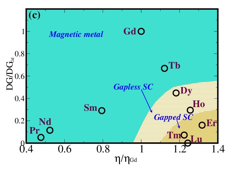
IV.2.2 The borocarbide phase diagram

In the borocarbides neutron scattering experiments reveal the nature of magnetic order. There is an overall similarity in the order as one goes down from GdNi₂B₂C, where the DG factor is largest, to TmNi₂B₂C, where the DG factor is smallest, through DyNi₂B₂C, HoNi₂B₂C, etc. All of them seem to have a ${\bf Q}=(0,0,q)$ pattern of ordering, with $q\sim 0.55$. The order is ferromagnetic in the basal plane with a spiral along the $c$-axis lynn1997 .

Two material parameters are believed to be important in these compounds. They are (i) the de-Gennes factor (DG) that we have already introduced, proportional roughly to our $(JS)^{2}$, and (ii) the ‘Hopfield parameter’, $\eta$, defined michor2000 as, $\eta=N(E_{F})\langle I_{\alpha}^{2}\rangle$, where $\langle I_{\alpha}^{2}\rangle$ is average of the electron-phonon matrix element over the atoms R, Ni, B, C, and $N(E_{F})$ is the DOS at the Fermi level. $\eta$ relates roughly to $U$ in our case. Both DG and $\eta$ have been tabulated for the borocarbides.

Figure 13: Color online: $J-T$ phase diagram at $n=0.5$. Magnetic coupling strongly suppresses the superconducting $T_{c}$ and at intermediate coupling there is coexistence of the magnetic and superconducting order. In addition to the superconducting $T_{c}$ we show a magnetic scale $T_{AF}$ below which the correlation length grows exponentially (but there is no true long range order since we are in two dimensions). A third scale, $T_{g}$, showing the transition from a gapped to a gapless superconducting phase, emerges.

We organized the experimental phase diagram of the borocarbides in terms of $\eta$ and DG (normalizing by the value for Gd), Fig.12.(c), and compare it with our variational $U-J$ phase diagram at a typical density $(n=0.5)$ in Fig.12.(d). For the real materials the magnetic and superconducting boundaries are well established but the possible ‘gapped to gapless’ boundary that we show in 12.(c) is our conjecture based on 12.(d). We believe that unless the ‘multiband’ character of the real materials invalidates the basic picture there must be an increase in the gap anisotropy (if not a gapless state) as one moves to increasing DG from Er $\rightarrow$ Ho $\rightarrow$ Dy, before superconductivity is lost in Tb. There is indeed some evidence for gap anisotropy and nodal quasiparticles in the borocarbides, we review that quickly below.

The borocarbides studied involve two ‘non magnetic’ compounds, YNi₂B₂C and LuNi₂B₂C (which do not have local moments), in addition to those with finite $4f$ moment and DG factor. Among both the non magnetic and magnetic superconductors one observes an apparent direction dependence of the gap on the Fermi surface canfield2003 ; izawa2002 ; takagi2004 ; shin2010 ; baba2008 ; rybaltchencho1999 ; yanson2008 ; schultz2011 .

In case of YNi₂B₂C and LuNi₂B₂C scanning tunneling spectroscopy (STS) canfield2003 , c-axis thermal conductivity izawa2002 , ultrasound attenuation takagi2004 , etc., suggest that the superconducting energy gap is of the anisotropic s-wave type, with point nodes along [100] and [010]. The tunneling current in STS canfield2003 as well as the $\sqrt{H}$ dependence of finite field heat capacity izawa2002 suggests the presence of low energy quasiparticles. Angle resolved photoemmission spectroscopy (ARPES) on YNi₂B₂C suggests shin2010 that different parts of the Fermi surface contributes differently towards to superconductivity. These ‘non magnetic’ compounds are expected to have strong antiferromagnetic fluctuations, due to Fermi surface nesting kontani , affecting the pairing and gap anisotropy.

Of the magnetic superconductors, HoNi₂B₂C, ErNi₂B₂C and TmNi₂B₂C, show considerable deviation of the gap from BCS behavior. Photoemission spectroscopy baba2008 on ErNi₂B₂C, point contact and Andreev reflection rybaltchencho1999 ; yanson2008 on HoNi₂B₂C and schultz2011 TmNi₂B₂C suggest gap anisotropy on individual Fermi surface sheets, with magnitude variation between $1.1-1.7$meV For ErNi₂B₂C and TmNi₂B₂C the deviations are visible even at the lowest temperature while in HoNi₂B₂C, where $T_{c}>T_{AF}$, it is observed roughly above $T_{AF}$. Existing measurements paul2000 suggest that DyNi₂B₂C, which has $T_{AF}>T_{c}$, can be described in terms of ‘BCS’ behavior (inconsistent with what we suggest in Fig.12.(c)). We believe this merits more careful probing.

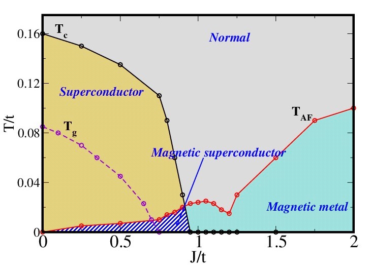
IV.2.3 Thermal effects

Since this paper is focused on the ground state we did not use the full power of the Monte Carlo method. The detailed finite temperature properties will be discussed separately, here we provide a glimpse of the finite temperature phase diagram that emerges. Beyond the ‘mean field’ effect of the diminished magnetic and superconducting order at finite temperature one expects (i) amplitude and phase fluctuations of the pairing field to suppress the gap (at low $J$) with increasing $T$, and (ii) the gap suppression effect to be accelerated by the magnetic disorder which would lead to strong spin flip scattering. These effects require a treatment well beyond mean field theory and our Boltzmann sampling of thermal configurations $\{\Delta_{i},{\bf S}_{i}\}$ accomplishes that. The thermally generated disorder feeds back into the electrons to modify spectral properties.

The superconducting $T_{c}$ falls quickly for $J>0.5t$ and goes to zero at $J_{c}\sim t$, while the low $J$ gap in the DOS closes at a scale $T_{g}$ that collapses at $J\sim 0.7t$. We note that there cannot be a finite $T_{AF}$ in a 2D ${\cal O}(3)$ invariant spin system, although the magnetic correlation length grows exponentially as $T$ is lowered below the indicated $T_{AF}$.

The data shown are at $U=4t$ where even calculations on $16\times 16$ lattices are reliable. We are working on lower $U$, which is physically more relevant, and will report the thermal properties soon.

V Conclusions

We have studied the interplay of superconductivity and magnetism in a two dimensional model involving an attractive Hubbard interaction and a Kondo like coupling to local moments. The ground state phase diagram is mapped out in terms of the attractive interaction, magnetic coupling, and electron filling. Over a range of magnetic coupling we observe a ‘gapless’ superconducting state existing generally with non-collinear magnetic order. For Neel order, superconductivity can coexist with magnetism but we do not observe a gapless phase for the bandstructure we have chosen. We identify the origin of the gapless behavior in the participation of magnetic Bloch states in the pairing process. The combination of pairing and magnetic ‘scattering’ leads to an effective ‘8 band’ dispersion, with some bands crossing the Fermi level at sufficiently large magnetic coupling. An approximate Green’s function analysis provides insight on these new bands.

The Monte Carlo technique used here in a limited way also captures the thermal physics of the problem on fairly large lattices. We have used it to map out the thermal phase diagram, determining the $T_{c}$ and $T_{AF}$ scales, presented here, and also the evolution of the spectral features across the ordering transitions. Results on this will be presented separately. The approach here generalizes naturally to the problem of $d$-wave superconductivity coexisting with magnetic order, as in some heavy fermions and ferropnictides. We are exploring these.

We acknowledge use of the High Performance Computing facility at HRI and thank Nyayabanta Swain and Sauri Bhattacharyya for comments.

VI Appendix: approximate dispersion in the gapless phase

At small $\Delta_{0}/J$, in the gapless phase, we can write explicit dispersions for the six bands that emerge from the Green’s function scheme. This involves solving for the three poles of the Green’s function, for each spin projection, at $\Delta_{0}=0$, and then calculating the small $\Delta_{0}$ corrections. In this spirit, the three poles of the up spin Green’s function at $\Delta_{0}=0$ are:

$$E_{1}^{0}({\bf k}) = E^{+}({\bf k})$$ (16)

$$E_{2}^{0}({\bf k}) = E^{-}({\bf k})$$

$$E_{3}^{0}({\bf k}) = -\epsilon({\bf k})$$

where,

$$E^{\pm}({\bf k}) = {{(\epsilon_{\bf k}+\epsilon_{\bf k+Q})\pm\sqrt{(\epsilon_{\bf k}-\epsilon_{\bf k+Q})^{2}+4J^{2}S^{2}}}\over 2}$$

The pole at $E^{0}_{3}({\bf k})=-\epsilon({\bf k})$ has residue zero (since it is artificial and cancels with a zero of the Green’s function). At $\Delta_{0}\neq 0$, however, all the poles have non zero residues, and the shifted poles are defined by $E_{\alpha}({\bf k})=E^{0}_{\alpha}({\bf k})+\eta_{\alpha}({\bf k})$, where:

$$\eta_{1}({\bf k}) = \frac{\Delta_{0}^{2}(E^{+}(\bf k)-\epsilon({\bf k+Q}))}{[(E^{+}({\bf k})-E^{-}({\bf k}))(E^{+}({\bf k})+\epsilon({\bf k}))-\Delta_{0}^{2}]}$$

$$\eta_{2}({\bf k}) = \frac{\Delta_{0}^{2}(E^{-}({\bf k})-\epsilon({\bf k+Q}))}{[(E^{-}({\bf k})-E^{+}({\bf k}))(E^{-}({\bf k})+\epsilon({\bf k}))-\Delta_{0}^{2}]}$$

$$\eta_{3}({\bf k}) = \frac{-\Delta_{0}^{2}(\epsilon({\bf k})+\epsilon({\bf k+Q}))}{[(\epsilon({\bf k})+E^{-}({\bf k}))(\epsilon({\bf k})+E^{+}({\bf k}))-\Delta_{0}^{2}]}$$ (18)

The above corrections correspond to the poles of $G_{\uparrow\uparrow}({\bf k},i\omega_{n})$. Similarly, corrections corresponding to the poles of $G_{\downarrow\downarrow}({\bf k},i\omega_{n})$ can also be determined. Together with Eqn.(5) they give corrections to the six poles for the total $G({\bf k},i\omega_{n})$.

References

- (1) V. L. Ginzburg, Sov. Phys. JETP 4, 153 (1957).
- (2) M. L. Kulic and A. I. Buzdin In: Superconductivity, Eds: K. H. Bennemann and J. B. Ketterson, (Springer), (2008), Chap. 4, p. 163.
- (3) A. Abrikosov and L. P. Gorkov, Sov. Phys. JETP 12, 1243 (1961).
- (4) W. Baltensperger and S. Strassler, Z. Phys. B 1, 20 (1963).
- (5) M. B. Maple and O. Fisher, Superconductivity in ternary compounds II, Superconductivity and Magnetism (Berlin: Springer) (1982).
- (6) O. Fisher and M. B. Maple, Superconductivity in Ternary Compounds I, Structural, Electronic and Lattice Properties (Berlin: Springer) (1982).
- (7) P. Fulde, J. Keller, In: Superconductivity and Magnetism, Eds. M.B. Maple and O. Fischer (Springer, Berlin, 1982) Chap. 9, p. 249
- (8) J. W. Lynn, P. C. Canfield, G. Hilscher, K-H. Muller and V. N. Narozhnyi, Progress in borocarbide research, Rare Earth Transition Metal Borocarbides (Nitrides): Superconducting, Magnetic and Normal State Properties ed K-H M ̵̈uller and V N Narozhnyi (Dordrecht: Kluwer) (2001).
- (9) J. W. Lynn, J. A. Gotaas, R. W. Erwin, R. A. Ferell, J. K. Bhattacharjee, R. N. Shelton and P. Klavins, Phys. Rev. Lett. 52, 133 (1984).
- (10) W. Thomlinson, G. Shirane, J. W. Lynn and D. E. Moncton, Neutron scattering studies of magnetic order in ternary superconductors, in Superconductivity in Ternary Compounds II, Superconductivity and Magnetism ed M B Maple and ø Fischer (Berlin: Springer) (1982).
- (11) G. Zwicknagl and P. Fulde, Z. Phys. B: Condens. Matter 43, 23 (1981).
- (12) P. A. Lee, N. Nagaosa and X-G. Wen, Rev. Mod. Phys. 78, 17 (2006).
- (13) G. R. Stewart, Rev. Mod. Phys. 83, 1589 (2011).
- (14) D. C. Johnson, Adv. Phys. 59, 803 (2010).
- (15) F-C. Hsu, J-Y. Luo, K-W. Yeh,T-K. Chen, T-W. Huang, P. M. Wu, Y-C. Lee, Y-L. Huang, Y-Y. Chu, D-C. Yan and M-K. Wu, Proc. Nat. Acad. Sci. USA 105, 14262 (2008).
- (16) M. H. Fang, H. M. Pham, B. Qian, T. J. Liu, E. K. Vehstedt, Y. Liu, L. Spinu and Z. Q. Mao, Phys. Rev. B 78, 224503 (2008).
- (17) J. Guo, S. Jin, G. Wang, S. Wang, K. Zhu, T. Zhou, M. He and X. Chen, Phys. Rev. B 82, 180520 (2010).
- (18) M-H. Fang, H-D. Wang, C-H. Dong, Z-J. Li, C-M. Feng, J. Chen and H. Q. Yuan, Eur. Phys. Lett. 94, 27009 (2011).
- (19) P. Dai, J. Hu and E. Dagotto, Nat. Phys. 8, 709 (2012).
- (20) E. Wiesenmayer, H. Luetkens, G. Pascua, R. Khasanov, A. Amato, H. Potts, B. Banusch, H-H. Klauss and D. Johrendt, Phys. Rev. Lett. 107, 237001 (2011).
- (21) S. S. Saxena, P. Agarwal, K. Ahilan, F. M. Grosche, R. K. W. Haselwimmer, M. J. Steiner, E. Pugh, I. R. Walker, S. R. Julian, P. Monthoux, G. G. Lonzarich, A. Huxley, I. Sheikin, D. Braithwaite and J. Flouquet, Nature (London) 406, 587 (2000).
- (22) D. J. Scalapino, Rev. Mod. Phys. 84, 1383 (2012).
- (23) M. Nicklas, O. Stockert, T. Park, K. Habicht, K. Kiefer, L. D. Pham, J. D. Thompson, Z. Fisk and F. Steglich, Phys. Rev. B 76, 052401 (2007).
- (24) L. D. Pham, T. Park, S. Maquilon, J. D. Thompson and Z. Fisk, Phys. Rev. Lett. 97, 056404 (2006).
- (25) C. Pfleiderer, Rev. Mod. Phys. 81, 1551 (2009).
- (26) K-H Muller and V N Narozhnyi, Rep. Prog. Phys. 64, 943-1008 (2001).
- (27) M. B. Maple, Physica B 215, 110 (1995).
- (28) J. W. Lynn, S. Skanthakumar, Q. Huang, S. K. Sinha, Z. Hossain, L. C. Gupta, R. Nagarajan and C. Godart, Phys. Rev. B 55, 6584 (1997).
- (29) L. C. Gupta, Phil. Mag. 77, 717 (1998).
- (30) H. Michor, M. El-Hagary, R. Hauser, E. Bauer and G. Hilscher, Physica B, 259, 604 (1999).
- (31) H. F. Braun, Superconductivity and magnetism in ruthenocuprates and borocarbides, in Rare Earth Transition Metal Borocarbides (Nitrides): Superconducting, Magnetic and Normal State Properties ed K-H Muller and V N Narozhnyi (Dordrecht: Kluwer) (2001).
- (32) M. Schneider, G. Fuchs, K.-H. Muller, K. Nenkov, G. Behr, D. Souptel and S.-L. Drechsler, Phys. Rev. B 80, 224522 (2009).
- (33) T. Baba, T. Yokoya, S. Tsuda, T. Kiss, T. Shimojima, K. Ishizaka, H. Takeya, K. Hirata, T. Watanabe, M. Nohara, H. Takagi, N. Nakai, K. Machida, T. Togashi, S. Watanabe, X.-Y. Wang, C. T. Chen and S. Shin, Phys. Rev. Lett. 100, 017003 (2008).
- (34) L. F. Rybaltchenko, A. G. M. Jansen, P. Wyder, L. V. Tjutrina, P. C. Canfield, C. V. Tomy, D. McK. Paul, Physica C 319, 189 (1999).
- (35) Yu. G. Naidyuk, O. E. Kvitnitskaya, L. V. Tiutrina, I. K. Yanson, G. Behr, G. Fuchs, S.-L. Drechsler, K. Nenkov and L. Schultz, Phys. Rev. B 84, 094516 (2011).
- (36) E. I. Blount and C. M. Varma, Phys. Rev. Lett. 42, 1079 (1979).
- (37) H. S. Greenside, E. I. Blount and C. M. Varma, Phys. Rev. Lett. 46, 49 (1980).
- (38) C. G. Kuper, M. Revzen and A. Ron, Phys. Rev. Lett. 44, 1545 (1980).
- (39) K. Machida, K. Nokura and T. Matsubara, Phys. Rev. B 22, 2307 (1980).
- (40) M. J. Nass, K. Levin and G. S. Grest, Phys. Rev. B 25, 4541 (1982).
- (41) M. J. Nass, K. Levin and G. S. Grest, Phys. Rev. Lett. 46, 614 (1981); C. Ro and K. Levin, Phys. Rev. B 29, 6155 (1984).
- (42) Y. Suzumura and A. D. S. Nagi, Sol. State. Commn. 40, 651 (1981).
- (43) O. Sakai, M. Tachiki, T. Koyama, H. Matsumoto and H. Umezawa, Phys. Rev. B 24, 3830 (1981).
- (44) E. W. Fenton, Sol. State Commn. 65, 343 (1988).
- (45) H. Kontani, Phys. Rev. B 70, 054507 (2004).
- (46) L. N. Bulaevskii, A. I. Buzdin, M. L. Kulic and S. V. Panjukov, Adv. Phys. 34, 175 (1985).
- (47) L. N. Bulaevskii, A. I. Buzdin and M. L. Kulic, Phys. Rev. B 34, 4928 (1986); L. N. Bulaevskii, A. I. Buzdin, M. L. Kulic and S. V. Panyukov, Phys. Rev. B 28, 1370 (1983); M. L. Kulic, Phys. Rep. 338, 1 (2000); M. L. Kulic and Dolgov, Phys. Stat. Sol. B 242, 151 (2005); A. I. Buzdin, Rev. Mod. Phys. 77, 935 (2005).
- (48) L. N. Bulaevskii, A. I. Buzdin and M. L. Kulic, Phys. Lett. 85A, 161 (1981)
- (49) D. Pines, Physica B 163, 78 (1990).
- (50) A. V. Chubukov, Eur. Phys. Lett. 44, 655 (1998).
- (51) A. Abanov, A. V. Chubukov and J. Schmalian, Adv. Phys. 52, 119 (2003).
- (52) R. H. Mckenzie, Science 278, 820 (1997).
- (53) H. Kino and H. Fukuyama, J. Phys. Soc. Japan 65, 2158 (1996).
- (54) J. Schmalian, Phys. Rev. Lett. 81, 4232 (1998).
- (55) H. Kino and H. Kontani, J. Phys. Soc. Japan 68, 1481 (1999).
- (56) M. Inada, T. Sasaki, T. Nishizaki, N. Kobayashi, S. Yamada and T. Fukase, J. Low. Temp. Phys. 117, 1423 (1999).
- (57) N. I. Karchev, K. B. Blagoev, K. S. Bedell and P. B. Littlewood, Phys. Rev. Lett. 86, 846 (2001).
- (58) J. A. Hertz, K. Levin and M. T. Beal-Monod, Sol. State Commn. 18, 803 (1976).
- (59) M. T. Beal Monod, C. Bourbonnais and V. J. Emery, Phys. Rev. B 34, 7716 (1986).
- (60) D. J. Scalapino E. Loh. Jr. and J. E. Hirsch, Phys. Rev. B 35, 6694 (1987).
- (61) K. Miyake, S. Schmitt-Rink and C.M. Varma, Phys. Rev. B 34, 6554 (1986).
- (62) J. Jensen and P. Hedegard, Phys. Rev. B 76, 094504 (2007).
- (63) P. R. Bertussi, A. L. Malvezzi, T. Paiva and R. R. dos Santos, Phys. Rev. B, 79, 220513 (2009).
- (64) O Bodensiek, T Pruschke and R Zitko, J. Phys. Conf. Series 200, 012162 (2009).
- (65) A. Amici, P. Thalmeier and P. Fulde, Phys. Rev. Lett. 84, 1800 (2000).
- (66) J. Jensen, Phys. Rev. B 65, 140514 (2002).
- (67) K. Maki, H. Won and S. Haas, Phys. Rev. B 69, 012502 (2004).
- (68) S Lee, H. Won, H. Y. Chen, Q. Yuan, K. Maki and P. Thalmeier, J. Mag. Mag Mat. 272, E145 (2004).
- (69) A. O. Shorikov, V. I. Anisimov and M. Sigrist, J. Phys. Cond. Mat. 18, 5973 (2006).
- (70) K. Maki, P. Thalmeier and H. Won, Physica C 408-410, 681 (2004).
- (71) P. W. Anderson and H. Suhl, Phys. Rev. 116, 898 (1959).
- (72) G. Sarma, J. Phys. Chem. Solids, 24, 1029 (1963); P. Fulde and R. A. Ferrell, Phys. Rev. 135, A550 (1964); A. I. Larkin and Yu. N. Ovchinnikov, Zh. Eksp. Teor. Fiz. 47, 1136 (1964); Sov. Phys. JETP 20, 762 (1965); T. K. Koponen, T. Paananen, J.-P. Martikainen and P. Torma, Phys. Rev. Lett. 99, 120403 (2007); M. J. Wolak, B. Gremaud, R. T. Scalettar and G. G. Batrouni, Phys. Rev. A 86, 023630 (2012); Y. L. Loh and N. Trivedi, Phys. Rev. Lett. 104, 165302 (2010).
- (73) M. Karmakar and P. Majumdar, arXiv:1508:00393v1, and the references therein.
- (74) M. Divis, K. Schwartz, P. Blaha, G. Hilscher, H. Michor and S. Khmelevskyi, Phys. Rev. B 62, 6774 (2000).
- (75) P. Martínez-Samper, H. Suderow, S. Vieira, J. P. Brison, N. Luchier, P. Lejay and P. C. Canfield, Phys. Rev. B 67, 014526 (2003).
- (76) K. Izawa, K. Kamata, Y. Nakajima, Y. Matsuda, T. Watanabe, M. Nohara, H. Takagi, P. Thalmeier and K. Maki, Phys. Rev. Lett. 89, 137006 (2002).
- (77) T. Watanabe, M. Nohara, T. Hanaguri and H. Takagi, Phys. Rev. Lett. 92, 147002 (2004).
- (78) T. Baba, T. Yokoya, S. Tsuda, T. Watanabe, M. Nohara, H. Takagi, T. Oguchi and S. Shin, Phys. Rev. B 81, 180509(R) (2010).
- (79) N. L. Bobrov, V. N. Chernobay, Yu. G. Naidyuk, L. V. Tyutrina, D. G. Naugle, K. D. D. Rathnayaka,S. L. Budko, P. C. Canfield and I. K. Yanson, Eur. Phys. Lett. 83, 37003 (2008).
- (80) I.K Yanson, N.L Bobrov, C.V Tomy and D.McK Paul, Physica C 334, 33 (2000).