Incremental Spectral Sparsification for Large-Scale Graph-Based Semi-Supervised Learning

Abstract

While the harmonic function solution performs well in many semi-supervised learning (SSL) tasks, it is known to scale poorly with the number of samples. Recent successful and scalable methods, such as the eigenfunction method [11] focus on efficiently approximating the whole spectrum of the graph Laplacian constructed from the data. This is in contrast to various subsampling and quantization methods proposed in the past, which may fail in preserving the graph spectra. However, the impact of the approximation of the spectrum on the final generalization error is either unknown [11], or requires strong assumptions on the data [15]. In this paper, we introduce Sparse-HFS, an efficient edge-sparsification algorithm for SSL. By constructing an edge-sparse and spectrally similar graph, we are able to leverage the approximation guarantees of spectral sparsification methods to bound the generalization error of Sparse-HFS. As a result, we obtain a theoretically-grounded approximation scheme for graph-based SSL that also empirically matches the performance of known large-scale methods.

1 Introduction

In many classification and regression tasks, obtaining labels for large datasets is expensive. When the number of labeled samples is too small, traditional supervised learning algorithms fail in learning accurate predictors. Semi-supervised learning (SSL) [7, 29] effectively deals with this problem by integrating the labeled samples with an additional set of unlabeled samples, which are abundant and readily available in many applications (e.g., set of images collected on web sites [11]). The intuition behind SSL is that unlabeled data may reveal the underlying structure of the problem (e.g., a manifold) that could be exploited to compensate for the limited number of labels and improve the prediction accuracy. Among different SSL settings, in this paper we focus on the case where data are embedded in a graph. The graph is expected to effectively represent the geometry of data and graph-based SSL [30, 3, 25] methods leverage the intuition that nodes that are similar according to the graph are more likely to be labeled similarly. A popular approach is the harmonic function solution (HFS) [30, 2, 11], whose objective is to find a solution where each node’s value is the weighted average of its neighbors. Computing the HFS solution requires solving a Laplacian regularized least-squares problem. While the resulting solution is both empirically effective [11] and enjoys strong performance guarantees [3, 9], solving exactly the least-squares problem on a graph with $n$ nodes amounts to $\mathcal{O}(n^{3})$ time and $\mathcal{O}(n^{2})$ space complexity. Using a general iterative solver on a graph with $m$ edges to obtain a comparable solution requires only $\mathcal{O}(mn)$ time and $\mathcal{O}(m)$ space, but this is still practically unfeasible in many applications of interest. In fact, many graphs have naturally a large number of edges, so that even if the $n$ nodes could fit in memory, storing $m$ edges largely exceeds the memory capacity. For instance, Facebook’s graph of relationships [8] counts about $n=1.39e9$ users connected by a trillion ($m=1e12$) edges. While $n$ is still in the order of the memory capacity, the edges cannot be stored in a single computer. A similar issue is faced when the graph is built starting from a dataset, for instance using a $k$-nn graph. In this case $m=kn$ edges are created, and sometimes a large $k$ is necessary to obtain good performance [23], or artificially adding neighbours can improve the stability of the method [13]. In such problems, a direct application of HFS is not possible and thus some form of approximation or graph sketching is required. A straightforward approach is to distribute the graph over multiple machines in a cluster and resort to an iterative solver for the solution of the least-squares problem [8]. Distributed algorithms require infrastructure and careful engineering in order to deal with communication issues [6]. But even assuming that these problems are satisfactorily dealt with, all known iterative solvers that have provably fast convergence do not have known distributed implementations, as they assume random, constant time access to all the edges in the graph. Thus one would have to resort to distributed implementations of simpler but much slower methods, in effect trading-off space for a significant reduction in overall efficiency.

More principled methods try to address the memory bottleneck by directly manipulating the structure of the graph to reduce its size. These include subsampling the nodes of the original graph, quantization, approaches related to manifold learning, and various approximation strategies. The most straightforward way to reduce the complexity in graph-based method is to subsample the nodes to create a smaller, backbone graph of representative vertices, or landmarks [26]. Nyström sampling methods [20] randomly select $s$ nodes from the original graph and compute $q$ eigenvectors of the smaller graph, which can be later used to solve the HFS regularized problem. It can be shown [20] that the reconstructed Laplacian is accurate in $\ell_{2}$-norm and thus only its largest eigenvalue is preserved. Unfortunately, the HFS solution does not depend only on the largest eigenvalues, both because the largest eigenvectors are the ones most penalized by HFS’s regularizer ([3]) and because theoretical analysis shows that preserving the smallest eigenvalue is important for generalization bounds ([2]). As a result, subsampling methods can completely fail when the sampled nodes compromise the spectral structure of the graph [11]. Although alternative techniques have been developed over years (see e.g., [14, 28, 31, 12, 27, 22]), this drawback is common to all backbone graph methods. Motivated by this observation, other approaches focus on computing a more accurate approximation of the spectrum of the Laplacian. Fergus et al. [11] build on the observation that when the number of unlabeled samples$n$ tends to infinity, the eigenvectors of the Laplacian tend to the eigenfunctions of the sampling distribution $\mathcal{P}$. Thus instead of approximating eigenvectors in $\mathbb{R}^{n}$, they first compute empirical eigenfunctions of the estimated sampling distribution (defined on the $d$-dimensional feature space) obtained by assuming that $\mathcal{P}$ is factorized and by using a histogram estimation over $b$ bins over each dimension separately. While the method scales to the order of million nodes, it still requires $d$ and $b$ to be small to be efficient. Furthermore, no theoretical analysis is available, and the method may return poor approximations whenever the sampling distribution is not factorized. Motivated by the empirical success of [11], Ji et al. [15] proposed a similar algorithm, Simple-HFS, for which they provide theoretical guarantees. However, in order to prove bounds on the generalization error, they need to assume several strong and hard to verify assumptions, such as a sufficiently large eigengap. On the contrary, the guarantees for our method work for any graph.

Our contribution

In this paper, we focus on reducing the space complexity of graph-based SSL while matching the smallest possible computational complexity of $\Omega(m)$ up to logarithmic factors and providing strong guarantees about the quality of the solution. In particular, we introduce a novel approach which employs efficient spectral graph sparsification techniques [17] to incrementally process the original graph. This method, coupled with dedicated solvers for symmetric diagonally dominant (SDD) systems [19], allows to find an approximate HFS solution without storing the whole graph in memory and to control the computational complexity as $n$ grows. In fact, we show that our proposed method, called Sparse-HFS, requires only fixed $\mathcal{O}(n\log^{2}(n))$ space to run, and allows to compute solutions to large HFS problems in memory. For example, in the experimental section we show that the sparsifier can achieve an accuracy comparable to the full graph, using one order of magnitude less edges. With a careful choice of the frequency of resparsification, the proposed method does not increase significantly the running time. Given a minimum amortized cost of $\Omega(1)$ per edge, necessary to examine each edge at least once, our algorithm only increases this cost to $\mathcal{O}(\log^{3}(n))$. Furthermore, using the approximation properties of spectral sparsifiers and results from algorithmic stability theory [5, 9] we provide theoretical guarantees for the generalization error for Sparse-HFS, showing that the performance is asymptotically the same as the exact solution of HFS. Finally, we report empirical results on both synthetic and real data showing that Sparse-HFS is competitive with subsampling and the EigFun method in [11].

2 Graph-Based Semi-Supervised Learning

Notation. We denote with lowercase letter $a$ a scalar, with bold lowercase letter $\mathbf{a}$ a vector and with uppercase letter $A$ a matrix. We consider the problem of regression in the semi-supervised setting, where a large set of $n$ points $\mathcal{X}=(\mathbf{x}_{1},\ldots,\mathbf{x}_{n})\subset\mathbb{R}^{d}$ is drawn from a distribution $\mathcal{P}$ and labels $\{y_{i}\}_{i=1}^{l}$ are provided only for a small (random) subset $\mathcal{S}\subset\mathcal{X}$ of $l$ points. Graph-based SSL builds on the observation that $\mathcal{P}$ is often far from being uniform and it may display a specific structure that could be exploited to “propagate” the labels to similar unlabeled points. Building on this intuition, graph-based SSL algorithms consider the case when the points in $\mathcal{X}$ are embedded into an undirected weighted graph $\mathcal{G}=(\mathcal{X},\mathcal{E})$ with $|\mathcal{E}|=m$ edges. Associated with each edge $e_{i,j}\in\mathcal{E}$ there is a weight $a_{e_{i,j}}$ measuring the “distance” between $\mathbf{x}_{i}$ and$\mathbf{x}_{j}$. A graph-based SSL algorithm receives as input $\mathcal{G}$ and the labels of the nodes in $\mathcal{S}$ and it returns a function $\mathbf{f}:\mathcal{X}\rightarrow\mathbb{R}$ that predicts the label for all nodes in $\mathcal{X}$. The objective is to minimize the prediction error over the set $\mathcal{T}$ of $u=n-l$ unlabeled nodes. In the following we denote by $\mathbf{y}\in\mathbb{R}^{n}$ the full vector of labels.

Stable-HFS. HFS directly exploits the structure embedded in $\mathcal{G}$ to learn functions that are smooth over the graph, thus predicting similar labels for similar nodes. Given the weighted adjacency matrix $A_{\mathcal{G}}$ and the degree matrix $D_{\mathcal{G}}$, the Laplacian of $\mathcal{G}$ is defined as $L_{\mathcal{G}}=D_{\mathcal{G}}-A_{\mathcal{G}}$. The Laplacian $L_{\mathcal{G}}$ is semi-definite positive (SDP) with $\operatorname*{Ker}(L_{\mathcal{G}})=\mathbf{1}$. Furthermore, we assume that $\mathcal{G}$ is connected and thus has only one eigenvalue at $0$. Let $L_{\mathcal{G}}^{+}$ be the pseudoinverse of $L_{\mathcal{G}}$, and $L_{\mathcal{G}}^{-1/2}=(L_{\mathcal{G}}^{+})^{1/2}$. The HFS method [30] can be formulated as the Laplacian-regularized least-squares problem

$$\widehat{\mathbf{f}} =\operatorname*{arg\,min}_{\mathbf{f}\in\mathbb{R}^{n}}\tfrac{1}{l}(\mathbf{f}-\mathbf{y})^{\mathsf{T}}I_{\mathcal{S}}(\mathbf{f}-\mathbf{y})+\gamma\mathbf{f}^{\mathsf{T}}L_{\mathcal{G}}\mathbf{f},$$ (1)

where $I_{\mathcal{S}}\in\mathbb{R}^{n\times n}$ is the identity matrix with zeros corresponding to the nodes not in $\mathcal{S}$ and $\gamma$ is a regularization parameter. The solution can be computed in closed form as $\widehat{\mathbf{f}}=(\gamma lL_{\mathcal{G}}+I_{\mathcal{S}})^{+}\mathbf{y}_{\mathcal{S}}$, where $\mathbf{y}_{\mathcal{S}}=I_{\mathcal{S}}\mathbf{y}\in\mathbb{R}^{n}$. The singularity of the Laplacian may lead to unstable behavior with drastically different results for small perturbations to the dataset. For this reason, we focus on the Stable-HFS algorithm proposed in [2] where an additional regularization term is introduced to restrict the space of admissible hypotheses to the space $\mathcal{F}=\left\{\mathbf{f}:\langle\mathbf{f},\mathbf{1}\rangle=0\right\}$ of functions orthogonal to null space of $L_{\mathcal{G}}$ (i.e., centered functions). This restriction can be easily enforced by introducing an additional regularization term $\frac{\mu}{l}\mathbf{f}^{\top}\mathbf{1}$ in Eq. 1. As shown in [2], in order to guarantee that the resulting $\widehat{\mathbf{f}}$ actually belongs to $\mathcal{F}$, it is sufficient to set the regularization parameter to $\mu=((\gamma lL_{\mathcal{G}}+I_{\mathcal{S}})^{+}\mathbf{y}_{S})^{\mathsf{T}}\mathbf{1}/((\gamma lL_{\mathcal{G}}+I_{\mathcal{S}})^{+}\mathbf{1})^{\mathsf{T}}\mathbf{1}$, and compute the solution as $\widehat{\mathbf{f}}=(\gamma lL_{\mathcal{G}}+I_{\mathcal{S}})^{+}(\mathbf{y}_{\mathcal{S}}-\mu\mathbf{1})$. Furthermore, it can be shown that if we center the vector of labels $\widetilde{\mathbf{y}}_{\mathcal{S}}=\mathbf{y}_{\mathcal{S}}-\overline{\mathbf{y}}_{\mathcal{S}}$, with $\overline{\mathbf{y}}=\frac{1}{l}\mathbf{y}_{\mathcal{S}}^{\mathsf{T}}\mathbf{1}$, then the solution of Stable-HFS can be rewritten as $\widehat{\mathbf{f}}=(\gamma lL_{\mathcal{G}}+I_{\mathcal{S}})^{+}(\widetilde{\mathbf{y}}_{\mathcal{S}}-\mu\mathbf{1})=\big{(}P_{\mathcal{F}}(\gamma lL_{\mathcal{G}}+I_{\mathcal{S}})\big{)}^{+}\widetilde{\mathbf{y}}_{\mathcal{S}}$, where $P_{\mathcal{F}}=L_{\mathcal{G}}L_{\mathcal{G}}^{+}$ is the projection matrix on the $n-1$ dimensional space $\mathcal{F}$. Indeed, since the Laplacian of any graph $\mathcal{G}$ has a null space equal to the one vector $\mathbf{1}$, then $P_{\mathcal{F}}$ is invariant w.r.t. the specific graph $\mathcal{G}$ used to defined it. While Stable-HFS is more stable and thus more suited for theoretical analysis, its time and space requirements remain $\mathcal{O}(mn)$ and $\mathcal{O}(m)$, and cannot be applied to graph with a large number of edges.

3 Spectral Sparsification for Graph-Based SSL

0:  Graph $\mathcal{G}=(\mathcal{X},\mathcal{E})$, labels $\mathbf{y}_{\mathcal{S}}$, accuracy $\varepsilon$ 0:  Solution $\widehat{\mathbf{f}}$, sparsified graph $\mathcal{H}$   Let $\alpha=1/(1-\varepsilon)$ and $N=\alpha^{2}n\log^{2}(n)/\varepsilon^{2}$   Partition $\mathcal{E}$ in $\tau=\lceil m/N\rceil$ blocks $\Delta_{1},\ldots,\Delta_{\tau}$   Initialize $\mathcal{H}=\emptyset$   for $t=1,\ldots,\tau$ do     Load $\Delta_{t}$ in memory     Compute $\mathcal{H}_{t}=\textsc{sparsify}(\mathcal{H}_{t-1},\Delta_{t},N,\alpha)$   end for   Center the labels $\widetilde{\mathbf{y}}_{\mathcal{S}}$   Compute $\widetilde{\mathbf{f}}$ with Stable-HFS with $\widetilde{\mathbf{y}}_{\mathcal{S}}$ using a suitable SDD solver

Figure 1: Sparse-HFS

In this section we introduce a novel variant of HFS, called Sparse-HFS, where spectral graph sparsification techniques are integrated into Stable-HFS, drastically reducing the time and memory requirements without compromising the resulting accuracy.

Spectral sparsification. A graph sparsifier receives as input a graph $\mathcal{G}$ and it returns a graph $\mathcal{H}$ on the same set of nodes $\mathcal{X}$ but with much fewer edges. Among different techniques [1], spectral sparsification methods provide the stronger guarantees on the accuracy of the resulting graph.

Definition 1.

A $1\pm\varepsilon$ spectral sparsifier of $\mathcal{G}$ is a graph $\mathcal{H}\subseteq\mathcal{G}$ such that for all $\mathbf{x}\in\mathbb{R}^{n}$

$$(1-\varepsilon)\mathbf{x}^{\mathsf{T}}L_{\mathcal{G}}\mathbf{x}\leq\mathbf{x}^{\mathsf{T}}L_{\mathcal{H}}\mathbf{x}\leq(1+\varepsilon)\mathbf{x}^{\mathsf{T}}L_{\mathcal{G}}\mathbf{x}.$$

The key idea [24] is that to construct a sparse graph $\mathcal{H}$, it is sufficient to randomly select $m^{\prime}=\mathcal{O}(n\log(n)/\varepsilon^{2})$ edges from $\mathcal{G}$ with a probability proportional to their effective resistance and add them to the new graph with suitable weights. While storing the sparsified graph requires only $\mathcal{O}(m^{\prime})$ space, it still suffers from major limitations: (i) the naive computation of the effective resistances needs $\mathcal{O}(mn\log(n))$ time, (ii) it requires $\mathcal{O}(m)$ space to store the initial graph $\mathcal{G}$, and (iii) computing the HFS solution on $\mathcal{H}$ in a naive way still has a cost of $\mathcal{O}(m^{\prime}n)$. For this reason, we employ more sophisticated solutions and integrate the recent spectral sparsification technique for the semi-streaming setting in [17] and the efficient solver for SDD systems in [19]. The resulting algorithm is illustrated in Fig. 1.

0:  A sparsifier $\mathcal{H}$, block $\Delta$, number of edges $N$, effective resistance accuracy $\alpha$ 0:  A sparsifier $\mathcal{H}^{\prime}$, probabilities $\{\widetilde{p}^{\prime}_{e}:e\in\mathcal{H}^{\prime}\}$.   Compute estimates of $\widetilde{R}^{\prime}_{e}$ for any edge in $\mathcal{H}+\Delta$ such that $1/\alpha\leq\widetilde{R}^{\prime}_{e}/R^{\prime}_{e}\leq\alpha$ with an SDD solver [19]   Compute probabilities $\widetilde{p}^{\prime}_{e}=(a_{e}\widetilde{R}^{\prime}_{e})/(\alpha(n-1))$ and weights $w_{e}=a_{e}/(N\widetilde{p}^{\prime}_{e})$   For all edges $e\in\mathcal{H}$ compute $\widetilde{p}^{\prime}_{e}\leftarrow\min\{\widetilde{p}_{e},\widetilde{p}^{\prime}_{e}\}$ and initialize $\mathcal{H}^{\prime}=\emptyset$   for all edges $e\in\mathcal{H}$ do     Add edge $e$ to $\mathcal{H}^{\prime}$ with weight $w_{e}$ with prob. $\widetilde{p}^{\prime}_{e}/\widetilde{p}_{e}$   end for   for all edges $e\in\Delta$ do     for $i=1$ to $N$ do        Add edge $e$ to $\mathcal{H}^{\prime}$ with weight $w_{e}$ with prob. $\widetilde{p}^{\prime}_{e}$     end for   end for

Figure 2: Kelner-Levin Sparsification algorithm [17]

We first introduce additional notation. Given two graphs $\mathcal{G}$ and $\mathcal{G}^{\prime}$ over the same set of nodes $\mathcal{X}$, we denote by $\mathcal{G}+\mathcal{G}^{\prime}$ the graph obtained by summing the weights on the edges of $\mathcal{G}^{\prime}$ to $\mathcal{G}$. For any node $i=1,\ldots,n$, we denote with $\chi_{i}\in\mathbb{R}^{n}$ the indicator vector so that $\chi_{i}-\chi_{j}$ is the “edge” vector. The effective resistance of an edge $e_{i,j}$ in a graph $\mathcal{G}$ is equal to $R_{e_{i,j}}=(\chi_{i}-\chi_{j})^{\mathsf{T}}L_{\mathcal{G}}^{+}(\chi_{i}-\chi_{j})$. The key intuition behind our Sparse-HFS is that processing the graph incrementally allows to dramatically reduce the memory requirements and keep low time complexity at the same time. Let $\varepsilon$ be the (spectral) accuracy desired for the final sparsified graph $\mathcal{H}$, Sparse-HFS first partitions the set of edges $\mathcal{E}$ of the original graph $\mathcal{G}$ into $\tau$ blocks $(\Delta_{1},\ldots,\Delta_{\tau})$ of size $N=\alpha^{2}n\log^{2}(n)/\varepsilon^{2}$, with $\alpha=1/(1-\varepsilon)$. While the original graph with $m$ edges is too large to fit in memory, each of these blocks has a number of edges which is nearly linear in the number of nodes and can be easily managed. Sparse-HFS processes blocks over iterations. Starting with an empty graph $\mathcal{H}_{0}$, at each iteration $t$ a new block $\Delta_{t}$ is loaded and the intermediate sparsifier $\mathcal{H}_{t-1}$ is updated using the routine sparsify, which is guaranteed to return a $(1\pm\varepsilon)$-sparsifier of size $N$ for the graph $\mathcal{H}_{t-1}+\Delta_{t}$. After all the blocks are processed, a sparsifier $\mathcal{H}$ is returned and the Stable-HFS solution can be computed. Since $\mathcal{H}$ is very sparse (i.e., it only contains $N=\mathcal{O}(n\log^{2}(n))$ edges), it is now possible to use efficient solvers for linear sparse systems and drastically reduce the computational complexity of solving Stable-HFS from $\mathcal{O}(Nn)$ down to $\mathcal{O}(N\log(n))$. The routine sparsify can be implemented using different spectral sparsification techniques developed for the streaming setting, here we rely on the method proposed in [17]. The effective resistance is computed for all edges in the current sparsifier and the new block using random projections and an efficient solver for SDD systems [19]. This step takes $\mathcal{O}(N\log n)$ time and it returns $\alpha$-accurate estimates $\widetilde{R}^{\prime}_{e}$ of the effective resistance for the $2N$ nodes in $\mathcal{H}_{t-1}$ and $\Delta_{t}$. If $\alpha=1/(1-\varepsilon)$ and the input graph $\mathcal{H}_{t-1}$ is a $(1\pm\varepsilon)$-sparsifier, then sampling $N$ edges proportionally to $\widetilde{R}^{\prime}_{e}$ is guaranteed to generate a $(1\pm\varepsilon)$-sparsifier for the full graph $\mathcal{G}_{t}=\sum_{s=1}^{t}\Delta_{s}$ up to iteration $t$. More details on this process are provided in Fig. 2 and in [17]. The resulting process has a space complexity $\mathcal{O}(N)$ and a time complexity that never exceeds $\mathcal{O}(N\log(n))$ in sparsifying each block and computing the final solution (see next section for more precise statements on time and space complexity).

4 Theoretical Analysis

We first report the time and space complexity of Sparse-HFS. This result follows from the properties of the sparsifier in [17] and the SDD solver in [19] and thus we do not report its proof.

Lemma 1.

Let $\varepsilon>0$ be the desired accuracy and $\delta>0$ the probability of failure. For any connected graph $\mathcal{G}=(\mathcal{X},\mathcal{E})$ with $n$ nodes, $m$ edges, eigenvalues $0=\lambda_{1}(\mathcal{G})<\lambda_{2}(\mathcal{G})\leq\ldots\leq\lambda_{n}(\mathcal{G})$, and any partitioning of $\mathcal{E}$ into $\tau$ blocks, Sparse-HFS returns a graph $\mathcal{H}$ such that for any $i=1,\ldots,n$

$$(1-\varepsilon)\lambda_{i}(\mathcal{G})\leq\lambda_{i}(\mathcal{H})\leq(1+\varepsilon)\lambda_{i}(\mathcal{G}),$$ (2)

with prob. $1-\delta$ (w.r.t. the random estimation of the effective resistance and the sampling of edges in the sparsify routine). Furthermore, let $N=\alpha^{2}n\log^{2}(n)/\varepsilon^{2}$ for $\alpha=1/(1-\varepsilon)$ and $\tau=m/N$, then with prob. $1-\delta$ Sparse-HFS has an amortized time per edge of $\mathcal{O}(\log^{3}(n))$ and it requires $\mathcal{O}(N)$ memory.

The previous lemma shows the dramatic improvement of Sparse-HFS w.r.t. Stable-HFS in terms of both time and space complexity. In fact, while solving Stable-HFS in a naive way can take up to $\mathcal{O}(m)$ space and $\mathcal{O}(mn)$ time, Sparse-HFS drops these requirements down to $\mathcal{O}(n\log^{2}(n)/\varepsilon^{2})$ space and $\mathcal{O}(m\log^{3}(n))$ time, which allows scaling Stable-HFS to graphs orders of magnitude bigger. These improvements have only a limited impact on the spectrum of $\mathcal{G}$ and all its eigenvalues are approximated up to a $(1\pm\varepsilon)$ factor. Moreover, all of the sparsification guarantees hold w.h.p. for any graph, regardless of how it is generated, its original spectra, and more importantly regardless of the exact order in which the edges are assigned to the blocks. Finally, we notice that the choice of the number of blocks as $m/N$ is crucial to guarantee a logarithmic amortized time, since each iteration takes $\mathcal{O}(N\log^{3}(n))$ time. As discussed in Sect. 6, this property allows to directly apply Sparse-HFS in online learning settings where edges arrive in a stream and intermediate solutions have to be computed incrementally. In the following, we show that, unlike other heuristics, the space complexity improvements obtained with sparsification come with guarantees and do not degrade the actual learning performance of HFS. The analysis of SSL algorithms is built around the algorithm stability theory [5], which is extensively used to analyse transductive learning algorithms [10, 9]. We first remind the definition of algorithmic stability.

Definition 2.

Let $\mathcal{L}$ be a transductive learning algorithm. We denote by $\mathbf{f}$ and $\mathbf{f}^{\prime}$ the functions obtained by running $\mathcal{L}$ on datasets $\mathcal{X}=(\mathcal{S},\mathcal{T})$ and $\mathcal{X}=(\mathcal{S}^{\prime},\mathcal{T}^{\prime})$ respectively. $\mathcal{L}$ is uniformly $\beta$-stable w.r.t. the squared loss if there exists $\beta\geq 0$ such that for any two partitions $(\mathcal{S},\mathcal{T})$ and $(\mathcal{S}^{\prime},\mathcal{T}^{\prime})$ that differ by exactly one training (and test) point and for all $\mathbf{x}\in\mathcal{X}$,

$$|(\mathbf{f}(\mathbf{x})-\mathbf{y}(\mathbf{x}))^{2}-(\mathbf{f}^{\prime}(\mathbf{x})-\mathbf{y}(\mathbf{x}))^{2}|\leq\beta.$$

Define the empirical error as $\widehat{R}(\mathbf{f})=\tfrac{1}{l}\sum_{i=1}^{l}(\mathbf{f}(x_{i})-\mathbf{y}(x_{i}))^{2}$ and the generalization error as $R(\mathbf{f})=\tfrac{1}{u}\sum_{i=1}^{u}(\mathbf{f}(x_{i})-\mathbf{y}(x_{i}))^{2}$.

Theorem 1.

Let $\mathcal{G}$ be a fixed (connected) graph with $n$ nodes $\mathcal{X}$ and $m$ edges $\mathcal{E}$ and eigenvalues $0=\lambda_{1}(\mathcal{G})<\lambda_{2}(\mathcal{G})\leq\ldots\leq\lambda_{n}(\mathcal{G})$. Let $\mathbf{y}\in\mathbb{R}^{n}$ be the labels of the nodes in $\mathcal{G}$ with $|\mathbf{y}(x)|\leq M$ and $\mathcal{F}$ be the set of centered functions such that $|\mathbf{f}(x)-\mathbf{y}(x)|\leq c$. Let $\mathcal{S}\subset\mathcal{X}$ be a random subset of labeled nodes. If the corresponding labels $\widetilde{\mathbf{y}}_{S}$ are centered and Sparse-HFS is run with parameter $\varepsilon$, then w.p. at least $1-\delta$ (w.r.t. the random generation of the sparsifier $\mathcal{H}$ and the random subset of labeled points $\mathcal{S}$) the resulting function $\widetilde{\mathbf{f}}$ satisfies,

$$R(\widetilde{\mathbf{f}})\leq\widehat{R}(\widehat{\mathbf{f}})+ \frac{l^{2}\gamma^{2}\lambda_{n}(\mathcal{G})^{2}M^{2}\varepsilon^{2}}{(l\gamma(1-\varepsilon)\lambda_{2}(\mathcal{G})-1)^{4}}+\beta+$$

$$\left(2\beta+\frac{c^{2}(l+u)}{lu}\right)\sqrt{\frac{\pi(l,u)\ln\frac{1}{\delta}}{2}},$$ (3)

where $\widehat{\mathbf{f}}$ is the solution of exact Stable-HFS on $\mathcal{G}$,

$$\pi(l,u)=\frac{lu}{l+u-0.5}\frac{2\max\{l,u\}}{2\max\{l,u\}-1},\enspace\text{ and }$$

$$\beta\leq\frac{1.5M\sqrt{l}}{(l\gamma(1-\varepsilon)\lambda_{2}(\mathcal{G})-1)^{2}}+\frac{4M}{l\gamma(1-\varepsilon)\lambda_{2}(\mathcal{G})-1}.$$

Theorem 1 shows how approximating $\mathcal{G}$ with $\mathcal{H}$ impacts the generalization error as the number of labeled samples $l$ increases. If we compare the bound to the exact case ($\varepsilon=0$), we see that for any fixed $\varepsilon$ the rate of convergence is not affected by the sparsification. The first term in Eq. 1 is of order $\mathcal{O}(\varepsilon^{2}/l^{2}(1-\varepsilon)^{4})$ and it is the additive error w.r.t. the empirical error $R(\widehat{\mathbf{f}})$ of the Stable-HFS solution. For any constant value of $\varepsilon$, this term scales as $1/l^{2}$ and thus it is dominated by the second term in the stability $\beta$. The $\beta$ term itself preserves the same order of convergence as for the exact case up to a constant term of order $1/(1-\varepsilon)$. In conclusion, for any fixed value of the $\varepsilon$, Sparse-HFS preserves the same convergence rate as the exact Stable-HFS w.r.t. the number of labeled and unlabeled points. This means that $\varepsilon$ can be arbitrarily chosen to trade off accuracy and space complexity (in Lemma 1) depending on the problem constraints. Furthermore running time does not depend on this trade-off, because less frequent resparsifications will balance the increased block size.

Proof.

Step 1 (generalization of stable algorithms). Let $\beta$ be the stability of Sparse-HFS, then using the result in [9], we have that with probability at least $1-\delta$ (w.r.t. the randomness of the labeled set $\mathcal{S}$) the solution $\widetilde{\mathbf{f}}$ returned by the Sparse-HFS satisfies

$$R(\widetilde{\mathbf{f}})\leq\widehat{R}(\widetilde{\mathbf{f}})+\beta+\Big{(}2\beta+\frac{c^{2}(l+u)}{lu}\Big{)}\sqrt{\frac{\pi(l,u)\log(1/\delta)}{2}}.$$

In order to obtain the final result and study how much the sparsification may affect the performance of Stable-HFS, we first derive an upper bound on the stability of Sparse-HFS and then relate its empirical error to the one of Stable-HFS.

Step 2 (stability). The bound on the stability follows similar steps as in the analysis of Stable-HFS in [2] integrated with the properties of streaming spectral sparsifiers in [17] reported in Lemma 1. Let $\mathcal{S}$ and $\mathcal{S}^{\prime}$ be two labeled sets only differing by one element and $\widetilde{\mathbf{f}}$ and $\widetilde{\mathbf{f}}^{\prime}$ be the solutions obtained by running Sparse-HFS on $\mathcal{S}$ and $\mathcal{S}^{\prime}$ respectively. Without loss of generality, we assume that $I_{\mathcal{S}}(l,l)=1$ and $I_{\mathcal{S}}(l+1,l+1)=0$, and the opposite for $I_{\mathcal{S}^{\prime}}$. The original proof in [9] showed that the stability $\beta$ can be bounded as $\beta\leq\|\widetilde{\mathbf{f}}-\widetilde{\mathbf{f}}^{\prime}\|$. In the following we show that the difference between the solutions $\widetilde{\mathbf{f}}$ and $\widetilde{\mathbf{f}}^{\prime}$, and thus the stability of the algorithm, is strictly related to eigenvalues of the sparse graph$\mathcal{H}$. Let $A=P_{\mathcal{F}}(l\gamma L_{\mathcal{H}}+I_{\mathcal{S}})$ and $B=P_{\mathcal{F}}(l\gamma L_{\mathcal{H}}+I_{\mathcal{S}^{\prime}})$, we remind that if the labels are centered, the solutions of Sparse-HFS can be conveniently written as $\widetilde{\mathbf{f}}=A^{-1}\widetilde{\mathbf{y}}_{\mathcal{S}}$ and $\widetilde{\mathbf{f}}^{\prime}=B^{-1}\widetilde{\mathbf{y}}_{\mathcal{S}^{\prime}}$. As a result, the difference between the solutions can be written as

$$\|\widetilde{\mathbf{f}}-\widetilde{\mathbf{f}}^{\prime}\| =\|A^{-1}\widetilde{\mathbf{y}}_{\mathcal{S}}-B^{-1}\widetilde{\mathbf{y}}_{\mathcal{S}^{\prime}}\|$$ (4)

$$\leq\|A^{-1}(\widetilde{\mathbf{y}}_{\mathcal{S}}-\widetilde{\mathbf{y}}_{\mathcal{S}^{\prime}})\|+\|A^{-1}\widetilde{\mathbf{y}}_{\mathcal{S}^{\prime}}-B^{-1}\widetilde{\mathbf{y}}_{\mathcal{S}^{\prime}}\|.$$

Let consider any vector $\mathbf{f}\in\mathcal{F}$, since the null space of a Laplacian $L_{\mathcal{H}}$ is the one vector $\mathbf{1}$ and $P_{\mathcal{F}}=L_{\mathcal{H}}L_{\mathcal{H}}^{+}$, then $P_{\mathcal{F}}\mathbf{f}=\mathbf{f}$. Thus we have

$$\|P_{\mathcal{F}}(l\gamma L_{\mathcal{H}}+I_{\mathcal{S}})\mathbf{f}\|\stackrel{{\scriptstyle(1)}}{{\geq}}\|P_{\mathcal{F}}l\gamma L_{\mathcal{H}}\mathbf{f}\|\!-\!\|P_{\mathcal{F}}I_{\mathcal{S}}\mathbf{f}\|$$

$$\stackrel{{\scriptstyle(2)}}{{\geq}}\|P_{\mathcal{F}}l\gamma L_{\mathcal{H}}\mathbf{f}\|\!-\!\|\mathbf{f}\|\stackrel{{\scriptstyle(3)}}{{\geq}}(l\gamma\lambda_{1}(\mathcal{H})\!-\!1)\|\mathbf{f}\|$$ (5)

where $(1)$ follows from the triangle inequality and $(2)$ follows from the fact that $\|P_{\mathcal{F}}I_{\mathcal{S}}\mathbf{f}\|\leq\|\mathbf{f}\|$ since the largest eigenvalue of the project matrix $P_{\mathcal{F}}$ is one and the norm of $\mathbf{f}$ restricted on $\mathcal{S}$ is smaller than the norm of $\mathbf{f}$. Finally (3) follows from the fact that $\|P_{\mathcal{F}}L_{\mathcal{H}}\mathbf{f}\|=\|L_{\mathcal{H}}L_{\mathcal{H}}^{+}L_{\mathcal{H}}\mathbf{f}\|=\|L_{\mathcal{H}}\mathbf{f}\|$ and since $\mathbf{f}$ is orthogonal to the null space of $L_{\mathcal{H}}$ then $\|L_{\mathcal{H}}\mathbf{f}\|\geq\lambda_{2}(\mathcal{H})\|\mathbf{f}\|$, where $\lambda_{2}(\mathcal{H})$ is the smallest non-zero eigenvalue of $L_{\mathcal{H}}$. At this point we can exploit the spectral guarantees of the sparsified graph $L_{\mathcal{H}}$ and from Lemma 1, we have that $\lambda_{2}(\mathcal{H})\geq(1-\varepsilon)\lambda_{2}(\mathcal{G})$. As a result, we have an upper-bound on the spectral radius of the inverse operator $(P_{\mathcal{F}}(l\gamma L_{\mathcal{H}}+I_{\mathcal{S}}))^{-1}$ and thus

$$\|A^{-1}(\mathbf{y}_{\mathcal{S}}-\mathbf{y}_{\mathcal{S}^{\prime}})\| \leq\frac{\|\mathbf{y}_{\mathcal{S}}-\mathbf{y}_{\mathcal{S}^{\prime}}\|}{l\gamma(1-\varepsilon)\lambda_{1}(\mathcal{G})-1}$$

$$\leq\frac{4M}{l\gamma(1-\varepsilon)\lambda_{1}(\mathcal{G})-1},$$

where the first step follows from Eq. 5 since both $\widetilde{\mathbf{y}}_{\mathcal{S}}$ and $\widetilde{\mathbf{y}}_{\mathcal{S}^{\prime}}$ are centered and thus $(\mathbf{y}_{\mathcal{S}}-\mathbf{y}_{\mathcal{S}^{\prime}})\in\mathcal{F}$, and the second step is obtained by bounding $\|\widetilde{\mathbf{y}}_{\mathcal{S}}-\widetilde{\mathbf{y}}_{\mathcal{S}^{\prime}}\|\leq\|\mathbf{y}_{\mathcal{S}}-\mathbf{y}_{\mathcal{S}^{\prime}}\|+\|\overline{\mathbf{y}}_{\mathcal{S}}-\overline{\mathbf{y}}_{\mathcal{S}^{\prime}}\|\leq 4M$. The second term in Eq. 4 can be bounded as

$$\|A^{-1}\widetilde{\mathbf{y}}_{\mathcal{S}^{\prime}}-B^{-1}\widetilde{\mathbf{y}}_{\mathcal{S}^{\prime}}\|=\|B^{-1}(B-A)A^{-1}\widetilde{\mathbf{y}}_{\mathcal{S}^{\prime}}\|$$

$$=\|B^{-1}P_{\mathcal{F}}(I_{\mathcal{S}}-I_{\mathcal{S}^{\prime}})A^{-1}\widetilde{\mathbf{y}}_{\mathcal{S}^{\prime}}\|\leq\frac{1.5M\sqrt{l}}{(l\gamma(1-\varepsilon)\lambda_{1}(\mathcal{G})-1)^{2}},$$

where we used $\|\widetilde{\mathbf{y}}_{\mathcal{S}^{\prime}}\|\leq\|\mathbf{y}_{\mathcal{S}^{\prime}}\|+\|\overline{\mathbf{y}}_{\mathcal{S}^{\prime}}\|\leq 2M\sqrt{l}$, $\|P_{\mathcal{F}}(I_{\mathcal{S}}-I_{\mathcal{S}^{\prime}})\|\leq\sqrt{2}<1.5$ and we applied Eq. 5 twice. Putting it all together we obtain the final bound reported in the statement.

Step 3 (empirical error). The other element effected by the sparsification is the empirical error $\widehat{R}(\widetilde{\mathbf{f}})$. Let $\widetilde{A}=P_{\mathcal{F}}(l\gamma L_{\mathcal{H}}+I_{\mathcal{S}})$, $\widehat{A}=P_{\mathcal{F}}(l\gamma L_{\mathcal{G}}+I_{\mathcal{S}})$, then

$$\widehat{R}(\widetilde{\mathbf{f}}) =\frac{1}{l}\|I_{\mathcal{S}}\widetilde{\mathbf{f}}-I_{\mathcal{S}}\widehat{\mathbf{f}}+I_{\mathcal{S}}\widehat{\mathbf{f}}-\widetilde{\mathbf{y}}_{\mathcal{S}}\|^{2}$$

$$\leq\tfrac{1}{l}\|I_{\mathcal{S}}\widehat{\mathbf{f}}-\widetilde{\mathbf{y}}_{\mathcal{S}}\|^{2}+\tfrac{1}{l}\|I_{\mathcal{S}}\widetilde{\mathbf{f}}-I_{\mathcal{S}}\widehat{\mathbf{f}}\|^{2}$$

$$\leq\widehat{R}(\widehat{\mathbf{f}})+\tfrac{1}{l}\|I_{\mathcal{S}}(\widetilde{A}^{-1}-\widehat{A}^{-1})\widetilde{\mathbf{y}}_{\mathcal{S}}\|^{2}$$

$$\leq\widehat{R}(\widehat{\mathbf{f}})+\tfrac{1}{l}\|\widehat{A}^{-1}(\widehat{A}-\widetilde{A})\widetilde{A}^{-1}\widetilde{\mathbf{y}}_{\mathcal{S}}\|^{2}$$

$$\leq\widehat{R}(\widehat{\mathbf{f}})+\frac{1}{l}\frac{lM^{2}}{(l\gamma(1-\varepsilon)\lambda_{1}(\mathcal{G})-1)^{4}}\|\widehat{A}-\widetilde{A}\|^{2},$$

where in the last step we applied Eq. 5 on both $\widehat{A}^{-1}$ and $\widetilde{A}^{-1}$. We are left with $\|\widehat{A}-\widetilde{A}\|^{2}=\|P_{\mathcal{F}}l\gamma(L_{\mathcal{G}}-L_{\mathcal{H}})\|^{2}$. We first recall that $P_{\mathcal{F}}=L_{\mathcal{G}}^{+}L_{\mathcal{G}}=L_{\mathcal{G}}^{-1/2}L_{\mathcal{G}}L_{\mathcal{G}}^{-1/2}$ (and equivalently with $\mathcal{G}$ replaced by $\mathcal{H}$) and we introduce $\widetilde{P}_{\mathcal{F}}=L_{\mathcal{G}}^{-1/2}L_{\mathcal{H}}L_{\mathcal{G}}^{-1/2}$. We have

$$\|\widehat{A}-\widetilde{A}\|^{2} \stackrel{{\scriptstyle(1)}}{{=}}l^{2}\gamma^{2}\|L_{\mathcal{G}}-L_{\mathcal{H}}\|^{2}$$

$$\stackrel{{\scriptstyle(2)}}{{=}}l^{2}\gamma^{2}\|L_{\mathcal{G}}^{1/2}(P_{\mathcal{F}}-\widetilde{P}_{\mathcal{F}})L_{\mathcal{G}}^{1/2}\|^{2}$$

$$\stackrel{{\scriptstyle(3)}}{{\leq}}l^{2}\gamma^{2}\lambda_{n}(\mathcal{G})^{2}\|P_{\mathcal{F}}-\widetilde{P}_{\mathcal{F}}\|^{2}\stackrel{{\scriptstyle(4)}}{{\leq}}l^{2}\gamma^{2}\lambda_{n}^{2}\varepsilon^{2},$$

where in $(1)$ we use $P_{\mathcal{F}}L_{\mathcal{G}}=L_{\mathcal{G}}$ and $P_{\mathcal{F}}L_{\mathcal{H}}=L_{\mathcal{H}}$, in $(2)$ we rewrite $L_{\mathcal{G}}=L_{\mathcal{G}}^{1/2}L_{\mathcal{G}}^{-1/2}L_{\mathcal{G}}L_{\mathcal{G}}^{-1/2}L_{\mathcal{G}}^{1/2}=L_{\mathcal{G}}^{1/2}P_{\mathcal{F}}L_{\mathcal{G}}^{1/2}$ and $L_{\mathcal{G}}=L_{\mathcal{G}}^{1/2}L_{\mathcal{G}}^{-1/2}L_{\mathcal{H}}L_{\mathcal{G}}^{-1/2}L_{\mathcal{G}}^{1/2}=L_{\mathcal{G}}^{1/2}\widetilde{P}_{\mathcal{F}}L_{\mathcal{G}}^{1/2}$, in $(3)$ we split the norm and use the fact that the spectral norm of $L_{\mathcal{G}}$ corresponds to its largest eigenvalue $\lambda_{n}(\mathcal{G})$, while in $(4)$ we use the fact that Def. 1 implies that $(1-\varepsilon)P_{\mathcal{F}}\preceq\widetilde{P}_{\mathcal{F}}\preceq(1+\varepsilon)P_{\mathcal{F}}$ and thus the largest eigenvalue of $P_{\mathcal{F}}-\widetilde{P}_{\mathcal{F}}$ is $\varepsilon^{2}\|P_{\mathcal{F}}\|\leq\varepsilon^{2}$. The final statement follows by combining the three steps above. ∎

5 Experiments

In this section we evaluate the empirical accuracy of Sparse-HFS compared to other baselines for large-scale SSL on both synthetic and real datasets.

	Guarant.	Space	Preprocessing Time	Solving Time
Sparse-HFS		$N=\mathcal{O}(n\log^{2}(n))$	$\mathcal{O}(m\log^{3}(n))$	$\mathcal{O}(N\log(n))=\mathcal{O}(n\log^{3}(n))$
Stable-HFS		${\color[rgb]{1,0,0}\boldsymbol{\mathcal{O}(m)}}$	$\mathcal{O}(m)$	$\mathcal{O}(mn)$
Simple-HFS		${\color[rgb]{1,0,0}\boldsymbol{\mathcal{O}(m)}}$	$\mathcal{O}(mq)$	$\mathcal{O}(q^{4})$
EigFun		$\mathcal{O}(nd+nq+b^{2})$	$\mathcal{O}(qb^{3}+db^{3})$	$\mathcal{O}(q^{3}+nq)$
SubSampling		$\mathcal{O}(sk)$	$\mathcal{O}(m)$	$\mathcal{O}(s^{2}k+n)$

Figure 3: Guarantees and Computational complexities. Bold text indicates unfeasible time or space complexity. Guarantees unavailable. Simple-HFS’s guarantees require assumptions on the graph $\mathcal{G}$.

Synthetic data. The objective of this first experiment is to show that the sparsification method is effective in reducing the number of edges in the graph and that preserving the full spectrum of $\mathcal{G}$ retains the accuracy of the exact HFS solution. We evaluate the algorithms on the $\mathbb{R}^{2}$ data distributed as in Fig. 4LABEL:sub@fig:gen-data, which is designed so that a large number of neighbours is needed to achieve a good accuracy. The dataset is composed of $n=12100$ points, where the two upper clusters belong to one class and the two lower to the other. We build an unweighted, $k$-nn graph $\mathcal{G}$ for $k={100,\ldots,12000}$. After constructing the graph, we randomly select two points from the uppermost and two from lowermost cluster as our labeled set $\mathcal{S}$. We then run Sparse-HFS with $\varepsilon=0.8$ to compute $\mathcal{H}$ and $\widetilde{\mathbf{f}}$, and run (exact) Stable-HFS on $\mathcal{G}$ to compute $\widehat{\mathbf{f}}$, both with $\gamma=1$. Fig. 4LABEL:sub@fig:gen-error reports the accuracy of the two algorithms. Both algorithms fail to recover a good solution until $k\approx 4000$. This is due to the fact that until a certain threshold, each cluster remains separated and the labels cannot propagate. Beyond this threshold, Stable-HFS is very accurate, while, as $k$ increases again, the graph becomes almost full, masking the actual structure of the data and thus loosing performance again. We notice that the accuracy of Stable-HFS and Sparse-HFS is never significantly different, and, quite importantly, they match around the value of $k=4500$ that provides the best performance. This is in line with the theoretical analysis that shows that the contribution due to the sparsification error has the same order of magnitude as the other elements in the bound. Furthermore, in Fig. 4LABEL:sub@fig:edge-ratio we report the ratio of the number of edges in the sparsifier $\mathcal{H}$ and $\mathcal{G}$. This quantity is always smaller than one and it constantly decreases since the number of edges in $\mathcal{H}$ is constant, while the size $\mathcal{G}$ increases linearly with the number of neighbors (i.e., $|\mathcal{H}|/|\mathcal{G}|=\mathcal{O}(1/k)$). We notice that for the optimal $k$ the sparsifier contains less than 10% of the edges of the original graph but it achieves almost the same accuracy.

[]

[] []

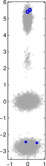
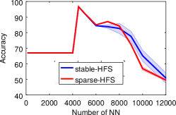
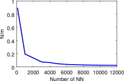
Figure 4: LABEL:sub@fig:gen-data The dataset of the synthetic experiment, LABEL:sub@fig:gen-error Accuracy of Stable-HFS and Sparse-HFS, LABEL:sub@fig:edge-ratio ratio of the number of edges $|\mathcal{H}|/|\mathcal{G}|$.

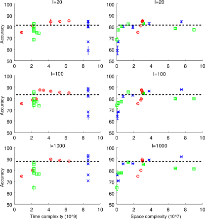
Figure 5: Accuracy vs complexity on the TREC 2007 SPAM Corpus for different number of labels. Legend: Sparse-HFS, EigFun, SubSampling, 1-NN

Spam-filtering dataset. We now evaluate the performance of our algorithm on the TREC 2007 Public Spam Corpus, that contains $n=75419$ raw emails labeled as either SPAM or HAM. The emails are provided as raw text and we applied standard NLP techniques to extract features vectors from it. In particular, we computed TF-IDF scores for each of the emails, with some additional cleaning in the form of a stop word list, simple stemming and dropping the 1% most common and most rare words. We ended up with $d=68697$ features, each representing a word present in some of the emails. From these features we proceeded to build a graph $\mathcal{G}$ where given two emails $\mathbf{x}_{i},\mathbf{x}_{j}$, the weight is computed as $a_{ij}=\exp(-\|\mathbf{x}_{i}-\mathbf{x}_{j}\|/2\sigma^{2})$, with $\sigma^{2}=3$. We consider the transductive setting, where the graph is fixed and known, but only a small random subset of $l=\{20,100,1000\}$ labels is revealed to the algorithm. As a performance measure, we consider the prediction accuracy over the whole dataset. We compare our method to several baselines. The most basic supervised baseline is 1-NN, which connects each node to the closest labeled node. The SubSampling algorithm selects uniformly $s$ nodes out of $n$, computes the HFS solution on the induced subgraph of $\mathcal{G}$ and assigns to each node outside of the subset the same label as the closest node in the subset. SubSampling’s complexity depends on the size $s$ of the subgraph and the number $k$ of neighbors retained when building the $k$-nn subgraph. The eigenfunction (EigFun) algorithm [11] tries to sidestep the computational complexity of finding an HFS solution on $\mathcal{G}$, by directly approximating the distribution that created the graph. Starting directly from the samples, each of the $d$ feature’s density is separately approximated using histograms with $b$ bins. From the histograms, $q$ empirical eigenfunctions (vectors in $\mathbb{R}^{n}$) are extracted and used to compute the final solution. We did not include Stable-HFS and Simple-HFS in the comparison because their $\mathcal{O}(m)$ space complexity made them unfeasible for this dataset. In Fig. 5, we report the accuracy of each method against the time and space complexity, where each separate point corresponds to a different choice in metaparameters (e.g. $k,q,s$). For EigFun, we use the same $b=50$ as in the original implementation, but we varied $q$ from 10 to 2000. For SubSampling, $s=15000$ and $k$ varies from 100 to 10000. We run Sparse-HFS on $\mathcal{G}$ setting $\varepsilon=0.9$, and changing the size $m$ of the input graph by changing the number of neighbours $k$ from 1000 to 7500. Since the actual running time and memory occupation are highly dependent on the implementation (e.g., EigFun is implemented in Matlab, while Sparse-HFS is Matlab/C), the complexities are computed using their theoretical form (e.g., $\mathcal{O}(m\log^{3}(n))$ for Sparse-HFS) with the values actually used in the experiment (e.g., $m=nk$ for a $k$-nn graph). All the complexities are reported in Fig. 3. The only exception is the number of edges in the sparsifier $N$ used in the space complexity of Sparse-HFS. Since this is a random quantity that holds only w.h.p. and that is independent from implementation details, we measured it empirically and used it for the complexities. For all methods we notice that the performance increases as the space complexity gets larger, until a peak is reached, while additional space induces the algorithms to overfit and reduces accuracy. For EigFun this means that a large number of eigenfunctions is necessary to accurately model the high dimensional distribution. And as theory predicts, SubSampling’s uniform sampling is not efficient to approximate the graph spectra, and a large subset of the nodes is required for good performance. Sparse-HFS’s accuracy also increases as the input graph gets richer, but unlike the other methods the space complexity does not change much. This is because the sparsifier is oblivious to the structure of the graph, and even if Sparse-HFS reaches its optimum performance for $k=3000$, the sparsifier contains roughly the same number of edges present as $k=1000$, and only 5% of the edges present in the input graph. Although preliminary, this experiment shows that the theoretical properties of Sparse-HFS translate into an effective practical algorithm which is competitive with state-of-the-art methods for large-scale SSL.

6 Conclusions and Future Work

We introduced Sparse-HFS, an algorithm that combines sparsification methods and efficient solvers for SDD systems to find approximate HFS solutions using only $\mathcal{O}(n\log^{2}(n))$ space instead of $\mathcal{O}(m)$. Furthermore, we show that the $\mathcal{O}(m\log^{3}(n))$ time complexity of the methods is only a $\operatorname*{polylog}$ term away from the smallest possible complexity $\Omega(m)$. Finally, we provide a bound on the generalization error that shows that the sparsification does not affect the asymptotic convergence rate of HFS. As such, the accuracy parameter $\varepsilon$ can be freely chosen to meet the desired trade-off between accuracy and space complexity. In this paper we relied on the sparsifier in [17] to guarantee a fixed space requirement, and the solver in [19] to efficiently compute the effective resistances. Both are straightforward to scale and parallelize [4], and the bottleneck in practice reduces to finding a fast sparse matrix-vector multiplication implementation for which many off-the-shelf solutions exist. We also remark that Sparse-HFS could easily accommodate any improved version of these algorithms and their properties would directly translate into the performance of Sparse-HFS. In particular [19] already mentions how finding an appropriate spanning tree (a low-stretch tree) and using it as the backbone of the sparsifier allows to reduce the space requirements of the sparsifier. Although this technique could lower the space complexity to $\mathcal{O}(n\log(n))$, it is not clear how to find such a tree incrementally. An interesting feature of Sparse-HFS is that it could be easily employed in online learning problems where edges arrive in a stream and intermediate solutions have to be computed over time. Since Sparse-HFS has a $\mathcal{O}(\log^{3}(n))$ amortized time per edge, it could compute intermediate solutions every $N$ edges without compromising its overall time complexity. The fully dynamic setting, where edges can be both inserted and removed, is an important extension where our approach could be further investigated, especially because it has been observed in several domains that graphs become denser as they evolve over time [21]. While sparsifiers have been developed for this setting (see e.g., [16]), current solutions would require $\mathcal{O}(n^{2}\operatorname*{polylog}(n))$ time to compute the HFS solution, thus making it unfeasible to repeat this computation many times over the stream. Extending sparsification techniques to the fully dynamic setting in a computationally efficient manner is an open problem.

References

- [1] Joshua Batson, Daniel A. Spielman, Nikhil Srivastava, and Shang-Hua Teng. Spectral sparsification of graphs: Theory and algorithms. Commun. ACM, 56(8):87–94, August 2013.
- [2] Mikhail Belkin, Irina Matveeva, and Partha Niyogi. Regularization and Semi-Supervised Learning on Large Graphs. In Proceedings of COLT, 2004.
- [3] Mikhail Belkin, Partha Niyogi, and Vikas Sindhwani. Manifold Regularization: A Geometric Framework for Learning from Labeled and Unlabeled Examples. Journal of Machine Learning Research, 7:2399–2434, 2006.
- [4] Guy E Blelloch, Ioannis Koutis, Gary L Miller, and Kanat Tangwongsan. Hierarchical diagonal blocking and precision reduction applied to combinatorial multigrid. In High Performance Computing, Networking, Storage and Analysis (SC), 2010 International Conference for, pages 1–12. IEEE, 2010.
- [5] Olivier Bousquet and André Elisseeff. Stability and generalization. The Journal of Machine Learning Research, 2:499–526, 2002.
- [6] Zhuhua Cai, Zekai J Gao, Shangyu Luo, Luis L Perez, Zografoula Vagena, and Christopher Jermaine. A comparison of platforms for implementing and running very large scale machine learning algorithms. In Proceedings of the 2014 ACM SIGMOD international conference on Management of data, pages 1371–1382. ACM, 2014.
- [7] Olivier Chapelle, Bernhard Schlkopf, and Alexander Zien. Semi-Supervised Learning. The MIT Press, 1st edition, 2010.
- [8] Avery Ching, Sergey Edunov, Maja Kabiljo, Dionysios Logothetis, and Sambavi Muthukrishnan. One trillion edges: graph processing at facebook-scale. Proceedings of the VLDB Endowment, 8(12):1804–1815, 2015.
- [9] Corinna Cortes, Mehryar Mohri, Dmitry Pechyony, and Ashish Rastogi. Stability of transductive regression algorithms. In Proceedings of ICML, pages 176–183. ACM, 2008.
- [10] Ran El-Yaniv and Dmitry Pechyony. Stable transductive learning. In Proceedings of COLT, pages 35–49. Springer, 2006.
- [11] Rob Fergus, Yair Weiss, and Antonio Torralba. Semi-Supervised Learning in Gigantic Image Collections. In Proceedings of NIPS, pages 522–530, 2009.
- [12] Jochen Garcke and Michael Griebel. Semi-supervised learning with sparse grids. In Proc. of the 22nd ICML Workshop on Learning with Partially Classified Training Data, 2005.
- [13] David F. Gleich and Michael W. Mahoney. Using local spectral methods to robustify graph-based learning algorithms. In Proceedings of the 21th ACM SIGKDD International Conference on Knowledge Discovery and Data Mining, KDD ’15, pages 359–368, New York, NY, USA, 2015. ACM.
- [14] Tony Jebara, Jun Wang, and Shih-Fu Chang. Graph construction and b-matching for semi-supervised learning. In Proceedings of the 26th Annual International Conference on Machine Learning, pages 441–448. ACM, 2009.
- [15] Ming Ji, Tianbao Yang, Binbin Lin, Rong Jin, and Jiawei Han. A Simple Algorithm for Semi-supervised Learning with Improved Generalization Error Bound. In Proceedings of ICML, June 2012.
- [16] Michael Kapralov, Yin Tat Lee, Christopher Musco, and Aaron Sidford. Single pass spectral sparsification in dynamic streams. In Foundations of Computer Science (FOCS), 2014 IEEE 55th Annual Symposium on, pages 561–570. IEEE, 2014.
- [17] Jonathan A. Kelner and Alex Levin. Spectral Sparsification in the Semi-streaming Setting. Theory of Computing Systems, 53(2):243–262, August 2013.
- [18] Ioannis Koutis, Alex Levin, and Richard Peng. Improved spectral sparsification and numerical algorithms for sdd matrices. In STACS’12 (29th Symposium on Theoretical Aspects of Computer Science), volume 14, pages 266–277. LIPIcs, 2012.
- [19] Ioannis Koutis, Gary L. Miller, and Richard Peng. A nearly-m log n time solver for SDD linear systems. In IEEE 52nd Annual Symposium on Foundations of Computer Science, FOCS, pages 590–598, 2011.
- [20] Sanjiv Kumar, Mehryar Mohri, and Ameet Talwalkar. Sampling methods for the Nyström method. J. Mach. Learn. Res., 13(1):981–1006, April 2012.
- [21] Jure Leskovec, Jon Kleinberg, and Christos Faloutsos. Graphs over time: densification laws, shrinking diameters and possible explanations. In Proceedings of the eleventh ACM SIGKDD international conference on Knowledge discovery in data mining, pages 177–187. ACM, 2005.
- [22] Wei Liu, Junfeng He, and Shih-Fu Chang. Large graph construction for scalable semi-supervised learning. In Proceedings of the 27th international conference on machine learning (ICML-10), pages 679–686, 2010.
- [23] Avneesh Saluja, Hany Hassan, Kristina Toutanova, and Chris Quirk. Graph-based semi-supervised learning of translation models from monolingual data. In Proceedings of the 52nd Annual Meeting of the Association for Computational Linguistics (ACL), Baltimore, Maryland, June, 2014.
- [24] Daniel A. Spielman and Nikhil Srivastava. Graph sparsification by effective resistances. SIAM Journal on Computing, 40(6):1913–1926, 2011.
- [25] Amarnag Subramanya and Partha Pratim Talukdar. Graph-based semi-supervised learning. Synthesis Lectures on Artificial Intelligence and Machine Learning, 8(4):1–125, 2014.
- [26] Ameet Talwalkar, Sanjiv Kumar, and Henry A. Rowley. Large-scale manifold learning. In Computer Vision and Pattern Recognition (CVPR), 2008.
- [27] Ivor W. Tsang and James T. Kwok. Large-scale sparsified manifold regularization. In Bernhard Schölkopf, John C. Platt, and Thomas Hoffman, editors, NIPS, pages 1401–1408. MIT Press, 2006.
- [28] Kai Yu and Shipeng Yu. Blockwise supervised inference on large graphs. In Proc. of the 22nd ICML Workshop on Learning, 2005.
- [29] Xiaojin Zhu. Semi-Supervised Learning Literature Survey. Technical Report 1530, U. of Wisconsin-Madison, 2008.
- [30] Xiaojin Zhu, Zoubin Ghahramani, and John Lafferty. Semi-Supervised Learning Using Gaussian Fields and Harmonic Functions. In Proceedings of ICML, pages 912–919, 2003.
- [31] Xiaojin Zhu and John D. Lafferty. Harmonic mixtures: combining mixture models and graph-based methods for inductive and scalable semi-supervised learning. In Proceedings of ICML, pages 1052–1059, 2005.