Maxwell field $\mathbf{E}$ in a two-dimensional polar fluid in the presence of an external field $\bm{\mathcal{E}}$ : a Monte-Carlo study

Abstract

We study a two-dimensional system of dipolar hard disks in the presence of a uniform external electric field $\bm{\mathcal{E}}$ by Monte Carlo simulations in a square with periodic boundary conditions. The study is performed in both the fluid at high temperature and the phase of living polymers at low temperature. In the considered geometry the macroscopic Maxwell field $\mathbf{E}$ is computed and found to be equal to the external field $\bm{\mathcal{E}}$ in both phases. The dielectric properties of the system in the liquid phase as well as in the polymeric phase are investigated.

I Introduction

We dedicate our contribution to the memory of George Stell with whom the Loup Verlet’s Orsay group has shared a long-lasting friendship.

This study is devoted to a Monte-Carlo (MC) simulation of a two-dimensional (2D) system made of identical dipolar hard disks (DHD) in the Euclidian plane $E_{2}$ in the presence of an uniform external electrostatic field $\bm{\mathcal{E}}$. The dipoles are assumed to be permanent and the configurational energy of $N$ dipolar molecules in $E_{2}$ reads as

$$H = \frac{1}{2}\sum_{i\neq j}^{N}v_{HS}(r_{ij})+\frac{1}{2}\mu^{2}\sum_{i\neq j}^{N}\frac{1}{r_{ij}^{2}}\left[\mathbf{s}_{i}\cdot\mathbf{s}_{j}-\frac{2(\mathbf{s}_{i}\cdot\mathbf{r}_{ij})(\mathbf{s}_{j}\cdot\mathbf{r}_{ij})}{r_{ij}^{2}}\right]$$

$$- \mu\sum_{i=1}^{N}\mathbf{s}_{i}\cdot\bm{\mathcal{E}}$$

$$\;.$$ (1)

In Eq. (I), $v_{HS}(r)$ is the hard disk potential of diameter $\sigma$. The second term is the contribution from the 2D dipole-dipole interaction where ${\bm{\mu}}_{i}=\mu\mathbf{s}_{i}$, $\mu$ permanent dipole moment, $\mathbf{s}_{i}$ unit vector in the direction of the dipole moment of particle $i$, $\mathbf{r}_{ij}=\mathbf{r}_{j}-\mathbf{r}_{i}$, the vector joining the centres of mass of the particles, and $r_{ij}=|\mathbf{r}_{ij}|$. Finally, the last term denotes the interaction energy of the dipoles with the external field $\bm{\mathcal{E}}$ which is assumed to be uniform. We note that the dipole-dipole interaction involved in Eq. (I) is derived from the solution of the 2D Laplace equation in the plane. This model was studied recently in the absence of $\bm{\mathcal{E}}$ by means of MC simulations performed on a sphere and in a square with periodic boundary conditions (PBC) Caillol_Weis . In both cases the laws of electrostatics governing the interactions in the considered geometries were scrupulously adopted yielding identical phase diagrams. At high temperature and moderate density an ordinary polar fluid is observed characterized by a dielectric constant $\epsilon$. In the low temperature, low density part of the phase diagram a phase of living polymers of dipoles organized into closed rings has been observed. At higher density the structure of this phase is characterized by an entangled structure of chains and rings and the dielectric constant $\epsilon$ is no more well-defined. It was found that the critical dipole moment $\mu_{c}^{*}$ at the transition from fluid to polymeric phase increases slightly with density.

In the presence of an applied field, in the low temperature phase the dipole moments are expected to align in the direction of the field, the tendency getting more effective as the strength of $\bm{\mathcal{E}}$ increases, first yielding roughly linear chains which ultimately will collapse into bundle-like structures at high density. As it is impossible to consider uniform fields on the sphere (without violating the laws of electrostatics, cf. Caillol ) we present here only simulations performed of DHD contained in a square with PBC.

II Electrostatics of $2D$ dipoles within periodical boundary conditions

Let us first recall some elements of electrostatics for a square of side $L$ along directions $Ox,Oy$ with PBC, which will be referred to as space $\mathcal{C}_{2}$ Caillol_Weis ; perram:81 ; morris:85 .

II.1 The dipolar Green’s function in $\mathcal{C}_{2}$

The electric field at point $\mathbf{r}_{1}=x_{1}\mathbf{e}_{x}+y_{1}\mathbf{e}_{y}$ ($(x_{1},x_{2})\in[-L/2,L/2]$, $(\mathbf{e}_{x},\mathbf{e}_{y})$ orthonormal basis of $\mathcal{C}_{2}$) created by a point dipole ${\bm{\mu}}_{2}$ located at point $\mathbf{r}_{2}=x_{2}\mathbf{e}_{x}+y_{2}\mathbf{e}_{y}$ of $\mathcal{C}_{2}$ is given by $2\pi\mathbf{G}_{0}(\mathbf{r}_{1},\mathbf{r}_{2})\cdot{\bm{\mu}}_{2}$ where $\mathbf{G}_{0}$ denotes the bare dipolar Green’s function and the dot a tensorial contraction (see e.g. Refs. Caillol ; Fulton_I ; Fulton_II ; Fulton_III ).

The Green’s function $\mathbf{G}_{0}$ depends on the considered geometry and is given in $\mathcal{C}_{2}$ by

$$\mathbf{G}_{0}(\mathbf{r}_{1},\mathbf{r}_{2})\equiv\mathbf{G}_{0}(\mathbf{r}_{12})=\dfrac{1}{2\pi}\dfrac{\partial}{\partial\mathbf{r}_{12}}\dfrac{\partial}{\partial\mathbf{r}_{12}}\psi(\mathbf{r}_{12})\;,$$ (2)

where $\psi(\mathbf{r})$ is the periodic Ewald potential. The latter satisfies Poisson’s equation in $\mathcal{C}_{2}$, i.e.

$$\Delta\psi(\mathbf{r})=-2\pi[\delta_{\mathcal{C}_{2}}(\mathbf{r})-\dfrac{1}{L^{2}}]\;,$$ (3)

where

$$\delta_{\mathcal{C}_{2}}(\mathbf{r})= \sum_{\mathbf{n}}\delta^{(2)}(\mathbf{r}-L\mathbf{n})\,,$$

$$= \dfrac{1}{L^{2}}\sum_{\mathbf{k}}\exp(i\mathbf{k}\cdot\mathbf{r})\,,$$ (4)

is the periodical Dirac’s comb. In Eqs. (II.1) $\mathbf{k}=(2\pi/L)\mathbf{n}$ where $\mathbf{n}$ is a $2D$ vector with integer components $(n_{x},n_{y})$ in the basis $(\mathbf{e}_{x},\mathbf{e}_{y})$ . One notes that $\psi(\mathbf{r})$ identifies with the potential created by a unit point charge immersed in a uniform neutralizing background of charge density $-1/L^{2}$. Expanding $\psi(\mathbf{r})$ and $\mathbf{G}_{0}(\mathbf{r})$ in Fourier series one finds

$$\psi(\mathbf{r})= \dfrac{2\pi}{L^{2}}\sum_{\mathbf{k}\neq\mathbf{0}}\dfrac{\exp(i\mathbf{k}\cdot\mathbf{r})}{\mathbf{k}^{2}}\,,$$ (5a)

$$\mathbf{G}_{0}(\mathbf{r})= -\dfrac{1}{L^{2}}\sum_{\mathbf{k}\neq\mathbf{0}}\widehat{\mathbf{k}}\widehat{\mathbf{k}}\exp(i\mathbf{k}\cdot\mathbf{r})\;,$$ (5b)

where $\widehat{\mathbf{k}}=\mathbf{k}/\Arrowvert\mathbf{k}\Arrowvert$. Some comments on the previous developments are in order:

• (i) It follows from Eq. (5b) that

  $$\int_{\mathcal{C}_{2}}\;d\mathbf{r}_{2}\,\mathbf{G}_{0}(\mathbf{r}_{1},\mathbf{r}_{2})=\mathbf{0}\;,$$ (6)

  and therefore the electric field created by a uniform polarization $\mathbf{P}$ is zero (see Sec. (II.3)).

• (ii) Clearly $\mathbf{G}_{0}(\mathbf{r})$ exhibits the same singularity for $\mathbf{r}\to\mathbf{0}$ as the Green’s function of the infinite Euclidean plane ${\bba R}^{2}$, i.e.Caillol ; Fulton_I ; Fulton_II ; Fulton_III ; Jackson

  $$\mathbf{G}_{0}(\mathbf{r}) =\mathbf{G}_{0}^{\delta}(\mathbf{r})-\,\frac{1}{2}\,\delta(\mathbf{r})\,\mathbf{U}\;,$$ (7a)

  $$\mathbf{G}_{0}^{\delta}(\mathbf{r})=\begin{cases}\mathbf{G}_{0}(\mathbf{r})\;&,\text{ for }r>\delta\;,\\ 0\;&,\text{ for }r<\delta\;,\end{cases}$$ (7b)

  where $\mathbf{U}=\mathbf{e}_{x}\mathbf{e}_{x}+\mathbf{e}_{y}\mathbf{e}_{y}$ is the unit dyadic tensor. In Eqs. (7) $\delta$ is an arbitrary small cutoff ultimately set to zero if point dipoles are to be considered. It must be understood that any integral involving $\mathbf{G}_{0}^{\delta}$ must be calculated with $\delta\neq 0$ and then taking the limit $\delta\to 0$. In the presence of hard cores, as in the DHD fluid, the point dipoles can be replaced by a continuous charge distribution of symmetry axis $\mathbf{s}$ and charge density $\propto\mathbf{s}\cdot\mathbf{r}$. In that case $\delta$ can be chosen to take any value $0<\delta\leq\sigma/2$.

• (iii) The interaction energy of two dipoles of $\mathcal{C}_{2}$ is given by $-2\pi{\bm{\mu}}_{1}\cdot\mathbf{G}_{0}(\mathbf{r}_{1},\mathbf{r}_{2})\cdot{\bm{\mu}}_{2}$. As well-known, expression (5b) cannot be handled in a straightforward way in MC simulations since it converges very slowly. This Fourier series is then splitted into two series, one in direct space, the other in Fourier space, both with good convergence properties. In that way one obtains the dipolar Ewald potential which is detailed in Ref. Caillol_Weis and which was used in the simulations reported in this paper.

II.2 Linear distributions of dipoles in $\mathcal{C}_{2}$

We consider a line of length $L$, parallel to axis $Oy$ of a square with PBC, which bears a continuous distribution of dipoles $d\bm{\lambda}=(\lambda_{x}\mathbf{e}_{x}+\lambda_{y}\mathbf{e}_{y})dy$ where the components $(\lambda_{x},\lambda_{y})$ are constants. Without loss of generality the equation of the line can be chosen as $x=0$. The electric field $d\bm{\mathcal{E}}$ created by this infinitesimal dipole at point $\mathbf{r}$ is given by

$$d\bm{\mathcal{E}} =2\pi\mathbf{G}_{0}(\mathbf{r})\cdot d\bm{\lambda}\,,$$

$$=-\frac{2\pi}{L^{2}}\sum_{\mathbf{k}\neq\mathbf{0}}\;\frac{\mathbf{k}\mathbf{k}}{k_{x}^{2}+k_{y}^{2}}\exp(i(k_{x}x+k_{y}y))\cdot(\lambda_{x}\mathbf{e}_{x}+\lambda_{y}\mathbf{e}_{y})dy\,,$$

$$=-\frac{2\pi}{L^{2}}\sum_{\mathbf{k}\neq\mathbf{0}}\;\frac{\mathbf{k}}{k_{x}^{2}+k_{y}^{2}}\exp(i(k_{x}x+k_{y}y))(\lambda_{x}k_{x}+\lambda_{y}k_{y})dy\,.$$ (8)

The total field of the line is obtained by integration

$$\bm{\mathcal{E}} =2\pi\int_{-L/2}^{L/2}d\bm{\mathcal{E}}\,.$$

$$=-\frac{2\pi\lambda_{x}}{L^{2}}\sum_{\mathbf{k}\neq\mathbf{0}}\;\frac{k_{x}\mathbf{k}}{k_{x}^{2}+k_{y}^{2}}\exp(ik_{x}x)L\delta_{k_{y},0}\,,$$

$$=-\frac{2\pi\lambda_{x}}{L}\sum_{k_{x}\neq 0}\exp(ik_{x}x)\mathbf{e}_{x}\;,$$

$$=-2\pi\lambda_{x}\left[\delta(x)-\frac{1}{L}\right]\mathbf{e}_{x}\;.$$ (9)

Eq. (II.2) shows that the field of a uniform distribution of dipoles aligned along the line $x=0$ ($\lambda_{x}=0$) vanishes exactly. This result should be compared with the expression of the field created by an infinite linear chain of point dipoles, each with dipole moment $\mu\mathbf{e}_{y}$, all aligned along the $Oy$ axis with spacing $2a$ given in Ref. Toor . The latter is expressed as a series, the dominant term of which behaves as $\propto(\mu/a^{2})\exp(-\pi|x|/a)\cos(\pi y/a)$. With the correspondence $\mu=2\lambda_{y}a$ and in the limit of a continuous distribution, i.e. $a,\mu\to 0$ with $\lambda_{x}$ fixed, this dominant term vanishes in agreement with our result. These results suggest that in the polymeric phase and in the presence of a sufficiently large external field the chains of dipoles aligned along the field do not contribute significantly to the Maxwell field. This point has been checked in our simulations and is discussed in Sec. (III).

The expression (II.2) of $\mathcal{E}$ also shows that, apart from the singularity $-2\pi\lambda_{x}\delta(x)\mathbf{e}_{x}$, a uniform electric field parallel to the axis $Ox$ of strength $2\pi\lambda_{x}/L$ can be generated by a uniform distribution of dipoles perpendicular to the line ($\lambda_{y}=0$). In passing we note that the delta singularity has no effect in actual simulations since the condition $x=0$, of measure zero, is never obtained. We also remark that $\lambda_{x}$ being fixed, the field vanishes in the limit $L\to\infty$ as it should be, since then the result of the Euclidean plane ${\bba R}^{2}$ with free boundaries at infinity should be recovered. The electrostatic potential obtained by integration, is found, up to an arbitrary additional constant, to be

$$V(x) =\begin{cases}=\pi\lambda_{x}-\dfrac{2\pi}{L}\lambda_{x}x\text{ , for }x>0\\ =-\pi\lambda_{x}-\dfrac{2\pi}{L}\lambda_{x}x\text{ , for }x<0\,,\end{cases}$$ (10)

yielding the expected discontinuity of the potential across a dipole layerJackson

$$V(0+)-V(0-)=2\pi\lambda_{x}\,.$$ (11)

These results can be extended to the $3D$ case (with $2\pi$ replaced by $4\pi$) where one should consider instead a planar uniform layer of dipoles aligned along the normal to the square $x=0$ of the cube $\mathcal{C}_{3}$. We stress that it seems to be the only way to generate a uniform electrostatic field within PBC cubic geometries.

II.3 The Maxwell field in $\mathcal{C}_{2}$

At thermal equilibrium the Maxwell field $\mathbf{E}(\mathbf{r})$ is the sum of the external field $\bm{\mathcal{E}}(\mathbf{r})$ and the field created by the dipoles $\mathbf{E}_{d}(\mathbf{r})=<\widehat{\mathbf{E}}_{d}(\mathbf{r})>$. It follows from Sec. (II.1) that, in a given configuration of $N$ dipoles in the canonical ensemble, the microscopic field $\widehat{\mathbf{E}}_{d}(\mathbf{r})$ is given by

$$\widehat{\mathbf{E}}_{d}(\mathbf{r})=2\pi\int_{\mathcal{C}_{2}}d\mathbf{r}^{{}^{\prime}}\mathbf{G}_{0}(\mathbf{r},\mathbf{r}^{{}^{\prime}})\cdot\widehat{\mathbf{P}}(\mathbf{r}^{{}^{\prime}})\;,$$ (12)

where the microscopic polarization at point $\mathbf{r}$ reads

$$\widehat{\mathbf{P}}(\mathbf{r})=\sum_{i=1}^{N}\bm{\mu}_{i}\delta_{\mathcal{C}_{2}}(\mathbf{r}-\mathbf{r}_{i})\;.$$ (13)

At equilibrium we thus have

$$\mathbf{E}(\mathbf{r})=\bm{\mathcal{E}}(\mathbf{r})+2\pi\int_{\mathcal{C}_{2}}d\mathbf{r}^{{}^{\prime}}\mathbf{G}_{0}(\mathbf{r},\mathbf{r}^{{}^{\prime}})\cdot\mathbf{P}(\mathbf{r}^{{}^{\prime}})\;,$$ (14)

where the macroscopic polarization $\mathbf{P}(\mathbf{r})=<\widehat{\mathbf{P}}(\mathbf{r})>$.

For a fluid in a uniform external field $\bm{\mathcal{E}}$ the polarization $\mathbf{P}$ is uniform and, for a sufficiently low field strength, $2\pi\mathbf{P}=(\epsilon-1)\mathbf{E}$, which defines the dielectric constant $\epsilon$. As well known Jackson the relation between the Maxwell field and the external field depends on the geometry. For instance, in the plane ${\bba R}^{2}$ with free boundaries at infininity we have $\mathbf{E}=\bm{\mathcal{E}}/\epsilon$ while, in $\mathcal{C}_{2}$ we have

$$\mathbf{E}_{d} =\left[2\pi\int_{\mathcal{C}_{2}}d\mathbf{r}^{{}^{\prime}}\mathbf{G}_{0}(\mathbf{r},\mathbf{r}^{{}^{\prime}})\right]\cdot\mathbf{P}\,,$$

$$=\mathbf{0}\;,$$ (15)

as a consequence of Eq. (6) from which it follows that $\mathbf{E}=\bm{\mathcal{E}}$ and therefore $2\pi\mathbf{P}=(\epsilon-1)\bm{\mathcal{E}}$.

III MC data analysis

For the present planar system the MC simulations were performed in a square of surface $A=L^{2}$ with PBC for $N=1024$ hard disks carrying a dipole moment, in reduced units, $\mu^{*}=\mu/\sqrt{kT\sigma^{2}}$ varying between $\mu^{*}=1.5$ and $2.75$. The densities, in reduced units, were taken in the range $\rho^{*}=\rho\sigma^{2}$ from 0.1 to 0.3. The energy $E$ of the system in the presence of the external field ${\bf\cal E}$ is calculated, taking into account the PBC, by the Ewald summation technique explicated in Refs Caillol_Weis ; perram:81 ; morris:85 . The expression at point ${\bf r}$ of the microscoipic field $\widehat{{\bf E}}_{d}({\bf r})$ due to the $N$ dipoles ${\bm{\mu}}^{*}_{i}=\mu^{*}{\bf s}_{i}$ is thus given by

$$\widehat{{\bf E}}_{d}({\bf r}) = 2\pi\sum_{i=1}^{N}\mathbf{G}_{0}(\mathbf{r},\mathbf{r}_{i})\cdot{\bm{\mu}}^{*}_{i}$$ (16)

$$\simeq \sum_{i=1}^{N}\Big{\{}{({\bf r-r}_{i})}{\frac{2\,\exp(-\alpha^{2}|{\bf{r}-\bf{r}_{i}}|^{2})}{|{\bf{r}-\bf{r}_{i}}|^{2}}}({\frac{1}{|{\bf{r}-\bf{r}_{i}}|^{2}}+\alpha^{2}})({\bf{r}-\bf{r}_{i}}).{\bm{\mu}}^{*}_{i}-{\frac{\exp(-\alpha^{2}|{\bf{r}-\bf{r}_{i}}|^{2})}{|{\bf{r}-\bf{r}_{i}}|^{2}}}{\bm{\mu}}^{*}_{i}\Big{\}}$$

$$+ {\frac{2\,\pi}{A}}\sum_{{\bf k\neq 0}}{{\bf k}}{\frac{\exp(-|{\bf k}|^{2}/(4\alpha^{2}))}{|{\bf k}|^{2}}}\sum_{i}\exp(-i{\bf k}.{\bf r}_{i})\exp(i{\bf k}.{\bf r}){{\bm{\mu}}^{*}_{i}}.{\bf k}\,,$$

where we have reported in the second line of Eq. (16) the Ewald expression used in our simulations. The parameter $\alpha$ regulates the rate of convergence of the sums in direct and Fourier space.

At equilibrium the Maxwell, or macroscopic field is defined as

$$\mathbf{E}=\bm{\mathcal{E}}+\left\langle\widehat{{\bf E}}_{d}\right\rangle\,,$$ (17)

where the brackets denote a canonical average, while the macroscopic polarization is the canonical average of $\widehat{{\bf P}}({\bf r})=\mu^{*}\sum_{i}{\bf s}_{i}\delta({\bf r}-{\bf r}_{i})$. In the region of the phase diagram where it is a defined quantity and in the limit of small fields, the dielectric constant $\epsilon$ of the system can be obtained, as discussed in Sec. (II.3), through $2\pi<\widehat{\mathbf{P}}({\bf r})>=(\epsilon-1)<\widehat{\mathbf{E}}({\bf r})>$.

In the simulations the external field ${\bf{\cal E}}$ is chosen parallel to the $Oy$ axis and the microscopic field $\widehat{{\bf E}}_{d}({\bf r})$ is calculated for an ensemble of $N_{c}=65{\rm x}65=4225$ points located at the grid points of a square lattice. It is calculated even if the point ${\bf r}$ is inside the hard core of the disk. Hence the possibility of a rare but large contribution to $\widehat{{\bf E}}_{d}^{\delta}({\bf r})$, which is avoided by setting to zero the values $r<\delta=0.1\sigma$ in the tabulation of the gaussian functions in Eq.(16). Clearly it amounts to compute

$$\widehat{{\bf E}}_{d}^{\delta}({\bf r})=2\pi\sum_{i=1}^{N}\mathbf{G}_{0}^{\delta}(\mathbf{r},\mathbf{r}_{i})\cdot{\bm{\mu}}^{*}_{i}$$ (18)

where the truncated Green function $\mathbf{G}_{0}^{\delta}$ is that of Eq. (7b). It follows then from Eq. (7a) that

$$<\widehat{{\bf E}}_{d}({\bf r})> = <\widehat{{\bf E}}_{d}^{\delta}({\bf r})>-\pi<\widehat{{\bf P}}({\bf r})>\,.$$ (19)

The Maxwell field has been computed from Eq. (19) for the thermodynamic states given in Table I. For dipole moment $\mu^{*}=1.5$, and all densities considered, the system reaches equilibrium after of the order of $10^{5}$ MC trial moves per particle and about $10^{6}$ MC trial moves per particle appear sufficient to evaluate the canonical averages with a precision of $1\%$. Such a sampling is also sufficient to achieve average values of $\widehat{{\bf E}}_{d}^{\delta}({\bf r}_{s})$ at the different grid points $1,\,2,\,...\,,s,\,...\,,N_{c}$ independent of ${\bf r}_{s}$ for all considered values of the external field.

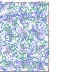
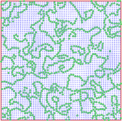
Figure 1: Snapshots of configurations of $1024$ dipolar discs at $\mu^{*}=2.5$, $\rho^{*}=0.3$ and ${\cal E}_{y}=0.1$. The blue lines indicate the values and orientations of the average values of $\widehat{{\bf E}}_{d}^{\delta}({\bf r}_{s})$ at the different points ${\bf r}_{s}$. Left : after $3\,10^{5}$ trial moves per particle. Right : after $2\,10^{7}$ trial moves per particle, the computed values $<\widehat{{\bf E}}_{d}^{\delta}({\bf r}_{s})>$ are quasi-uniform.

For dipole moments $\mu^{*}=2.5$ or $2.75$, a configuration of the system is typically characterized by the formation of chains and rings. Such an arrangement of the disks evolves to a different but similar arrangement only within $10^{5}$ trial moves per particle and therefore of the order of $10^{7}$ trial moves per particle are necessary for the estimate of the canonical averages and to obtain an average value of $\widehat{{\bf E}}_{d}^{\delta}({\bf r}_{s})$ quasi-independent of ${\bf r}_{s}$. Figures 1 provides snapshots of such an evolution at ${\cal E}_{y}=0.1$ for $\mu^{*}=2.5$ and $\rho^{*}=0.3$.

The results of Table I show that for all thermodynamic states considered the average value $<\widehat{{\bf E}}^{d}({\bf r})>$ $\simeq 0$ as $-\pi<\widehat{{\bf P}}({\bf r})>$ cancels $<\widehat{{\bf E}}_{d}^{\delta}({\bf r})>$ in the limit of statistical errors. This result allows to obtain two estimates of the dielectric constant $\epsilon$ in the limit of small external fields, one, denoted $\epsilon_{\cal E}$, by

$$\epsilon_{\cal E}-1=2\pi<\widehat{P}_{y}({\bf r})>/{\cal E}_{y}$$ (20)

the other, denoted $\epsilon_{P}$, by

$$(\epsilon_{P}-1)/(\epsilon_{P}+1)=\pi<\widehat{P}_{y}({\bf r})>/({\cal E}_{y}+<\widehat{E}_{d,y}^{\delta}({\bf r})>)$$ (21)

${\cal E}_{y}$	$\rho^{*}$	$\mu^{*}$	$<\widehat{E}_{d,y}^{\delta}({\bf r})>$	$-\pi<\widehat{P}_{y}({\bf r})>$	$<\widehat{E}_{y}({\bf r})>$	$\epsilon_{\cal E}$	$\epsilon_{P}$
0.0000	0.10	2.75	0.400E-03	-0.106E-04	0.389E-03
0.0000	0.10	2.75	0.552E+00	-0.552E+00	-0.368E-03
0.1000	0.10	2.75	0.323E+00	-0.323E+00	0.253E-03
0.1000	0.10	2.75	0.710E+00	-0.711E+00	-0.691E-03
0.0050	0.30	2.50	0.906E-01	-0.900E-01	0.565E-03	0.370E+02	0.334E+02
0.0075	0.30	2.50	0.162E+00	-0.162E+00	-0.128E-04	0.442E+02	0.442E+02
0.0100	0.30	2.50	0.178E+00	-0.179E+00	-0.968E-03	0.368E+02	0.406E+02
0.0125	0.30	2.50	0.220E+00	-0.220E+00	-0.206E-03	0.363E+02	0.369E+02
0.0150	0.30	2.50	0.268E+00	-0.268E+00	-0.687E-03	0.368E+02	0.385E+02
0.0175	0.30	2.50	0.330E+00	-0.330E+00	-0.144E-03	0.387E+02	0.391E+02
0.0250	0.10	1.50	0.124E-01	-0.124E-01	-0.298E-04	0.199E+01	0.199E+01
0.0500	0.10	1.50	0.248E-01	-0.248E-01	-0.142E-04	0.199E+01	0.199E+01
0.0750	0.10	1.50	0.373E-01	-0.373E-01	-0.342E-05	0.199E+01	0.199E+01
0.1000	0.10	1.50	0.494E-01	-0.494E-01	0.676E-05	0.199E+01	0.199E+01
0.2000	0.10	1.50	0.962E-01	-0.963E-01	-0.432E-04	0.196E+01	0.196E+01

Table 1: Maxwell field and dielectric constant for thermodynamics states at low and high reduced dipole moments and for densities $0.1$ and $0.3$. $\epsilon_{\cal E}$ and $\epsilon_{P}$ are computed from Eqs. (20 ) and (21 ), respectively. At $\mu^{*}=2.75$, the evaluation of $\epsilon$ is precluded by the metastability of the thermodynamic states.

.

For $\rho^{*}=0.1$ and $\mu^{*}=1.5$ the two estimates of $\epsilon$ are in excellent agreement for all values ${\cal E}_{y}<0.2$. This value of $1.97$ is also in agreement with the value $2.01$ determined by the fluctuation formula Caillol_Weis at ${\cal E}=0$, $\epsilon-1=\pi<\widehat{{\bf M}}^{2}>/A$ where $\widehat{{\bf M}}=\mu^{*}\sum_{i}\mathbf{s}_{i}$. At $\rho^{*}=0.3$ and $\mu^{*}=2.5$ the estimated value of $\epsilon$ is equal to $\sim 38.0\pm 2.0$ if $0.01<{\cal E}_{y}<0.02$; for ${\cal E}_{y}<0.01$ the estimated values lie between $43.0$ and $33.0$, a dispersion corresponding to the fact that after more then $10^{7}$ trial moves per particle the statistical error on $<\widehat{P}_{y}({\bf r})>$ remains of the order of $10\%$. The estimated value is in agreement with that, $38.0\pm 1.0$, obtained from the fluctuation formula.

At $\rho^{*}=0.1$ and $\mu^{*}=2.75$, the field $<\widehat{E}_{d,y}({\bf r})>$ is also zero in the limit of statistical errors, demonstrating that within the performed trial moves, the values of $<\widehat{P}_{y}({\bf r})>$ and $<\widehat{E}_{d,y}^{\delta}({\bf r})>$ remain coherent such that the Maxwell field remains equal to the external field. However, it is manifest that for $\mu^{*}=2.75$, sampling of configurations is affected by strong metastability as shown by comparison of the average polarizations, obtained with ${{\cal E}_{y}}=0$ and $3\,10^{7}$ trials per particle, using different initial conditions. In one of the runs, starting from an unpolarized initial configuration, the average final polarization is $\sim 10^{-5}$ (first line of Table I) , whereas in a run starting from an initial configuration with a polarization close to the maximal polarization $0.275$, the average final polarization is equal to $\sim 0.175$ (second line of Table I). Snapshots of characteristic configurations for these two states are given in Figure 2. Similarly at ${{\cal E}_{y}}=0.1$, for two runs with different initial configuration, the polarizations seem stable for a sampling of $3\,10^{7}$ trials per particle, with values $0.102$ and $0.226$, respectively. This important metastability affecting the polarization values precludes a reliable calculation of $\epsilon$ from Eqs. (20 ) or (21 ).

IV Conclusion

A 2D dipolar system with periodic boundary conditions in the presence of a uniform external field behaves according to the laws of electrostatics. This result allows to show by numerical simulation that the Maxwell field inside the system is equal to the applied external field even if the system is highly polarized and also for stable or possibly metastable states where the configurations of the system are dominated by chaines and rings. This equality between Maxwell and external field does, however, not permit to overcome the difficulties inherent in the determination of the dielectric constant of the system at low temperature. Indeed, at these temperatures the simulations are affected by important metastability which precludes a unambiguous determination of the stable thermodynamic state.

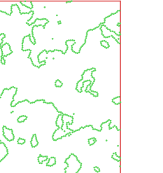
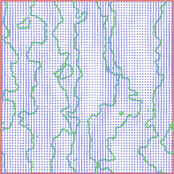
Figure 2: Snapshots of configurations of $1024$ dipolar discs at $\mu^{*}=2.75$, $\rho^{*}=0.1$ and ${\cal E}_{y}=0$ after $3\,10^{7}$ moves per particle. Left : final configuration for a run starting from an initial unpolarized configuration; in this state $<\widehat{P}_{y}({\bf r)}>\simeq 0$ $<\widehat{{E}}_{d,y}^{\delta}({\bf r}_{s})>\simeq 0$. Right : final configuration for a run starting from an initial polarized configuration; in this state the average polarization is $<\widehat{P}_{y}({\bf r)}>=0.175$ and $<\widehat{{E}}_{d,y}^{\delta}({\bf r}_{s})>=-0.552$.

References

- (1) Caillol J-M and Weis J-J 2015 Mol. Phys. 113 2487
- (2) Caillol J-M 2015 J. Chem. Phys. 142 154505
- (3) Perram J W and de Leeuw S W 1981 Physica 109A 237
- (4) Morriss G P and Perram J W 1985 Physica 129A 395
- (5) Fulton R L 1978 J. Chem. Phys. 68 3089
- (6) Fulton R L 1978 J. Chem. Phys. 68 3095
- (7) Fulton R L 1983 J. Chem. Phys. 78 6865
- (8) Jackson J D Classical Electrodynamics (John Wiley & Sons, New York, 1962)
- (9) William R. Toor W R 1993 J. of Colloid and Interfac. Sci. 156, 335