Determining Type Ia Supernovae Host galaxy extinction probabilities and a statistical approach to estimating the absorption-to-reddening ratio $R_{V}$

Abstract

We investigate limits on the extinction values of Type Ia supernovae to statistically determine the most probable color excess, E(B-V), with galactocentric distance, and use these statistics to determine the absorption-to-reddening ratio, $R_{V}$, for dust in the host galaxies. We determined pixel-based dust mass surface density maps for 59 galaxies from the Key Insight on Nearby Galaxies: a Far-Infrared Survey with Herschel (KINGFISH, Kennicutt et al. (2011)). We use Type Ia supernova spectral templates (Hsiao et al., 2007) to develop a Monte Carlo simulation of color excess E(B-V) with $R_{V}$ = 3.1 and investigate the color excess probabilities E(B-V) with projected radial galaxy center distance. Additionally, we tested our model using observed spectra of SN 1989B, SN 2002bo and SN 2006X, which occurred in three KINGFISH galaxies. Finally, we determined the most probable reddening for Sa-Sap, Sab-Sbp, Sbc-Scp, Scd-Sdm, S0 and Irregular galaxy classes as a function of $R/R_{25}$. We find that the largest expected reddening probability are in Sab-Sb and Sbc-Sc galaxies, while S0 and Irregulars are very dust poor. We present a new approach for determining the absorption-to-reddening ratio $R_{V}$ using color excess probability functions, and find for a sample of 21 SNe Ia observed in Sab-Sbp galaxies, and 34 SNe in Sbc-Scp, an $R_{V}$ of 2.71 $\pm$ 1.58 and $R_{V}$ = 1.70 $\pm$ 0.38 respectively.

1. Introduction

Because Type Ia supernovae (SNe Ia) are bright, they are good standard candles and probably the most accurate distance indicators on cosmological scales. Although SNe Ia are not equally bright there is a known correlation between their peak brightness and the width of their light curves (Phillips, 1993), which is used to standardize the ”Branch” normal SNe Ia. However, there are SNe Ia that appear dimmer and redder than the Branch normals, either because they are intrinsically different, or because they suffer greater host galaxy extinction. One of the largest sources of uncertainty in Type Ia SNe photometric measurements is the extinction due to the host galaxy, which affects the accuracy and precision of constructed Hubble diagrams. In turn, this limits the accuracy of the measurement of the dark energy parameters. Sullivan et al. (2006) examined the effect of host galaxy morphology on the Hubble diagram of SNe Ia. They found that elliptical galaxy SNe Hubble diagram had less scatter than spiral galaxy SNe.

Understanding the effect of dust extinction on SNe Ia is essential for accurate measurement of cosmological parameters and the expansion history of the Universe (Riess et al., 1998; Perlmutter et al., 1999). Extinction $A_{V}$, is determined from the reddening law $E(B-V)=A_{V}/R_{V}$, where the color excess E(B-V) depends on the properties of dust. If these are uncertain and/or evolve with redshift, the extinction, and thus the SNe Ia brightness, might be systematically wrong.

Previous studies of the extinction from SNe Ia (summarized in Table 1) yielded diverse values of the absorption to reddening ratio, $R_{V}$, ranging from $R_{V}$ = 1 to $R_{V}$ = 3.5. For comparison, the average value for the Milky Way is $R_{V}$ = 3.1. These studies used a variety of methods to calculate $R_{V}$, most of them are variants on multi-color light curve fitting.

Branch & Tammann (1992) calculated $\langle R_{B}\rangle$ = 2.0 from measurements of six SNe Ia in the Virgo cluster, and $\langle R_{B}\rangle$ = 1.2 from three pairs of SNe which occurred in the same galaxies (note that $R_{B}$ = $R_{V}$ + 1). They also determined $R_{B}$ = 1.3 $\pm$ 0.2 from a least square solution for a sample of 17 nearby SNe Ia ($\lesssim$ 4000 $km$ $s^{-1}$) in the Hubble diagram, using the SNe Ia sample from Miller & Branch (1990). Phillips et al. (1999) developed a method to estimate the extinction of low redshift SNe Ia (0.01 $\lesssim$ z $\lesssim$ 0.1) based on the observational coincidence that the B-V evolution between 30 and 90 days after the peak luminosity in V is similar for all SNe Ia, regardless of light curve shape. They obtain $R_{V}$ = 3.5 $\pm$ 0.4 for a sample of 49 SNe Ia.

Altavilla et al. (2004) estimated $R_{B}$ = 3.5 from light curves of 73 SNe with z $\lesssim$ 0.1. Reindl et al. (2005) calculated $R_{V}$ = 2.65 $\pm$ 0.15 for 111 SNe Ia with recession velocities between 3000 $km$ $s^{-1}$ and 20000 $km$ $s^{-1}$, exploiting the $M_{B}$(max) vs. E(B-V) correlation. Riess et al. (1996b) found a value of $R_{V}$ = 2.55 $\pm$ 0.30, derived using a multi-color light-curve shape (MLCS) method for a sample of 20 Ia SNe with z $\lesssim$ 0.1. Conley et al. (2007) used four different light curve fitting packages, and determined $R_{V}$ $\sim$ 1 for a sample of 61 SNe with v $\lesssim$ 40000 $km$ $s^{-1}$. To explain their low $R_{V}$, Conley et al. (2007) suggest that a more complicated model of intrinsic SN colors is required, which goes beyond single light-curve shape-color relation, or that dust in the host galaxies of the Ia SNe is quite different compared to Milky Way dust.

Hicken et al. (2009a) combined the CfA3 SNe Ia (Hicken et al., 2009b) with the UNION set (Kowalski et al., 2008) to determine the equation of state parameter w. They use four different light curve fitters and found lower Hubble residuals for $R_{V}$ = 1.7 compared to $R_{V}$ = 3.1, i.e. the higher $R_{V}$ value overestimates host galaxy extinction.

In a different approach, Mandel et al. (2011) constructed a statistical model for Type Ia SNe light curves from the visible through the infrared, and applied it to data of 127 SNe from three surveys (PAIRITEL, CfA3, Carnegie Supernova Project) and from the literature. They calculated $R_{V}$ $\approx$ 2.5 $-$ 2.9 for $A_{V}$ $\lesssim$ 0.4, while for higher extinctions, $A_{V}$ $\gtrsim$ 1, values of $R_{V}<$ 2 are calculated. Kessler et al. (2009) determined $R_{V}$ = 2.18 $\pm$ 0.14(stat) $\pm$ 0.48(syst) by matching observed and predicted SN Ia colors for 103 SNe with 0.04 $<$ z $<$ 0.42. Folatelli et al. (2010) found $R_{V}$ $\approx$ 1.7 when using 17 low-redshift (z $<$ 0.08) SNe Ia monitored by the Carnegie Supernova Project, but obtain $R_{V}$ $\approx$ 3.2 when two highly reddened SNe are excluded.

Lampeitl et al. (2010) from a sample of 361 SDSS-II SNe, z $<$ 0.21, utilizing two light curve methods, found that SNe Ia in passive host galaxies favor a dust law of $R_{V}$ = 1.0 $\pm$ 0.2, while SNe Ia in star-forming hosts require $R_{V}$ = $1.8^{+0.2}_{-0.4}$.

Nobili & Goobar (2008) found that SNe Ia color depends on the light curve shape, such that SNe Ia with fainter, narrower light curves are redder than those with brighter, broader light curves (cf. Phillips (1993), Riess et al. (1996a), Phillips et al. (1999), Nugent et al. (2002a) and Nobili et al. (2003)). They correct SNe light curves for this intrinsic color difference, and then derive host galaxy reddening. They obtain $R_{V}$ = 1.75 $\pm$ 0.27 for 80 low redshift ($\lesssim$ 0.1) SNe Ia with $E(B-V)\leq 0.7$ mag, but find that a subset of 69 SNe that have modest reddening, $E(B-V)<0.25$ mag, have significantly smaller $R_{V}$ $\sim$ 1.

Using a Monte Carlo simulation of circumstellar dust around the supernova location, Goobar (2008) determined $R_{V}$ $\sim$ 1.5 $-$ 2.5 for SNe Ia. One of Goobar’s motivations in undertaking this study was the observed steeper dependence with wavelength of the total to selective extinction seen in SNe Ia by e.g. Wang (2005). Using Draine’s Milky Way dust models (Draine, 2003b) and the Weingartner & Draine (2001) Large Magellanic Clouds dust properties in his simulation, Goobar finds that a simple power law fits the resulting extinction.

Given the apparent inconsistent results in estimating host galaxy extinction from SN color observations, we decided to investigate this problem using a different approach. Our investigation instead concentrates on host galaxy properties, using data obtained in a systematic and consistent way for nearby galaxies to measure the mass and distribution of interstellar medium components (dust), and thence estimate the extinction. The principal goal is to place limits on the uncertainties of SNe Ia extinction values, to estimate the range of host galaxy extinction, i.e. the most probable color excess, in a galaxy sample, and then apply these statistics to a sample of observed Ia SNe in order to infer $R_{V}$.

We opted to use the KINGFISH galaxy sample (Key Insight on Nearby Galaxies: a Far-Infrared Survey with Herschel, Kennicutt et al., 2011), which when combined with SINGS (Spitzer Infrared Nearby Galaxies Survey (SINGS, Kennicutt et al., 2003), is one of the most complete multi-band surveys of nearby galaxies. Further, Draine et al. (2007), Gordon (2008) and Skibba et al. (2011) have estimated the dust mass of these galaxies. Therefore, these galaxies are an ideal laboratory to explore the effects of dust extinction on SNe Ia.

We first determine the dust density on a per pixel base, then we look at the change in SNe Ia colors with galactocentric distance due to dust extinction.

For galaxies with known SNe Ia, we compare the extincted spectrum template at the position of the historical supernova to the observed spectra. Finally we present color excess E(B-V) probabilities as functions of galactocentric distance for SNe Ia in different morphological host galaxy types, and use those reddening probability functions to estimate the absorption-to-reddening ratio, $R_{V}$, of dust in SNe Ia host galaxies.

In $\S$2 we describe the data, the galaxy dust mass surface density maps, the extinction model, and the spectral templates of SNe Ia. In $\S$3 we describe our Monte Carlo simulation on host galaxy extinction and compare the model to individual Ia observations. In $\S$4 we show and discuss the simulation results, apply them for $R_{V}$ determination of a Ia SNe sample and discuss the uncertainties. In $\S$5 we summarize the results and conclusions.

Table 1$R_{V}$ results of earlier studies

Reference	No. of SNe	Velocity or redshift	Absorption-to-reddening ratio
Branch & Tammann (1992)	6	Nearby (Virgo cluster)	$\langle R_{B}\rangle$ = 2.0
	3 pairs	Nearby	$\langle R_{B}\rangle$ = 1.2
	17	v $\lesssim$ 4000 km $s^{-1}$	$R_{B}$ = 1.3 $\pm$ 0.2
Riess et al. (1996b)	20	z $\lesssim$ 0.1	$R_{V}$ = 2.55 $\pm$ 0.30
Phillips et al. (1999)	49	0.01 $\lesssim$ z $\lesssim$ 0.1	$R_{V}$ = 3.5 $\pm$ 0.4
Altavilla et al. (2004)	73	z $\lesssim$0.1	$R_{B}$ = 3.5
Reindl et al. (2005)	111	3000 km $s^{-1}$ $<\textit{v}_{CMB}<$ 20000 km $s^{-1}$	$R_{V}$ = 2.65 $\pm$ 0.15
Conley et al. (2007)	28-61	z $\lesssim$ 0.13	$R_{V}$ $\sim$ 1
Hicken et al. (2009a)	70-203	0.01 $\lesssim$ z $\lesssim$ 1.1	$R_{V}\approx$ 1.7
Mandel et al. (2011)	127	z $\lesssim$ 0.05	$R_{V}$ $\approx$ 2.5-2.9 for $A_{V}$ $\lesssim$ 0.4
			$R_{V}<$ 2 for $A_{V}$ $\gtrsim$ 1
Nobili & Goobar (2008)	80	z $\lesssim$ 0.1	$R_{V}=1.75\pm 0.27$ for $E(B-V)\leq 0.7$ mag
			$R_{V}\sim 1$ for $E(B-V)<0.25$ mag
Kessler et al. (2009)	103	0.04 $<$ z $<$ 0.42	$R_{V}$ = 2.18 $\pm$ 0.14(stat) $\pm$ 0.48(syst)
Folatelli et al. (2010)	17	z $<$ 0.08	$R_{V}$ $\approx$ 1.7
			$R_{V}\approx$ 3.2 when two reddened SNe excluded
Lampeitl et al. (2010)	361	z $<$ 0.21	$R_{V}$ = 1.0 $\pm$ 0.2 in passive host
			$R_{V}$ = $1.8^{+0.2}_{-0.4}$ in star-forming hosts
Goobar (2008)	Monte Carlo simulation		$R_{V}$ $\sim$ 1.5 - 2.5

2. Data and models

2.1. KINGFISH sample

The KINGFISH project is an imaging and spectroscopic survey of 61 nearby (d $<$ 30 Mpc) galaxies, including 59 galaxies from the SINGS project, for which dust mass estimates have been determined (Draine et al. (2007); Skibba et al. (2011)). The galaxy sample covers the full range of integrated properties and local interstellar medium environments found in the nearby Universe. Compared to Spitzer, whose limited wavelength coverage makes it difficult to separate dust temperature distributions from grain emissivity functions, Herschel’s deep, submillimeter imaging capability at 250, 350, and 500 $\mu$m with the SPIRE (Spectral and Photometric Imaging Receiver) instrument, enables the direct detection of cool dust and constrains the Rayleigh-Jeans region of the main dust emission components (Kennicutt et al., 2011).

For our purposes, our sample consists of 59 KINGFISH galaxies (Table 2). We excluded NGC 1404 and DDO 154 because they lack SPIRE fluxes. The galaxies are grouped according to their morphology: Sa-Sap, Sab-Sbp, Sbc-Scp, Scd-Sdm, S0 and Irregulars, containing 10, 8, 11, 11, 8 and 9 galaxies in the group respectively. NGC3265 is the only elliptical and NGC4625 is a dwarf spiral (SABm). For each galaxy, we created dust mass surface density maps on a pixel by pixel basis. The redshift-independent galaxy distances and heliocentric radial velocities in Table 2 are from Kennicutt et al. (2011). The de Vaucouleur radius $R_{25}$ are from the RC3 (de Vaucouleurs et al., 1991). Galaxy types and dust temperatures are from Skibba et al. (2011).

Table 2Sample of the KINGFISH galaxies

Group							This work	$Skibba$	$Draine$	$Gordon$
	Galaxy	Type	$v$	Distance	$R_{25}$	Tdust	$logM_{dust}$	$logM_{dust}$	$logM_{dust}$	$logM_{dust}$
			($kms^{-1}$)	($Mpc$)	($arcmin$)	(K)	($logM_{\odot}$)	($logM_{\odot}$)	($logM_{\odot}$)	($logM_{\odot}$)
	(1)	(2)	(3)	(4)	(5)	(6)	(7)	(8)	(9)	(10)
Sa-Sap	NGC 1482	Sa	1655	22.6	1.3	31.8 $\pm$ 0.9	7.13 $\pm$ 0.04	7.13 $\pm$ 0.08	7.47	7.43
	NGC 1512	SBa	896	14.35	4.5	20.9 $\pm$ 0.8	7.11 $\pm$ 0.17	7.0 $\pm$ 0.08	7.21	6.96
	NGC 2798	SABap	1726	25.8	1.3	34.9 $\pm$ 1.1	6.87 $\pm$ 0.07	6.83 $\pm$ 0.08	7.29	7.22
	NGC 2841	SABa	638	14.1	4.1	22.1 $\pm$ 0.4	7.44 $\pm$ 0.07	7.34 $\pm$ 0.08	7.74	7.44
	NGC 3351	SBa	778	9.8	3.7	25.6 $\pm$ 0.6	6.91 $\pm$ 0.09	6.87 $\pm$ 0.08	7.46	7.32
	NGC 3190	SAap	1271	19.3	2.2	25.2 $\pm$ 0.5	6.97 $\pm$ 0.12	6.89 $\pm$ 0.08	7.19	7.11
	NGC 4579	SBa	1519	15.3	2.9	23.4 $\pm$ 0.5	7.19 $\pm$ 0.06	7.12 $\pm$ 0.08	8.18	7.77
	NGC 4594	SAa	1091	9.4	4.4	22.1 $\pm$ 0.4	6.99 $\pm$ 0.07	6.91 $\pm$ 0.08	7.56	7.56
	NGC 4725	SABa	1206	12.7	5.4	21.1 $\pm$ 0.4	7.41 $\pm$ 0.09	7.34 $\pm$ 0.08	8.2	7.88
	NGC 4736	SABa	308	4.66	5.6	29.3 $\pm$ 0.8	6.55 $\pm$ 0.09	6.52 $\pm$ 0.08	7.11	6.97
Sab-Sbp	NGC 1097	SBabp	1275	19.09	4.7	26.2 $\pm$ 0.6	7.86 $\pm$ 0.06	7.8 $\pm$ 0.08	8.37	8.05
	NGC 2146	SBabp	893	17.2	3.0	37.4 $\pm$ 1.2	7.45 $\pm$ 0.04	7.36 $\pm$ 0.08	…	…
	NGC 3049	SBab	1494	19.2	1.1	27.5 $\pm$ 0.7	6.55 $\pm$ 0.06	6.45 $\pm$ 0.08	6.74	6.62
	NGC 3627	SBbp	727	10.3	4.6	27.2 $\pm$ 0.7	7.38 $\pm$ 0.05	7.32 $\pm$ 0.08	7.69	7.61
	NGC 4569	SABab	-235	15.3	4.8	24.0 $\pm$ 0.5	7.22 $\pm$ 0.17	7.16 $\pm$ 0.08	7.75	7.67
	NGC 4826	SAab	408	5.57	5.0	29.1 $\pm$ 0.8	6.5 $\pm$ 0.09	6.38 $\pm$ 0.08	6.89	6.77
	NGC 5713	SBabp	1883	21.37	1.4	30.0 $\pm$ 0.8	7.15 $\pm$ 0.04	7.07 $\pm$ 0.08	7.95	7.7
	NGC 7331	SAb	816	14.9	5.2	26.1 $\pm$ 0.6	7.82 $\pm$ 0.05	7.71 $\pm$ 0.08	8.05	7.99
Sbc-Scp	NGC 628	SAc	657	7.3	5.2	24.0 $\pm$ 0.6	7.09 $\pm$ 0.07	7.03 $\pm$ 0.08	8.02	7.58
	NGC 3184	SAbc	592	8.7	3.7	23.4 $\pm$ 0.5	6.95 $\pm$ 0.06	6.9 $\pm$ 0.08	7.7	7.15
	NGC 3198	SABbc	663	14.5	4.3	23.6 $\pm$ 0.5	7.26 $\pm$ 0.09	7.18 $\pm$ 0.08	7.42	7.07
	NGC 3521	SABbc	805	12.44	5.5	24.9 $\pm$ 0.6	7.71 $\pm$ 0.05	7.63 $\pm$ 0.08	7.83	7.7
	NGC 3938	SAc	809	12.1	2.7	24.8 $\pm$ 0.5	7.03 $\pm$ 0.05	6.94 $\pm$ 0.08	7.69	7.37
	NGC 4254	SAcp	2407	15.3	2.7	25.5 $\pm$ 0.5	7.57 $\pm$ 0.02	7.56 $\pm$ 0.08	8.55	8.16
	NGC 4321	SABbc	1571	15.3	3.7	24.4 $\pm$ 0.5	7.64 $\pm$ 0.03	7.61 $\pm$ 0.08	8.57	8.22
	NGC 4536	SABbc	1808	15.3	3.8	26.9 $\pm$ 0.6	7.31 $\pm$ 0.07	7.28 $\pm$ 0.08	7.8	7.85
	NGC 5055	SAbc	504	10.16	6.3	24.1 $\pm$ 0.5	7.69 $\pm$ 0.05	7.61 $\pm$ 0.08	8.19	7.87
	NGC 5457	Sc	241	7.1	14.4	24.3 $\pm$ 0.6	7.64 $\pm$ 0.1	7.52 $\pm$ 0.08	…	…
	NGC 7793	SAc	230	3.91	4.7	24.1 $\pm$ 0.6	6.58 $\pm$ 0.05	6.51 $\pm$ 0.08	6.92	6.52
Scd-Sdm	IC 342	SABcd	31	3.28	10.7	24.1 $\pm$ 0.6	7.25 $\pm$ 0.03	7.27 $\pm$ 0.05	…	…
	NGC 337	SABcdp	1650	22.9	1.4	28.1 $\pm$ 0.7	7.13 $\pm$ 0.05	7.07 $\pm$ 0.08	7.65	7.38
	NGC 925	SABd	553	9.04	5.2	23.7 $\pm$ 0.5	7.06 $\pm$ 0.08	6.98 $\pm$ 0.08	7.35	7.06
	NGC 2976	SABd	3	3.6	2.9	25.9 $\pm$ 0.7	6.05 $\pm$ 0.06	5.97 $\pm$ 0.08	6.34	6.2
	NGC 3621	SAd	727	6.9	6.2	25.4 $\pm$ 0.6	7.09 $\pm$ 0.09	6.97 $\pm$ 0.08	7.38	7.2
	NGC 4236	SBdm	0	3.6	10.9	25.0 $\pm$ 0.7	6.23 $\pm$ 0.31	5.83 $\pm$ 0.08	6.15	5.79
	NGC 4559	SBcd	816	8.45	5.4	24.5 $\pm$ 0.5	6.94 $\pm$ 0.06	6.83 $\pm$ 0.08	7.57	7.24
	NGC 4631	SBd	606	7.62	7.7	27.7 $\pm$ 0.8	7.35 $\pm$ 0.09	7.26 $\pm$ 0.08	8.11	7.68
	NGC 5398	SBdm	1216	8.33	1.4	27.3 $\pm$ 0.7	5.71 $\pm$ 0.15	5.59 $\pm$ 0.08	…	…
	NGC 5474	SAcd	273	6.8	2.4	24.6 $\pm$ 0.6	6.06 $\pm$ 0.14	6.0 $\pm$ 0.08	6.39	6.06
	NGC 6946	SABcd	48	6.8	5.7	26.0 $\pm$ 0.6	7.49 $\pm$ 0.03	7.47 $\pm$ 0.08	7.74	7.52
S0	NGC 584	SAB0	1854	20.8	2.1	24.5 $\pm$ 0.6	6.27 $\pm$ 0.77	5.58 $\pm$ 0.15	…	…
	NGC 855	SA0	610	9.73	1.3	28.5 $\pm$ 0.9	5.56 $\pm$ 0.27	5.49 $\pm$ 0.08	5.69	5.57
	NGC 1266	SB0	2194	30.6	0.8	36.0 $\pm$ 1.0	6.7 $\pm$ 0.06	6.66 $\pm$ 0.08	7.05	7.27
	NGC 1291	SAB0	839	10.4	4.9	22.4 $\pm$ 0.5	6.8 $\pm$ 0.32	6.76 $\pm$ 0.08	7.34	7.29
	NGC 1316	SAB0	1760	20.1	6.0	26.8 $\pm$ 0.7	7.04 $\pm$ 1.64	6.79 $\pm$ 0.08	7.63	7.67
	NGC 1377	S0	1792	24.6	0.9	43.5 $\pm$ 1.8	5.95 $\pm$ 0.16	5.78 $\pm$ 0.09	…	…
	NGC 3773	SA0	987	12.4	0.6	30.2 $\pm$ 0.8	5.46 $\pm$ 0.09	5.44 $\pm$ 0.08	5.9	6.0
	NGC 5866	S0	692	15.3	2.4	27.9 $\pm$ 0.7	6.68 $\pm$ 0.17	6.57 $\pm$ 0.08	6.65	6.84
Irregulars	DDO 53	Im	19	3.6	0.8	30.5 $\pm$ 0.9	3.87 $\pm$ 0.33	4.01 $\pm$ 0.10	4.0	4.35
	DDO 165	Im	37	3.6	1.7	23.5 $\pm$ 1.1	4.48 $\pm$ 0.33	4.19 $\pm$ 0.10	…	…
	Ho I	IABm	143	3.6	1.8	26.2 $\pm$ 0.9	4.42 $\pm$ 0.42	4.54 $\pm$ 0.08	4.83	4.61
	Ho II	Im	157	3.6	4.0	36.5 $\pm$ 1.1	5.08 $\pm$ 0.89	4.05 $\pm$ 0.20	5.07	5.38
	IC 2574	IBm	57	3.6	6.6	25.9 $\pm$ 0.6	5.93 $\pm$ 0.32	5.57 $\pm$ 0.08	5.86	6.04
	M81dwB	Im	350	3.6	0.4	25.0 $\pm$ 0.7	3.61 $\pm$ 0.28	4.06 $\pm$ 0.09	…	…
	NGC 2915	I0	468	3.78	0.9	28.9 $\pm$ 0.9	4.61 $\pm$ 0.16	4.59 $\pm$ 0.08	4.14	3.77
	NGC 3077	I0p	14	3.6	2.7	30.1 $\pm$ 0.9	5.67 $\pm$ 0.07	5.52 $\pm$ 0.08	…	…
	NGC 5408	IBm	509	4.8	0.8	25.7 $\pm$ 1.1	4.66 $\pm$ 0.23	4.68 $\pm$ 0.08	4.67	4.09
	NGC 3265	E	1421	19.6	0.6	31.8 $\pm$ 0.9	5.92 $\pm$ 0.07	6.0 $\pm$ 0.08	6.17	6.28
	NGC 4625	SABm	609	9.3	1.1	24.8 $\pm$ 0.6	5.84 $\pm$ 0.08	5.89 $\pm$ 0.08	6.35	6.18

Notes. The galaxy morphological types (2), heliocentric radial velocities (3) and redshift-independent galaxy distances (4) were taken from Table 1 in Skibba et al. (2011). They obtained the morphological types from Buta et al. (2010) and Kennicutt et al. (2003). The de Vaucouleur’s radii $R_{25}$ (5) were calculated from RC3 $D_{25}$ diameters (de Vaucouleurs et al., 1991). The global dust temperatures (6) were determined by Skibba et al. (2011). The dust mass in column (7) is our integrated dust mass within 1 $R_{25}$. Dust masses in column (8) were determined by Skibba et al. (2011), in column (9) by Draine et al. (2007) for SINGS, and in column (10) by Gordon (2008) for SINGS, and are listed for comparison purposes.

2.2. Dust mass maps

Skibba et al. (2011) calculate the total dust mass for each KINGFISH galaxy under the assumption that the dust radiates as a blackbody:

$$\mathrm{M_{dust}=\frac{\textit{f}_{\lambda}4\pi D^{2}}{\kappa_{abs,\lambda}4\pi B_{\lambda}(T_{dust})}},$$ (1)

where $\textit{f}_{\lambda}$ = $\textit{f}_{\nu}$c/$\lambda^{2}$ is the flux density, D, the distance to the galaxy, $\kappa_{abs}$ is the mass absorption coefficient and $B_{\lambda}$ = 2c$k_{B}$T/$\lambda^{4}$ is the Planck function in the Rayleigh-Jeans limit. They determine the dust temperature by fitting a single temperature blackbody curve to the Spitzer MIPS and Herschel SPIRE FIR and submm flux densities, assuming a dust emissivity $\epsilon\propto\lambda^{-\beta}B_{\lambda}(T_{dust})$, with $\beta$=1.5. Temperature uncertainties are determined from a Monte Carlo analysis that includes the flux errors. Dust masses are calculated using the standard Milky Way dust model with $R_{V}$ = 3.1 (Weingartner & Draine, 2001), and $\kappa_{abs,500\mu m}$ = 0.95 $cm^{2}g^{-1}$ (Draine, 2003a). Dust masses are computed at 500 $\mu$m to minimize the temperature dependence, although the flux uncertainties are larger than at short wavelengths, where the estimated masses are lower (Skibba et al., 2011).

We create dust mass surface density maps on a pixel-by-pixel basis using equation 1, the Skibba et al. (2011) global dust temperatures and the Herschel Interactive Processing Environment (HIPE) processed, background subtracted 500 $\mu$m maps (Kennicutt et al., 2011). SPIRE maps have wavelength dependent pixel scales; at 500 $\mu$m it is 14 arcsec/pixel. We convert map fluxes from MJy/sr to MJy/parsec using the distances in Skibba et al. (2011).

As a cross-check, we integrated the mass over all the pixels within the de Vaucouleur’s radius $R_{25}$, and compared them to the Skibba et al. (2011) values. Since we use the same method, we would expect our estimates to be similar. We find that the median value of the ratios of our integrated mass determination to Skibba’s is 1.18, dominated by NGC 4236 and NGC 0584 whose estimated masses are 4 and 10 times larger, respectively. This result is mainly due to the choice of aperture. Skibba et al. (2011) used the 3.6 $\mu$m images to create elliptical apertures encompassing the optical and infrared emission of the galaxy, while we integrated the mass within a circular aperture of $R_{25}$. For face-on galaxies our integrated mass is within a few percent of that calculated by Skibba et al. (2011); dust masses for NGC1482, NGC2915, NGC3773, NGC4254, NGC5408, NGC6946, IC0342 are within 5$\%$ of Skibba’s masses. Another reason for the slightly different masses may be that they used differently processed Herschel maps, with slightly different background subtraction or calibration. The HIPE reduced maps have 15-20$\%$ negative pixel values, which we set to zero.

Our results are in column 7 of Table 2. Note that errors are statistical due to the dust temperature and 500 $\mu$m flux uncertainties, and do not include systematic uncertainties. In column 9 of Table 2 we list dust masses determined by Draine et al. (2007) from the SINGS data, which are $\sim$2-3 times larger than larger than Skibba’s. These were calculated assuming a multi-temperature dust model consisting of a mixture of different grain types with a distribution of grain sizes.

In column 10 we list dust masses for SINGS galaxies estimated by Gordon (2008) from the 70 $\mu$m to 160 $\mu$m flux ratio, assuming the dust radiates as a black body whose emissivity is proportional to $\lambda^{-2}$. He used a single dust temperature, estimated from the flux ratio, which combined with the measured 160 $\mu$m surface brightness and a simple, homogeneous dust grain model consisting of 0.1 $\mu$m silicon grains with the standard grain emissivity at 160 $\mu$m, provides the dust mass (cf. Gordon et al. (2010)). Dust masses obtained in this manner are $\sim$ 2 times larger than ours, but smaller than Draine et al.’s (2007). Ratios of Gordon, Draine and our dust masses to Skibba dust masses are shown in Figure 1. The influence of the total dust mass uncertainty on the results is discussed in $\S$4.3.

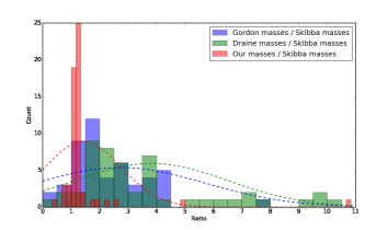
Figure 1.— Ratios of Gordon, Draine and our dust masses to Skibba’s (blue, green and red bars respectively). The dashed blue, green and red lines are gaussian fits of the corresponding histograms. Average dust mass ratios are $Gordon/Skibba$ = 2.73 with $\sigma$ = 2.98, for $Draine/Skibba$ = 3.81 with $\sigma$ = 2.70, and for $ThisWork/Skibba$ = 1.42 with $\sigma$ = 1.34.

2.3. Dust model and extinction law

The amount of extinction depends on wavelength, the dust mass surface density, and the dust model. Extinction can be calculated from

$$\mathrm{A_{\lambda}=[(A_{\lambda}/N_{H})(M_{H}/M_{dust})/m_{H}]\sigma_{dust}},$$ (2)

and the extinction in V is

$A_{V}=[(A_{V}/N_{H})(M_{H}/M_{dust})/m_{H}]\sigma_{dust}$,

where $\sigma_{dust}$ is the dust mass surface density, $N_{H}$ the H column density, $m_{H}$ is the mass of a hydrogen atom, and $A_{V}$/$N_{H}$ is the attenuation per unit column density. The Milky Way $R_{V}$ = 3.1 dust models of Weingartner & Draine (2001) have $A_{V}$/$N_{H}$ = 5.3$\times$10^-22 mag cm² H^-1, and a gas-to-dust mass ratio $M_{H}$/$M_{dust}$ = 98.0392 (see Table 3 in Draine et al. (2007)).

We apply the Cardelli, Clayton, & Mathis (1989) (hereafter CCM) extinction law to calculate the extinction curve:

$$\mathrm{\dfrac{A(\lambda)}{A(V)}=a(x)+b(x)/R_{V}}$$ (3)

where a(x) and b(x) are wavelength dependent coefficients given in CCM.
At infrared wavelengths, 0.3 $\micron^{-1}\leqslant$ x $\leqslant 1.1\micron^{-1}$:

$$\mathrm{a(x)=0.574x^{1.61}}\qquad and\qquad\mathrm{b(x)=-0.527x^{1.61}}$$

and in the visible/NIR, 1.1 $\micron^{-1}\leqslant$ x $\leqslant 3.3\micron^{-1}$:

$$\begin{split}a(x)=1+0.17699y-0.50447y^{2}-0.02427y^{3}+\\ +0.72085y^{4}+0.01979y^{5}-0.77530y^{6}+0.32999y^{7}\end{split}$$

and

$$\begin{split}b(x)=1.4138y+2.28305y^{2}+1.07233y^{3}-5.38434y^{4}+\\ -0.62251y^{5}+5.30260y^{6}-2.09002y^{7}\end{split}$$

where y=(x-1.82) and x=1/$\lambda$.

2.4. Spectral templates of type Ia Supernovae

We use the Hsiao et al. (2007) restframe SNe Ia spectra and light curve templates because they are most complete in temporal and wavelength coverage. The multi-epoch spectral templates range from -20 days before B_max to 80 days after B_max, and were constructed by averaging a large number of observed spectra of nearby SN Ia between 0.1 and 2.5 $\mu$m. We tested the Nugent et al. (2002b) Type Ia Branch-normal templates, and find that they produce similar results.

3. Methods

In this section we describe our Monte Carlo simulation in which we randomly place SNe Ia spectrum templates in KINGFISH galaxies and calculate the dust affected spectrum. The main goal of our Monte Carlo simulation is to create probability plots of SNe Ia color excess as a function of galactocentric distance, and to place uncertainties on the color excess for different galaxy morphology types. We then compare our model to observed spectra of SNe Ia in the KINGFISH galaxies. Finally, we use the generated statistics in the Monte Carlo simulation to determine the absorption-to-reddening ratio $R_{V}$ of dust in host galaxies of a different sample of observed Ia SNe.

3.1. Statistics with KINGFISH sample

To develop color excess statistics we first investigate the relationship between the SNe dust extinction probability and position in the host galaxy. We also look for differences of the effect of dust extinction in galaxies with different morphological classifications. Our procedure was as follows.

The first step was to randomly place the peak brightness template spectrum 100000 times in each of our KINGFISH galaxies, within a radius of 2 $R_{25}$. We assume a peak absolute magnitude $M_{B}$ = -19.5 mag (Saha et al., 1999). The template supernovae are redshifted, and recalculated to observer’s frame using the galaxy distances in Table 2. The random parameters are projected (x,y), centered on the galaxy nucleus, and ext, a parametrization of the extinction, uniformly randomized, corresponding to the fraction of the total amount of dust along the line of sight. A SN in front of the galaxy would have ext = 0, one behind the galaxy ext = 1. For each instance, we calculate $A_{V}$ from equation (2) multiplied by ext, and apply the CCM extinction law with $R_{V}$ = 3.1 to calculate $A_{\lambda}$/$A_{V}$, thus determining the selective extinction with $\lambda$, which, we then subtract from the SN Ia template. In the second step we calculate the observed (B-V) colors, by convolving Bessel B and V filter passbands (Bessell, 1990) with the extincted SN spectrum. The unreddened, intrinsic $(B-V)_{intrinsic}$ = -0.06 mag is calculated from the template spectrum with the same B and V passbands ($A_{V}$ = 0 mag). The outputs are $(B-V)_{observed}$, the color excess $E(B-V)=(B-V)_{observed}-(B-V)_{intrinsic}$, and the projected galactocentric distance in pixels. In Figure 2 we show the distribution of E(B-V) probability with projected $R/R_{25}$ for each galaxy group. E(B-V) peaks near the center, and decreases with radius, as expected, although peak E(B-V) is highest for Sab-Sb types and lowest for S0 and Irregulars.

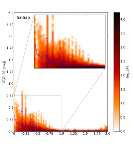
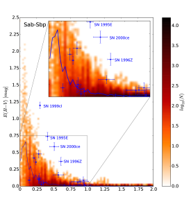
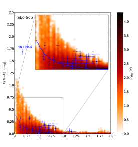
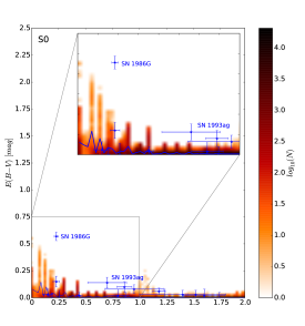
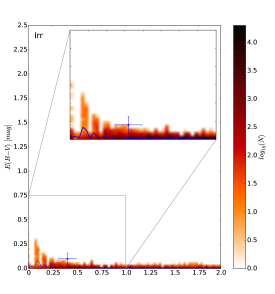
Figure 2.— E(B-V) vs. normalized galactocentric distance probability plots for each of the galaxy groups: Sa-Sap, Sab-Sbp, Sbc-Scp, Scd-Sdm, S0 and Irregulars. The logarithmic color scale indicates the probability that a SN at a certain distance will have a certain color excess E(B-V), dark for high probability, and bright for low probability. The blue crosses indicate observed SNe Ia from the Wang et al. (2006) sample. The blue lines, also shown in the insets and Figure 11, are weighted means of E(B-V) for bins of size 0.025 $R/R_{25}$.

3.2. Comparison with observed SNe Ia in KINGFISH galaxies

There are 15 SNe Ia that occurred in KINGFISH galaxies (Table 3). We found spectra for five SNe in the online Supernova Spectrum Archive (SUSPECT): SN 1981B in NGC 4536, SN 1989B in NGC 3627, SN 2002bo in NGC 3190, SN 2006X in NGC 4321 and SN 1966J in NGC 3198. The spectrum of SN 1966J is digitized from a photographic plate, obtained with the prismatic nebular spectrograph on the Crossley reflector at the Lick Observatory. It is valuable for classification purposes, but as the flux is not properly calibrated (Casebeer et al., 2000) it is not useful for our purpose. The units of the SN 1981B spectra are unknown, and do not agree with commonly used units by Branch (e.g. in Branch et al. (1983, 1981)). General information about SN 1989B, SN2002bo and 2006X are summarized in Table 4.

Having calculated the dust mass in each galaxy pixel, we compare the simulation results to the observed spectra of these historical SNe to see if we can reproduce the observed quantities for $R_{V}$ = 3.1.

The procedure of the comparison is as follows:

1. Match the RA and Dec of the observed SN Ia to the (X,Y) coordinates of the KINGFISH map of the host galaxy.

2. Calculate the extinction curves using $R_{V}$ = 3.1 for different $A_{V}$, from 0 to 3.5 in 0.1 steps

3. $A_{V}$ in the preceeding step are applied to the corresponding restframe template spectra, generating 35 reddened spectra for each epoch.

4. Each spectrum is redshifted into the observer’s frame and the appropriate Milky Way extinction applied.

5. The observed and redshifted templates are convolved with the Subaru intermediate filter passbands (Figure 3, Taniguchi (2004)) in order to have a number of photometric comparison points.

6. To determine $A_{V}$ that best matches the observed spectra we apply the least square test,

   $$\mathrm{\chi^{2}=R^{2}=\sum[OBS_{i}-SIM_{i}]^{2}},$$ (4)

   where $OBS_{i}$ and $SIM_{i}$ are the observed and simulated photometry in the Subaru filters.

7. To calculate E(B-V), the best matching template spectra are convolved with Bessel B and V filter passbands (Bessell (1990), Figure 3) and using $(B-V)_{instrinsic}$ calculated for each epoch.

8. We compare the best fit $A_{V}$, to the calculated $A_{V}$ from the dust assuming ext=1.

9. We also calculate a set of model spectra using different values of $R_{V}$ (from 0.5 to 5.5 in 0.1 steps), which we then compare to the observed spectra as described in steps 2-7. The results are shown in Table 5.

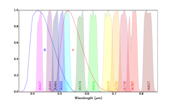
Figure 3.— Subaru Telescope Intermediate Band filters (shaded), and Bessel B (blue line) and V (red line) filters.

Table 3Overview of Ia SNe in the KINGFISH sample

SN	Host galaxy	Mag.	Type	Spectra
SN 1957A	NGC 2841	14.0	Ia-p
SN 1966J	NGC 3198	13.0	Ia	SUSPECT
SN 1980N	NGC 1316	12.5	Ia
SN 1981B	NGC 4536	12.3	Ia	SUSPECT
SN 1989B	NGC 3627	13.0	Ia	SUSPECT
SN 1989M	NGC 4579	12.2	Ia
SN 1994ae	NGC 3370	15.4	Ia
SN 1999by	NGC 2841	15.0	Ia-p
SN 2002bo	NGC 3190	15.5	Ia	SUSPECT
SN 2002cv	NGC 3190	19.0	Ia
SN 2006dd	NGC 1316	15.0	Ia
SN 2006mr	NGC 1316	15.6	Ia
SN 2006X	NGC 4321	17.0	Ia	SUSPECT
SN 2007on	NGC 1404	14.9	Ia
SN 2011iv	NGC 1404	12.8	Ia

Notes. Magnitudes and type were taken from the IAU Central Bureau for Astronomical Telegrams (CBAT) (http://www.cbat.eps.harvard.edu/lists/Supernovae.html).

Table 4General information on SN 1989B, SN2002bo and 2006X

Supernova	Galaxy	Distance	$M_{B}$(max)	$B_{mag}$	$E(B-V)_{Gal}$	Spectra epoch	Spectrum
		$(Mpc)$	$(mag)$	$(mag)$	(mag)	relative to Bmax	references
SN 1989B	NGC 3627	11.07	-19.48	12.34(0.05)	0.032	0, 6, 11, 21, 22, 31, 52	Barbon et al. (1990)
SN 2002bo	NGC 3190	21.6	-19.41	14.06(0.06)	0.027	-4, -3, -1, 4, 28	Benetti et al. (2004)
SN 2006X	NGC 4321	15.2	-19.1	15.41(0.01)	0.026	-6, 0, 2, 6, 8, 12, 13	Yamanaka et al. (2009)

3.2.1 SN 1989B in NGC 3627

SN 1989B is a normal SNe Ia which occurred in a bright spiral arm of NGC 3627, 15”W and 50”N of its nucleus. Figure 4 shows the position of the SN in the dust mass surface density map, compared to optical SDSS and Hubble Space Telescope images. Wells et al. (1994) observed maximum light in B at a magnitude of B = 12.34 $\pm$ 0.05 mag and derived a color excess of E(B-V) = 0.37 $\pm$ 0.03 mag from UBVRIJHK photometry, using Galactic reddening $E(B-V)_{Gal}$ = 0.032 mag, and assuming $R_{V}$ = 3.1 extinction. We simulated the spectra for days 0, 6, 11, 21, 22, 32 and 52, assuming a distance of 11.07 Mpc and an absolute brightness of $M_{B}$(max)=-19.48 mag (Saha et al., 1999). The total dust extinction, calculated from the KINGFISH dust mass column density map of NGC 3627, in V band at the position of SN 1989B is $A_{V}$ = 3.0 mag, in case of ext = 1, when all of dust is taken into account ($\sigma_{dust}$ = 9.667 $\times$10${}^{-5}g$ $cm^{-2}$).

We derive from the simulated best fit spectra E(B-V) = 0.27 $\pm$ 0.07 mag and $A_{V}$ = 0.95 $\pm$ 0.19 mag in case of applying an extinction law with $R_{V}$ = 3.1. Figure 5 shows the best fitted simulated spectrum to the observed spectra (Barbon et al., 1990) at peak brightness. The results are consistent with the Wells et al. (1994) observations. The amount of dust at the location where SN 1989B occurred is enough to cause the observed reddening.

We vary the $R_{V}$ value, and apply the extinction law until the simulated spectrum best fits the observed ones. We derive an average absorption-to-reddening ratio $R_{V}$ = 3.16 $\pm$ 1.54 mag and E(B-V) = 0.34 $\pm$ 0.21 mag from observed spectra at seven different epochs. The results are given in Table 5, and Figure 6 shows of the best fit simulated spectrum to the observed spectra (Barbon et al., 1990) at peak brightness.

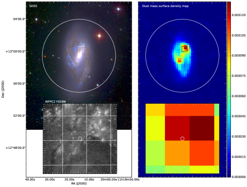
Figure 4.— Top left: Shown is a SDSS gri color image of NGC 3627. The radius of the white circle corresponds to the de Vaucouleur radius $R_{25}$. Bottom left: A Hubble Space Telescope WFPC2/F658N image of the region inside the white box. The small white circle denotes the position of SN 1989B. The radius of 1” corresponds to the position uncertainty. The gird corresponds to pixels of the Herschel’s 500 $\mu$m map. Top right: Dust mass surface density map of NGC 3627. The region inside the black box is shown enlarged bottom right. The white circle denotes the position of the SN, in a high dust density region.

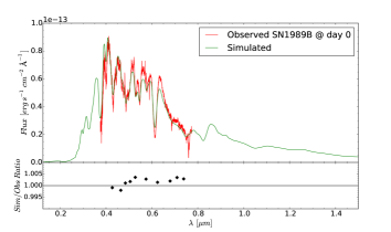
Figure 5.— Comparison between the observed SN 1989B spectrum at peak brightness and the spectral template, for $R_{V}$ = 3.1. The template best matches the observed spectrum after applying CCM extinction law with $A_{V}$ = 1.2 mag. The apparent brightness at maximum light of the simulated best fit spectrum is $m_{B}$ = 12.46 mag, and E(B-V) = 0.37 mag, which is consistent with the observations. The bottom plot shows the ratio between simulated and observed fluxes calculated by convolving the spectra with Subaru Telescope Intermediate Band filters.

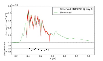
Figure 6.— Comparison between the observed SN 1989B spectrum at peak brightness and the spectral template. The best fit spectrum is obtained by applying the extinction law with $R_{V}$ = 2.2 and $A_{V}$ = 1.1 mag. The apparent brightness at maximum light of the simulated best fit spectrum is $m_{B}$ = 12.48 mag, and E(B-V) = 0.48 mag. The bottom plot shows ratios between simulated and observed fluxes calculated by convolving the spectra with Subaru Telescope Intermediate Band filters.

3.2.2 SN 2002bo in NGC 3190

SN 2002bo is a typical Branch normal SN Ia at visible and infrared wavelengths. Benetti et al. (2004) determined its peak absolute magnitude, $M_{B}$(max) = -19.41 mag, E(B-V) $\sim$ 0.47 mag and a distance of 21.6 Mpc. Milky Way extinction along the line of sight is E(B-V)_Gal = 0.027 mag (Schlegel et al., 1998). The dust mass column density in the KINGFISH dust maps at the position of SN 2002bo, for ext = 1, is $\sigma_{dust}$=(3.155$\pm$0.112)$\times 10^{-5}g$ $cm^{-2}$, corresponding to $A_{V}$ = 0.98 $\pm$ 0.04 mag.

For $R_{V}$ = 3.1, we find that the best fitting template to the observed spectra have $R_{V}$ = 1.34 $\pm$ 0.19 mag and E(B-V) = 0.41 $\pm$ 0.07 mag. This $A_{V}$ value is significantly larger ($\sim$ 35$\%$) than the value calculated from the Herschel derived dust masses. Possible reasons for this discrepancy are:

a) Dust mass uncertainty. Total dust masses for this galaxy range from $10^{6.89}M_{\odot}$ (determined by Skibba) to $10^{7.19}M_{\odot}$ (determined by Draine). Our total integrated mass of $10^{6.97}M_{\odot}$ is $\sim$66$\%$ lower than the Draine et al. (2007) mass, and $\sim$38$\%$ lower than the Gordon (2008) mass, which is sufficient to reach the observed $A_{V}$.

b) $R_{V}\neq$ 3.1. We recalculated the template spectra using values of $R_{V}$ = 0.5 - 5.5 in 0.1 steps, and varying $A_{V}$ between 0 and 3.5 in 0.1 steps for each value of $R_{V}$. We find the best fits to E(B-V) = 0.41 $\pm$ 0.07 mag and $R_{V}$ = 3.24 $\pm$ 0.97, which are consistent with the assumed $R_{V}$ = 3.1. Figure 7 shows a least square colormap for best fit determination of the template to the observed spectra 4 days before peak brightness. Figure 8 shows the observed Benetti et al. (2004) spectra and our best fit computed spectrum for day -1 relative to maximum brightness.

c) Inhomogeneously distributed dust or clumpy dust. At the distance of NGC 3190, a Herschel 500 $\mu$m pixel corresponds to $\sim$1.45 kpc. Figure 9 shows a Hubble Space Telescope ACS/WFC (PropID: 10594) composite image of NGC 3190. SN 2002bo’s position and the 500 $\mu$m SPIRE map pixel are marked. SN 2002bo is inside a spiral arm of NGC 3190 surrounded by clumpy dust features (ACS image); the dust is not smoothly distributed within the SPIRE pixel. If SN 2002bo lies within or behind a dense dust clump, this may explain the larger observed extinction compared to the average $A_{V}$ value calculated for the 500 $\mu$m pixel. The ratio of WFPC2/F336W (PropID: 11966) and ACS-WFC/F814W also shows that the dust is not smoothly distributed near SN 2002bo.

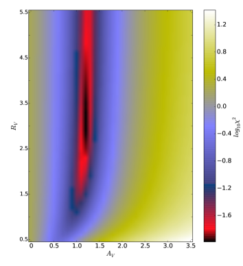
Figure 7.— The distribution of $\chi^{2}$ values for the matching procedure for SN 2002bo, 4 days before peak brightness. We apply an extinction law with a range of different $R_{V}$ and $A_{V}$ values to the spectrum template, and calculate $\chi^{2}$ using observed and simulated Subaru intermediate passbands photometry. In this case, the template best matches the observed spectrum after applying the extinction law with $R_{V}$ = 3.1 and $A_{V}$ = 1.2 mag. However, the difference in $\chi^{2}$ for $R_{V}$ $\sim$ 2.7 - 3.3, at $A_{V}$ = 1.2 mag is very small.

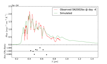
Figure 8.— Comparison between the observed SN 2002bo spectrum 4 days before maximum brightness and the spectral template. The best fit spectrum is obtained by applying extinction law with $R_{V}$ = 3.1 and $A_{V}$ = 1.2 mag. The bottom plot shows ratios between simulated and observed fluxes calculated by convolving the spectra with Subaru Telescope Intermediate Band filters.

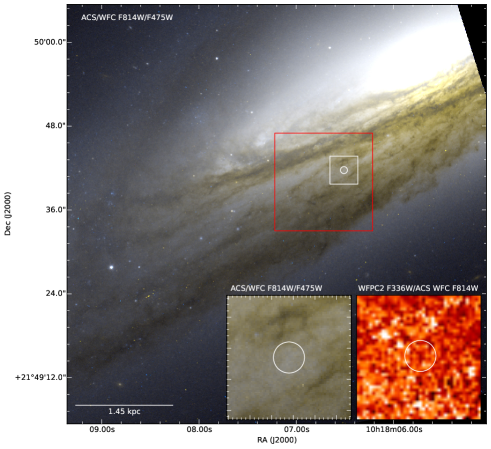
Figure 9.— Hubble Space Telescope ACS/WFC F814W/F475W color image of NGC 3190. The position of SN 2002bo is marked with the small, white circle. The large red square (14” x 14”) is the SPIRE map pixel. The region within the small white box is shown enlarged in the two inset figures, where the r = 0.5” circle corresponds to the position uncertainty of the SN. Bottom left: Zoomed in view of the ACS image. Bottom right: WFPC2 F336W - ACS/WFC F814W color map. In both inset images, the clumpy distribution of dust is noticeable.

3.2.3 SN 2006X in NGC 4321

According to Wang et al. (2008a), SN 2006X is highly reddened by abnormal dust, and compared to other SNe Ia has a peculiar intrinsic color evolution and the highest expansion velocity ever published for a SN Ia. It seems to have a color excess of E(B-V) $\sim$ 1.42 mag with $R_{V}$ $\sim$ 1.48, much smaller than the Milky Way value of $R_{V}$ = 3.1, indicating that the dust surrounding SN 2006X has much smaller grain size than typical interstellar dust. They also note that most of the highly reddened SNe Ia with $E(B-V)_{Host}$ $>$ 0.5, tend to have $R_{V}$ values smaller than 3.1, which suggests that dust surrounding some highly extinguished SNe may be different from that observed in the Galaxy and used in our model. Patat et al. (2009) observed that this SN has high degree of interstellar polarization, peaking in the blue part of the spectrum. Based on Serkowski et al. (1975), Patat et al. (2009) conclude that the dust mixture must be significantly different from typical Milky Way dust, with a lower total to selective extinction ratio $R_{V}$ than commonly measured in the Milky Way. They suggest that the bulk of the extinction is due to a molecular cloud.

We used the Cepheid distance to NGC 4321 of 15.2 Mpc, and an absolute brightness at peak of $M_{B}$ = -19.1 mag (Wang et al., 2008b) to best fit the simulated spectra to observations. At the position of SN 2006X in the extinction map of NGC 4321, $A_{V}$ = 1.05 mag (for $R_{V}$= 3.1), and, Milky Way reddening along the line of sight is $E(B-V)_{Gal}$ = 0.026 mag. We determined from spectra at seven different epochs (Table 5) an average $R_{V}$ = 1.46 $\pm$ 0.29, and E(B-V) = 1.39 $\pm$ 0.05 mag. This $R_{V}$ ratio is consistent with the values determined by others. The observed spectra of SN 2006X do not fit the computed extinguished spectra with $R_{V}$ = 3.1 dust (Figure 10).

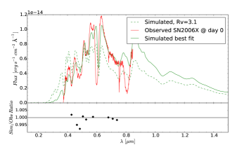
Figure 10.— Comparison of template spectra and the observed spectrum of SN 2006X at peak brightness. The dashed line is the best fit template with $R_{V}$ = 3.1, and $A_{V}=2.4$ mag. The solid green line is the best fit for an extinction law with $R_{V}$ = 1.6 and $A_{V}$ = 2.2 mag.

Table 5KINGFISH SNe best fit results. The range is: 0.5 $>R_{V}>$5.5; 0.0$>A_{V}>$3.5, step size=0.1

		Best fit					Fixed $R_{V}$=3.1
SN name	$Epoch$	$R_{V}$	$A_{V}$	$E(B-V)_{Host}$	$B_{mag}$	$B-V$	$A_{V}$	$E(B-V)_{Host}$	$B_{mag}$	$B-V$
	$(day)$		(mag)	(mag)	$(mag)$	(mag)	(mag)	(mag)	(mag)	(mag)
SN 1989B	0	2.2	1.1	0.48	12.48	0.48	1.2	0.37	12.46	0.37
	6	2.5	1.0	0.37	12.47	0.51	1.0	0.29	12.39	0.44
	11	1.1	0.9	0.75	13.18	1.07	1.1	0.32	12.93	0.64
	21	2.9	1.1	0.32	14.03	1.17	1.1	0.30	14.0	1.15
	22	5.4	0.9	0.13	13.73	1.04	0.9	0.24	13.85	1.15
	32	5.5	0.7	0.09	14.26	1.20	0.6	0.15	14.22	1.26
	52	2.5	0.8	0.27	15.17	1.19	0.8	0.21	15.11	1.13
SN 2002bo	-4	3.1	1.2	0.37	14.09	0.29	1.2	0.37	14.09	0.29
	-3	3.0	1.2	0.39	14.04	0.33	1.2	0.37	14.03	0.31
	-1	2.3	1.2	0.51	14.11	0.48	1.3	0.41	14.10	0.38
	4	2.7	1.3	0.46	14.25	0.54	1.3	0.40	14.18	0.48
	28	5.1	1.8	0.31	16.83	1.43	1.7	0.47	16.9	1.59
SN 2006X	-6	1.4	2.0	1.37	15.66	1.29	2.2	0.70	15.17	0.62
	0	1.6	2.2	1.31	15.46	1.30	2.4	0.76	15.10	0.75
	2	0.9	1.4	1.45	14.83	1.48	1.7	0.53	14.19	0.56
	6	1.4	2.1	1.39	15.64	1.52	2.3	0.71	15.15	0.84
	8	1.8	2.7	1.38	16.37	1.57	2.8	0.86	15.94	1.05
	12	1.3	2.2	1.49	16.37	1.84	2.5	0.75	15.91	1.10
	13	1.8	2.8	1.37	16.95	1.76	3.0	0.88	16.65	1.28

4. Results & discussion

4.1. Color excess probabilities

As described in $\S$2.1, we divided the galaxies into six groups according to their morphology. For each group, we binned the color excess values and galactocentric distances from the Monte Carlo simulation in bins of 0.025 mag for E(B-V) and 0.025 for normalized galactrocenric distances $R/R_{25}$. The color excess probability maps are shown in Figure 2. The color indicates the number of Ia SNe with a certain E(B-V) value at a certain distance from the galaxy center. The variation in dust mass distribution and amount among galaxy types affects the color excess E(B-V). From our simulation, we expect that the most extinguished SNe will occur in Sab-Sb galaxies, the most dust rich galaxy class, while SNe in S0 and Irregulars are less affected by dust. The blue lines are the mean, i.e. most probable, E(B-V). The blue crosses are observed SNe Ia from Wang et al. (2006) (Table 1 and 2).

We fit the mean color excess values as a function of $R/R_{25}$:

$$\mathrm{E_{B-V}(R/R_{25})=\textit{f}(R/R_{25})=a\exp(b(R/R_{25})^{c})},$$ (5)

where a, b and c are free parameters determined by the least square method. Figure 11 compares the mean E(B-V) to the fitted functions. The parameters and standard deviations for different galaxy types are given in Table 6. The most probable extinction $A_{V}$ can be derived from the color excess functions simply by multiplying by 3.1.

In $\S$3.2 we compared the observed spectra of three individual SNe Ia in three KINGFISH galaxies to our model where we assume a dust model with $R_{V}$ = 3.1 and uniformly distributed dust along the line of sight in the host galaxy. The color excess then depends on the depth of the supernova into the galaxy, which we take as a free random parameter (ext). For each position there is therefore a range of possible E(B-V) values constrained by an upper limit.

To test the reliability of our Monte Carlo simulation, we compared our calculated upper limits of E(B-V) as a a function of galactocentric distance for different morphological galaxy classes to the observed E(B-V) values of a larger sample of 109 low redshift ($\lesssim$ 0.1) SNe Ia, collected by Wang et al. (2006), for which they determined the reddening distribution of SNe in their respective host galaxies (Figure 2).

The color excess of all 7 SNe in Sa-Sap galaxies and 1 SN in an Irregular galaxy is lower than the upper E(B-V) limit in our Monte Carlo simulation, consistent with the simulation.

In Sab-Sbp galaxies, 4 of 21 observed SNe (SN 1999cl, SN 1995E, SN 2000ce and SN 1996Z) have $\sim$0.1-0.25 mag higher E(B-V) than our simulation’s upper limit. In the case of SN 1999cl, Krisciunas et al. (2006) and Wang et al. (2006) find $R_{V}\approx$ 1.5, indicating nonstandard dust that explains the offset.

Of the 34 SNe Ia in Sbc-Scp galaxies, only SN 1996ai is highly reddened, and whose observed E(B-V) = 1.69 $\pm$ 0.06 mag is about $\sim$0.7 mag redder than our model upper limit.

In Scd-Sdm galaxies, one of the 7 observed SNe is inconsistent with the simulation result. SN 1997br is a spectroscopically peculiar SN 1991T-like supernova, whose E(B-V) is $\sim$0.2 mag higher than the highest possible expected value in our model. Wang et al. (2006) suggest that SN 1997br’s host galaxy dust is very different from typical Milky Way dust, which may explain the inconsistency.

Finally, only 2 of 17 SNe Ia in S0 galaxies have larger reddening than expected from our Monte Carlo simulations. SN 1986G’s value of E(B-V) is about 0.25 mag higher than the maximum expected value, and SN 1993ag, has an observed E(B-V) $\sim$ 0.1 mag, slightly larger than the upper limit.

In total, $\sim$91$\%$ of observed SNe have a smaller color excess than the upper limit of E(B-V) in Monte Carlo, implying that our model’s amount of dust is in most cases sufficient to produce the observed color excess. The remaining 9$\%$ SNe have larger observed color excess compared to the expected model upper limit because our model underestimates either the amount of dust, or $R_{V}$ $<3.1$ (e.g. SN 1999cl, SN 1997br, SN 2006X), or more likely, there is a local dust overdensity in front of the SNe (e.g. SN 2002bo).

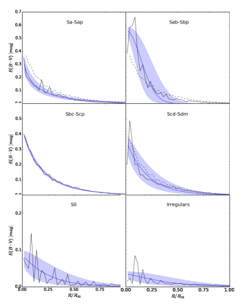
Figure 11.— Mean E(B-V) values from our Monte Carlo simulation (black line) compared to the fitted $E_{B-V}(R/R_{25})$ functions (eq.5, blue line) for different morphological classes. The shaded blue shows the 1-$\sigma$ uncertainty of the best fit parameters (Table 6). The dashed line in the late-type galaxies panels is the mean E(B-V) value for the Sbc-Scp galaxies group, plotted for comparison reasons.

Table 6Color excess function parameters

	$E_{B-V}(R/R_{25})=a\exp(b(R/R_{25})^{c})$
Galaxy type	$a$	$b$	$c$
Sa-Sap	0.43(0.04)	-3.87(0.16)	0.59(0.05)
Sab-Sbp	0.56(0.03)	-24.91(9.98)	2.02(0.28)
Sbc-Scp	0.45(0.01)	-4.1(0.07)	0.85(0.02)
Scd-Sdm	0.36(0.04)	-4.98(0.8)	1.00(0.16)
S0	0.08(0.01)	-4.6(1.36)	1.11(0.32)
Irregular	0.03(0.01)	-3.34(1.07)	1.30(0.48)

4.2. Estimating $R_{V}$ of SNe Ia host galaxy dust

In section 4.1, we showed that starting with integrated dust mass values and $R_{V}$ = 3.1, we can calculate $A_{V}$ and determine the most likely value of E(B-V). In this section we invert the process to determine the most likely absorption-to-reddening ratio $R_{V}$, given E(B-V).

From the statistical sample of color excesses $E(B-V)_{SIM}$ as a function of galactocentric distance generated by the Monte Carlo simulation, we estimate the $R_{V}$ for host galaxy dust of the Wang et al. (2006) sample. We grouped these SNe by host galaxy morphology as per the KINGFISH galaxies, resulting in 7, 21, 34, 7, 17 and 1 galaxies classified as Sa-Sap, Sab-Sbp, Sbc-Scp, Scd-Sdm, S0 and Irregulars respectively.

The color excess E(B-V) = $A_{V}$/$R_{V}$ is measured by assuming an intrinsic SNe brightness and a distance. $A_{V}$ depends on the dust column density and $R_{V}$ on the physical properties of dust.

If we now assume that the most probable color excess caused by dust extinction in galaxies can be described with functions given in Table 6, for a fixed extinction $A_{V}$, i.e. fixed dust amount, varying $R_{V}$ changes the color excess E(B-V). Thus, we use the least square method to determine a factor at which our functions of most probable color excess (Table 6) best fit the Wang et al. (2006) sample. We then estimate the $R_{V}$ of the sample by dividing 3.1 with the determined factor.

Wang et al. (2006) calculated host galaxy reddening by averaging E(B-V) determined from the (B-V) color curve at late times (cf. Lira, 1995) and E(B-V) determined from (B-V) 12 days after maximum, $\Delta C_{12}$. SNe absolute V magnitudes were then calculated as a function of $\Delta C_{12}$, and plotted against E(B-V) of the host galaxies. The slope is $R_{V}$. They derive $R_{V}$ = 2.30 $\pm$ 0.11, and suggest that the remarkably small scatter indicates that the dust properties are similar in z $\lesssim$ 0.1 host galaxies.

We use our reddening statistics to estimate the $R_{V}$ value for the Wang et al. (2006) subsamples of 21 Ia SNe observed in Sab-Sbp galaxies, and 34 SNe in Sbc-Scp. We find that our function of galactocentric distance for most probable color excess E(B-V) best matches the sample of observed SNe in Sab-Sbp galaxies if multiplied with 1.14 $\pm$ 0.67 (Figure 12), which corresponds to $R_{V}$ = 2.71 $\pm$ 1.58. In the case of SNe in Sbc-Scp galaxies, we find $R_{V}$ = 1.70 $\pm$ 0.38 (Figure 13). Both $R_{V}$ values are smaller than the common ratio for Milky way dust, which is consistent with the recent earlier studies (see Table 1). This method of $R_{V}$ estimation requires a large sample of observed SNe. The subsample of 7, 7, 17 and 1 observed SNe in Sa-Sap, Scd-Sdm, S0 and Irregulars respectively, is not enough to get a reasonable result.

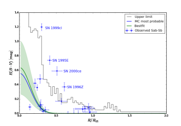
Figure 12.— Blue crosses show a sample of 21 Ia SNe in Sab-Sbp galaxies. The sample best matches the function of most probable color excess for SNe Ia in Sab-Sbp galaxies (blue line) if multiplied by 1.14 $\pm$ 0.67 (green line). The shaded green is the 1-$\sigma$ uncertainty.

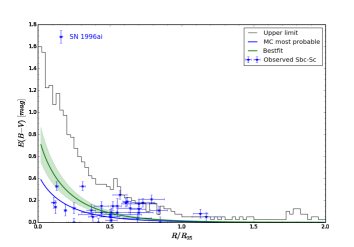
Figure 13.— Blue crosses show a sample of 34 Ia SNe in Sbc-Scp galaxies from Wang et al. (2006). The sample best matches the function of most probable color excess for SNe Ia in Sbc-Scp galaxies (blue line) if multiplied by 1.82 $\pm$ 0.41 (green line). The shaded green is the 1-$\sigma$ uncertainty.

4.3. Model uncertainty and effect on results

The main uncertainty which can significantly affect the results is the systematic uncertainty of dust masses. Our integrated dust masses are consistent with the masses calculated by Skibba et al. (2011), but there is a discrepancy with dust masses determined by Draine et al. (2007) and Gordon (2008), who use different methods. Gordon (2008) estimated the masses from 70 $\mu$m to 160 $\mu$m flux ratio, assuming the dust radiates as a black body with emissivity $\propto\lambda^{-2}$, a simple dust model consisting of 0.1 $\mu$m silicon grains. Draine et al. (2007) calculated the masses by fitting a multicomponent dust model to the galaxy spectral energy distribution.

For each galaxy in our sample (Table 2) we computed dust mass ratios of the Draine, Gordon and Skibba values. The distribution is shown in Figure 1. Our dust masses, are in average 2.02 $\pm$ 1.07 and 3.12 $\pm$ 2.24 times lower than the masses derived using Karl Gordon’s dust mass maps, and the masses determined by Draine et al. (2007) respectively. The median of the ratios of Gordon’s to our, and Draine’s to our masses are 1.8, and 2.4 respectively. The discrepancy in the dust mass may be caused by different dust temperature estimates, dust models, but are also correlated with the distance to the galaxies. We used distances given in Skibba et al. (2011) which they took from Kennicutt et al. (2011), while Draine et al. (2007) use distances from Kennicutt et al. (2003). Calculating the dust masses with distances from Kennicutt et al. (2003) give us 2.7 $\pm$ 1.3, and 1.8 $\pm$ 0.7 times lower masses from Draine et al. (2007) and Gordon respectively. The dust mass ratios are summarized in Table 7.

The total dust mass is linearly related to $A_{V}$ and E(B-V), and thus the color excess functions given in Table 6. If there would hypothetically be twice as much dust in our model, the color excess would be twice as large, and the estimated $R_{V}$ ratios would be larger; $R_{V}$ = 3.40 $\pm$ 0.76 for Sab-Sb, and $R_{V}$ = 5.42 $\pm$ 3.16 for Sbc-Sc.

Table 7Dust mass ratio comparison

Distances	Skibba et al. (2011)		Kennicutt et al. (2003)
Ratio	Mean	Median	Mean	Median
Our/Skibba	1.43(1.35)	1.18	1.54(1.38)	1.20
Draine/Skibba	3.81(2.70)	2.73	…	…
Gordon/Skibba	2.73(2.98)	1.97	…	…
Draine/Our	3.12(2.24)	2.35	2.73(1.31)	2.46
Gordon/Our	2.02(1.07)	1.82	1.82(0.72)	1.74

4.4. Effects of circumstellar dust

In this work we assume that extinction is produced only by dust in the SN host galaxy’s ISM, although there is evidence that circumstellar material (CSM), ejected by the progenitor system, may contribute to normal SNe Ia reddening.

Patat et al. (2007) performed high resolution spectroscopy of the highly reddened SN 2006X from five different epochs and observed clear time evolution of the Na I D doublet lines. They suggest that the evolution is caused by changes in CSM ionization conditions induced by the variable SN radiation field. They calculated the Na I column density from the most intense feature at day +14, N(Na I) $\cong$ $10^{12}$ $cm^{-2}$. For comparison, we calculated the extinction $A_{V}\approx$ 0.001 mag, assuming the solar Na abundance, log Na/H = -6.3, and the attenuation per unit column density for standard interstellar dust as used in our model, $A_{V}/N_{H}$ = 5.3$\times$ 10^-22 mag cm² H^-1 (Draine & Li, 2007).

Blondin et al. (2009) analyzed low resolution, high signal to noise spectra of 294 SNe Ia obtained by the CfA Supernova Program, and were able to measure changes in the equivalent width of the NaI lines in two SNe: SN 1999cl and SN 2006X. The deduced Na I column density is log N(Na I) $\approx$ 14.3, corresponding to $A_{V}\approx$ 0.21 mag, assuming the (Draine & Li, 2007) dust model and solar Na abundance. Like SN 2006X, SN 1999cl is also highly reddened: E(B-V) $\approx$ 1.2, $R_{V}\approx$ 1.6. This detection of variable Na I D features in two of the most reddened SNe suggests that the change in EW with time might be associated with circumstellar or interstellar absorption (Blondin et al., 2009). However, no such variation is detected in the highly reddened SN 2003cg (E(B-V) $\approx$ 1.3 mag, $R_{V}\approx$ 1.8) (Elias-Rosa et al., 2006).

Wang et al. (2007) found a strong correlation between polarization across the Si II line and $\bigtriangleup m_{15}$, possibly indicative of large-scale asymmetries, such as large plumes located above the SN photosphere, or generated from the interaction of the ejecta with circumstellar material, such as an accretion disk before the explosion of the white dwarf progenitor.

Johansson et al. (2013) used Herschel PACS 70 $\mu$m observations of three nearby SNe Ia to search for pre-existing circumstellar dust. They derive upper limits on CS dust masses based on nondetection. Assuming 0.1 $\mu$m graphitic or silicate dust grains in a pre-existing dust shell with radius $r_{d}$ $\sim$ 10¹⁷ cm (cf. Patat et al. (2007)), heated to $T_{d}$ $\sim$ 500 K, they obtained $M_{d}\leq$ 7 $\times$ 10^-3 M_⊙ for SN 2011fe, and $M_{d}$ $<$ 10^-1 $M_{\odot}$ for SNe 2011by and 2012cg. Assuming that the dust is distributed in a dust shell of $r_{d}\sim$ 10¹⁷ cm, we can exclude dust mass surface densities $\sigma_{dust}$ $>$ 10^-4 g/cm² and $\sigma_{dust}\gtrsim$ 1.6 $\times$ 10^-3 g/cm² for SN 2011fe and for SNe 2011by and 2012cg respectively. Those upper limits are still at least an order of magnitude larger than the dust mass surface densities required to produce significant extinction, so that it can not be ruled out that there is CSM, which affects the colors Ia SNe.

At present, the available studies can neither definitely exclude SNe Ia reddening by circumestellar dust nor affirm that CSM dust is responsible for the low $R_{V}$ values.

5. Summary

• We use dust temperature estimations by Skibba et al. (2011) and Herschel 500 $\mu$m SPIRE maps to create pixel-by-pixel dust mass surface density maps for a sample of 59 KINGFISH galaxies (Kennicutt et al., 2011).

• Comparison of our model to SN 1989B, SN 2002bo and SN 2006X, three individual SNe Ia which occurred in KINGFISH galaxies, shows that our model is in good agreement with the observations. We are able explain and reproduce the observed spectra.

• We grouped the KINGFISH sample into six galaxy groups according to the morphology, and ran Monte Carlo simulations to place constrains on the color excess as a function of galactocentric distance. We developed a color excess probability model due to dust extinction and show the differences between galaxy groups. We find that the largest reddening probability is expected in Sab-Sbp and Sbc-Sc galaxies, while S0 and Irregulars are very dust poor. We determine the most probable reddening for different galaxy classes as a function of $R/R_{25}$ (Table 6). The functions can be used to estimate reddening of SNe Ia depending on the host galaxy morphology and the galactocentric distance of the observed SNe, or for extinction correction studies for Type Ia supernova rates (e.g. Riello & Patat (2005)).

• We present a new approach for determination of the absorption-to-reddening ratio $R_{V}$ using statistics of color excess developed in a Monte Carlo simulation. We find for a sample of 21 Ia SNe observed in Sab-Sbp galaxies, and 34 SNe in Sbc-Scp, an $R_{V}$ of 2.71 $\pm$ 1.58 and $R_{V}$ = 1.70 $\pm$ 0.38 respectively, but the results strongly depend on the derived values for dust mass.

References

- Altavilla et al. (2004) Altavilla, G., Fiorentino, G., Marconi, M., et al. 2004, MNRAS, 349, 1344
- Barbon et al. (1990) Barbon, R., Benetti, S., Rosino, L., Cappellaro, E., & Turatto, M. 1990, A&A, 237, 79
- Benetti et al. (2004) Benetti, S., Meikle, P., Stehle, M., et al. 2004, MNRAS, 348, 261
- Bessell (1990) Bessell, M. S. 1990, PASP, 102, 1181
- Blondin et al. (2009) Blondin, S., Prieto, J. L., Patat, F., et al. 2009, ApJ, 693, 207
- Branch et al. (1981) Branch, D., Falk, S. W., Uomoto, A. K., et al. 1981, ApJ, 244, 780
- Branch et al. (1983) Branch, D., Lacy, C. H., McCall, M. L., et al. 1983, ApJ, 270, 123
- Branch & Tammann (1992) Branch, D., & Tammann, G. A. 1992, ARA&A, 30, 359
- Buta et al. (2010) Buta, R. J., Sheth, K., Regan, M., et al. 2010, ApJS, 190, 147
- Cardelli et al. (1989) Cardelli, J. A., Clayton, G. C., & Mathis, J. S. 1989, ApJ, 345, 245
- Casebeer et al. (2000) Casebeer, D., Branch, D., Blaylock, M., et al. 2000, PASP, 112, 1433
- Conley et al. (2007) Conley, A., Carlberg, R. G., Guy, J., et al. 2007, ApJ, 664, L13
- de Vaucouleurs et al. (1991) de Vaucouleurs, G., de Vaucouleurs, A., Corwin, Jr., H. G., et al. 1991, Third Reference Catalogue of Bright Galaxies. Volume I: Explanations and references. Volume II: Data for galaxies between 0h and 12h. Volume III: Data for galaxies between 12h and 24h.
- Draine (2003a) Draine, B. T. 2003a, ARA&A, 41, 241
- Draine (2003b) —. 2003b, ApJ, 598, 1026
- Draine & Li (2007) Draine, B. T., & Li, A. 2007, ApJ, 657, 810
- Draine et al. (2007) Draine, B. T., Dale, D. A., Bendo, G., et al. 2007, ApJ, 663, 866
- Elias-Rosa et al. (2006) Elias-Rosa, N., Benetti, S., Cappellaro, E., et al. 2006, MNRAS, 369, 1880
- Folatelli et al. (2010) Folatelli, G., Phillips, M. M., Burns, C. R., et al. 2010, AJ, 139, 120
- Goobar (2008) Goobar, A. 2008, ApJ, 686, L103
- Gordon (2008) Gordon, K. 2008, personal communication
- Gordon et al. (2010) Gordon, K. D., Galliano, F., Hony, S., et al. 2010, A&A, 518, L89
- Hicken et al. (2009a) Hicken, M., Wood-Vasey, W. M., Blondin, S., et al. 2009a, ApJ, 700, 1097
- Hicken et al. (2009b) Hicken, M., Challis, P., Jha, S., et al. 2009b, ApJ, 700, 331
- Hsiao et al. (2007) Hsiao, E. Y., Conley, A., Howell, D. A., et al. 2007, ApJ, 663, 1187
- Johansson et al. (2013) Johansson, J., Amanullah, R., & Goobar, A. 2013, MNRAS, 431, L43
- Kennicutt et al. (2011) Kennicutt, R. C., Calzetti, D., Aniano, G., et al. 2011, PASP, 123, 1347
- Kennicutt et al. (2003) Kennicutt, Jr., R. C., Armus, L., Bendo, G., et al. 2003, PASP, 115, 928
- Kessler et al. (2009) Kessler, R., Becker, A. C., Cinabro, D., et al. 2009, ApJS, 185, 32
- Kowalski et al. (2008) Kowalski, M., Rubin, D., Aldering, G., et al. 2008, ApJ, 686, 749
- Krisciunas et al. (2006) Krisciunas, K., Prieto, J. L., Garnavich, P. M., et al. 2006, AJ, 131, 1639
- Lampeitl et al. (2010) Lampeitl, H., Smith, M., Nichol, R. C., et al. 2010, ApJ, 722, 566
- Lira (1995) Lira, P. 1995, Master’s thesis, University of Chile, Chile
- Mandel et al. (2011) Mandel, K. S., Narayan, G., & Kirshner, R. P. 2011, ApJ, 731, 120
- Miller & Branch (1990) Miller, D. L., & Branch, D. 1990, AJ, 100, 530
- Nobili & Goobar (2008) Nobili, S., & Goobar, A. 2008, A&A, 487, 19
- Nobili et al. (2003) Nobili, S., Goobar, A., Knop, R., & Nugent, P. 2003, A&A, 404, 901
- Nugent et al. (2002a) Nugent, P., Kim, A., & Perlmutter, S. 2002a, PASP, 114, 803
- Nugent et al. (2002b) —. 2002b, PASP, 114, 803
- Patat et al. (2009) Patat, F., Baade, D., Höflich, P., et al. 2009, A&A, 508, 229
- Patat et al. (2007) Patat, F., Chandra, P., Chevalier, R., et al. 2007, Science, 317, 924
- Perlmutter et al. (1999) Perlmutter, S., Aldering, G., Goldhaber, G., et al. 1999, ApJ, 517, 565
- Phillips (1993) Phillips, M. M. 1993, ApJ, 413, L105
- Phillips et al. (1999) Phillips, M. M., Lira, P., Suntzeff, N. B., et al. 1999, AJ, 118, 1766
- Reindl et al. (2005) Reindl, B., Tammann, G. A., Sandage, A., & Saha, A. 2005, ApJ, 624, 532
- Riello & Patat (2005) Riello, M., & Patat, F. 2005, MNRAS, 362, 671
- Riess et al. (1996a) Riess, A. G., Press, W. H., & Kirshner, R. P. 1996a, ApJ, 473, 88
- Riess et al. (1996b) —. 1996b, ApJ, 473, 588
- Riess et al. (1998) Riess, A. G., Filippenko, A. V., Challis, P., et al. 1998, AJ, 116, 1009
- Saha et al. (1999) Saha, A., Sandage, A., Tammann, G. A., et al. 1999, ApJ, 522, 802
- Schlegel et al. (1998) Schlegel, D. J., Finkbeiner, D. P., & Davis, M. 1998, ApJ, 500, 525
- Serkowski et al. (1975) Serkowski, K., Mathewson, D. S., & Ford, V. L. 1975, ApJ, 196, 261
- Skibba et al. (2011) Skibba, R. A., Engelbracht, C. W., Dale, D., et al. 2011, ApJ, 738, 89
- Sullivan et al. (2006) Sullivan, M., Le Borgne, D., Pritchet, C. J., et al. 2006, ApJ, 648, 868
- Taniguchi (2004) Taniguchi, Y. 2004, in Studies of Galaxies in the Young Universe with New Generation Telescope, ed. N. Arimoto & W. J. Duschl, 107–111
- Wang (2005) Wang, L. 2005, ApJ, 635, L33
- Wang et al. (2007) Wang, L., Baade, D., & Patat, F. 2007, Science, 315, 212
- Wang et al. (2008a) Wang, X., Li, W., Filippenko, A. V., et al. 2008a, ApJ, 677, 1060
- Wang et al. (2006) Wang, X., Wang, L., Pain, R., Zhou, X., & Li, Z. 2006, ApJ, 645, 488
- Wang et al. (2008b) Wang, X., Li, W., Filippenko, A. V., et al. 2008b, ApJ, 675, 626
- Weingartner & Draine (2001) Weingartner, J. C., & Draine, B. T. 2001, ApJ, 548, 296
- Wells et al. (1994) Wells, L. A., Phillips, M. M., Suntzeff, B., et al. 1994, AJ, 108, 2233
- Yamanaka et al. (2009) Yamanaka, M., Naito, H., Kinugasa, K., et al. 2009, PASJ, 61, 713