Asymmetric interiors for small black holes

Daniel Kabat¹, Gilad Lifschytz²

¹Department of Physics and Astronomy

Lehman College, City University of New York, Bronx NY 10468, USA

²Department of Mathematics

Faculty of Natural Science, University of Haifa, Haifa 31905, Israel

We develop the representation of infalling observers and bulk fields in the CFT as a way to understand the black hole interior in AdS. We first discuss properties of CFT states which are dual to black holes. We then show that in the presence of a Killing horizon bulk fields can be decomposed into pieces we call ingoing and outgoing. The ingoing field admits a simple operator representation in the CFT, even inside a small black hole at late times, which leads to a simple CFT description of infalling geodesics. This means classical infalling observers will experience the classical geometry in the interior. The outgoing piece of the field is more subtle. In an eternal two-sided geometry it can be represented as an operator on the left CFT. In a stable one-sided geometry it can be described using entanglement via the PR construction. But in an evaporating black hole trans-horizon entanglement breaks down at the Page time, which means that for old black holes the PR construction fails and the outgoing field does not see local geometry. This picture of the interior allows the CFT to reconcile unitary Hawking evaporation with the classical experience of infalling observers.

1 Introduction

Black holes provide an ideal theoretical laboratory for testing attempts to reconcile gravity with quantum mechanics. There is a basic tension between the semiclassical geometry thought to describe an evaporating black hole, shown in Fig. 1, and the requirement of unitary time evolution. For a survey including recent developments see [1].

Figure 1: An evaporating AdS-Schwarzschild black hole, formed by a null shell sent in from the boundary. The semiclassical geometry suggests that an infalling object will hit the singularity and be lost to the outside world, while unitary time evolution requires the pure states $|i\rangle$ and $|f\rangle$ to be related by a unitary transformation.

In this paper we assume that AdS/CFT provides a complete description of quantum gravity in asymptotically AdS space. This guarantees unitary time evolution for the underlying CFT degrees of freedom but leads one to question the meaning of space-time inside the horizon. We probe this region by attempting to represent local bulk fields in the black hole interior in terms of the CFT. For bulk points outside the horizon the representation of a bulk field in terms of the CFT is well-understood: in the $1/N$ expansion one can define CFT operators which mimic local bulk fields when inserted in correlation functions. This has been developed for free scalar fields [2, 3, 4, 5, 6, 7] and free fields with spin [8, 9, 10], and in empty AdS follows from representation theory [11, 12]. Perturbative $1/N$ corrections have been studied in [13, 14, 15, 16, 17]. For other approaches see [18, 19, 20].

But inside a black hole with finite entropy (and a single asymptotic region) it seems unlikely that bulk fields directly correspond to CFT operators [21]. Given this, does the space-time region inside the horizon have any meaning? We will argue that it does, in the sense that even for evaporating black holes the CFT accurately describes the geometry seen by an infalling classical observer.

To show this we start from the simple observation that in the presence of a horizon a bulk field can be decomposed into parts we call ingoing and outgoing. This decomposition is crucial because, as we will see, the CFT treats these two parts of the field very differently. Outside the horizon both parts can be represented as operators in the CFT. But inside the horizon only the ingoing part of the field has a straightforward representation as an operator in the CFT. The outgoing piece does not have such a representation. Fortunately Papadodimas and Raju (PR) [22, 23, 24] proposed a different method for representing fields in the interior which can be used to express the outgoing field in the CFT. The PR construction depends on entanglement across the horizon. Given the maximal pairwise entanglement expected from supergravity, and the known representation of local operators outside the horizon, one can write CFT operators which act as local fields on the entangled partners in the interior.

The PR construction can be applied to an evaporating black hole, but there is a subtlety. Unitarity of the CFT and monogamy of entanglement imply that after the Page time outgoing Hawking particles are entangled, not with the black hole interior, but rather with the distant early Hawking radiation. Once pairwise trans-horizon entanglement is lost the PR construction cannot be used to write local operators in the interior. It seems that after the Page time there is no way to recover conventional space-time geometry in the interior from the CFT. Indeed it’s been argued that a firewall forms at the Page time [25].

Here we argue for a different outcome. In classical gravity one way to show that the interior exists is to note that infalling geodesics do not stop at the horizon but rather continue all the way to the singularity. We wish to make a similar argument in AdS/CFT. To do this we construct bulk wavepackets which track infalling geodesics. We show that such wavepackets can be constructed using only the infalling part of the field, which is the part that can be represented in the CFT. These wavepackets track geodesics which cross the horizon and continue all the way to the singularity. This is true even after the Page time!

So evaporating black holes do have an interior space-time geometry, in the restricted sense that the CFT can describe classical objects falling into the black hole. Although classical infall may be geometric, for the outgoing part of the field the notion of interior geometry breaks down at the Page time. So the CFT predicts no drama for infalling observers, while simultaneously realizing the partial breakdown of geometry that is required for unitary evaporation.

In the rest of the paper we elaborate on these statements. Since the bulk of the paper is somewhat lengthy, we provide below an overview of our approach. Up to this point we have emphasized evaporating black holes, but from here on we allow for more general possibilities.

*                        *                        *

We start in section 2 by discussing properties of CFT states which are dual to black holes. In particular we discuss the formation and evaporation of a black hole in the context of the eigenstate thermalization hypothesis, contrasting the behavior of stable and evaporating black holes. Although the discussion in this section is not strictly necessary for the rest of the paper, it provides an important context for what follows.

In section 3 we make the simple observation that in the presence of a horizon a field can be decomposed into “ingoing” and “outgoing” modes. This is just the well-known fact that in terms of a tortoise coordinate $r_{*}$, in the near-horizon region modes have two possible behaviors.

$${\rm ingoing:}\qquad\phi\sim e^{-i\omega(t+r_{*})}$$ (1)

$${\rm outgoing:}\qquad\phi\sim e^{-i\omega(t-r_{*})}$$

Note that ingoing modes are smooth across the future horizon while outgoing modes are singular. The reason for this behavior is that we’re diagonalizing a Killing vector which is null on the horizon.

Perhaps not surprisingly, the ingoing part of the field has a simple representation as an operator in the CFT, even for bulk points inside the horizon. We work out examples of these CFT operators in section 4 for AdS₂ in Rindler coordinates and in section 5 for AdS₃ and BTZ black holes. The simplest case is a free massless scalar field in AdS₂, for which the ingoing and outgoing parts of the field can be represented in terms of an operator ${\cal O}$ in the CFT by

$$\phi_{\rm in}(t,r_{*})={1\over 2R^{2}}\int_{t+r_{*}}^{\infty}dt^{\prime}\,{\cal O}(t^{\prime})$$ (2)

$$\phi_{\rm out}(t,r_{*})=-{1\over 2R^{2}}\int_{t-r_{*}}^{\infty}dt^{\prime}\,{\cal O}(t^{\prime})$$

Outside the horizon both $\phi_{\rm in}$ and $\phi_{\rm out}$ are well-defined and one recovers the full bulk field from the combination $\phi_{\rm in}+\phi_{\rm out}$. But as a CFT operator $\phi_{\rm in}$ smoothly extends across the future horizon into the interior.

To understand the significance of decomposing the field in this way, in section 6 we study the behavior of the ingoing and outgoing fields in the near-horizon region. The outgoing modes are rapidly oscillating near the future horizon, so by the Riemann-Lebesgue lemma (and a proper treatment of zero modes), on the future horizon $\phi_{\rm out}$ vanishes and $\phi_{\rm in}$ agrees with the full field. This provides an interpretation of the decomposition into ingoing and outgoing fields. $\phi_{\rm in}$ is non-normalizeable, so it describes a CFT with sources turned on that send excitations in from the boundary. These sources are adjusted so that the field takes on the correct value on the future horizon.

Building on these results, in section 7 we argue that the ingoing part of the field, which has a simple representation in the CFT, is sufficient to describe a wavepacket falling through the horizon to very good accuracy. We show this explicitly for AdS₂ in Rindler coordinates, by constructing wavepackets using the WKB approximation and showing that in the geometric optics limit, where the WKB approximation becomes exact, a description of the wavepacket solely in terms of the ingoing part of the field becomes possible. Moreover in the geometric optics limit wavepackets move along geodesics, and in this sense we claim that the CFT encodes the interior geometry of the black hole. Thus we learn from the CFT that, to very good accuracy, a classical observer freely falls across the horizon and experiences no drama until reaching the singularity.

In section 8 we use these results to reconsider the meaning of the black hole interior. We investigate three distinct cases.

Eternal black holes
For an eternal black hole with two asymptotic regions there is no difficulty representing local bulk fields in the interior, provided one considers operators which act on both copies of the CFT. The field in the interior can be written as a superposition of an infalling field from the left and an infalling field from the right. In this sense an eternal black hole has a conventional internal geometry, with local bulk fields that can be expressed in terms of CFT operators.

Stable black holes formed from collapse
This differs from the eternal case in that there is only a single asymptotic region. As discussed above, in the interior it is straightforward to represent the ingoing part of the field as an operator in the CFT. The outgoing part of the field does not have a conventional operator representation in the CFT. But it can be represented as a state-dependent operator, using entanglement across the horizon and following the construction of Papadodimas and Raju. In this sense a stable black hole has conventional internal geometry, with however a hybrid description in the CFT: the ingoing part of a field can be expressed as a conventional CFT operator while the outgoing part can only be accessed using entanglement.

Unstable black holes
Sufficiently small black holes in AdS are unstable and will eventually evaporate, just like black holes in flat space. As discussed above the ingoing part of the field has a straightforward operator representation in the CFT and experiences the classical geometry. For the outgoing part one can apply the PR construction. However the PR construction relies on pairwise maximal entanglement of supergravity excitations across the horizon to describe local operators in the interior. So at first PR lets one describe a local outgoing field in the interior. But around the Page time the pairwise trans-horizon entanglement required for the construction of local mirror operators is lost [29, 30, 31]. The most conservative assumption would seem to be, not that a firewall forms [25], but that there are no local right-moving degrees of freedom in the interior of an old black hole.

Thus the CFT suggests a rather curious asymmetric interior for an unstable black hole at late times. Since the ingoing part of the field can describe an infalling classical observer, while the outgoing part of the field describes Hawking particles and is responsible for the evaporation process, this provides a mechanism for the CFT to reconcile the semiclassical behavior of an infalling observer with the breakdown of geometry required for unitary Hawking evaporation.

2 Black hole states in CFT

In this paper we will be concerned with the CFT description of black holes, including small black holes that are unstable and eventually evaporate. To provide a framework, in this section we discuss properties of CFT states and operators that are expected to describe such black holes. We consider stable and evaporating black holes in turn. The calculations in the rest of the paper do not depend on this section, so the impatient reader may skip ahead to section 3.

2.1 CFT description of stable black holes

We start by considering stable black holes which are formed from collapse. Such black holes are dual to a pure initial state in the CFT which is not thermal but evolves with time to a state that looks thermal for appropriately chosen observables. Since the CFT is a closed system this thermalization has to be understood without a heat bath. This can be done using the Eigenstate Thermalization Hypothesis (ETH) [32, 33, 34]. ETH explains how a closed system can evolve in a way that makes it look thermal after some time. ETH is conjectured to be correct for chaotic systems, which is consistent with the connection between black hole horizons and chaos [35, 36]. ETH claims that in chaotic systems, for eigenstates of the Hamiltonian $|\alpha\rangle$, $|\beta\rangle$ which are nearby in energy, there are operators ${\cal O}_{i}$ that obey

$$\langle\beta|{\cal O}_{1}\cdots{\cal O}_{j}|\alpha\rangle=\delta_{\alpha\beta}{\cal A}_{1\cdots j}(E)+e^{-S(E)/2}f(E,\omega)R_{\alpha\beta}$$ (3)

Here $E=\frac{1}{2}(E_{\alpha}+E_{\beta})$, $\omega=E_{\alpha}-E_{\beta}$, and $S(E)$ is the microcanonical entropy. ${\cal A}_{1\cdots j}(E)$ and $f(E,\omega)$ are smooth functions of their arguments but $R_{\alpha\beta}$ is a numerical factor of order one which varies erratically with $\alpha$ and $\beta$. The function ${\cal A}_{1\cdots j}(E)$ agrees with the microcanonical result for the correlation function up to very small corrections. These properties ensure that for any given initial state, correlation functions at late times will be very close to the microcanonical result. Note that the smallness of the off-diagonal entries in ETH is such that no eigenstate is distinguished from any other. Since there are $e^{S(E)}$ eigenstates and correlators in a generic state should be ${\cal O}(1)$ the ETH ansatz (3) is the most democratic choice. This democracy is required if we want all states (no matter what they are initially) to eventually thermalize. Note that ETH is expected to apply to many but certainly not all operators. In many-particle systems it is usually applied to operators which measure single-particle properties. In AdS/CFT we expect operators satisfying ETH to be single-trace operators describing supergravity fields (and perhaps also some stringy excitations).

Now let’s see how black hole formation is described by the CFT. We start with an initial state in the CFT

$$|\psi\rangle=\sum_{\alpha}c_{\alpha}|\alpha\rangle$$ (4)

where the sum runs over eigenstates of the Hamiltonian that have energy $E$ up to a small spread $\Delta E$. The coefficients $c_{\alpha}$ are chosen with care so that in the initial state correlators of supergravity operators are far from thermal. This is done by choosing the initial phases of the $c_{\alpha}$ so that the off-diagonal entries in (3), even though they are small, will add up to produce a result at least as large as the diagonal term. Under time evolution the $c_{\alpha}$ will get extra phases that destroy the original coherence. So after some time the contribution of the off-diagonal terms will be suppressed and correlation functions will look thermal to a good approximation. This is how thermalization is described using ETH. One could say that thermalization is decoherence in the energy basis. In AdS/CFT this process could describe the formation of a black hole.

In this picture it is easy to see why there appears to be information loss when a black hole is formed. All information about the state is contained the coefficients $c_{\alpha}$. However after enough time passes that phase coherence has been lost, ETH gives $\langle\psi|{\cal O}_{1}\cdots{\cal O}_{j}|\psi\rangle={\cal A}_{1\cdots j}(E)$ up to corrections of order $e^{-S(E)/2}$. This means correlators of supergravity operators are not sensitive to the values $c_{\alpha}$. So in the supergravity approximation information about the microstate is lost.

The inability to distinguish which CFT state the system is in (using these operators) corresponds in the bulk to the inability to distinguish horizon microstates using supergravity fields. So we can equate the existence of a horizon with the validity of the ETH ansatz. In the gravity description the information is hidden behind the horizon, we will discuss later in what sense this is reflected in the CFT.

This description also makes it clear that early Hawking particles do not carry information [30]. After the black hole is formed some early Hawking particles are produced which become the thermal atmosphere in AdS that the black hole is in equilibrium with. From the CFT perspective the production of these early Hawking particles is part of the thermalization process, so in fact the emission of these particles erases some of the information about the state. As another example, consider acting on the state after a time when it looks thermal by annihilating some of the outside Hawking particles. This perturbed state is not generic (the number of particles outside the black hole differs from the microcanonical average), but the black hole will emit some particles and re-thermalize, loosing microstate information in the process. This loss of information is due to the emission of Hawking particles.

The fact that in the semi-classical approximation one cannot determine the state does not of course mean that unitarity is lost. The CFT state has undergone unitary evolution (in fact this is how ETH describes thermalization), but the set of operators that are available in the supergravity approximation only includes those whose correlation functions do not depend on the exact state (they are insensitive to the values $c_{\alpha}$). If we had access to the operator $|\alpha_{i}\rangle\langle\alpha_{j}|$ we could easily know the exact state. We can say that information about the state is encoded in non-geometric data.

2.2 CFT description of evaporating black holes

A black hole that forms from collapse and then evaporates has a time evolution which initially resembles that of a stable black hole. One starts with a pure state that is far from equilibrium. Under time evolution the system seems to thermalize and a black hole forms. But the black hole is unstable and gradually evaporates. The final state is well-described by a collection of supergravity particles in AdS. What is the CFT description of such time evolution? It must have a few remarkable properties. During an initial period of thermalization it must have some form of information loss (in the supergravity approximation), but eventually all information must be present in supergravity correlation functions.

We have seen that ETH is related to many properties of the black hole, in particular to the initial collapse and formation of a horizon. But at late times ETH is not consistent with recovery of information, and in fact correlators in the thermal gas phase are not compatible with ETH [37]. It is also important to remember that the state describing an evaporating black hole cannot be a typical state of the given energy. The entropy of a small black hole is less than the entropy of the thermal gas it is evaporating to (this is why it is evaporating), so states which go through a “small black hole” phase are not typical.

We suggest the following description in terms of the CFT. The initial state is a superposition of special states which are only approximate eigenstates of the Hamiltonian. These special states span a small subspace of the full Hilbert space of the theory, and we assume that in these special states operators dual to supergravity fields obey ETH. If we start with a superposition of these special states, for a while time evolution will not notice that they are only approximate energy eigenstates, so initially a black hole forms and there is a horizon. However as time goes by since these special states are only approximate eigenstates of the Hamiltonian the system will leak out of the special subspace of the Hilbert space. This leakage is the evaporation of the black hole. Over sufficiently large times what matters is the exact eigenstates of the Hamiltonian, but these do not obey ETH. So at sufficiently late times information about the state can be deduced from supergravity correlators.

3 Ingoing and outgoing modes

In this section we study the behavior of field modes near a Killing horizon and show that modes of definite frequency can be characterized as either ingoing (smooth across the future horizon) or outgoing (singular on the future horizon). This behavior has been known since the early days [38].

For concreteness we focus on static metrics of the form

$$ds^{2}=-f(r)dt^{2}+{1\over f(r)}dr^{2}+r^{2}ds^{2}_{\perp}$$ (5)

We assume that $f(r)$ vanishes, or equivalently that the Killing vector ${\partial\over\partial t}$ becomes null, at some radius $r=r_{0}$. Assuming a simple zero we have

$$f(r)={4\pi\over\beta}(r-r_{0})+{\cal O}\big{(}(r-r_{0})^{2}\big{)}$$ (6)

where $\beta$ is identified as the inverse temperature. Some geometries which display this behavior are

• Eternal AdS-Schwarzschild black holes, for which

  $$f(r)={r^{2}\over R^{2}}+1-{\omega_{d}M\over r^{d-2}}$$ (7)

  Here $R$ is the AdS radius, $M$ is the black hole mass, $\omega_{d}={16\pi G_{N}\over(d-1){\rm vol}(S^{d-1})}$, and $ds^{2}_{\perp}$ is the metric on a round unit sphere $S^{d-1}$.

• AdS in Rindler coordinates, for which

  $$f(r)={r^{2}\over R^{2}}-1$$ (8)

  and $ds^{2}_{\perp}$ is the metric on the hyperbolic plane ${\cal H}^{d-1}$.

• The BTZ black hole, for which

  $$f(r)={r^{2}-r_{0}^{2}\over R^{2}}$$ (9)

  and the transverse space is a circle, $ds_{\perp}^{2}=d\theta^{2}$ with $\theta\approx\theta+2\pi$.

We wish to study the wave equation $\big{(}\Box-m^{2}\big{)}\phi=0$ in the geometry (5). It’s convenient to introduce a tortoise coordinate

$$r_{*}=\int^{r}{dr^{\prime}\over f(r^{\prime})}$$ (10)

so that

$$ds^{2}=f(r)\big{(}-dt^{2}+dr_{*}^{2}\big{)}+r^{2}ds_{\perp}^{2}$$ (11)

The integral (10) has a log divergence at the horizon, which means that $r_{*}\rightarrow-\infty$ as $r\rightarrow r_{0}$. For example for AdS-Rindler we have $r_{0}=R$ and

$$r_{*}={R\over 2}\log{r-R\over r+R}$$ (12)

The wave equation can be solved by separating variables.

$$\phi(t,r_{*},\Omega)=e^{-i\omega t}r^{1-d\over 2}R(r_{*})Y_{k}(\Omega)$$ (13)

Here $Y_{k}(\Omega)$ is a harmonic function of the transverse coordinates, $\Box_{\perp}Y_{k}=-k^{2}Y_{k}$. The ansatz (13) reduces the wave equation to a Schrodinger equation in an effective potential,

$$\big{[}-\partial_{r_{*}}^{2}+V(r_{*})\big{]}R(r_{*})=\omega^{2}R(r_{*})$$ (14)

where

$$V(r_{*})=f(r)\left[{k^{2}\over r^{2}}+m^{2}+{d-1\over 2r}\,{df\over dr}+{(d-1)(d-3)\over 4r^{2}}f\right]_{r=r(r_{*})}$$ (15)

The important point is that, due to the prefactor $f(r)$, the potential vanishes at the horizon. This just reflects the fact that the horizon is a surface of infinite redshift. It means that in the near-horizon region solutions to the wave equation have the form

$${\rm ingoing:}\qquad\phi\sim e^{-i\omega(t+r_{*})}$$ (16)

$${\rm outgoing:}\qquad\phi\sim e^{-i\omega(t-r_{*})}$$

Approaching the future horizon $t\rightarrow+\infty$ and $r_{*}\rightarrow-\infty$, so the ingoing modes are smooth while the outgoing modes oscillate rapidly. Approaching the past horizon $t\rightarrow-\infty$ and $r_{*}\rightarrow-\infty$ so the behavior is reversed: the outgoing modes are smooth while the ingoing modes oscillate rapidly.

It’s convenient to express this behavior in terms of Kruskal coordinates

$$u=e^{2\pi(t+r_{*})/\beta}$$ (17)

$$v=-e^{-2\pi(t-r_{*})/\beta}$$

For asymptotic AdS space the boundary is at $uv=-1$, while the singularity is at $r=0$ or equivalently [39, 40]

$$uv=\exp\left[-{4\pi\over\beta}{\rm PV}\int_{0}^{\infty}{dr^{\prime}\over f(r^{\prime})}\right]$$ (18)

For AdS₂ the Penrose diagram is shown in Fig. 2. In this case the $r=0$ singularity is at $uv=+1$ and is just a coordinate artifact.

Figure 2: The Penrose diagram for AdS₂ in Kruskal coordinates.

In Kruskal coordinates the modes have the near-horizon behavior

$${\rm ingoing:}\qquad\phi\sim u^{-i\omega\beta/2\pi}$$ (19)

$${\rm outgoing:}\qquad\phi\sim(-v)^{i\omega\beta/2\pi}$$

This makes it clear that the ingoing modes are smooth across the future horizon while the outgoing modes are singular. Across the past horizon the behaviors are reversed: the outgoing modes are smooth while the ingoing modes are singular.

Finally let us comment on the relevance of these results for the realistic case of a black hole which is formed from collapse and subsequently evaporates. Although our explicit calculations are for static geometries, the near-horizon behavior (16), (19) should hold quite universally in a short-wavelength approximation. We expect it to be valid even for evaporating black holes, to the extent that evaporation can be treated as an adiabatic process for the modes of interest.

4 Smearing functions in AdS₂

We have seen that, in the presence of a horizon, a field can be decomposed into ingoing and outgoing modes. In this section we show how the ingoing and outgoing parts of the field can be represented as operators in the CFT. For simplicity we focus on AdS₂ in Rindler coordinates, with metric

$$ds^{2}=-{r^{2}-R^{2}\over R^{2}}dt^{2}+{R^{2}\over r^{2}-R^{2}}dr^{2}\,.$$ (20)

In the bulk it’s more convenient to use Kruskal coordinates, defined by

$$u=\sqrt{r-R\over r+R}\,e^{t/R}$$ (21)

$$v=-\sqrt{r-R\over r+R}\,e^{-t/R}$$

so that

$$ds^{2}=-{4R^{2}dudv\over(1+uv)^{2}}\,.$$ (22)

The Penrose diagram is shown in Fig. 2.

To get oriented consider a massless field in AdS₂, dual to an operator of dimension $\Delta=1$ in the CFT. The general solution to the free scalar wave equation is

$$\phi(u,v)=\phi_{\rm in}(u)+\phi_{\rm out}(v)$$ (23)

That is, the familiar decomposition into left- and right-movers is the same as the decomposition into ingoing modes (which depend on $u$) and outgoing modes (which depend on $v$). We also need to impose the boundary condition that the field vanishes as $uv\rightarrow-1$. This requires

$$\phi(u,v)=f(u)-f(-1/v)$$ (24)

or equivalently

$$\phi_{\rm in}(u)=f(u)$$ (25)

$$\phi_{\rm out}(v)=-f(-1/v)$$ (26)

In the rest of this section we show that, from the behavior near the right boundary, we can reconstruct $\phi_{\rm in}(u)$ for $u>0$ and $\phi_{\rm out}(v)$ for $v<0$. This will let us write CFT operators which represent $\phi_{\rm in}$ in regions I and II of the Penrose diagram, and $\phi_{\rm out}$ in regions I and IV.

We develop this representation for the general case of a massive field in AdS₂, dual to an operator of dimension $\Delta={1\over 2}+\sqrt{{1\over 4}+m^{2}R^{2}}$ in the CFT. The field can be expanded in a complete set of normalizeable modes,

$$\phi(u,v)=\int_{-\infty}^{\infty}d\omega\,a_{\omega}\phi_{\omega}(u,v)$$ (27)

where

$$\phi_{\omega}(u,v)=u^{-i\omega R}(1+uv)^{\Delta}F(\Delta,\Delta-i\omega R,2\Delta,1+uv)$$ (28)

These modes have definite frequency under Rindler time translation $t\rightarrow t+{\rm const}$. They can be decomposed into ingoing and outgoing pieces with the help of some hypergeometric identities.

$$\phi_{\omega}=\phi_{\omega}^{\rm in}+\phi_{\omega}^{\rm out}$$ (29)

$$\phi_{\omega}^{\rm in}=u^{-i\omega R}{\Gamma(2\Delta)\Gamma(i\omega R)\over\Gamma(\Delta)\Gamma(\Delta+i\omega R)}F\big{(}\Delta,1-\Delta,1-i\omega R,{uv\over 1+uv}\big{)}$$

$$\phi_{\omega}^{\rm out}=(-v)^{i\omega R}{\Gamma(2\Delta)\Gamma(-i\omega R)\over\Gamma(\Delta)\Gamma(\Delta-i\omega R)}F\big{(}\Delta,1-\Delta,1+i\omega R,{uv\over 1+uv}\big{)}$$

This decomposition illustrates the general near-horizon behavior discussed in section 3.

As $r\rightarrow\infty$ the field has normalizeable fall-off, $\phi(u,v)\sim r^{-\Delta}\phi_{0}(t)$, where $\phi_{0}(t)$ can be identified with an operator ${\cal O}_{\Delta}$ of dimension $\Delta$ in the CFT. Sending $r\rightarrow\infty$ in the mode expansion gives

$$r^{-\Delta}\phi_{0}(t)=\int_{-\infty}^{\infty}d\omega\,a_{\omega}\Big{(}{2R\over r}\Big{)}^{\Delta}e^{-i\omega t}$$ (30)

which means

$$a_{\omega}={1\over(2R)^{\Delta}}\int_{-\infty}^{\infty}{dt\over 2\pi}\,e^{i\omega t}\phi_{0}(t)$$ (31)

Plugging this back in the mode expansion lets us express the bulk field in terms of its near-boundary behavior,

$$\phi(u,v)=\int_{-\infty}^{\infty}dt\,K(u,v|t)\,\phi_{0}(t)$$ (32)

where the smearing function $K$ is basically the Fourier transform of the mode functions.

$$K={1\over(2R)^{\Delta}}\int_{-\infty}^{\infty}{d\omega\over 2\pi}\,e^{i\omega t}\phi_{\omega}(u,v)$$ (33)

To express the ingoing and outgoing parts of the field in terms of the CFT we use the mode decomposition (29) to write

$$\phi(u,v)=\phi_{\rm in}(u,v)+\phi_{\rm out}(u,v)$$ (34)

where

$$\phi_{\rm in}(u,v)=\int_{-\infty}^{\infty}dt\,K_{\rm in}(u,v|t)\,\phi_{0}(t)$$

$$K_{\rm in}={1\over(2R)^{\Delta}}\int_{-\infty}^{\infty}{d\omega\over 2\pi}\,e^{i\omega t}\phi_{\omega}^{\rm in}(u,v)$$ (35)

and

$$\phi_{\rm out}(u,v)=\int_{-\infty}^{\infty}dt\,K_{\rm out}(u,v|t)\,\phi_{0}(t)$$

$$K_{\rm out}={1\over(2R)^{\Delta}}\int_{-\infty}^{\infty}{d\omega\over 2\pi}\,e^{i\omega t}\phi_{\omega}^{\rm out}(u,v)$$ (36)

When $\Delta$ is an integer the Fourier transforms in (35), (36) simplify since the modes reduce to elementary functions with a finite number of poles. We proceed to consider a few examples.

Massless field, $\Delta=1$

In this case the normalizeable mode (28) reduces to

$$\phi_{\omega}(u,v)={1\over i\omega R}\left[u^{-i\omega R}-(-v)^{i\omega R}\right]$$ (37)

so that

$$\phi_{\omega}^{\rm in}={1\over i\omega R}u^{-i\omega R}$$ (38)

$$\phi_{\omega}^{\rm out}=-{1\over i\omega R}(-v)^{i\omega R}$$

The splitting of the zero mode into ingoing and outgoing pieces is ambiguous. We resolve the ambiguity with an $i\epsilon$ prescription, defining

$$K_{\rm in} = {1\over 2R^{2}}\int_{-\infty}^{\infty}{d\omega\over 2\pi i}\,{1\over\omega-i\epsilon}e^{i\omega(t-R\log u)}$$ (39)

$$= {1\over 2R^{2}}\,\theta(t-R\log u)$$

and

$$K_{\rm out} = -{1\over 2R^{2}}\int_{-\infty}^{\infty}{d\omega\over 2\pi i}\,{1\over\omega-i\epsilon}e^{i\omega(t+R\log(-v))}$$ (40)

$$= -{1\over 2R^{2}}\,\theta(t+R\log(-v))$$

Thus we can define CFT operators which mimic the ingoing and outgoing parts of the bulk field.

$$\phi_{\rm in}={1\over 2R^{2}}\int\limits_{R\log u}^{\infty}\!\!dt\,{\cal O}(t)$$ (41)

$$\phi_{\rm out}=-{1\over 2R^{2}}\int\limits_{R\log(-1/v)}^{\infty}\!\!\!dt\,{\cal O}(t)$$ (42)

For points in the right Rindler wedge note that $0<u<-1/v$, so we recover the usual expression for a massless bulk field [5]

$$\phi={1\over 2R^{2}}\int\limits_{R\log u}^{R\log(-1/v)}\!\!\!dt\,{\cal O}(t)$$ (43)

But note that the expression for $\phi_{\rm in}$ extends smoothly across the future horizon into region II of the Penrose diagram, while $\phi_{\rm out}$ extends smoothly across the past horizon into region IV.

Massive field with $\Delta=2$

To illustrate a more generic case we consider a massive field with $\Delta=2$. For $\Delta=2$ the Fourier transforms (35), (36) reduce to

$$K_{\rm in}={3\over 2R^{2}}\int_{-\infty}^{\infty}{d\omega\over 2\pi}e^{i\omega(t-R\log u)}{1\over i(\omega-i\epsilon)R(1+i\omega R)}\left(1-{2uv\over(1+uv)(1-i\omega R)}\right)$$ (44)

and

$$K_{\rm out}={3\over 2R^{2}}\int_{-\infty}^{\infty}{d\omega\over 2\pi}e^{i\omega(t+R\log(-v))}{1\over-i(\omega-i\epsilon)R(1-i\omega R)}\left(1-{2uv\over(1+uv)(1+i\omega R)}\right)$$ (45)

where we introduced an $i\epsilon$ prescription to handle the zero mode ambiguity. The integrals are straightforward and lead to

$$\phi_{\rm in} = -{3\over 2R^{3}}\int_{-\infty}^{R\log u}dt\,{1\over 1+uv}\,ve^{t/R}\,{\cal O}(t)$$ (46)

$$+{3\over 2R^{3}}\int_{R\log u}^{\infty}dt\,{1\over 1+uv}\left(1-uv-ue^{-t/R}\right){\cal O}(t)$$

$$\phi_{\rm out} = {3\over 2R^{3}}\int_{-\infty}^{R\log(-1/v)}dt\,{1\over 1+uv}\,ve^{t/R}\,{\cal O}(t)$$ (47)

$$-{3\over 2R^{3}}\int_{R\log(-1/v)}^{\infty}dt\,{1\over 1+uv}\left(1-uv-ue^{-t/R}\right){\cal O}(t)$$

Again the combination $\phi_{\rm in}+\phi_{\rm out}$ is defined in the right Rindler wedge and matches the usual expression for a bulk field [5]. But $\phi_{\rm in}$ extends across the future horizon into region II, while $\phi_{\rm out}$ extends across the past horizon into region IV. Also note that, as a consequence of our $i\epsilon$ prescription, the ingoing and outgoing smearing functions vanish exponentially as $t\rightarrow-\infty$.

5 Smearing for AdS₃ and BTZ black holes

In this section we extend the discussion of smearing functions to AdS₃ and BTZ black holes. Our goal is to write down operators which represent the ingoing and outgoing parts of the field in terms of the CFT.

To treat AdS₃ and BTZ in parallel we take the metric

$$ds^{2}=-{r^{2}-r_{0}^{2}\over R^{2}}dt^{2}+{R^{2}\over r^{2}-r_{0}^{2}}dr^{2}+r^{2}d\theta^{2}\qquad-\infty<\theta<\infty$$ (48)

This becomes AdS₃ in Rindler coordinates when $r_{0}=R$ and $\theta$ is non-compact. It becomes a BTZ black hole when $\theta$ is periodically identified, $\theta\approx\theta+2\pi$.

Consider a scalar field of mass $m$. The field has an expansion in a complete set of modes

$$\phi(t,r,\theta)=\int_{-\infty}^{\infty}d\omega\int_{-\infty}^{\infty}dk\,a_{\omega k}e^{-i\omega t}e^{ik\theta}\phi_{\omega k}(r)$$ (49)

where

$$\phi_{\omega k}(r)=r^{-\Delta}\left({r^{2}-r_{0}^{2}\over r^{2}}\right)^{-i\hat{\omega}/2}F\left({\Delta-i\hat{\omega}-i\hat{k}\over 2},{\Delta-i\hat{\omega}+i\hat{k}\over 2},\Delta,{r_{0}^{2}\over r^{2}}\right)$$ (50)

and we’ve defined $\hat{\omega}=\omega R^{2}/r_{0}$, $\hat{k}=kR/r_{0}$. As $r\rightarrow\infty$ the field has normalizeable fall-off, $\phi(t,r,\theta)\sim r^{-\Delta}{\cal O}_{\Delta}(t,\theta)$, where ${\cal O}_{\Delta}$ is an operator of dimension $\Delta=1+\sqrt{1+m^{2}R^{2}}$ in the CFT.

In attempting to reconstruct $\phi$ from its near-boundary behavior one faces the problem of reconstructing an evanescent wave [41, 42]. This can be done by complexifying the boundary [6] or by regarding the smearing function not as a function but as a distribution [43]. Here we will avoid these issues by working in a sector with fixed spatial momentum $k$, so that all fields have a spatial dependence $e^{ik\theta}$ which we will suppress. This approach was also adopted in [22]. For AdS-Rindler $k$ is continuous while for BTZ $k\in{\mathbb{Z}}$.

Just as in the last section, for fixed spatial momentum $k$ we can reconstruct the bulk field via

$$\phi_{k}(t,r)=\int dt^{\prime}\,K_{k}(t,r|t^{\prime}){\cal O}_{\Delta k}(t^{\prime})$$ (51)

where the smearing function $K_{k}$ is a Fourier transform of the field modes.

$$K_{k}(t,r|t^{\prime})=\int_{-\infty}^{\infty}{d\omega\over 2\pi}e^{-i\omega(t-t^{\prime})}\phi_{\omega k}(r)$$ (52)

Now let’s decompose the field into ingoing and outgoing pieces. A hypergeometric transformation gives

$$\phi_{\omega k}=\phi_{\omega k}^{\rm in}+\phi_{\omega k}^{\rm out}$$ (53)

where the in and out modes can be distinguished by their near-horizon ($r\rightarrow r_{0}$) behavior.

$$\phi_{\omega k}^{\rm in}=r^{-\Delta}\left({r^{2}-r_{0}^{2}\over r^{2}}\right)^{-i\hat{\omega}/2}{\Gamma(\Delta)\Gamma(i\hat{\omega})\over\Gamma(\Delta_{++})\Gamma(\Delta_{+-})}F\big{(}\Delta_{--},\Delta_{-+},1-i\hat{\omega},{r^{2}-r_{0}^{2}\over r^{2}}\big{)}$$ (54)

$$\phi_{\omega k}^{\rm out}=r^{-\Delta}\left({r^{2}-r_{0}^{2}\over r^{2}}\right)^{i\hat{\omega}/2}{\Gamma(\Delta)\Gamma(-i\hat{\omega})\over\Gamma(\Delta_{--})\Gamma(\Delta_{-+})}F\big{(}\Delta_{++},\Delta_{+-},1+i\hat{\omega},{r^{2}-r_{0}^{2}\over r^{2}}\big{)}$$

Here $\Delta_{\pm\pm}={1\over 2}\big{(}\Delta\pm i\hat{\omega}\pm i\hat{k}\big{)}$. In terms of the tortoise coordinate

$$r_{*}={R^{2}\over 2r_{0}}\log{r-r_{0}\over r+r_{0}}$$ (55)

the near-horizon behavior is as expected: $\phi^{\rm in}_{\omega k}\sim e^{-i\omega r_{*}}$, $\phi^{\rm out}_{\omega k}\sim e^{+i\omega r_{*}}$.

The ingoing and outgoing smearing functions $K_{k}^{\rm in}$, $K_{k}^{\rm out}$ are the Fourier transforms of these modes. It’s straightforward to evaluate the integrals but the results are not very enlightening. For example, to evaluate $K_{k}^{\rm in}$, note that $\Gamma(i\hat{\omega})$ has simple poles at

$$\omega=inr_{0}/R^{2}\qquad n=0,1,2,\ldots$$ (56)

while the hypergeometric function has simple poles at

$$\omega=-inr_{0}/R^{2}\qquad n=1,2,3,\ldots$$ (57)

For large $|\omega|$ the mode $\phi_{\omega k}^{\rm in}$ behaves exponentially,

$$\phi_{\omega k}^{\rm in}\sim e^{-i\omega r_{*}}$$ (58)

So for

$$t^{\prime}>t+r_{*}$$ (59)

we can close the contour in the upper half plane to find

$$K_{k}^{\rm in}(t,r|t^{\prime})={r_{0}\,\Gamma(\Delta)\over\!R^{2}}\sum_{n=0}^{\infty}{(-1)^{n}\over n!}e^{-nr_{0}(t^{\prime}-t)/R^{2}}f_{nk}(r)$$ (60)

Likewise for $t^{\prime}<t+r_{*}$ we close in the lower half plane and have

$$K_{k}^{\rm in}(t,r|t^{\prime})=-{r_{0}\Gamma(\Delta)\over R^{2}}\sum_{n=1}^{\infty}{(-1)^{n}\over n!}e^{-nr_{0}(t-t^{\prime})/R^{2}}f_{nk}(r)$$ (61)

In these expressions we’ve defined

$$f_{nk}(r)={1\over r^{\Delta}}\left({r^{2}-r_{0}^{2}\over r^{2}}\right)^{n/2}{F\big{(}{\Delta+n+i\hat{k}\over 2},{\Delta+n-i\hat{k}\over 2},n+1,{r^{2}-r_{0}^{2}\over r^{2}}\big{)}\over\Gamma\big{(}{\Delta-n+i\hat{k}\over 2}\big{)}\Gamma\big{(}{\Delta-n-i\hat{k}\over 2}\big{)}}$$ (62)

The outgoing smearing functions can be evaluated in the same way. We find that for $t^{\prime}>t-r_{*}$

$$K_{k}^{\rm out}(t,r|t^{\prime})=-{r_{0}\,\Gamma(\Delta)\over\!R^{2}}\sum_{n=0}^{\infty}{(-1)^{n}\over n!}e^{-nr_{0}(t^{\prime}-t)/R^{2}}f_{nk}(r)$$ (63)

and for $t^{\prime}<t-r_{*}$

$$K_{k}^{\rm out}(t,r|t^{\prime})={r_{0}\Gamma(\Delta)\over R^{2}}\sum_{n=1}^{\infty}{(-1)^{n}\over n!}e^{-nr_{0}(t-t^{\prime})/R^{2}}f_{nk}(r)$$ (64)

Note that both $K_{\rm in}$ and $K_{\rm out}$ decay exponentially on the boundary in the far past, that is as $t^{\prime}\rightarrow-\infty$. Due to our $i\epsilon$ prescription they both approach constants in the far future, as $t^{\prime}\rightarrow+\infty$. Outside the horizon one can form the combination $K=K_{\rm in}+K_{\rm out}$ and use it to recover the full field $\phi$. There’s an amusing cancellation which makes $K$ non-zero only at spacelike separation, that is for $t+r_{*}<t^{\prime}<t-r_{*}$.

Although these expressions are not very enlightening, there is an important lesson here. The ingoing smearing function is non-analytic at $t^{\prime}=t+r_{*}$, which is exactly the time when a past-directed radial null geodesic from the bulk point would hit the boundary. Likewise, as shown in Fig. 3, the outgoing smearing function is non-analytic when the future-directed radial null geodesic hits the boundary. This behavior means there’s no obstacle to continuing $K_{k}^{\rm in}$ across the future horizon to define an ingoing field in the future interior. Likewise there’s no obstacle to continuing $K_{k}^{\rm out}$ across the past horizon.

Figure 3: An AdS₂ slice through AdS₃. The ingoing smearing function is non-analytic at $t^{\prime}=t+r_{*}$ and the outgoing smearing function is non-analytic at $t^{\prime}=t-r*$.

6 Near-horizon behavior

In this section we study the behavior of the ingoing and outgoing parts of the field in the near-horizon region. This leads to an understanding of the ingoing field, as describing a CFT deformed by sources which are set up to create the correct field profile on the future horizon. It will also shed light on the interpretation of $\phi_{\rm in}$ in the interior region, as providing a solution in the interior which satisfies certain boundary conditions on the horizon.

For simplicity we treat AdS₂ in Kruskal coordinates. In the right Rindler wedge a normalizeable bulk field has a mode expansion

$$\phi(u,v)=\int_{-\infty}^{\infty}d\omega\,a_{\omega}\phi_{\omega}(u,v)$$ (65)

where $\phi_{\omega}$ is given in (28). The field can be decomposed into ingoing and outgoing pieces,

$$\phi_{\rm in}=\int_{-\infty}^{\infty}d\omega\,a_{\omega}\phi_{\omega}^{\rm in}$$ (66)

$$\phi_{\rm out}=\int_{-\infty}^{\infty}d\omega\,a_{\omega}\phi_{\omega}^{\rm out}$$

where the ingoing and outgoing modes are given in (29).

Near the AdS boundary (where $uv\rightarrow-1$) the modes $\phi_{\omega}$ are normalizeable, with $\phi_{\omega}\sim(1+uv)^{\Delta}$. But the in and out modes are generically non-normalizeable, with $\phi_{\omega}^{\rm in,\,out}\sim(1+uv)^{1-\Delta}$. Clearly $\phi_{\rm in}$ and $\phi_{\rm out}$ are bad approximations to the full field near the AdS boundary. But we’re interested in studying $\phi_{\rm in}$ inside the horizon, where the near-boundary behavior doesn’t matter, and where $\phi_{\rm in}$ provides a perfectly good solution to the equations of motion. To complete the picture we’d like to understand how $\phi_{\rm in}$ and $\phi_{\rm out}$ behave near the horizon, since the horizon provides a Cauchy surface for the interior.

It’s straightforward to study the near-horizon behavior. Let’s start with $\phi_{\rm in}$, which has the mode expansion

$$\phi_{\rm in}=\int_{-\infty}^{\infty}d\omega\,a_{\omega}u^{-i\omega R}{\Gamma(2\Delta)\Gamma(i\omega R)\over\Gamma(\Delta)\Gamma(\Delta+i\omega R)}F\big{(}\Delta,1-\Delta,1-i\omega R,{uv\over 1+uv}\big{)}$$ (67)

The $\Gamma$ functions contribute poles at $\omega=in/R$, $n=0,1,2,\ldots$ while the hypergeometric function contributes poles at $\omega=-in/R$, $n=1,2,3,\ldots$ Deforming the integration contour to pass below the pole at $\omega=0$, as $u\rightarrow 0$ we can deform the contour upward to obtain the (presumably asymptotic) expansion

$$\phi_{\rm in}={2\pi\Gamma(2\Delta)\over R\Gamma(\Delta)}\sum_{n=0}^{\infty}{(-1)^{n}\over n!\,\Gamma(\Delta-n)}F(\Delta,1-\Delta,1+n,{uv\over 1+uv})u^{n}a|_{\omega=in/R}$$ (68)

where we’ve assumed that $a_{\omega}$ is an entire function. Likewise as $v\rightarrow 0$ $\phi_{\rm out}$ has the expansion

$$\phi_{\rm out}={2\pi\Gamma(2\Delta)\over R\Gamma(\Delta)}\sum_{n=1}^{\infty}{(-1)^{n}\over n!\,\Gamma(\Delta-n)}F(\Delta,1-\Delta,1+n,{uv\over 1+uv})(-v)^{n}a|_{\omega=-in/R}$$ (69)

which follows from deforming the integration contour downward.

Note that $\phi_{\rm out}$ vanishes as $v\rightarrow 0$, which means that $\phi_{\rm in}$ must agree with the full field on the right future horizon. This gives a physical interpretation of $\phi_{\rm in}$. Since the in and out fields are non-normalizeable they cannot be identified with excited states in the CFT [2]. Instead $\phi_{\rm in}$ describes a deformed CFT, with sources turned on to send excitations in from the right boundary. The sources are adjusted to reproduce the full field profile on the right future horizon.

Also note that, due to our $i\epsilon$ prescription, $\phi_{\rm in}$ has a zero mode contribution as $u\rightarrow 0$. So on the left future horizon $\phi_{\rm in}$ doesn’t quite vanish, instead it’s given by the zero mode. This leads to another perspective on $\phi_{\rm in}$. The horizon provides a Cauchy surface for the interior, and since it’s a null Cauchy surface the value of the field is sufficient initial data for the wave equation. (In light-front coordinates the wave equation is first-order in time derivatives.) So $\phi_{\rm in}$ is the unique solution in the interior which agrees with the full field on the right future horizon and is given by the zero mode on the left future horizon.

Although our explicit calculations are for two-dimensional AdS-Rindler space, we expect that a similar discussion should apply to an eternal AdS-Schwarzschild black hole.

7 Infalling wavepackets

In this section we show that the ingoing part of the field is capable of describing localized wavepackets that fall through the horizon and move along infalling geodesics. Most of our analysis in this section will be classical, and by “wavepacket” we will mean a spatially-localized solution to the classical wave equation, although at the end we comment on the extension to the quantum theory. For simplicity we focus on wavepackets in AdS₂, although the qualitative conclusions should hold more generally.

We will be interested in wavepackets that provide a good semiclassical approximation to particle geodesics – that is, in the sort of wavepacket that can be used to describe a semiclassical observer falling into a black hole. There is an important point of principle here. In the framework of field theory in curved space one often introduces the notion of an “external observer”: someone who can move along an arbitrary timelike trajectory, and who carries a particle detector (usually modeled as a quantum system with discrete energy levels) that is coupled to the field at the position of the observer [44, 45]. In the framework of field theory in curved space it makes sense to introduce such an external observer, but in the context of AdS/CFT one does not have this luxury. Unless one modifies the CFT in some way, the only type of observer that is allowed is an “internal observer”: an object that can be self-consistently described as an on-shell excitation of the available bulk degrees of freedom. In the leading large-$N$ limit, this means the only type of observer one can introduce is a free wavepacket falling into a black hole.

To get oriented let’s consider a massless field in AdS₂, much as we did near the beginning of section 4. In this case particle geodesics are easy to describe. As shown in Fig. 4 they’re null lines that bounce back and forth between the two AdS boundaries. Wavepackets are equally easy to describe. With Dirichlet boundary conditions the general solution to the equations of motion is

$$\phi(u,v)=f(u)-f(-1/v)$$ (70)

To describe the geodesic shown in Fig. 4 we take the function $f(u)$ to be well-localized with compact support around $u=1$. Then the ingoing part of the field

$$\phi_{\rm in}(u)=f(u)$$ (71)

is a wavepacket that tracks the ingoing part of the geodesic, while the outgoing part of the field

$$\phi_{\rm out}(v)=-f(-1/v)$$ (72)

tracks the outgoing part of the geodesic. Note that the support of $\phi_{\rm in}$ begins on the right boundary and extends smoothly across the future horizon into the interior of the black hole.

Figure 4: A null geodesic in AdS₂ that bounces off the boundary at $u=1$, $v=-1$.

Next we consider the more general situation of a massive field in AdS₂. In this case particle geodesics are S-shaped curves which oscillate back and forth about the center of AdS. As shown in appendix A, in Kruskal coordinates such a geodesic is given by

$$u(\tau)={\sin{1\over 2}\left({\tau\over R}+\chi\right)\over\cos{1\over 2}\left({\tau\over R}-\chi\right)}$$ (73)

$$v(\tau)={\sin{1\over 2}\left({\tau\over R}-\chi\right)\over\cos{1\over 2}\left({\tau\over R}+\chi\right)}$$

Here $\tau$ is proper time, $R$ is the AdS radius, and $\chi$ is related to the energy of the geodesic by $E=m\tan\chi$. The geodesic emerges from the past horizon at $\tau/R=-\chi$, reaches a maximum radius at $\tau=0$, and enters the future horizon at $\tau/R=\chi$.

To construct a wavepacket that follows such a geodesic we make the ansatz

$$\phi(u,v)=u^{-i\omega R}e^{iS(x)}$$ (74)

This describes a state with energy $\omega$, where the combination $x=uv$ is invariant under Rindler time translation. We expect to recover the geodesic (73) in a geometric optics limit. Thus we consider $\omega R\rightarrow\infty$, $m^{2}R^{2}=\Delta(\Delta-1)\rightarrow\infty$ with $\omega/m\approx E/m=\tan\chi$ fixed. That is, we take the geometric optics limit while holding the geometry of the geodesic fixed. In this limit we can make a WKB approximation since

$$S^{\prime}(x)\sim\omega R\sim\Delta\rightarrow\infty$$ (75)

and

$$\big{(}S^{\prime}(x)\big{)}^{2}\gg S^{\prime\prime}(x)$$ (76)

The WKB approximation turns the wave equation

$$x(1+x)^{2}{d^{2}\over dx^{2}}e^{iS}+(1-i\omega R)(1+x)^{2}{d\over dx}e^{iS}+m^{2}R^{2}e^{iS}=0$$ (77)

into the first-order equation

$${dS\over dx}={\omega R\over 2x}\pm\sqrt{{\omega^{2}R^{2}\over 4x^{2}}+{\Delta^{2}\over x(1+x)^{2}}}$$ (78)

The $+$ solution has the near-horizon ($x\rightarrow 0$) behavior

$$S(x)\sim{\rm const.}\quad\Rightarrow\quad\phi(u,v)\sim u^{-i\omega R}$$ (79)

and describes an ingoing wave. Likewise the $-$ solution has the near-horizon behavior

$$S(x)\sim\omega R\log x\quad\Rightarrow\quad\phi(u,v)\sim v^{i\omega R}$$ (80)

and describes an outgoing wave. Note that there is a WKB turning point at $x\approx-\tan^{2}(\chi/2)$ which matches the maximum radius of the geodesic (73).

To build a wavepacket we make a superposition of ingoing WKB waves,

$$\phi_{\rm in}(u,v)=\int_{-\infty}^{\infty}d\omega\,a_{\omega}e^{-i\omega R\log u}e^{iS_{\rm in}(x)}$$ (81)

For the wavepacket to approximate the infalling part of the geodesic (73) the amplitudes $a_{\omega}$ should be sharply peaked at the energy of the geodesic, that is at $\omega=E$. The phases of $a_{\omega}$ so far are arbitrary and can be absorbed into the phases of the WKB modes, so with no loss of generality we can take the $a_{\omega}$ to be real and positive.

We evaluate the integral (81) in a stationary-phase approximation. Varying with respect to $\omega$ in the exponent, and requiring that the phase be stationary at $\omega=E$, leads to the condition

$$\log u-\log\tan{\chi\over 2}=\int_{-\tan^{2}(\chi/2)}^{x}{dx^{\prime}\over 2x^{\prime}}\left(1-{\tan\chi\over\sqrt{\tan^{2}\chi+{4x^{\prime}\over(1+x^{\prime})^{2}}}}\right)$$ (82)

Here we have fixed the phases of the WKB modes so there is constructive interference at the turning point. That is, the stationary-phase condition is satisfied at

$$u=\tan(\chi/2)\qquad x=-\tan^{2}(\chi/2)$$ (83)

Evaluating the integral, (82) is equivalent to

$$u^{2}=1+{2(x-1)\over\tan\chi\sqrt{\tan^{2}\chi\,(1+x)^{2}+4x}+\tan^{2}\chi\,(1+x)+2}$$ (84)

This is satisfied on (73), so the peak of the wavepacket we have constructed moves along the desired geodesic.

The geodesic we have considered is not the most general one, since it reaches its maximum radius at Rindler time $t=0$. We can find the most general geodesic by acting with a time translation, $t\rightarrow t+t_{0}$. This acts on the amplitudes by

$$a_{\omega}\rightarrow a_{\omega}e^{i\omega t_{0}}$$ (85)

The resulting geodesic has its turning point at time $t_{0}$, where it reaches its maximum Rindler radius $r_{0}=R/\cos\chi$. Note that the turning point is always outside the horizon. One can check that the stationary phase condition (82) changes appropriately under (85).

We have constructed wavepackets as solutions to the classical bulk equations of motion, but it is straightforward to extend these results to the quantum theory. In the quantum theory we could construct a coherent state $|\psi\rangle$ in the CFT such that $\langle\psi|a_{\omega}|\psi\rangle$ is sharply localized about $\omega=E$ and has the appropriate phases. Here

$$a_{\omega}={1\over(2R)^{\Delta}}\int_{-\infty}^{\infty}{dt\over 2\pi}e^{i\omega t}{\cal O}(t)$$ (86)

is a CFT operator modeled on (31). Then the corresponding expectation value

$$\langle\psi|\phi_{\rm in}|\psi\rangle$$ (87)

will reproduce the classical wavepacket we constructed.

This shows that, in a WKB approximation, the CFT is capable of describing a semiclassical wavepacket that falls through the future horizon. A key observation is that the outgoing part of the field – which is challenging to describe in the CFT – is simply not required to describe an infalling geodesic. Although our formulas refer to AdS₂, the wavepacket construction is quite general and should apply to any black hole. One simply makes a WKB approximation in the effective potential (15). But note that in this potential, for fixed but large $\omega$ the condition for validity of the WKB approximation (76) breaks down near the singularity at $r=0$.

It would be interesting to study corrections to these infalling geodesics, arising from large but finite $N$ or from wavepackets with finite frequency. But we are starting from a collection of well-defined operators in the CFT. So we expect such corrections to be calculable and small, governed for example by the rules of the $1/N$ expansion.

8 The black hole interior

So far we have argued that in the presence of a horizon a field can be decomposed into ingoing and outgoing pieces. The ingoing piece can be represented as an operator in a single CFT and is capable of describing semiclassical wavepackets falling into the black hole. But one might still ask about reconstructing the full field (not just the ingoing piece) inside the horizon. Here we explore the extent to which this is possible, building on approaches developed in the literature, in three distinct contexts: eternal black holes, stable black holes formed from collapse, and evaporating black holes.

8.1 Eternal black holes

Figure 5: On the left, an eternal black hole with two asymptotic regions. The field in the interior is a sum of ingoing pieces from the left and right boundaries. On the right, a stable black hole formed by collapse. The field in the interior is a sum of an ingoing piece from the boundary and an outgoing piece which can be recovered from entanglement.

The simplest situation to consider is the eternal or two-sided geometry shown in Fig. 5, provided one has access to both copies of the CFT. In this case one can construct a field which is infalling from the right $\phi_{\rm in}^{R}$ and another which is infalling from the left $\phi_{\rm in}^{L}$. Each of these infalling fields can be extended to the interior, where one can form the superposition

$$\phi_{\rm interior}=\phi_{\rm in}^{L}+\phi_{\rm in}^{R}$$ (88)

This gives the full field in the black hole interior. The argument is simply that, as we will show, $\phi_{\rm interior}$ agrees with the full field $\phi$ on both the left and right parts of the future horizon. But the future horizon provides a Cauchy surface for the black hole interior, and since it’s a null Cauchy surface the value of the field is sufficient initial data for the wave equation. This means that $\phi_{\rm interior}$ and $\phi$ agree everywhere in the black hole interior.

Making $\phi_{\rm interior}$ and $\phi$ agree everywhere on the future horizon requires a careful treatment of zero modes. Recall that in section 6 we used an $i\epsilon$ prescription such that

• on the right future horizon $\phi_{\rm in}^{R}$ agrees with the full field

• on the left future horizon $\phi_{\rm in}^{R}$ is given by the zero mode

When defining $\phi_{\rm in}^{L}$, we should use an $i\epsilon$ prescription such that

• on the right future horizon $\phi_{\rm in}^{L}$ vanishes

• on the left future horizon $\phi_{\rm in}^{L}$ gives the full field minus the zero mode

This avoids double-counting the zero mode, and with these prescriptions $\phi_{\rm interior}$ will agree with $\phi$ everywhere on the future horizon. We study this representation of the field in more detail in appendix C.

8.2 Stable black holes

Next we consider the more complicated situation of a stable black hole in AdS which is formed from collapse. Such black holes, illustrated in Fig. 5, exist in AdS${}_{5}\times S^{5}$ for Schwarzschild radii $R_{S}>R/N^{2/17}$ [46]. In these one-sided geometries one can represent the full field in the interior in terms of a single CFT, using the construction of mirror operators developed by Papadodimas and Raju [22, 23, 24]. It is useful to view their construction in the following way. From the bulk perspective a smooth horizon requires an entangled state, in which supergravity degrees of freedom outside the horizon are pairwise maximally-entangled with supergravity degrees of freedom inside the horizon. We know how to represent the outside degrees of freedom using the CFT. We can then use the pairwise entanglement to identify corresponding degrees of freedom in the interior. These have a bulk interpretation as supergravity excitations inside the horizon.

In more detail, recall from (19) that the outgoing modes have the near-horizon behavior $\phi_{\omega}^{\rm out}\sim(-v)^{i\beta\omega/2\pi}$ as $v\rightarrow 0^{-}$. To extend the mode across the horizon we need a prescription for continuing past the branch point at $v=0$. A positive-frequency Kruskal mode is defined by analytically continuing through the lower half of the complex $v$ plane, to obtain

$$\phi^{\rm out,+}_{\omega}\sim\left\{\begin{array}[]{ll}e^{-\beta\omega/2}\,v^{i\beta\omega/2\pi}&\qquad\hbox{\rm as $v\rightarrow 0^{+}$}\\ (-v)^{i\beta\omega/2\pi}&\qquad\hbox{\rm as $v\rightarrow 0^{-}$}\end{array}\right.$$ (89)

In the near-horizon region, this choice of positive frequency identifies the Kruskal vacuum for the outgoing modes – which is locally equivalent to the Minkowski vacuum – as a thermofield entangled state [47], where the entanglement is between degrees of freedom inside and outside the horizon.

$$|0\rangle_{\rm Kruskal}^{\rm out}={1\over Z}\sum_{i}e^{-\beta E_{i}/2}|\psi_{i}^{\rm in}\rangle\otimes|\psi_{i}^{\rm out}\rangle$$ (90)

Note that we are only considering the outgoing modes, for which $u$ is a time coordinate and $v=0$ is an entangling surface. The ingoing modes are not entangled across the horizon since their modes are analytic. But for now we will ignore the ingoing modes, since we already know how to represent them in the CFT.

Turning to the CFT, there should be a factor in the CFT Hilbert space which represents supergravity degrees of freedom outside the black hole. Moreover the CFT state which represents the black hole should have the same entanglement structure as (90). Given such an entangled state, following Papadodimas and Raju [22], to any operator on the outside Hilbert space

$${\cal O}=\sum_{ij}\omega_{ij}|\psi_{i}^{\rm out}\rangle\langle\psi_{j}^{\rm out}|$$ (91)

one can associate a mirror operator that acts on the inside Hilbert space

$$\widetilde{\cal O}=\sum_{ij}\omega_{ij}^{*}|\psi_{i}^{\rm in}\rangle\langle\psi_{j}^{\rm in}|$$ (92)

Since we know how to represent supergravity fields outside the black hole as operators in the CFT, the mirror map can be applied to write supergravity fields in the interior. Note however that the construction of mirror operators is sensitively dependent on the details of the entangled state. In particular the mirror operators do not satisfy the ETH ansatz (3), and they will only represent local operators in the interior provided one starts from a state with the specific pattern of pairwise entanglement implied by supergravity. This issue has been discussed in [48]. Thus the interpretation of mirror operators as representing local degrees of freedom inside the horizon is based on having supergravity-like entanglement across the horizon.

As an alternative to the PR construction, one could attempt to represent degrees of freedom in the interior by evolving them backwards in time to before the black hole formed [49]. For outgoing degrees of freedom in the interior this would mean evolving backwards in time across the infalling matter, bouncing off the left side of the Penrose diagram, and eventually reaching the exterior of the black hole. In principle this leads to a representation of the outgoing field in terms of a CFT operator. However in tracing backwards it is unlikely that one can ignore interactions with the infalling matter [50]. As in the PR construction, this would make the resulting CFT operator very sensitive to the microstate of the matter which is falling in to form the black hole. But let’s imagine that we are able to evolve across the infalling shell and represent an outgoing degree of freedom in the interior. To check if our answer is correct we could ask whether, in the state of the CFT that represents the black hole, this degree of freedom is maximally entangled with its expected outside partner. This is exactly the criterion used in the PR construction, and since maximal entanglement is monogamous it would imply that the operator we found agrees with the PR construction.

8.3 Evaporating black holes

Finally we consider black holes in AdS which are formed from collapse and subsequently evaporate. In the usual ’t Hooft limit such black holes do not exist. But as we review in appendix B, there is a range of parameters $N$, $\lambda$ and a range of black hole masses for which the Schwarzschild radius satisfies [46]

$$\ell_{P}<\ell_{s}<R_{S}<R/N^{2/17}<R$$ (93)

Such small black holes are unstable and evaporate, much like black holes in flat space.

We want to ask whether an evaporating black hole has a semiclassical interior. By this we mean: are there suitable operators in the CFT whose correlation functions are in good agreement with the predictions of bulk effective field theory for correlators of local operators inside the horizon. We could attempt to build such operators using the PR construction reviewed in the previous section. But the construction of mirror operators depends on the precise form of the entangled state. The pattern of trans-horizon entanglement predicted by supergravity is plausible up to the Page time, but past the Page time a Hawking particle that is emitted will predominantly be entangled with distant earlier Hawking radiation. Thus the pattern of entanglement across the horizon required by local field theory is lost [31], which is the basis for the firewall proposal [25]. After the Page time there is still entanglement across the horizon, so we can still apply the PR construction. But the mirror operators that it gives will not represent local degrees of freedom in the interior.

This means that – even using entanglement and state-dependent operators – we are not able to represent the full bulk field in the interior in terms of the CFT. This suggests that the interior geometry changes at the Page time. But semiclassical gravity would assign the black hole a well-defined interior geometry even after the Page time: for instance geodesics approaching the horizon can be continued inside.

Since we trust the CFT it seems the gravity description must be modified. It could be that a firewall forms, but we would like to suggest an alternative. The difficulty we encountered was in the CFT description of outgoing modes inside the horizon of an old black hole. But for ingoing modes there is no problem, and as in section 7 there’s no difficulty describing an infalling wavepacket in the CFT: one simply has to construct an ingoing smearing function using the evaporating geometry.

So the classical gravity description was not completely wrong. One can extend geodesics inside the horizon, in the sense that we can describe wavepackets in the CFT that track geodesics in the interior exactly as one would expect for particles falling through the horizon of a classical black hole. In this sense the CFT can describe the infalling object shown in Fig. 1. It is important to note that this can only be done in the ray or geometric optics approximation. The existence of an interior geometry after the Page time is not seen by recovering local bulk correlation functions from the CFT, as can be done before the Page time. Instead the CFT gives us a more bare-bones structure, in which we recover geodesics from the ray approximation for infalling wave packets.

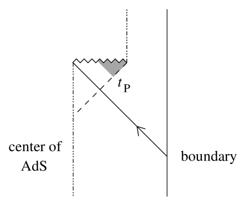
Figure 6: In an evaporating black hole trans-horizon entanglement is lost at the Page time $t_{\rm P}$, so local outgoing degrees of freedom do not exist in the shaded region.

Thus the CFT leads us to an asymmetric picture of the interior of an old black hole, illustrated in Fig. 6. According to the outgoing modes, which are responsible for Hawking evaporation, a local geometry exists in the interior only as long as the interior has a specific pattern of entanglement with the outside. But according to the ingoing modes, which are capable of describing infalling classical observers, a well-defined classical interior geometry exists at all times.

In this sense AdS/CFT reconciles unitarity of the evaporation process with the classical geometry seen by an infalling observer.

9 Conclusions

In this paper we used the construction of local bulk observables to gain insight into the black hole interior. We found that in a one-sided geometry the CFT makes a sharp distinction between ingoing and outgoing fields. Ingoing fields can be represented as conventional smeared operators in the CFT and can be used to describe infalling geodesics. Outside the horizon the outgoing fields can be represented as conventional CFT operators. In the interior they can only be accessed using entanglement. But past the Page time the trans-horizon entanglement no longer agrees with supergravity expectations, which means there is no CFT representation of local right-moving degrees of freedom in the interior. It seems the existence of a local internal geometry depends on entanglement, as suggested in [51].

It’s tempting to speculate that this partial breakdown of locality provides a mechanism for transporting information out of the black hole interior. Up to the Page time outgoing modes in the interior can be described via their pairwise entanglement with supergravity degrees of freedom outside the black hole. Note that these outgoing modes have propagated through the infalling matter, so their quantum state should be sensitive to the details of the matter that fell in to make the black hole. Starting around the Page time these outgoing degrees of freedom no longer have a local description. There are still outgoing degrees of freedom inside the black hole – the black hole still has entropy, and entanglement across the horizon is given by the Page curve – but these degrees of freedom no longer behave locally. This opens the possibility for them to transport information about the state of the infalling matter out to a stretched horizon where locality is restored.

There are many directions in which this new picture of the black hole interior could be further developed and understood. In this paper we only considered free scalar fields. It would be interesting to extend the results to fields with spin and understand the subtleties associated with gauge invariance [52, 53]. Perhaps more importantly, it would be interesting to extend the construction beyond the free-field limit. In this paper we have shown that the CFT provides a description of infalling geodesics even after the Page time. This is consistent with, but does not imply, the idea that an infalling observer experiences a smooth horizon. For example the observer could carry a particle detector (or a thermometer) coupled to the field, or could be performing experiments at low energy in the observer’s frame. To what extent can such observations and experiments be described by the CFT, and do they give results that are consistent with a smooth horizon?

Acknowledgements

We are grateful to Dorit Aharonov, Max Brodheim, Gary Gibbons and Ian Morrison for valuable discussions. We thank the Aspen Center for Physics and the KITP for hospitality. At ACP this work was supported in part by National Science Foundation grant PHY-1066293 and at KITP by NSF grant PHY11-25915. DK is supported by U.S. National Science Foundation grants PHY-1214410 and PHY-1519705 and is grateful to the Columbia University Center for Theoretical Physics for hospitality. GL is supported in part by the Israel Science Foundation under grant 504/13 and thanks the City University of New York for hospitality.

Appendix A Geodesics in AdS₂

To obtain the massive geodesics used in section 7 it’s convenient to represent AdS₂ as a hyperboloid

$$-(X^{0})^{2}-(X^{1})^{2}+(X^{2})^{2}=-R^{2}$$ (94)

inside ${\mathbb{R}}^{2,1}$ with metric

$$ds^{2}=-(dX^{0})^{2}-(dX^{1})^{2}+(dX^{2})^{2}$$ (95)

The obvious timelike geodesic winds around the waist of the hyperboloid.

$$X^{0}=R\cos(\tau/R)$$

$$X^{1}=R\sin(\tau/R)$$ (96)

$$X^{2}=0$$

A more general geodesic can be obtained by acting with a Lorentz boost.

$$\left(\begin{array}[]{c}X^{0}\\ X^{1}\\ X^{2}\end{array}\right)=\left(\begin{array}[]{ccc}\cosh\phi&0&\sinh\phi\\ 0&1&0\\ \sinh\phi&0&\cosh\phi\end{array}\right)\left(\begin{array}[]{c}R\cos(\tau/R)\\ R\sin(\tau/R)\\ 0\end{array}\right)$$ (97)

Introducing Rindler coordinates via

$$X^{0}=r\qquad X^{1}=\sqrt{r^{2}-R^{2}}\,\sinh(t/R)\qquad X^{2}=\sqrt{r^{2}-R^{2}}\,\cosh(t/R)$$ (98)

the geodesic becomes

$$t(\tau)=R\tanh^{-1}\big{(}{\tan(\tau/R)/\sinh\phi}\big{)}$$ (99)

$$r(\tau)=R\cos(\tau/R)\cosh\phi$$

In terms of the Kruskal coordinates introduced in (21), and setting $\cosh\phi=1/\cos\chi$, this gives (73).

In fact $\chi$ parametrizes the energy of the geodesic. To see this note that for a particle of mass $m$ a metric of the form (5) gives rise to a conserved energy $E=mf(r){dt\over d\tau}$. Evaluating this on (99) gives $E=m\sinh\phi=m\tan\chi$.

Appendix B Small unstable black holes in AdS

In section 8.3 we considered black holes in AdS which are formed from collapse and subsequently evaporate. Such black holes can be described in terms of the CFT, but one has to work in a non-’t Hooft limit. Here we review the construction, following the work of Horowitz [46].

For definiteness we consider four-dimensional ${\cal N}=4$ supersymmetric $SU(N)$ Yang-Mills with ’t Hooft coupling $\lambda=g^{2}_{\rm YM}N$, dual to string theory on AdS${}_{5}\times S^{5}$ with string coupling and AdS radius

$$g_{s}=g^{2}_{\rm YM}=\lambda/N\qquad\quad R=\lambda^{1/4}\ell_{s}$$ (100)

The 10-dimensional Planck length is

$$\ell_{P}=g_{s}^{1/4}\ell_{s}=R/N^{1/4}$$ (101)

The thermal phases of interest are

• a 10-dimensional supergravity gas with microcanonical entropy

  $$S_{\rm gas}\sim(RE)^{9/10}$$ (102)

• a stringy Hagedorn phase with entropy

  $$S_{\rm Hagedorn}\sim E\ell_{s}$$ (103)

• a 10-dimensional black hole which is small in the sense that the Schwarzschild radius $R_{S}<R$. The energy and entropy are

  $$E_{\rm bh}\sim R_{S}^{7}/\ell_{P}^{8}\qquad\quad S_{\rm bh}\sim R_{S}^{8}/\ell_{P}^{8}$$ (104)

We’re interested in black holes that behave much as in flat space, that are formed from collapse and subsequently evaporate to a gas of gravitons. To achieve this in AdS/CFT we want

• $\lambda>1$ and $N>1$ so the AdS radius is large compared to the string and Planck lengths: $R>\ell_{s}$ and $R>\ell_{P}$

• $N>\lambda$ so the string theory is weakly-coupled: $g_{s}<1$ and $\ell_{P}<\ell_{s}$

• a Schwarzschild radius which is large compared to the string and Planck lengths, so the black hole behaves semiclassically

• a Schwarzschild radius which satisfies $R_{S}<R/N^{2/17}$, so the black hole has less entropy than a graviton gas of the same energy: $S_{\rm bh}<S_{\rm gas}$. Such a black hole is unstable and will evaporate.

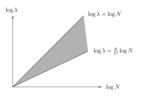
Figure 7: The range of Yang-Mills parameters for which small unstable black holes exist in AdS₅.

To summarize we’re interested in the range of parameters shown in Fig. 7,

$$N\gg\lambda\gg 1\quad{\rm and}\quad\lambda^{1/4}\gg N^{2/17}$$ (105)

Given such parameters there’s a range of Schwarzschild radii for which

$$\ell_{P}\ll\ell_{s}\ll R_{S}\ll R/N^{2/17}\ll R$$ (106)

In this range we have

$$S_{\rm Hagedorn}\ll S_{\rm bh}\ll S_{\rm gas}$$ (107)

and the black hole evaporates as though it were in flat space. Note that such black holes do not exist in the usual strongly-coupled ’t Hooft limit, where $N\rightarrow\infty$ with $\lambda\gg 1$ fixed.

Appendix C Fields inside an eternal black hole

In section 8.1 we gave a prescription for defining the field in the future interior of an eternal black hole as a sum $\phi_{\rm in}^{L}+\phi_{\rm in}^{R}$ of ingoing fields from the left and right boundaries. Here we explore this prescription in more detail and show that it is compatible with other expressions in the literature.

We work in AdS₂ in the Rindler patch and consider fields with $\Delta=1$ and $\Delta=2$. Expressions for $\phi_{\rm in}^{R}$ are given in (41) and (46), but we should be more explicit about the form of $\phi_{\rm in}^{L}$. With the $i\epsilon$ prescription described in section 8.1 we find that for $\Delta=1$

$$\phi_{\rm in}^{L}=-{1\over 2R^{2}}\int\limits_{R\log(1/v)}^{\infty}\!\!dt\,{\cal O}^{L}(t)$$ (108)

and for $\Delta=2$

$$\phi_{\rm in}^{L} = -{3\over 2R^{3}}\int_{-\infty}^{R\log(1/v)}dt\,{1\over 1+uv}\,ve^{t/R}\,{\cal O}^{L}(t)$$

$$+{3\over 2R^{3}}\int_{R\log(1/v)}^{\infty}dt\,{1\over 1+uv}\left(-1+uv-ue^{-t/R}\right){\cal O}^{L}(t)$$

Here ${\cal O}^{L}$ is an operator in the left CFT. Time runs up on the right boundary and down on the left, as shown in Fig. 8. A heuristic way to obtain these results is to (i) start with $\phi_{\rm in}^{R}$, (ii) replace $R\log u\rightarrow R\log(1/v)$ in the limits of integration, and (iii) change the sign of the constant term present in the smearing function at late times. Likewise to obtain $\phi_{\rm out}^{L}$ one starts with $\phi_{\rm out}^{R}$, replaces $R\log(-1/v)\rightarrow R\log(-u)$, and flips the sign of the constant term at late times.

Figure 8: The smearing function for a point in the interior is non-analytic when past-directed null rays from the bulk point hit the boundary.

For $\Delta=1$ the result for

$$\phi_{\rm interior}=\phi_{\rm in}^{L}+\phi_{\rm in}^{R}$$ (110)

agrees with (39) in [5]. But for $\Delta=2$ the two expressions are different, and it is not obvious that they will agree inside correlation functions. We will show that the expressions for $\Delta=2$ are in fact compatible by transforming to global coordinates and explaining in what sense they agree.

Kruskal and global coordinates are related by

$$u=\tan{\tau+\rho\over 2}\quad\qquad v=\tan{\tau-\rho\over 2}$$ (111)

This puts the metric in the form

$$ds^{2}={R^{2}\over\cos^{2}\rho}\big{(}-d\tau^{2}+d\rho^{2}\big{)}$$ (112)

$$-\infty<\tau<\infty\qquad-{\pi\over 2}<\rho<{\pi\over 2}$$

Global time $\tau$ is related to Rindler time on the left and right boundaries by

$$\tanh({t_{L}/R})=-\sin\tau\qquad\tanh({t_{R}/R})=+\sin\tau$$ (113)

Also the boundary fields in Rindler and global coordinates are related by

$$\phi\sim{1\over r^{\Delta}}\phi_{0}^{\rm Rindler}\sim\cos^{\Delta}\!\rho\,\phi_{0}^{\rm global}$$ (114)

which implies

$$\phi_{0}^{\rm Rindler}=(R\cos\tau)^{\Delta}\phi_{0}^{\rm global}$$ (115)

With these ingredients it is straightforward to transform $\phi_{\rm interior}$ to global coordinates. There is one more fact we need: in AdS₂, for fields with integer dimension, the antipodal map relates fields on the left and right boundaries by [5]

$$\phi_{0}^{\rm global,L}(\tau)=(-1)^{\Delta}\phi_{0}^{\rm global,R}(\tau+\pi)$$ (116)

This lets us rewrite $\phi_{\rm interior}$ in global coordinates purely in terms of the right boundary field. We find

$$\phi_{\rm interior}(\tau,\rho)={3\over 2}\int_{\tau-({\pi\over 2}-\rho)}^{\tau+({\pi\over 2}-\rho)}d\tau^{\prime}\left({1-uv\over 1+uv}\cos\tau^{\prime}-{u\over 1+uv}\big{(}1-\sin\tau^{\prime}\big{)}\right)\phi_{0}^{\rm global,R}(\tau^{\prime})$$

$$\hskip 14.22636pt-{3\over 2}\bigg{(}\int_{-\pi/2}^{\tau-({\pi\over 2}-\rho)}+\int_{\tau+({\pi\over 2}-\rho)}^{3\pi/2}\bigg{)}d\tau^{\prime}\,{v\over 1+uv}\big{(}1+\sin\tau^{\prime}\big{)}\,\phi_{0}^{\rm global,R}(\tau^{\prime})$$ (117)

(In this expression $u,v$ are the Kruskal coordinates of the bulk point.)

At this point it’s important to recognize that smearing functions are not unique. In global coordinates, for a field of integer conformal dimension, the boundary field is $2\pi$ periodic in global time but the Fourier components with frequencies $-\Delta+1,\ldots,\Delta-1$ are absent [5]. For $\Delta=2$ this means we’re free to add terms to the smearing function with time dependence $1,e^{i\tau},e^{-i\tau}$. We can use this freedom to eliminate the second line of (117), leaving

$$\phi_{\rm interior}(\tau,\rho)={3\over 2}\int_{\tau-({\pi\over 2}-\rho)}^{\tau+({\pi\over 2}-\rho)}d\tau^{\prime}\,{\cos(\tau-\tau^{\prime})-\sin\rho\over\cos\rho}\,\phi_{0}^{\rm global,R}(\tau^{\prime})$$ (118)

in agreement with the global smearing function obtained in [5]. This is another example of the non-uniqueness of smearing functions that was studied in [54, 55].

As a further check we used the expressions (46), (C) for $\phi_{\rm in}^{R}$ and $\phi_{\rm in}^{L}$ to compute a bulk-to-boundary 2-point function. Starting from thermal correlators in the CFT we recovered, as expected, a bulk-to-boundary correlator in the Kruskal vacuum.

References

- [1] D. Harlow, “Jerusalem lectures on black holes and quantum information,” arXiv:1409.1231 [hep-th].
- [2] V. Balasubramanian, P. Kraus, and A. E. Lawrence, “Bulk vs. boundary dynamics in anti-de Sitter spacetime,” Phys. Rev. D59 (1999) 046003, arXiv:hep-th/9805171.
- [3] T. Banks, M. R. Douglas, G. T. Horowitz, and E. J. Martinec, “AdS dynamics from conformal field theory,” arXiv:hep-th/9808016.
- [4] I. Bena, “On the construction of local fields in the bulk of AdS(5) and other spaces,” Phys. Rev. D62 (2000) 066007, arXiv:hep-th/9905186.
- [5] A. Hamilton, D. Kabat, G. Lifschytz, and D. A. Lowe, “Local bulk operators in AdS/CFT: A boundary view of horizons and locality,” Phys. Rev. D73 (2006) 086003, hep-th/0506118.
- [6] A. Hamilton, D. Kabat, G. Lifschytz, and D. A. Lowe, “Holographic representation of local bulk operators,” Phys. Rev. D74 (2006) 066009, hep-th/0606141.
- [7] A. Hamilton, D. Kabat, G. Lifschytz, and D. A. Lowe, “Local bulk operators in AdS/CFT: A holographic description of the black hole interior,” Phys. Rev. D75 (2007) 106001, hep-th/0612053.
- [8] I. Heemskerk, “Construction of bulk fields with gauge redundancy,” JHEP 1209 (2012) 106, arXiv:1201.3666 [hep-th].
- [9] D. Kabat, G. Lifschytz, S. Roy, and D. Sarkar, “Holographic representation of bulk fields with spin in AdS/CFT,” Phys.Rev. D86 (2012) 026004, arXiv:1204.0126 [hep-th].
- [10] D. Sarkar and X. Xiao, “Holographic representation of higher spin gauge fields,” Phys.Rev. D91 no. 8, (2015) 086004, arXiv:1411.4657 [hep-th].
- [11] V. K. Dobrev, “Intertwining operator realization of the AdS/CFT correspondence,” Nucl. Phys. B553 (1999) 559–582, arXiv:hep-th/9812194.
- [12] N. Aizawa and V. K. Dobrev, “Intertwining operator realization of anti de sitter holography,” arXiv:1406.2129 [hep-th].
- [13] D. Kabat, G. Lifschytz, and D. A. Lowe, “Constructing local bulk observables in interacting AdS/CFT,” Phys.Rev. D83 (2011) 106009, arXiv:1102.2910 [hep-th].
- [14] I. Heemskerk, D. Marolf, J. Polchinski, and J. Sully, “Bulk and transhorizon measurements in AdS/CFT,” JHEP 1210 (2012) 165, arXiv:1201.3664 [hep-th].
- [15] D. Kabat and G. Lifschytz, “CFT representation of interacting bulk gauge fields in AdS,” Phys.Rev. D87 (2013) 086004, arXiv:1212.3788 [hep-th].
- [16] D. Kabat and G. Lifschytz, “Decoding the hologram: Scalar fields interacting with gravity,” Phys.Rev. D89 no. 6, (2014) 066010, arXiv:1311.3020 [hep-th].
- [17] D. Kabat and G. Lifschytz, “Bulk equations of motion from CFT correlators,” JHEP 09 (2015) 059, arXiv:1505.03755 [hep-th].
- [18] H. Verlinde, “Poking holes in AdS/CFT: Bulk fields from boundary states,” arXiv:1505.05069 [hep-th].
- [19] M. Miyaji, T. Numasawa, N. Shiba, T. Takayanagi, and K. Watanabe, “Continuous multiscale entanglement renormalization ansatz as holographic surface-state correspondence,” Phys. Rev. Lett. 115 no. 17, (2015) 171602, arXiv:1506.01353 [hep-th].
- [20] Y. Nakayama and H. Ooguri, “Bulk locality and boundary creating operators,” JHEP 10 (2015) 114, arXiv:1507.04130 [hep-th].
- [21] D. Marolf and J. Polchinski, “Gauge/gravity duality and the black hole interior,” Phys.Rev.Lett. 111 (2013) 171301, arXiv:1307.4706 [hep-th].
- [22] K. Papadodimas and S. Raju, “An infalling observer in AdS/CFT,” JHEP 1310 (2013) 212, arXiv:1211.6767 [hep-th].
- [23] K. Papadodimas and S. Raju, “State-dependent bulk-boundary maps and black hole complementarity,” Phys.Rev. D89 no. 8, (2014) 086010, arXiv:1310.6335 [hep-th].
- [24] K. Papadodimas and S. Raju, “Comments on the necessity and implications of state-dependence in the black hole interior,” arXiv:1503.08825 [hep-th].
- [25] A. Almheiri, D. Marolf, J. Polchinski, and J. Sully, “Black holes: Complementarity or firewalls?,” JHEP 1302 (2013) 062, arXiv:1207.3123 [hep-th].
- [26] S. B. Giddings, “Models for unitary black hole disintegration,” Phys.Rev. D85 (2012) 044038, arXiv:1108.2015 [hep-th].
- [27] S. B. Giddings, “Nonviolent nonlocality,” Phys.Rev. D88 (2013) 064023, arXiv:1211.7070 [hep-th].
- [28] S. B. Giddings and Y. Shi, “Effective field theory models for nonviolent information transfer from black holes,” arXiv:1310.5700 [hep-th].
- [29] D. N. Page, “Expected entropy of a subsystem,” Phys. Rev. Lett. 71 (1993) 1291–1294, arXiv:gr-qc/9305007.
- [30] D. N. Page, “Information in black hole radiation,” Phys. Rev. Lett. 71 (1993) 3743–3746, arXiv:hep-th/9306083 [hep-th].
- [31] S. L. Braunstein, S. Pirandola, and K. Zyczkowski, “Better late than never: Information retrieval from black holes,” Phys. Rev. Lett. 110 no. 10, (2013) 101301, arXiv:0907.1190 [quant-ph].
- [32] J. M. Deutsch, “Quantum statistical mechanics in a closed system,” Phys. Rev. A 43 (Feb, 1991) 2046–2049.
- [33] M. Srednicki, “Chaos and quantum thermalization,” Phys. Rev. E 50 (Aug., 1994) 888–901, cond-mat/9403051.
- [34] M. Srednicki, “The approach to thermal equilibrium in quantized chaotic systems,” Journal of Physics A Mathematical General 32 (Feb., 1999) 1163–1175, cond-mat/9809360.
- [35] S. H. Shenker and D. Stanford, “Black holes and the butterfly effect,” JHEP 03 (2014) 067, arXiv:1306.0622 [hep-th].
- [36] J. Polchinski, “Chaos in the black hole S-matrix,” arXiv:1505.08108 [hep-th].
- [37] J. L. F. Barbon and E. Rabinovici, “Very long time scales and black hole thermal equilibrium,” JHEP 11 (2003) 047, arXiv:hep-th/0308063 [hep-th].
- [38] D. G. Boulware, “Quantum field theory in Schwarzschild and Rindler spaces,” Phys. Rev. D 11 (Mar, 1975) 1404–1423.
- [39] T. Klosch and T. Strobl, “Classical and quantum gravity in (1+1)-dimensions. Part 2: The universal coverings,” Class. Quant. Grav. 13 (1996) 2395–2422, arXiv:gr-qc/9511081 [gr-qc].
- [40] L. Fidkowski, V. Hubeny, M. Kleban, and S. Shenker, “The black hole singularity in AdS / CFT,” JHEP 02 (2004) 014, arXiv:hep-th/0306170 [hep-th].
- [41] S. Leichenauer and V. Rosenhaus, “AdS black holes, the bulk-boundary dictionary, and smearing functions,” Phys. Rev. D88 no. 2, (2013) 026003, arXiv:1304.6821 [hep-th].
- [42] S.-J. Rey and V. Rosenhaus, “Scanning tunneling macroscopy, black holes, and AdS/CFT bulk locality,” arXiv:1403.3943 [hep-th].
- [43] I. A. Morrison, “Boundary-to-bulk maps for AdS causal wedges and the Reeh-Schlieder property in holography,” arXiv:1403.3426 [hep-th].
- [44] W. G. Unruh, “Notes on black hole evaporation,” Phys. Rev. D14 (1976) 870.
- [45] N. D. Birrell and P. C. W. Davies, Quantum fields in curved space. Cambridge Monographs on Mathematical Physics. Cambridge Univ. Press, Cambridge, UK, 1984.
- [46] G. T. Horowitz, “Comments on black holes in string theory,” Class. Quant. Grav. 17 (2000) 1107–1116, arXiv:hep-th/9910082 [hep-th].
- [47] W. Israel, “Thermo field dynamics of black holes,” Phys. Lett. A57 (1976) 107–110.
- [48] D. Harlow, “Aspects of the Papadodimas-Raju proposal for the black hole interior,” JHEP 11 (2014) 055, arXiv:1405.1995 [hep-th].
- [49] S. R. Roy and D. Sarkar, “Hologram of a pure state black hole,” Phys. Rev. D92 (2015) 126003, arXiv:1505.03895 [hep-th].
- [50] A. Almheiri, D. Marolf, J. Polchinski, D. Stanford, and J. Sully, “An apologia for firewalls,” JHEP 09 (2013) 018, arXiv:1304.6483 [hep-th].
- [51] M. Van Raamsdonk, “Building up spacetime with quantum entanglement,” Gen. Rel. Grav. 42 (2010) 2323–2329, arXiv:1005.3035 [hep-th]. [Int. J. Mod. Phys.D19,2429(2010)].
- [52] D. Harlow, “Wormholes, emergent gauge fields, and the weak gravity conjecture,” arXiv:1510.07911 [hep-th].
- [53] M. Guica and D. L. Jafferis, “On the construction of charged operators inside an eternal black hole,” arXiv:1511.05627 [hep-th].
- [54] A. Almheiri, X. Dong, and D. Harlow, “Bulk locality and quantum error correction in AdS/CFT,” JHEP 04 (2015) 163, arXiv:1411.7041 [hep-th].
- [55] E. Mintun, J. Polchinski, and V. Rosenhaus, “Bulk-boundary duality, gauge invariance, and quantum error corrections,” Phys. Rev. Lett. 115 no. 15, (2015) 151601, arXiv:1501.06577 [hep-th].