Isoscalar-isovector proton-neutron pairing and quartet condensation in $N=Z$ nuclei

Abstract

We show that the correlations generated in the ground state of $N=Z$ nuclei by the isovector and isoscalar pairing forces can be treated with high precision as a condensate of alpha-like quartets. To treat these correlations, the quartet condensation model (QCM) is extended to the treatment of spherically symmetric isovector $(T=1,J=0)$ and isoscalar $(T=0,J=1)$ pairing forces . Within QCM we discuss the competition between $T=1$ and $T=0$ pairing correlations in the case of a two-level model and for $N=Z$ nuclei with nucleons moving in the open shells above ¹⁶O, ⁴⁰Ca and ¹⁰⁰Sn. We show that in $N=Z$ systems isovector and isoscalar proton-neutron pairing correlations always coexist.

I Introduction

One of the long standing questions in nuclear structure is whether a condensate of deuteron-like proton-neutron pairs could exist in $N=Z$ nuclei, in analogy with the condensates of like-particle pairs which account rather well for the pairing correlations in heavy $N>Z$ nuclei. For systems in which the pairing force acts only among one type of nucleons, the ansatz of the pair condensate, on which all BCS-type models are based, is supported by the fact that the pair condensate is the exact ground state of the pairing Hamiltonian for nucleons moving in degenerate orbits. When the levels are not degenerate and the pairing force is state-dependent, the exact solution is not anymore a condensate of identical pairs but rather a product of distinct (complex-conjugate) pairs richardson or, equivalently, a product of distinct (real) quartets built by four identical particles sasa_su2 . However, as shown already many years ago bayman ; dietrich , the ansatz of the pair condensate (usually known as projected-BCS approach (PBCS)) provides a good approximation even for non-degenerate levels and general state-dependent interactions, under the condition that nucleons move in orbits close to the Fermi level sandulescu_bertsch .

Based on the success of BCS-type models for like-particle pairing, these models has been applied, in a generalized form, to the treatment of pairing between neutrons and protons in $N=Z$ nuclei (e.g., see the review paper goodman and the references quoted therein). However, unlike the case of like-particle pairing, the ground state of protons and neutrons moving in degenerate levels cannot be described exactly as a pair condensate. Indeed, as shown by the SU(4) model for isovector-isoscalar pairing , in the case of degenerate levels the ground state of $N=Z$ systems is exactly described by a condensate of alpha-like quartets rather than by a condensate of pairs dobes . Quartet-type correlations have been also identified numerically in the exactly solvable SU(4) model for non-degenerate levels of angular momentum $l=0$ lerma_so8 . The SU(4) pairing model is, however, not realistic enough because it neglects the role played by the spin-orbit force, which is crucial for the description of atomic nuclei. Various studies have shown that the spin-orbit force strongly hinders the proton-neutron pairing correlations in the ground and excited states of $N=Z$ nuclei pinedo ; lei_pittel ; bertsch_luo . Yet, the majority of these studies do not discuss the types of correlations induced by the proton-neutron pairing in the presence of spin-orbit interaction. In Refs. qcm_t1 ; qcm_ngz_t1 ; qcm_wigner it was shown that the ground state of realistic isovector pairing Hamiltonians can be described with high precision as a condensate of alpha-like quartets, as suggested by the exactly solvable SO(5) model dobes . However, at variance with the SO(5) model, the quartet condensation model (QCM) for realistic pairing Hamiltonians is based on collective quartets which take properly into account the spin-orbit interaction.

The isovector pairing can also be described within a quartet model in which the ground state is represented not as a product of identical quartets, as in QCM, but as a product of distinct quartets qm_t1 . This quartet model (QM), which proposes a ground state which is analogous to that of Richardson for like-particle pairing, has been recently generalized to treat the isovector-isoscalar pairing interaction qm_t1t0 and has also been employed to analyze four-body correlations in nuclei qm_prl .

The scope of the present paper is to extend the QCM formalism to the treatment of the isovector-isoscalar pairing interactions, to analyze the accuracy of this approximation with respect to the exact solution of realistic pairing Hamiltonians as well as to the QM approach and to discuss, within QCM, the effect of spin-orbit interaction on the competition between the isovector and isoscalar paring correlations. In this study we will focus on spherically symmetric pairing interactions. An extension of the QCM approach for the axially deformed isovector-isoscalar pairing interactions was recently proposed in Ref. qcm_def .

II Formalism

The isovector and isoscalar pairing correlations in nuclei are usually studied with the Hamiltonian

$$H=\sum_{i}\epsilon_{i}N_{i}+\hat{V}_{so}+g_{1}\sum_{i,k,T_{z}}\mathcal{P}^{+}_{i,T_{z}}\mathcal{P}_{k,T_{z}}+g_{0}\sum_{i,j,S_{z}}\mathcal{D}^{+}_{i,S_{z}}\mathcal{D}_{k,S_{z}}.$$ (1)

In the first term $\epsilon_{i}$ and $N_{i}$ are, respectively, the energy and the particle number operator relative to the single-particle state $i=\{n_{i},l_{i},\tau_{i}\}$, where $l_{i}$ is the orbital angular momentum and $\tau_{i}$ is the isospin projection. The Coulomb interaction between the protons is not taken into account so that the single-particle energies of protons and neutrons are assumed to be equal. The second term in Eq. (1) is the spin-orbit interaction for protons and neutrons, which has the standard expression. The third and the fourth terms are, respectively, the isovector $(T=1,S=0)$ and isoscalar $(T=0,S=1)$ pairing interactions. They are written in terms of the pair operators

$$\mathcal{P}^{+}_{i,T_{z}}=\sqrt{\frac{2l_{i}+1}{2}}[a^{+}_{i}a^{+}_{i}]^{T=1,S=0,L=0}_{T_{z}}$$ (2)

$$\mathcal{D}^{+}_{i,S_{z}}=\sqrt{\frac{2l_{i}+1}{2}}[a^{+}_{i}a^{+}_{i}]^{S=1,T=0,L=0}_{S_{z}},$$ (3)

where $L$, $S$ and $T$ are the orbital momentum, the spin and the isospin of the pairs, respectively. When the spin-orbit is neglected and the orbits are degenerate, the Hamiltonian (1) has the SO(8) symmetry. If, in addition, $g_{1}=g_{0}$, the Hamiltonian (1) has the SU(4) symmetry and can be solved analytically both for degenerate and non-degenerate levels dobes ; lerma_so8 . This is not anymore possible in the presence of the spin-orbit interaction.

The question we address in this study is whether the ground state of the Hamiltonian (1) as well as of the most general isovector-isoscalar pairing Hamiltonian (17) (see below), can be well approximated by a condensate of alpha-like quartets, as in the case of isovector pairing qcm_t1 . Thus, as in Ref.qcm_t1 , we represent the ground state as a product of identical quartets

$$|\Psi_{gs}\rangle=(Q^{+})^{n_{q}}|0\rangle.$$ (4)

The quartet operator $Q^{+}$ is taken as a sum of two quartets

$$Q^{+}=Q^{+}_{1}+Q^{+}_{0},$$ (5)

where $Q^{+}_{1}$ is the collective isovector quartet formed by coupling two isovector pairs to total $T=0$, i.e.,

$$Q^{+}_{1}=\sum_{j_{1}j_{2}}x_{j_{1}j_{2}}[P^{+}_{j_{1}}P^{+}_{j_{2}}]^{T=0}$$ (6)

and $Q^{+}_{0}$ is the collective isoscalar quartet built by coupling two isoscalar pairs to total $J=0$, i.e.,

$$Q^{+}_{0}=\sum_{j_{1}j_{2}j_{3}j_{4}}y_{j_{1}j_{2}j_{3}j_{4}}[D^{+}_{j_{1}j_{2}}D^{+}_{j_{3}j_{4}}]^{J=0}.$$ (7)

These quartet operators are expressed in terms of the pair operators in $jj$ coupling scheme:

$$P^{+}_{j,T_{z}}=\frac{1}{\sqrt{2}}[a^{+}_{j}a^{+}_{j}]^{T=1,J=0}_{T_{z}}$$ (8)

$$D^{+}_{j_{1}j_{2}J_{z}}=\frac{1}{\sqrt{1+\delta_{j_{1}j_{2}}}}[a^{+}_{j_{1}}a^{+}_{j_{2}}]^{J=1,T=0}_{J_{z}}.$$ (9)

In Ref. qcm_t1 , the QCM state was further simplified by factorizing the mixing amplitudes which define the quartets. Due to this factorization it was possible to express the quartet condensate in terms of collective pairs and to use the recurrence relations method for the evaluation of the expectation value of the Hamiltonian. If one adopts the same factorization in the present formalism, therefore assuming that $x_{j_{1}j_{2}}=\bar{x}_{j_{1}}\bar{x}_{j_{2}}$ and $y_{j_{1}j_{2}j_{3}j_{4}}=\bar{y}_{j_{1}j_{2}}\bar{y}_{j_{3}j_{4}}$, the collective quartets can be written as

$$\bar{Q}^{+}_{1}=2\Gamma^{+}_{1}\Gamma^{+}_{-1}-(\Gamma^{+}_{0})^{2}$$ (10)

$$\bar{Q}^{+}_{0}=2\Delta^{+}_{1}\Delta^{+}_{-1}-{\Delta^{+}_{0}}^{2}.$$ (11)

These quartets are expressed in terms of the collective isoscalar and isovector pairs

$$\Gamma^{+}_{T_{z}}=\sum_{j}\bar{x}_{j}P^{+}_{j,T_{z}}$$ (12)

$$\Delta^{+}_{J_{z}}=\sum_{j_{1}j_{2}}\bar{y}_{j_{1}j_{2}}D^{+}_{j_{1}j_{2}J_{z}}.$$ (13)

It is soon realized that, when formulated in terms of collective pairs, the wave function (4) becomes a complicated superposition of mixed condensates, formed by all type of pairs. If the isoscalar quartet is further reduced to include only the $\Delta^{+}_{0}$ pairs, this formalism becomes formally equivalent to the one proposed in Ref.qcm_def for the treatement of the isovector-isoscalar pairing forces acting on axially deformed states.

The collective isovector and isoscalar pairs defined above can be used to construct various PBCS-type states for $N=Z$ systems. Thus, with the isovector pairs (12) can be formed the following PBCS states with well-defined numbers of protons and neutrons qcm_t1 :

$$|PBCS1\rangle=(\Gamma^{+}_{1}\Gamma^{+}_{-1})^{n_{q}}|0\rangle$$ (14)

$$|PBCS0_{iv}\rangle=(\Gamma^{+}_{0})^{2n_{q}}|0\rangle.$$ (15)

Both states have, as required, $J=0$ and $T_{z}=0$, but they do not have a well-defined total isospin. Similar PBCS states can be constructed with the isoscalar pairs (13). Of physical interest is the PBCS state

$$|PBCS0_{is}\rangle=(\Delta^{+}_{0})^{2n_{q}}|0\rangle.$$ (16)

This state has $T=0$ and $J_{z}=0$, but it has not a well-defined angular momentum. Since the states (15) and (16) are condensates, respectively, of $T=1$ and $T=0$ proton-neutron pairs, one might think that a comparison of their correlation energies could give a clear evidence on what type of proton-neutron pairing is prevailing in $N=Z$ nuclei. However, a conclusion based only on this comparison would be misleading because, as shown in the next section, the PBCS approximation is not accurate enough to describe properly the isovector and isoscalar pairing correlations.

In this work we will consider the case in which the mixing amplitudes $x_{ii^{\prime}}$ and $y_{ii^{\prime}jj^{\prime}}$ are factorized, as discussed above, and also the case in which they keep their original form. In both cases these amplitudes will be constructed variationally by minimizing the expectation value of the pairing Hamiltonian in the QCM or PBCS-type states.

The QCM formalism proposed in this paper can also be applied to the most general spherically symmetric isovector $(T=1,J=0)$ and isoscalar $(T=0,J=1)$ pairing forces described by the Hamiltonian

$$H=\sum_{i}\epsilon_{i}N_{i}+\sum_{i,j}V^{T=1}_{J=0}(i,j)\sum_{T_{z}}P^{+}_{i,T_{z}}P_{j,T_{z}}+\sum_{i\leq j,k\leq l}V^{T=0}_{J=1}(ij,kl)\sum_{J_{z}}D^{+}_{ij,J_{z}}D_{kl,J_{z}}.$$ (17)

The pairing interactions are written in this case in terms of the non-collective pair operators (8,9), expressed in $jj$ coupling. These interactions are not limited to the pairs with total $L=0$, as in the Hamiltonian (1), and their matrix elements are state-dependent. In Ref. qm_t1t0 it was shown that the ground state of the Hamiltonian (17) can be described with high precision as a product of distinct quartets

$$|QM\rangle=\prod^{n_{q}}_{\nu=1}Q^{(\nu){\dagger}}|0\rangle\equiv\prod^{n_{q}}_{\nu=1}(Q^{(\nu){\dagger}}_{1}+Q^{(\nu){\dagger}}_{0})|0\rangle.$$ (18)

The collective isovector and isoscalar quartets introduced above have the same form as in Eqs. (6,7) but with mixing amplitudes $x^{(\nu)}_{j_{1}j_{2}}$ and $y^{(\nu)}_{j_{1}j_{2}j_{3}j_{4}}$ which vary with the quartets. Since in (18) the quartets are allowed to be different from each other, the quartet model (QM) state (18) is expected to be a better approximation than the QCM state (4). A comparison between the two approximations will be presented in the next section.

III Results

In the SU(4) limit and for degenerate single-particle orbits the QCM state (4) provides the exact solution of the Hamiltonian (1). In the following we shall examine how accurate the QCM ansatz remains beyond the SU(4) limit and how the spin-orbit interaction affects the competition between the isovector and isoscalar pairing correlations. In order to address these issues we first apply the QCM formalism to the simple case of one orbit with angular momentum $l$. More precisely, we consider the orbit with $l=3$ and we do calculations for systems with 2, 4 and 6 proton-neutron pairs. To illustrate the influence of the spin-orbit interaction on pairing correlations, we perform calculations separately for the isovector and isoscalar pairing Hamiltonians (assuming $g_{1}$=-1, $g_{0}$=0 and $g_{1}$=0, $g_{0}$=-1, respectively, in Eq. (1)) and we change progressively the energy splitting between the states $f_{7/2}$ and $f_{5/2}$ from 0 to $7$ MeV, which is about the spin-orbit energy splitting used in realistic calculations in the $pf$ shell.

In Fig. 1 we show how the pairing correlations energy, defined as the difference between the ground state energies calculated without and with the pairing force, evolves with the spin-orbit energy splitting for the two pairing Hamiltonians. When the spin-orbit interaction is zero, the two pairing correlations energies are equal to each other; they are also equal to the exact values since in the absence of spin-orbit interaction the exact solution for the isovector (isoscalar) Hamiltonian is a QCM state formed by isovector (isoscalar) quartets. When the spin orbit is switched on, the pairing correlations energies decrease. One can notice, however, that this decrease is much stronger for the isoscalar pairing and also that it becomes more pronounced with increasing the number of proton-neutron pairs.

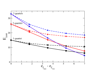
Figure 1: Correlation energies (in MeV) provided by the QCM approach in corresponence with the Hamiltonian (1) for 1, 2 and 3 quartets moving in the orbits $f_{7/2}$ and $f_{5/2}$. Dashed lines refer to the isovector Hamiltonian ($g_{1}$=-1, $g_{0}$=0) while full lines refer to the isoscalar Hamiltonian ($g_{1}$=0, $g_{0}$=-1). On the horizontal axis we show the spin-orbit energy splitting between the two orbits (in MeV).

The suppression of the pairing correlations caused by the spin-orbit interaction can in fact be expected from the matrix elements of the $S=0$ and $S=1$ pairing forces calculated for the two-body wave functions expressed in $jj$ coupling. Indeed, the diagonal matrix elements in these two channels for $j=l+1/2$ are given by

$$<(jj)J=0|\sum_{T_{z}}\mathcal{P}^{+}_{T_{z}}\mathcal{P}_{T_{z}}|(jj)J=0>=\frac{2j+1}{2}$$ (19)

$$<(jj)J=0|\mathcal{\sum}_{S_{z}}\mathcal{D}^{+}_{S_{z}}\mathcal{D}_{S_{z}}|(jj)J=0>=\frac{(2j+1)(j+1)}{6j}$$ (20)

while, in the absence of spin-orbit coupling, both matrix elements are equal to $(2l+1)=2j$. Thus, when the spin-orbit is so strong that the occupancy of $j=l-1/2$ can be neglected, the matrix elements of the $S=0$ and $S=1$ pairing forces are reduced, in the limit of large $j$, by a factor 2 and 6, respectively. The ratio of the matrix elements (19) and (20) is equal to $3j/(j+1)$, which is not very far from the ratio between the values of the two pairing energies shown in Fig. 1 at maximum spin-orbit energy splitting.

To probe the accuracy of QCM results shown in Fig. 1, we have compared them with the exact results obtained by diagonalisation. In all cases the relative errors for the correlations energies, with respect to the exact values, turn out to be small (below $1\%$), except in the case of the isoscalar pairing energy at maximum spin-orbit coupling. For example, the errors for the system of 6 proton-neutron pairs corresponding to the three values of spin-orbit energy splittings $\epsilon_{f_{5/2}}-\epsilon_{f_{7/2}}=\{3.50,5.25,7\}$ are equal, respectively, to $0.07\%$, $0.08\%$ and $0.5\%$ for isovector pairing and to $0.04\%$, $0.7\%$ and $16.7\%$ for isoscalar pairing. The large error for the isoscalar pairing at maximum spin-orbit energy splitting is related to the fact that in this case the exact ground state of the isoscalar Hamiltonian is a state with $J=2$ rather than $J=0$. Therefore the QCM result is compared not with the exact ground state of the isoscalar pairing Hamiltonian but with the first excited state with $J=0$. A similar situation occurs in the limit of very large spin-orbit splitting when all the nucleons occupy the $f_{7/2}$ orbit. On the other hand, in this limit the QCM state provides an exact solution for the ground state of the isovector pairing Hamiltonian.

Next we discuss the competition between the isovector and isoscalar pairing correlations for different values of the two pairing strengths. We assume a spin-orbit energy splitting equal to 7 MeV and parametrize the pairing strengths as $g_{0}=-(1+x)/2$ and $g_{1}=-(1-x)/2$, with $x$ ranging from -1 to 1. We recall that in many studies the physical value for the ratio between the two pairing strengths is assumed to be about 1.5 (e.g, see Ref. gerzelis_bertsch ), which corresponds to $x=0.2$. With the parameters given above we calculated the ground state energies provided by the QCM state (4) and by exact diagonalization. The comparison with the exact results shows that the accuracy of QCM is decreasing with the increasing of the mixing parameter $x$. For example, the errors for the correlation energies corresponding to $x=\{-0.5,0,0.5\}$ are, respectively, 0.04$\%$, 0.1$\%$, and 2.1$\%$. This shows that QCM provides accurate results for the physical region of the mixing parameter ($x\approx 0.2$).

The QCM results for pairing energies, defined by the average of the pairing forces in the QCM state, are shown in Fig. 2a. It can be observed that going from a pure isovector force to a pure isoscalar force the pairing energies evolve smoothly. The same behavior can be observed in Fig. 2b for the overlaps $<QCM|QCM(T=1)>$ and $<QCM|QCM(T=0)>$, where the states $QCM(T=1)$ and $QCM(T=0)$ are the components of the $QCM$ state formed only with the isovector quartet (6) and, respectively, the isoscalar quartet (7). The most important message of Fig. 2 is that the isovector and isoscalar pairing correlations coexist for any ratio of the two pairing forces. A similar conclusion was obtained recently for the isovector and isoscalar pairing forces acting on time-reversed axially deformed states qcm_def . It is worth stressing that the majority of HFB calculations for isovector-isoscalar pairing predict the coexistence of the two pairing phases only for particular pairing forces and/or nuclei goodman_prc ; gerzelis_bertsch .

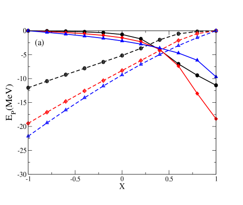
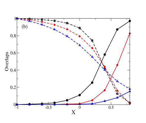
Figure 2: Pairing energies (left panel) and the overlaps $<QCM|QCM(T=1)>$ and $<QCM|QCM(T=0)>$ (right panel) as a function of the parameter $x$ which scales the strengths of the interactions (see text). The results refer to systems of 1, 2 and 3 quartets moving in the orbits $f_{7/2}$ and $f_{5/2}$ and they are shown with the same symbols adopted in Fig. 1. The energy splitting between the orbits is equal to 7 MeV.

In what follows we present applications of the QCM approach to more realistic systems. As in previous quartet model studies, we consider the $N=Z$ systems composed by nucleons moving in the valence shells above the cores ¹⁶O, ⁴⁰Ca and ¹⁰⁰Sn. First, we present the results obtained with the pairing Hamiltonian (1). As strengths of the pairing interactions we adopt the values $g_{1}=-0.377$ and $g_{0}=-0.587$ (in MeV). These pairing strengths have been suggested in Ref.zuker for the $pf$-shell nuclei. For the sake of simplicity, here we use the same pairing strengths for all nuclei. In this way, keeping the ratio of the pairing strength unchanged, we can probe how the competition between the isovector and isoscalar pairing correlations depends on the orbits and the spin-orbit splitting. The dependence of the pairing strengths on the atomic mass is taken into account through the factors $(18/A)^{0.3}$ for $sd$-shell nuclei, $(42/A)^{0.3}$ for $pf$-shell nuclei article_beta and $(102/A)^{0.3}$ for nuclei above ¹⁰⁰Sn. For the three sets of nuclei the single-particle energies, which include the spin-orbit splitting, have been taken as in shell model (SM) calculations performed with the interactions USDB usd , KB3G kb3g and with the G-matrix interaction of Ref. gmatrix . The results are presented in Table I. In the second column we show the pairing correlations energies and, in brackets, the errors relative to the exact results got by diagonalisation. It can be seen that these errors are very small. In Table I we also show the pairing energies obtained by averaging the isovector and the isoscalar pairing forces in the QCM state. We notice that for all nuclei the pairing energies are significant in both channels.

Table 1: Results of QCM calculations for $N=Z$ nuclei in various shells obtained with the Hamiltonian (1) . $E_{corr}$ are the correlations energies while $E_{P}^{T}$ are the isovector ($T=1$) and isoscalar ($T=0$) pairing energies obtained by averaging the pairing forces on the QCM state. In brackets we show the errors relative to the exact results obtained by diagonalisation. All energies are in MeV.

	$E_{corr}$	$E_{P}^{(T=1)}$	$E_{P}^{(T=0)}$
20Ne	4.005 (-)	-2.740	-2.390
24Mg	5.914 (0.7%)	-4.545	-2.660
28Si	6.359 (0.5%)	-4.389	-3.058
44Ti	5.477 (-)	-3.486	-4.478
48Cr	8.571 (0.6%)	-6.946	-4.985
52Fe	9.812 (1.1%)	-8.576	-4.557
104Te	6.413 (-)	-5.929	-2.229
108Xe	11.195 (0.3%)	-10.860	-3.677
112Ba	14.377 (0.5%)	-14.376	-4.994

Finally we have applied the QCM approach to the most general spherically symmetric pairing Hamiltonian (17). In Table II we present the results of QCM calculations performed by employing in this Hamiltonian the same input as in Ref.qm_t1t0 . Namely, the single-particle energies and the pairing interactions for the three sets of nuclei shown in Table II are extracted from the shell model forces, respectively USDB usd , KB3G kb3g and G-matrix two-body force of Ref. gmatrix . In Table II the QCM results are compared to the exact results and to the results of the QM approximation (18) presented in Ref. qm_t1t0 . One can see that the QCM approximation, in which it is supposed that all quartets have the same structure, gives accurate results, comparable with the QM approximation. In Table II we present also the results obtained with the quartet condensate state $|\overline{QCM}\rangle=(\bar{Q}^{+}_{1}+\bar{Q}^{+}_{0})^{n_{q}}|0>$ constructed with the quartets introduced in Eqs.(10,11), expressed in terms of collective pairs. One can notice that $\overline{QCM}$ describes less well the pairing correlations energies as compared to QCM. On the other hand, as shown in Ref. qm_t1 , the QCM and $\overline{QCM}$ approximations give very similar results when one considers only the isovector interaction. That means that the isoscalar pairing force induces genuine four-body correlations which cannot be described accurately by a product of collective pairs. In Table II we also present the results given by the QCM states constructed only by the isovector or the isoscalar quartets (10) and (11), i.e., $|\overline{QCM}_{T=1}\rangle=(\bar{Q}^{+}_{1})^{n_{q}}|0>$ and $|\overline{QCM}_{T=0}\rangle=(\bar{Q}^{+}_{0})^{n_{q}}|0>$. It can be seen that, for the present pairing interactions, the isoscalar pairing correlations are stronger than the isovector ones, with the exception of nuclei in the $sd$ shell. In all cases, however, as noticed also in the examples presented above, the isovector and isoscalar pairing correlations always coexist.

Table 2: Results of various calculations for $N=Z$ nuclei described by the Hamiltonian (17) . We show the correlations energies associated with the QCM state (4) and with the QCM approximations defined with the quartets (10-11), i.e., $|\overline{QCM}\rangle=(\bar{Q}^{+}_{1}+\bar{Q}^{+}_{0})^{n_{q}}|0>$, $|\overline{QCM}_{T=1}\rangle=(\bar{Q}^{+}_{1})^{n_{q}}|0>$ and $|\overline{QCM}_{T=0}\rangle=(\bar{Q}^{+}_{0})^{n_{q}}|0>$. By $QM$ are indicated the results of Ref. qm_t1t0 obtained with the state (18). In brackets we show the relative errors with respect to the exact results provided by diagonalisation. All energies are in MeV.

	Exact	$QM$	$QCM$	$\overline{QCM}$	$\overline{QCM}_{T=1}$	$\overline{QCM}_{T=0}$
20Ne	15.985	15.985 ( - )	15.985 ( - )	15.510 (2.97%)	14.373 (10.08%)	14.930 (6.60%)
24Mg	28.694	28.626 (0.24%)	28.595 (0.34%)	27.764 (3.24%	23.229 (19.04%)	26.299 (8.35% )
28Si	35.600	35.396 (0.57%)	35.288 (0.88%)	33.913 (4.74%)	28.830 (19.02% )	32.067 (9.92%)
44Ti	7.019	7.019 ( - )	7.019 ( - )	6.302 (10.21%)	6.273 (10.63%)	4.825 (31.26%)
48Cr	11.649	11.624 (0.21%)	11.614 (0.30%)	10.674 (8.37%)	10.582 (10.67%)	7.075 (39.26%)
52Fe	13.887	13.828 (0.42%)	13.799 (0.63%)	12.971 (6.60%)	12.795 (7.92%)	9.589 (30.95%)
104Te	3.147	3.147 ( - )	3.147 ( - )	3.052 (3.02%)	3.041 (3.37%)	1.512 (51.95%)
108Xe	5.505	5.495 (0.20%)	5.489 (0.29%)	5.279 (4.10%)	5.239 (4.83%)	2.530 (54.04%)
112Ba	7.059	7.035 (0.34%)	7.017 (0.59%)	6.691 (5.21%)	6.609 (6.37%)	4.391 (37.79%)

The importance of the mixing between various pairs to preserve exactly the isospin and the angular momentum of the ground state can be seen by comparing the predictions of QCM with the PBCS approximations (14-16). As seen in Table III, the results of the PBCS approximations (14-15) and (16), which do not conserve the isospin and the angular momentum, respectively, are much less accurate than the ones provided by QCM. We also notice that for all nuclei $PBCS1$ gives more binding than $PBCS_{iv}$, while the latter gives more binding than $PBCS_{is}$, except for $sd$-shell nuclei. Thus, for $sd$-shell nuclei the condensate of isoscalar proton-neutron pairs appears to be favorite with respect to the condensate of isovector pairs while the opposite is true in the other shells. On the other hand, from Table II one also sees that the approximation $\overline{QCM}_{T=1}$, in which the isovector pairs are mixed together to form a state with good isospin, gives in $sd$-shell nuclei more binding than $PBCS_{is}$. It is therefore clear that $PBCS_{is}$ results are not by themselves enough to conclude that the ground state of $sd$-shell nuclei is mainly described by a condensate of isoscalar proton-neutron pairs. In fact, as shown in Table II and Table III, a proper description of the competition between the isovector and isoscalar pairing correlations requires a ground state in which all types of pairs are mixed together in order to conserve exactly the spin and the angular momentum.

Table 3: Correlations energies provided by the PBCS-type states (14-16) in comparison with the QCM results. In brackets we show the relative errors with respect to the exact results obtained by diagonalisation. These results have been obtained with the Hamiltonian (17) using the interactions described in the text. All energies are in MeV.

	$QCM$	$PBC1$	$PBCS0_{iv}$	$PBCS0_{is}$
20Ne	15.985 ( - )	14.011 (12.35%)	13.664 (14.52%)	13.909 (12.99%)
24Mg	28.595 (0.24%)	21.993 (23.35%)	20.516 (28.50%)	23.179 (19.22%)
28Si	35.288 (0.57%)	27.206 (23.58%)	25.293 (28.95%)	27.740 (22.19%)
44Ti	7.019 ( - )	5.712 (18.62%)	5.036 (28.25%)	4.196 (40.22%)
48Cr	11.614 (0.21%)	9.686 (16.85%)	8.624 (25.97%)	6.196 (46.81%)
52Fe	13.799 (0.42%)	11.774 (15.21%)	10.591 (23.73%)	6.673 (51.95%)
104Te	3.147 ( - )	2.814 (10.58%)	2.544 (19.16%)	1.473 (53.19%)
108Xe	5.489 (0.20%)	4.866 (11.61%)	4.432 (19.49%)	2.432 (55.82%)
112Ba	7.017 (0.34%)	6.154 (12.82%)	5.635 (20.17%)	3.026 (57.13%)

IV Summary and Conclusions

In this paper we have generalized the quartet condensation model for the treatment of spherically symmetric isovector $(T=1,J=0)$ and isoscalar $(T=0,J=1)$ pairing forces. The basic assumption of the QCM approximation is that the ground state correlations induced by these forces can be described in terms of products of identical quartets formed by coupling two neutrons and two protons to total isospin $T=0$ and total angular momentum $J=0$. The generalized QCM approach has been first applied to pairing forces formulated in terms of isovector $(T=1,S=0,L=0)$ and isoscalar $(T=0,S=1,L=0)$ pairs. For these forces we have illustrated how the spin-orbit interaction affects the pairing correlations and we have studied the competition between the isovector and isoscalar pairing. Then, the QCM approach has been applied to realistic systems described by the most general pairing Hamiltonian formulated in terms of $(T=1,J=0)$ and $(T=0,J=1)$ pairs. We have shown that for both Hamiltonians the QCM gives an accurate description of the pairing correlations. We have also shown that in the QCM approximation the correlations in the two pairing channels coexist for any admixture of isovector and isoscalar pairing forces, which confirms the findings of Refs. qm_t1t0 ; qcm_def .

We wish to conclude this paper by emphasizing the striking analogy between the like-particle and proton-neutron pairing pictures which has emerged in this study and which is also supported by our previous works on the same subject qcm_t1 ; qcm_ngz_t1 ; qcm_wigner ; qm_t1 ; qm_t1t0 ; qcm_def . Thus, if on one side a condensate of collective $J=0$ pairs provides a good approximation to the ground state of spherically symmetric like-particle pairing Hamiltonians, on the other side, as shown here, a condensate of $J=0$,$T=0$ quartets provides a good approximation to the ground state of spherically symmetric proton-neutron pairing Hamiltonians. In the case of proton-neutron pairing, then, collective quartets appear to play the same role as Cooper pairs in the case of like-particle pairing. A basic difference between the like-particle pairing and pairing in $N=Z$ systems is that in the latter one needs to couple the isospin and the spin of the pairs in order to construct wave functions with well-defined total isospin and total angular momentum. As demonstrated in this paper, in even-even $N=Z$ nuclei the quartets built by coupling two pairs to $T=0$ and $J=0$ do represent the simplest form of many-body structures whose condensate can guarantee a ground state with total $T=0$ and total $J=0$. The fact that in the quartet condensate state, which describes accurately the pairing forces in $N=Z$ nuclei, the isovector and isoscalar proton-neutron pairing correlations are strongly entangled indicates that it might be difficult to disentangle them by proton-neutron transfer reactions. If in open shell $N=Z$ nuclei the quartets are indeed strongly correlated structures acting coherently as a condensate, one would expect collective features for alpha-particle transfer reactions (e.g., significant enhancement of the transfer with the number of quartets) rather than for the transfer of proton-neutron pairs.

Acknowledgements We thank D. Gambacurta for having provided us with the shell model results discussed in the text. This work was supported by the Romanian National Authority for Scientific Research, CNCS UEFISCDI, Project Number PN-II-ID-PCE-2011-3-0596.

References

- (1) R. W. Richardson and N. Sherman, Nucl. Phys. 52, 221 (1964); R. W. Richardson, Phys. Rev. 141,949 (1966).
- (2) M. Sambataro and N. Sandulescu, J. Phys. G: Nucl. Part. Phys. 40, 055107 (2013).
- (3) B. F. Bayman, Nucl. Phys. 15, 33 (1960).
- (4) K. Dietrich, H. J. Mang, J. H. Pradal, Phys. Rev. 135, B22 (1964).
- (5) N. Sandulescu and G. F. Bertsch, Phys. Rev. C 78, 064318.
- (6) A. L. Goodman, Adv. Nucl. Phys. 11 , 263 (1979).
- (7) J. Engel, S. Pittel, M. Stoitsov, P. Vogel, J. Dukelsky Phys Rev C 55 , 1781 (1997).
- (8) J. Dobes and S. Pittel, Phys. Rev. C 57, 688 (1998).
- (9) S. Lerma H., B. Errea, J. Dukelsky, W. Satula Phys Rev Lett 99, 032501 (2007).
- (10) G. Martinez-Pinedo, K. Langanke, P. Vogel, Nucl. Phys. A 651, 379 (1999).
- (11) Y. Lei, S. Pittel, N. Sandulescu, A. Poves, B. Thakur, Y. M. Zhao, Phys. Rev. C 84, 044318 (2011).
- (12) G. F. Bertsch and Y. Luo, arXiv 0912.2533.
- (13) N. Sandulescu, D. Negrea, J. Dukelsky, C. W. Johnson, Phys. Rev. C 85,061303(R) (2012).
- (14) N. Sandulescu, D. Negrea, C. W. Johnson, Phys. Rev. C 86, 041302 (R) (2012).
- (15) D. Negrea and N. Sandulescu, Phys. Rev. C 90, 024322 (2014).
- (16) M. Sambataro and N. Sandulescu, Phys. Rev. C 88, 061303(R) (2013).
- (17) M. Sambataro, N. Sandulescu, and C.W. Johnson, Phys. Lett. B740, 137 (2015).
- (18) M. Sambataro and N. Sandulescu, Phys. Rev. Lett. 115, 112501 (2015).
- (19) N. Sandulescu, D. Negrea, D. Gambacurta, Phys. Lett. B 751, 348 (2015).
- (20) A. L. Goodman, Phys. Rev. C 60, 014311 (1999).
- (21) A. Gezerlis, G. F. Bertsch, Y. L. Luo, Phys. Rev. Lett. 106, 252502 (2011).
- (22) M. Dufour and A. P. Zuker, Phys. Rev. C 54, 1641 (1996).
- (23) J. Men ndez, N. Hinohara, J. Engel, G. Mart nez-Pinedo, T. R. Rodr guez, Phys. Rev. C 93 014305 (2016).
- (24) B.A. Brown and W.A. Richter, Phys. Rev. C 74, 034315 (2006).
- (25) A. Poves and G. Martinez-Pinedo, Phys. Lett B 430, 203 (1998).
- (26) M. Hjorth-Jensen et al, Phys. Rep. 261, 125 (1995).