Goodness-of-fit tests for log and exponential GARCH models

Abstract

This paper studies goodness of fit tests and specification tests for an extension of the Log-GARCH model which is both asymmetric and stable by scaling. A Lagrange-Multiplier test is derived for testing the extended Log-GARCH against more general formulations taking the form of combinations of Log-GARCH and Exponential GARCH (EGARCH). The null assumption of an EGARCH is also tested. Portmanteau goodness-of-fit tests are developed for the extended Log-GARCH. An application to real financial data is proposed.
Keywords: EGARCH, LM tests, Invertibility of time series models, log-GARCH, Portmanteau tests, Quasi-Maximum Likelihood
Mathematical Subject Classifications: 62M10; 62P20

It is now widely accepted that, to model the dynamics of daily financial returns, volatility models have to incorporate the so-called leverage effect. Among the various asymmetric GARCH processes introduced in the econometric literature, E(xponential)GARCH and Log-GARCH models share the property of specifying the dynamics of the log-volatility, rather than the volatility, as a linear combination of past variables. One advantage of such specifications is to avoid positivity constraints on the parameters, which complicate statistical inference of standard GARCH formulations. A class of (asymmetric) Log-GARCH(p,q) models was recently studied by Francq, Wintenberger and Zakoïan (2013) (FWZ). In this class, originally introduced by Geweke (1986), Pantula (1986) and Milh j (1987) (see Sucarrat, Gr nneberg and Escribano (2015) for a more recent reference), the dynamics is defined by

$$\left\{\begin{array}[]{lll}\epsilon_{t}&=&\sigma_{t}\eta_{t},\\ \log\sigma_{t}^{2}&=&\omega+\sum_{i=1}^{q}\left(\alpha_{i+}1_{\{\epsilon_{t-i}>0\}}+\alpha_{i-}1_{\{\epsilon_{t-i}<0\}}\right)\log\epsilon_{t-i}^{2}\\ &&+\sum_{j=1}^{p}\beta_{j}\log\sigma_{t-j}^{2}\end{array}\right.$$ (0.1)

where $\sigma_{t}>0$ and $(\eta_{t})$ is a sequence of independent and identically distributed (iid) variables such that $E\eta_{1}^{2}=1$.

One drawback of this model is that it is generally not stable by scaling. Indeed, if $(\epsilon_{t})$ is a solution of Model (0.1), the process $(\epsilon_{t}^{*})$ defined by $\epsilon_{t}^{*}=c\epsilon_{t}$ with $c>0$ satisfies $\epsilon_{t}^{*}=\sigma_{t}^{*}\eta_{t}$ with $\sigma_{t}^{*2}=\omega_{t-1}^{*}+\sum_{i=1}^{q}\left(\alpha_{i+}1_{\{\epsilon_{t-i}^{*}>0\}}+\alpha_{i-}1_{\{\epsilon_{t-i}^{*}<0\}}\right)\log\epsilon_{t-i}^{*2}+\sum_{j=1}^{p}\beta_{j}\log\sigma_{t-j}^{*2}$ where

$$\omega_{t-1}^{*}=\log c^{2}\left(1-\sum_{j=1}^{p}\beta_{j}-\sum_{i=1}^{q}\left(\alpha_{i+}1_{\{\epsilon_{t-i}^{*}>0\}}+\alpha_{i-}1_{\{\epsilon_{t-i}^{*}<0\}}\right)\right)$$

is not constant (except in the symmetric case where $\alpha_{i+}=\alpha_{i-}$ for all $i$). It is important that a volatility model be stable by scaling. The standard log-GARCH has the stability by scaling property, but is not able to capture the leverage effect.

In this paper, we will consider an extension of Model (0.1) which is both stable by scaling and asymmetric. Our main foci concern specification tests of this model and the comparison with the EGARCH model. The latter formulation, introduced by Nelson (1991), appears as a widely used competitor of the Log-GARCH in applications. As we will see, the two models display very similar properties and their volatility dynamics may coincide. However, the Log-GARCH and EGARCH models are not equivalent from a statistical point of view. In particular, it is obvious to invert the Log-GARCH model, i.e. to express the volatility as an explicit function of the past returns, whereas the EGARCH(1,1) is invertible only under strong restrictions on the parameters. This is a major drawback for the statistical inference of the second specification, see Wintenberger (2013) and FWZ. However, the two models are not compatible for a same series and one has to discuss if one specification is more likely to fit the data at hand than the other. It is therefore of interest to develop testing procedures for one specification against the other. This constitutes the main aim of the present paper.

The remainder of the paper is organized as follows. Section 1 introduces the extended Log-GARCH model and discusses its similarities with the EGARCH. It also provides strict stationarity conditions. Section 2 studies the asymptotic properties of the quasi-maximum likelihood (QML) estimator. Section 3 considers testing the null assumption of a Log-GARCH against more general formulations including the EGARCH. Section 4 considers the reverse problem, in which the null assumption is the EGARCH model. In Section 5, Portmanteau goodness-of-fit tests are developed for the Log-GARCH. Section 6 compares the Log-GARCH and EGARCH models for series of exchange rates.

1 Extended Log-GARCH model

Consider the Asymmetric and stable by Scaling Log-GARCH (AS-Log-GARCH) model of order ($p,q$), defined by

$$\left\{\begin{array}[]{lll}\epsilon_{t}&=&\sigma_{t}\eta_{t},\\ \log\sigma_{t}^{2}&=&\omega+\sum_{i=1}^{q}\omega_{i-}1_{\{\epsilon_{t-i}<0\}}+\sum_{j=1}^{p}\beta_{j}\log\sigma_{t-j}^{2}\\ &&+\sum_{i=1}^{q}\left(\alpha_{i+}1_{\{\epsilon_{t-i}>0\}}+\alpha_{i-}1_{\{\epsilon_{t-i}<0\}}\right)\log\epsilon_{t-i}^{2},\end{array}\right.$$ (1.1)

where $\omega$ and the components of the vectors $\boldsymbol{\omega}_{-}=(\omega_{1-},\dots,\omega_{q-})^{\prime}$, $\boldsymbol{\alpha}_{+}=(\alpha_{1+},\dots,\alpha_{q+})^{\prime}$, $\boldsymbol{\alpha}_{-}=(\alpha_{1-},\dots,\alpha_{q-})^{\prime}$, and $\boldsymbol{\beta}=(\beta_{1},\dots,\beta_{p})^{\prime}$ are real coefficients, which are not a priori subject to positivity constraints, under the same assumptions on $(\eta_{t})$ as in Model (0.1). The main features of the asymmetric Log-GARCH($p,q$) model - volatility which is not bounded below, persistence of small values, power-aggregation - continue to hold in this extended version. We refer the reader to FWZ for details. Contrary to Model (0.1), the extended formulation (1.1) is stable by scaling. Moreover, this model leads to a different interpretation of the usual leverage effect.

1.1 News Impact Curves

Compared to model (0.1), the AS-Log-GARCH model (1.1) contains additional asymmetry parameters. Through the introduction of the coefficients $\omega_{i-}$, Model (1.1) allows for an asymmetric impact of the past positive and negative returns on the log-volatility which does not depend on their magnitudes. For instance, consider the AS-Log-ARCH(1) model with $\alpha_{1+}=\alpha_{1-}=\alpha.$ We have

$$\sigma_{t}^{2}=e^{\omega+\omega_{1-}1_{\{\epsilon_{t-1}<0\}}}(\epsilon_{t-1}^{2})^{\alpha}.$$

If $\omega_{1-}>0$, a decrease of the price, whatever its amplitude, will increase the volatility by a scaling factor $e^{\omega_{1-}}.$ In the limit case where $\alpha=0$, the volatility takes only two values depending only on the sign (not the size) of the past return. Now we turn to the second leverage effect. If $\alpha_{1+}=\alpha$ and $\alpha_{1-}=\alpha+\tau$ with $\tau>0$, we have

$$\sigma_{t}^{2}=e^{\omega+\omega_{1-}1_{\{\epsilon_{t-1}<0\}}}(\epsilon_{t-1}^{2})^{\alpha}(\epsilon_{t-1}^{2})^{\tau 1_{\{\epsilon_{t-1}<0\}}}.$$ (1.2)

The effect of a large negative return ($\epsilon_{t-1}<-1$) is an increase of volatility, but the effect may be reversed for very small returns. For small but not too small returns, this effect is balanced by the presence of the scaling factor $e^{\omega_{1-}}$. To summarize, the AS-Log-GARCH is in fact capable of detecting two types of leverage: one type where the leverage effect depends on the magnitude of negative return, and one type in which it does not. The so-called News Impact Curves, displaying $\sigma_{t}$ as a function of $\epsilon_{t-1}$, are provided in Figure 1.

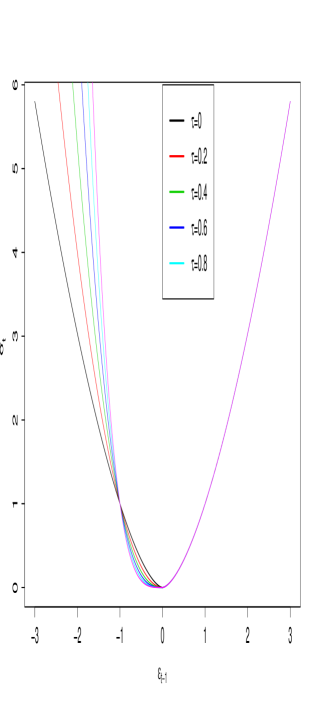
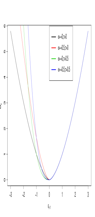
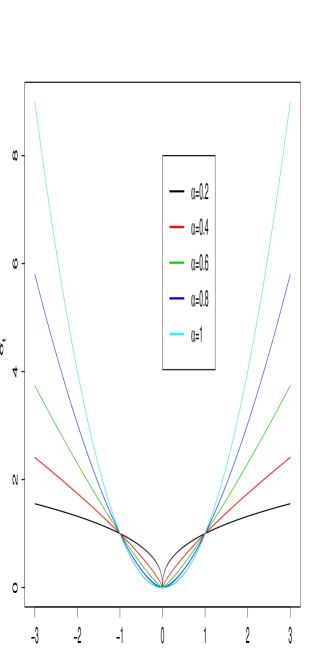
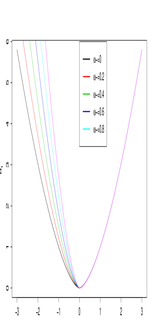
Figure 1: News Impact Curves: $\sigma_{t}$ as a function of $\epsilon_{t-1}$ in (1.2). The parameter $\omega$ is set to 0. The top graphs are obtained for $\tau=0$, the left graphs for $\omega_{-}=0$, the right graphs and the bottom left graph for $\alpha=0.8$.

1.2 Similarities with the EGARCH dynamics

The dynamics of the logarithm of the volatility of the EGARCH$(p,\ell)$ model is provided by the recursion

$$\log\sigma_{t}^{2}=\tilde{\omega}+\sum_{j=1}^{p}\tilde{\beta}_{j}\log\sigma_{t-j}^{2}+\sum_{k=1}^{\ell}\gamma_{k+}\tilde{\eta}^{+}_{t-k}+\gamma_{k-}\tilde{\eta}^{-}_{t-k},$$ (1.3)

where the innovations $\tilde{\eta}_{t}$ are iid random variables such that $E\tilde{\eta}^{2}_{1}=1$, with the notation $x^{+}=\max\{x,0\}$ and $x^{-}=\max\{-x,0\}$. If one substitutes $\log\sigma_{t-i}^{2}+\log\eta_{t-i}^{2}$ for $\log\epsilon_{t-i}^{2}$ in (1.1), the probabilistic structures of the two classes of models seem similar. More precisely, we have the following result.

Proposition 1.1

(i) For any EGARCH process $\tilde{\epsilon}_{t}=\sigma_{t}\tilde{\eta}_{t}$ satisfying (1.3) with $Ee^{s_{0}|\tilde{\eta}_{1}}|<\infty$ for some $s_{0}>0$, there exists a AS-Log-GARCH process $\epsilon_{t}=\sigma_{t}\eta_{t}$ satisfying (1.1), with the same volatility process $\sigma_{t}$ and $\eta_{t}$ measurable with respect to $\tilde{\eta}_{t}$.

(ii) Conversely, there exist AS-Log-GARCH processes $\epsilon_{t}=\sigma_{t}\eta_{t}$ for which there is no EGARCH process $\tilde{\epsilon}_{t}=\sigma_{t}\tilde{\eta}_{t}$ with the same volatility process $\sigma_{t}$ and $\tilde{\eta}_{t}$ measurable with respect to $\eta_{t}$.

Proof: Let us prove (i). For simplicity of notation, we assume that $\tilde{\epsilon}_{t}=\sigma_{t}\tilde{\eta}_{t}$ follows the first order EGARCH$(1,1)$ model, and we drop the indexes $i$, $j$ and $k$. Let the Log-GARCH(1,1) process $\epsilon_{t}=\sigma_{t}\eta_{t}$ satisfying (1.1) with the parameters $\alpha:=\alpha+=\alpha_{-}\neq 0$, $\omega+\alpha c_{+}=\tilde{\omega}$, $\omega_{-}=-\alpha(c_{-}-c_{+})$, and $\alpha+\beta=\tilde{\beta}$, and the noise $\eta_{t}=e^{\frac{c+}{2}}e^{\frac{\gamma_{+}}{2\alpha}|\tilde{\eta}_{t}|}1_{\tilde{\eta}_{t}\geq 0}-e^{\frac{c-}{2}}e^{\frac{\gamma_{-}}{2\alpha}|\tilde{\eta}_{t}|}1_{\tilde{\eta}_{t}<0},$ with constants $c_{+}$ and $c_{-}$ to be chosen later. The Log-GARCH volatility then satisfies

$$\log\sigma_{t}^{2} = \omega+\omega_{-}1_{\eta_{t-1}<0}+\alpha\log\eta_{t-1}^{2}+(\alpha+\beta)\log\sigma_{t-1}^{2}$$

$$= \tilde{\omega}+(\gamma_{+}1_{\tilde{\eta}_{t-1}>0}+\gamma_{-}1_{\tilde{\eta}_{t-1}<0})|\tilde{\eta}_{t-1}|+\tilde{\beta}\log\sigma_{t-1}^{2},$$

which is the equation satisfied by the volatility of the EGARCH(1,1) model. It then suffices to choose $\alpha$ such that $\gamma_{+}/\alpha<s_{0}$ and $\gamma_{-}/\alpha<s_{0}$, and then $c_{+}$ and $c_{-}$ such that $E\eta_{t}^{2}=1$.

Now we turn to (ii). Let $(\epsilon_{t})$ denote any AS-Log-GARCH process satisfying (1.1), with $\alpha_{1+}\neq\alpha_{1-}$, and sufficiently general so that the support of the law of $\log\sigma_{t-1}^{2}$ contains at least three different values. Also assume that $\log\eta_{t-1}^{2}$ has a finite variance. We proceed by contradiction. Suppose there exists an EGARCH process satisfying $\tilde{\epsilon}_{t}=\sigma_{t}\tilde{\eta}_{t}$ with $\tilde{\eta}_{t}=f(\eta_{t})$ for some measurable function $f$. We thus have

$$\log\sigma_{t}^{2} = \omega+\omega_{-}1_{\eta_{t-1}<0}+\left(\alpha_{1+}1_{\{\epsilon_{t-1}>0\}}+\alpha_{1-}1_{\{\epsilon_{t-1}<0\}}\right)\log\eta_{t-1}^{2}$$

$$+\left(\alpha_{1+}1_{\{\epsilon_{t-1}>0\}}+\alpha_{1-}1_{\{\epsilon_{t-1}<0\}}\right)\log\sigma_{t-1}^{2}+\sum_{j=1}^{p}\beta_{j}\log\sigma_{t-j}^{2}$$

$$= \tilde{\omega}+(\gamma_{+}1_{\tilde{\eta}_{t-1}>0}+\gamma_{-}1_{\tilde{\eta}_{t-1}<0})|\tilde{\eta}_{t-1}|+\tilde{\beta}\log\sigma_{t-1}^{2}$$

$$+\sum_{j=1}^{p}\tilde{\beta}_{j}\log\sigma_{t-j}^{2}+\sum_{k=2}^{\ell}\gamma_{k+}\tilde{\eta}^{+}_{t-k}+\gamma_{k-}\tilde{\eta}^{-}_{t-k},$$

which entails

$$a(\eta_{t-1})=b_{t-2}+c(\eta_{t-1})\log\sigma_{t-1}^{2}$$

where $b_{t-2}$ denotes a variable belonging to $\sigma$-field ${\cal F}_{t-2}$ generated by the $\eta_{t-2-j}$ with $j\geq 0$. We have

$$0 = \mbox{var}\{a(\eta_{t-1})-b_{t-2}-c(\eta_{t-1})\log\sigma_{t-1}^{2}|{\cal F}_{t-2}\}$$

$$= \mbox{var}\{a(\eta_{t-1})\}+\log^{2}\sigma_{t-1}^{2}\mbox{var}\{c(\eta_{t-1})\}-2\log\sigma_{t-1}^{2}\mbox{cov}\{a(\eta_{t-1}),c(\eta_{t-1})\},$$

from which it follows that $\log\sigma_{t-1}^{2}$ takes at most two values. This contradicts the above assumptions. $\Box$

This proposition allows to complete the interpretation of the two types of leverage effects in the AS-Log-GARCH. The coefficients $\omega_{0,i-}$ produce the leverage effect of the EGARCH volatility, i.e. an asymmetry depending on the amplitude of the innovations $\tilde{\eta}_{t-i}$. On the opposite, the EGARCH model cannot capture the asymmetric effect induced by the coefficients $\alpha_{0,i-},\alpha_{0,i+}$ and the amplitude of the returns $\epsilon_{t-i}$. Thus, the class of the Log-GARCH models generates a richer class of volatilities than the EGARCH.

1.3 Strict stationarity

We now show that the introduction of a time varying intercept in the log-volatility of Model (1.1) does not modify the strict stationarity conditions of the Log-GARCH model. The study being very similar to that of the Log-GARCH model (0.1) in FWZ, details are omitted. Let $\omega_{t}=\omega+\sum_{i=1}^{q}\omega_{i-}1_{\{\epsilon_{t-i}<0\}}$. Because coefficients equal to zero can always be added, it is not restrictive to assume $p>1$ and $q>1$. Let the vectors

$$\boldsymbol{\epsilon}_{t,q}^{+} = (1_{\{\epsilon_{t}>0\}}\log\epsilon_{t}^{2},\dots,1_{\{\epsilon_{t-q+1}>0\}}\log\epsilon_{t-q+1}^{2})^{\prime}\in\mathbb{R}^{q},$$

$$\boldsymbol{\epsilon}_{t,q}^{-} = (1_{\{\epsilon_{t}<0\}}\log\epsilon_{t}^{2},\dots,1_{\{\epsilon_{t-q+1}<0\}}\log\epsilon_{t-q+1}^{2})^{\prime}\in\mathbb{R}^{q},$$

$$\boldsymbol{z}_{t} = (\boldsymbol{\epsilon}_{t,q}^{+},\boldsymbol{\epsilon}_{t,q}^{-},\log\sigma_{t}^{2},\dots,\log\sigma_{t-p+1}^{2})^{\prime}\in\mathbb{R}^{2q+p},$$

$$\boldsymbol{b}_{t} = \left((\omega_{t}+\log\eta_{t}^{2})1_{\{\eta_{t}>0\}},\boldsymbol{0}^{\prime}_{q-1},(\omega_{t}+\log\eta_{t}^{2})1_{\{\eta_{t}<0\}},\boldsymbol{0}^{\prime}_{q-1},\omega_{t},\boldsymbol{0}^{\prime}_{p-1}\right)^{\prime}\in\mathbb{R}^{2q+p},$$

and the matrix

$$\boldsymbol{C}_{t}=\left(\begin{array}[]{ccc}1_{\{\eta_{t}>0\}}\boldsymbol{\alpha}^{\prime}_{+}&1_{\{\eta_{t}>0\}}\boldsymbol{\alpha}^{\prime}_{-}&1_{\{\eta_{t}>0\}}\boldsymbol{\beta}^{\prime}\\ \begin{array}[]{cc}\boldsymbol{I}_{q-1}&\boldsymbol{0}_{q-1}\end{array}&\boldsymbol{0}_{(q-1)\times q}&\boldsymbol{0}_{(q-1)\times p}\\ 1_{\{\eta_{t}<0\}}\boldsymbol{\alpha}^{\prime}_{+}&1_{\{\eta_{t}<0\}}\boldsymbol{\alpha}^{\prime}_{-}&1_{\{\eta_{t}<0\}}\boldsymbol{\beta}^{\prime}\\ \boldsymbol{0}_{(q-1)\times q}&\begin{array}[]{cc}\boldsymbol{I}_{q-1}&\boldsymbol{0}_{q-1}\end{array}&\boldsymbol{0}_{(q-1)\times p}\\ \boldsymbol{\alpha}^{\prime}_{+}&\boldsymbol{\alpha}^{\prime}_{-}&\boldsymbol{\beta}^{\prime}\\ \boldsymbol{0}_{(p-1)\times q}&\boldsymbol{0}_{(p-1)\times q}&\begin{array}[]{cc}\boldsymbol{I}_{p-1}&\boldsymbol{0}_{p-1}\end{array}\\ \end{array}\right).$$

Model (0.1) is rewritten in matrix form as

$$\boldsymbol{z}_{t}=\boldsymbol{C}_{t}\boldsymbol{z}_{t-1}+\boldsymbol{b}_{t}.$$

Let $\gamma({\bf C})$ be the top Lyapunov exponent of the sequence ${\bf C}=\{\boldsymbol{C}_{t},t\in\mathbb{Z}\}$,

$$\gamma({\bf C})=\lim_{t\to\infty}\frac{1}{t}E\left(\log\|\boldsymbol{C}_{t}\boldsymbol{C}_{t-1}\ldots\boldsymbol{C}_{1}\|\right)=\inf_{t\geq 1}\;\frac{1}{t}\;E(\log\|\boldsymbol{C}_{t}\boldsymbol{C}_{t-1}\ldots\boldsymbol{C}_{1}\|).$$

It can be noted that the sequence $(\boldsymbol{C}_{t},\boldsymbol{b}_{t})$ is only strictly stationary and ergodic (not iid) but this property suffices to extend the proof of Theorem 2.1 in FWZ.

Theorem 1.1

Assume that $E\log^{+}|\log\eta_{0}^{2}|<\infty$. A sufficient condition for the existence of a strictly stationary solution to the AS-Log-GARCH model (1.1) is $\gamma({\bf C})<0$. When $\gamma({\bf C})<0$, there exists only one stationary solution, which is non anticipative and ergodic.

It follows that the presence of the coefficients $\omega_{i-}$ does not modify the stationarity condition.

2 QML estimation of the AS-Log-GARCH model

We turn to the inference of the AS-Log-GARCH model. Let $\epsilon_{1},\dots,\epsilon_{n}$ be observations of the stationary solution of (1.1), where $\boldsymbol{\theta}=(\omega,\boldsymbol{\omega}_{-}^{\prime},\boldsymbol{\alpha}_{+}^{\prime},\boldsymbol{\alpha}_{-}^{\prime},\boldsymbol{\beta}^{\prime})^{\prime}$ is equal to an unknown value $\boldsymbol{\theta}_{0}$ belonging to some parameter space $\Theta\subset\mathbb{R}^{d}$, with $d=3q+p+1$. A QMLE of $\boldsymbol{\theta}_{0}$ is defined as any measurable solution $\widehat{\boldsymbol{\theta}}_{n}$ of

$$\widehat{\boldsymbol{\theta}}_{n}=\mathop{\hbox{\rm arg min}}_{\boldsymbol{\theta}\in\Theta}\widetilde{Q}_{n}(\boldsymbol{\theta}),$$ (2.1)

with

$$\widetilde{Q}_{n}(\boldsymbol{\theta})=n^{-1}\sum_{t=r_{0}+1}^{n}\widetilde{\ell}_{t}(\boldsymbol{\theta}),\qquad\widetilde{\ell}_{t}(\boldsymbol{\theta})=\frac{\epsilon_{t}^{2}}{\widetilde{\sigma}_{t}^{2}(\boldsymbol{\theta})}+\log\widetilde{\sigma}_{t}^{2}(\boldsymbol{\theta}),$$

where $r_{0}$ is a fixed integer and $\log\widetilde{\sigma}_{t}^{2}(\boldsymbol{\theta})$ is recursively defined by $\log\widetilde{\sigma}_{t}^{2}(\boldsymbol{\theta})=\omega+\sum_{i=1}^{q}\left(\alpha_{i+}\log\epsilon_{t-i}^{2}1_{\{\epsilon_{t-i}>0\}}+(\omega_{i-}+\alpha_{i-}\log\epsilon_{t-i}^{2})1_{\{\epsilon_{t-i}<0\}}\right)+\sum_{j=1}^{p}\beta_{j}\log\widetilde{\sigma}_{t-j}^{2}(\boldsymbol{\theta}),$ for $t=1,2,\dots,n$, using initial values for $\epsilon_{0},\dots,\epsilon_{1-q},\widetilde{\sigma}_{0}^{2}(\boldsymbol{\theta}),\dots,,\widetilde{\sigma}_{1-p}^{2}(\boldsymbol{\theta})$. We assume that these initial values are such that there exists a real random variable $K$ independent of $n$ satisfying

$$\sup_{\boldsymbol{\theta}\in\Theta}\left|\log\sigma_{t}^{2}(\boldsymbol{\theta})-\log\widetilde{\sigma}_{t}^{2}(\boldsymbol{\theta})\right|<K,\quad\mbox{a.s. for }t=q-p+1,\dots,q,$$ (2.2)

where $\sigma_{t}^{2}(\boldsymbol{\theta})$ is defined by

$${\cal B}_{\boldsymbol{\theta}}(B)\log\sigma_{t}^{2}(\boldsymbol{\theta}) = \omega+{\cal O}^{-}_{\boldsymbol{\theta}}(B)1_{\{\epsilon_{t}<0\}}+{\cal A}^{+}_{\boldsymbol{\theta}}(B)1_{\{\epsilon_{t}>0\}}\log\epsilon_{t}^{2}$$ (2.3)

$$+{\cal A}^{-}_{\boldsymbol{\theta}}(B)1_{\{\epsilon_{t}<0\}}\log\epsilon_{t}^{2},$$

where $B$ is the the lag operator and, for any $\boldsymbol{\theta}\in\Theta$, ${\cal A}^{+}_{\boldsymbol{\theta}}(z)=\sum_{i=1}^{q}\alpha_{i,+}z^{i}$, ${\cal A}^{-}_{\boldsymbol{\theta}}(z)=\sum_{i=1}^{q}\alpha_{i,-}z^{i}$, and ${\cal B}_{\boldsymbol{\theta}}(z)=1-\sum_{j=1}^{p}\beta_{j}z^{j}$ and ${\cal O}^{-}_{\boldsymbol{\theta}}(z)=\sum_{i=1}^{q}\omega_{i-}z^{i}$. By convention, ${\cal A}^{+}_{\boldsymbol{\theta}}(z)=0$, ${\cal A}^{-}_{\boldsymbol{\theta}}(z)=0$ and ${\cal O}^{-}_{\boldsymbol{\theta}}(z)=0$ if $q=0$, and ${\cal B}_{\boldsymbol{\theta}}(z)=1$ if $p=0$. Theorem 1.1 shows that a strict stationarity condition of the Log-GARCH can be obtained from the behaviour of the sequence ${\bf C}$. As in FWZ, it can be shown that moment conditions can be obtained by constraining the matrix

$$\boldsymbol{A}_{t} =\left(\begin{array}[]{cccc}\mu_{1}(\eta_{t-1})&\dots&\mu_{r-1}(\eta_{t-r+1})&\mu_{r}(\eta_{t-r})\\ \lx@intercol\hfil\boldsymbol{I}_{r-1}\hfil\lx@intercol&\boldsymbol{0}_{r-1}\end{array}\right),$$ (2.6)

where $r=\max(p,q)$ and $\mu_{i}(\eta_{t})=\alpha_{i+}1_{\{\eta_{t}>0\}}+\alpha_{i-}1_{\{\eta_{t}<0\}}+\beta_{i}$ with the convention $\alpha_{i+}=\alpha_{i-}=0$ for $i>p$ and $\beta_{i}=0$ for $i>q$. The spectral radius of a square matrix $\boldsymbol{A}$ is denoted by $\rho(\boldsymbol{A})$. For any vector or matrix $\boldsymbol{A}$, we denote by $\mathrm{Abs}({\boldsymbol{A}})$ the matrix whose elements are the absolute values of the corresponding elements of $\boldsymbol{A}$.

The following assumptions will be used to establish the strong consistency and asymptotic normality of the QMLE.

• $\boldsymbol{\theta}_{0}\in\Theta$ and $\Theta$ is compact.

• $\gamma\left\{{\bf C}\right\}<0\quad$ and $\quad\forall\boldsymbol{\theta}\in\Theta,\quad|{\cal B}_{\boldsymbol{\theta}}(z)|=0\Rightarrow|z|>1.$

• the support of $\eta_{0}$ contains at least two positive values and two negative values, $E\eta_{0}^{2}=1$ and $E|\log\eta_{0}^{2}|^{s_{0}}<\infty$ for some $s_{0}>0$.

• If $p>0$ and $q>1$, there is no common root to the polynomials ${\cal O}^{-}_{\boldsymbol{\theta}_{0}}(z)$, ${\cal A}^{+}_{\boldsymbol{\theta}_{0}}(z)$, ${\cal A}^{-}_{\boldsymbol{\theta}_{0}}(z)$ and ${\cal B}_{\boldsymbol{\theta}_{0}}(z)$. Moreover $(\boldsymbol{\omega}_{0-},\boldsymbol{\alpha}_{0+},\boldsymbol{\alpha}_{0-})\neq 0$ and $|\omega_{0q-}||\alpha_{0q+}||\alpha_{0q-}|+|\beta_{0p}|\neq 0$ if $p>0$.

• $E\left|\log\epsilon_{t}^{2}\right|<\infty$.

• $\boldsymbol{\theta}_{0}\in\stackrel{{\scriptstyle\circ}}{{\Theta}}$ and $\kappa_{4}:=E(\eta_{0}^{4})<\infty$.

• There exists some $s_{0}>0$ such that $E\exp(s_{0}|\log\eta_{0}^{2}|)<\infty$ and $\rho\left\{\mathrm{ess}\sup\mathrm{Abs}({\boldsymbol{A}}_{1})\right\}<1,$ where ${\boldsymbol{A}}_{1}$ is defined by (2.6).

In the case $p=q=1$, omitting the index $i$, Assumption A2 simplifies to the conditions $|\alpha_{0+}+\beta_{0}|^{a}|\alpha_{0-}+\beta_{0}|^{1-a}<1$, where $a=P(\eta_{0}>0)$, and $|\beta|<1,\forall\boldsymbol{\theta}\in\Theta$ (see FWZ, Example 2.1).

Let $\nabla Q=(\nabla_{1}Q,\dots,\nabla_{d}Q)^{\prime}$ and $\mathbb{H}Q=(\mathbb{H}_{1.}Q^{\prime},\dots,\mathbb{H}_{d.}Q^{\prime})^{\prime}$ be the vector and matrix of the first-order and second-order partial derivatives of a function $Q:\Theta\to\mathbb{R}$.

Theorem 2.1 (Asymptotic properties of the QMLE)

Let $(\widehat{\boldsymbol{\theta}}_{n})$ be a sequence of QMLE satisfying (2.1), where $(\epsilon_{t})$ is the stationary solution of the AS-Log-GARCH model (1.1) with parameter $\boldsymbol{\theta}_{0}$. Under the assumptions (2.2) and A1-A5, $\widehat{\boldsymbol{\theta}}_{n}\to\boldsymbol{\theta}_{0}$ a.s. as $n\to\infty$. If, moreover, A6-A7 hold we have $\sqrt{n}(\widehat{\boldsymbol{\theta}}_{n}-\boldsymbol{\theta}_{0})\stackrel{{\scriptstyle d}}{{\to}}\mathcal{N}(\boldsymbol{0},(\kappa_{4}-1)\bf J^{-1})$ as $n\to\infty$, where ${\bf J}=E[\nabla\log\sigma_{t}^{2}(\boldsymbol{\theta}_{0})\nabla\log\sigma_{t}^{2}(\boldsymbol{\theta}_{0})^{\prime}]$ is a positive definite matrix and $\stackrel{{\scriptstyle d}}{{\to}}$ denotes convergence in distribution.

Proof: The proof is similar to those of Theorems 4.1-4.2 of FWZ. We will only show the identifiability of the extended model, that is,

$$\sigma_{1}^{2}(\boldsymbol{\theta})=\sigma_{1}^{2}(\boldsymbol{\theta}_{0})\mbox{ a.s. }\quad\Rightarrow\quad\boldsymbol{\theta}=\boldsymbol{\theta}_{0}.$$

Note that if the left-hand side holds, by stationarity we have $\log\sigma_{t}^{2}(\boldsymbol{\theta})=\log\sigma_{t}^{2}(\boldsymbol{\theta}_{0})$ for all $t$. From the equality (2.3) we then have, almost surely,

$$\left\{\frac{{\cal O}^{-}_{\boldsymbol{\theta}}(B)}{{\cal B}_{\boldsymbol{\theta}}(B)}-\frac{{\cal O}^{-}_{\boldsymbol{\theta}_{0}}(B)}{{\cal B}_{\boldsymbol{\theta}_{0}}(B)}\right\}1_{\{\epsilon_{t}<0\}}+\left\{\frac{{\cal A}^{+}_{\boldsymbol{\theta}}(B)}{{\cal B}_{\boldsymbol{\theta}}(B)}-\frac{{\cal A}^{+}_{\boldsymbol{\theta}_{0}}(B)}{{\cal B}_{\boldsymbol{\theta}_{0}}(B)}\right\}1_{\{\epsilon_{t}>0\}}\log\epsilon_{t}^{2}$$

$$+\left\{\frac{{\cal A}^{-}_{\boldsymbol{\theta}}(B)}{{\cal B}_{\boldsymbol{\theta}}(B)}-\frac{{\cal A}^{-}_{\boldsymbol{\theta}_{0}}(B)}{{\cal B}_{\boldsymbol{\theta}_{0}}(B)}\right\}1_{\{\epsilon_{t}<0\}}\log\epsilon_{t}^{2}=\frac{\omega_{0}}{{\cal B}_{\boldsymbol{\theta}_{0}}(1)}-\frac{\omega}{{\cal B}_{\boldsymbol{\theta}}(1)}.$$

Throughout the paper let $R_{t}$ denote any generic random variable, whose value can be modified from one line to the other, which is measurable with respect to $\sigma\left(\{\eta_{u},u\leq t\}\right)$. If

$$\frac{{\cal O}^{-}_{\boldsymbol{\theta}}(B)}{{\cal B}_{\boldsymbol{\theta}}(B)}\neq\frac{{\cal O}^{-}_{\boldsymbol{\theta}_{0}}(B)}{{\cal B}_{\boldsymbol{\theta}_{0}}(B)}\;\mbox{ or }\;\frac{{\cal A}^{+}_{\boldsymbol{\theta}}(B)}{{\cal B}_{\boldsymbol{\theta}}(B)}\neq\frac{{\cal A}^{+}_{\boldsymbol{\theta}_{0}}(B)}{{\cal B}_{\boldsymbol{\theta}_{0}}(B)}\;\mbox{ or }\;\frac{{\cal A}^{-}_{\boldsymbol{\theta}}(B)}{{\cal B}_{\boldsymbol{\theta}}(B)}\neq\frac{{\cal A}^{-}_{\boldsymbol{\theta}_{0}}(B)}{{\cal B}_{\boldsymbol{\theta}_{0}}(B)},$$ (2.7)

there exists a non null $(c_{+},c_{-},d_{-})\in\mathbb{R}^{3}$, such that

$$d_{-}1_{\eta_{t}<0}+c_{+}1_{\{\eta_{t}>0\}}\log\epsilon_{t}^{2}+c_{-}1_{\{\eta_{t}<0\}}\log\epsilon_{t}^{2}+R_{t-1}=0\quad\mbox{ a.s.}$$

This is equivalent to the two equations

$$\left(c_{+}\log\eta_{t}^{2}+c_{+}\log\sigma_{t}^{2}+R_{t-1}\right)1_{\{\eta_{t}>0\}}=0\quad\mbox{ a.s.}$$

and

$$\left(d_{-}+c_{-}\log\eta_{t}^{2}+c_{-}\log\sigma_{t}^{2}+R_{t-1}\right)1_{\{\eta_{t}<0\}}=0\quad\mbox{ a.s.}$$

Note that if an equation of the form $a\log x^{2}1_{\{x>0\}}+b1_{\{x>0\}}=0$ admits two positive solutions then $a=0$. This result, A3, and the independence between $\eta_{t}$ and $(\sigma_{t}^{2},R_{t-1})$ imply that $c_{+}=0$ and $R_{t-1}=0$. Similarly we obtain $c_{-}=0$. Plugging $c_{+}=c_{-}=0$ in the equations above yields $c_{+}=c_{-}=d_{-}=0$ that is a contradiction. We conclude that (2.7) cannot hold true, and the conclusion follows from A4. $\Box$

3 Test of AS-Log-GARCH

In this section, we are interested in testing the AS-Log-GARCH specification against more general formulations, including both the Log-GARCH and the EGARCH models. For our testing problem, we therefore introduce the general model

$$\left\{\begin{array}[]{lll}\epsilon_{t}&=&\sigma_{t}\eta_{t},\\ \log\sigma_{t}^{2}&=&\omega_{0}+\sum_{i=1}^{q}\omega_{0,i-}1_{\{\epsilon_{t-i}<0\}}\\ &&+\sum_{i=1}^{q}\left(\alpha_{0,i+}1_{\{\epsilon_{t-i}>0\}}+\alpha_{0,i-}1_{\{\epsilon_{t-i}<0\}}\right)\log\epsilon_{t-i}^{2}\\ &&+\sum_{j=1}^{p}\beta_{0j}\log\sigma_{t-j}^{2}+\sum_{k=1}^{\ell}\gamma_{0,k+}\eta_{t-k}^{+}+\gamma_{0,k-}\eta_{t-k}^{-}.\end{array}\right.$$ (3.1)

Let $\boldsymbol{\vartheta}_{0}=(\boldsymbol{\theta}_{0}^{\prime},\boldsymbol{\gamma}_{0}^{\prime})^{\prime}$ where $\boldsymbol{\gamma}_{0}=(\gamma_{01,+},\gamma_{01,-},\dots,\gamma_{0\ell,-})^{\prime}$ and $\boldsymbol{\theta}_{0}$ is as in Section 2.

We wish to test the hypothesis that, in (3.1),

$$H^{\boldsymbol{\gamma}}_{0}:\boldsymbol{\gamma}_{0}=\boldsymbol{0}_{2\ell\times 1}\quad\mbox{against}\quad H_{1}^{\boldsymbol{\gamma}}:\boldsymbol{\gamma}_{0}\neq\boldsymbol{0}_{2\ell\times 1}.$$

In the time series literature, similar testing problems are solved by a standard test, using for example the Wald, Lagrange-Mutiplier (LM) or Likelihood-Ratio (LR) principle. See among others Luukkonen, Saikkonen and Ter svirta (1988), Francq, Horváth and Zako an (2010).

A difficulty, in the present framework, is that we do not have a consistent estimator of the parameter $\boldsymbol{\vartheta}_{0}$. Two problems arise to prove that the QMLE is consistent. First, the stationarity conditions of Model (3.1) are unknown. Second, due to the presence of the $|\eta_{t-k}|$’s, it seems extremely difficult to obtain invertibility conditions allowing to write $\log\sigma_{t}^{2}(\boldsymbol{\vartheta})$ (where $\boldsymbol{\vartheta}$ denotes any parameter value) as a function of the observations.

To circumvent these problems, we propose a LM approach. Denote by $\widehat{\boldsymbol{\vartheta}}_{n}^{c}$ the constrained (by $H_{0}^{\boldsymbol{\gamma}}$) estimator of $\boldsymbol{\vartheta}_{0}$, defined by

$$\widehat{\boldsymbol{\vartheta}}_{n}^{c}=(\widehat{\boldsymbol{\theta}}_{n}^{\prime},\mathbf{0}_{1\times 2\ell})^{\prime}$$

where $\widehat{\boldsymbol{\theta}}_{n}$ is the QMLE of the AS-Log-GARCH parameters defined in (2.1).

For any $\boldsymbol{\vartheta}$ in $\Theta\times\mathbb{R}^{2\ell}$, define $\log\widetilde{\sigma}_{t}^{2}(\boldsymbol{\vartheta})$ recursively, for $t=1,2,\dots,n$, by

$$\log\widetilde{\sigma}_{t}^{2}(\boldsymbol{\vartheta}) = \omega+\sum_{i=1}^{q}\omega_{i-}1_{\{\epsilon_{t-i}<0\}}+\sum_{i=1}^{q}\left(\alpha_{i+}1_{\{\epsilon_{t-i}>0\}}+\alpha_{i-}1_{\{\epsilon_{t-i}<0\}}\right)\log\epsilon_{t-i}^{2}$$

$$+\sum_{j=1}^{p}\beta_{j}\log\widetilde{\sigma}_{t-j}^{2}(\boldsymbol{\vartheta})+\sum_{k=1}^{\ell}(\gamma_{k+}\epsilon_{t-k}^{+}+\gamma_{k-}\epsilon_{t-k}^{-})e^{-\frac{1}{2}\log\widetilde{\sigma}_{t-k}^{2}(\boldsymbol{\vartheta})},$$

using positive initial values for $\epsilon_{0}^{2},\dots,\epsilon_{1-\max(q,\ell)}^{2},\widetilde{\sigma}_{0}^{2}(\boldsymbol{\vartheta}),\dots,,\widetilde{\sigma}_{1-\max(p,\ell)}^{2}(\boldsymbol{\vartheta})$. The random vector $\frac{\partial}{\partial\boldsymbol{\vartheta}}\log\widetilde{\sigma}_{t}^{2}(\boldsymbol{\vartheta})$ satisfies

$$\frac{\partial}{\partial\boldsymbol{\vartheta}}\log\widetilde{\sigma}_{t}^{2}(\boldsymbol{\vartheta}) = -\frac{1}{2}\sum_{k=1}^{\ell}(\gamma_{k+}\epsilon_{t-k}^{+}+\gamma_{k-}\epsilon_{t-k}^{-})e^{-\frac{1}{2}\log\widetilde{\sigma}_{t-k}^{2}(\boldsymbol{\vartheta})}\frac{\partial}{\partial\boldsymbol{\vartheta}}\log\widetilde{\sigma}_{t-k}^{2}(\boldsymbol{\vartheta})$$

$$+\sum_{j=1}^{p}\beta_{j}\frac{\partial}{\partial\boldsymbol{\vartheta}}\log\widetilde{\sigma}_{t-j}^{2}(\boldsymbol{\vartheta})+\left(\begin{array}[]{c}1\\ {\bf 1}_{t-1,q}^{-}\\ \boldsymbol{\epsilon}_{t-1,q}^{+}\\ \boldsymbol{\epsilon}_{t-1,q}^{-}\\ \widetilde{\boldsymbol{\sigma}}^{2}_{t-1,p}(\boldsymbol{\vartheta})\\ \widetilde{\boldsymbol{\eta}}_{t-1}(\boldsymbol{\vartheta})\end{array}\right),$$

where

$$\widetilde{\boldsymbol{\sigma}}^{2}_{t,p}(\boldsymbol{\vartheta}) = (\log\widetilde{\sigma}_{t}^{2}(\boldsymbol{\vartheta}),\ldots,\log\widetilde{\sigma}_{t-p+1}^{2}(\boldsymbol{\vartheta}))^{\prime},$$

$$\widetilde{\boldsymbol{\eta}}_{t}(\boldsymbol{\vartheta}) = (\epsilon_{t}^{+}e^{-\frac{1}{2}\log\widetilde{\sigma}_{t}^{2}(\boldsymbol{\vartheta})},\epsilon_{t}^{-}e^{-\frac{1}{2}\log\widetilde{\sigma}_{t}^{2}(\boldsymbol{\vartheta})},\ldots,\epsilon_{t-\ell+1}^{-}e^{-\frac{1}{2}\log\widetilde{\sigma}_{t-\ell+1}^{2}(\boldsymbol{\vartheta})})^{\prime}.$$

With a slight abuse of notation we write $\widetilde{\sigma}_{t}^{2}(\boldsymbol{\vartheta})=\widetilde{\sigma}_{t}^{2}(\boldsymbol{\theta})$ when $\boldsymbol{\vartheta}=(\boldsymbol{\theta}^{\prime},\mathbf{0}_{1\times 2\ell})^{\prime}$, that is when $\boldsymbol{\vartheta}$ satisfies $H_{0}^{\boldsymbol{\gamma}}$. Similarly, to avoid introducing new notations we still define the criterion function by

$$\widetilde{Q}_{n}(\boldsymbol{\vartheta})=n^{-1}\sum_{t=r_{0}+1}^{n}\widetilde{\ell}_{t}(\boldsymbol{\vartheta}),\qquad\mbox{where}\quad\widetilde{\ell}_{t}(\boldsymbol{\vartheta})=\frac{\epsilon_{t}^{2}}{\widetilde{\sigma}_{t}^{2}(\boldsymbol{\vartheta})}+\log\widetilde{\sigma}_{t}^{2}(\boldsymbol{\vartheta}).$$

To derive a LM test, we need to find the asymptotic distribution of

$$\frac{1}{\sqrt{n}}\sum_{t=1}^{n}\frac{\partial}{\partial\boldsymbol{\vartheta}}\widetilde{\ell}_{t}(\widehat{\boldsymbol{\vartheta}}_{n}^{c})=\left(\begin{array}[]{c}\mathbf{0}_{d\times 1}\\ \mathbf{S}_{n}:=\frac{1}{\sqrt{n}}\sum_{t=1}^{n}(1-\widehat{\eta}_{t}^{2})\widehat{\boldsymbol{\nu}}_{t}\end{array}\right),\quad\widehat{\boldsymbol{\nu}}_{t}={\cal B}_{\widehat{\boldsymbol{\theta}}_{n}}^{-1}(B)\widehat{\boldsymbol{\eta}}_{t-1}$$

where $\widehat{\eta}_{t}=\epsilon_{t}/\widetilde{\sigma}_{t}(\widehat{\boldsymbol{\theta}}_{n})$ for $t\geq 1$, $\widehat{\eta}_{t}=0$ for $t\leq 0$, and $\widehat{\boldsymbol{\eta}}_{t}=(\widehat{\eta}_{t}^{+},\widehat{\eta}_{t}^{-},\ldots,\widehat{\eta}_{t-\ell+1}^{-})^{\prime}.$ Note that the nullity of the first $d$ components of the score follows from the definition of $\widehat{\boldsymbol{\vartheta}}_{n}^{c}$ as a maximizer of the quasi-likelihood in the restricted model. The invertibility of the lag polynomial ${\cal B}_{\widehat{\boldsymbol{\theta}}_{n}}(B)$ follows from A2.

The following quantities are used to define the LM test statistic. Recall that $\nabla$ denotes the differentiation operator with respect to the components of $\boldsymbol{\theta}$. Let

$$\widehat{\boldsymbol{\cal J}}_{11} = \frac{1}{n}\sum_{t=1}^{n}\widehat{\boldsymbol{\nu}}_{t}\widehat{\boldsymbol{\nu}}_{t}^{\prime}-\left(\frac{1}{n}\sum_{t=1}^{n}\widehat{\boldsymbol{\nu}}_{t}\right)\left(\frac{1}{n}\sum_{t=1}^{n}\widehat{\boldsymbol{\nu}}_{t}^{\prime}\right),\quad\widehat{\kappa}_{4}-1=\frac{1}{n}\sum_{t=1}^{n}(1-\widehat{\eta}_{t}^{2})^{2},$$

$$\widehat{\bf J} = \frac{1}{n}\sum_{t=1}^{n}\nabla\log\widetilde{\sigma}_{t}^{2}(\widehat{\boldsymbol{\theta}}_{n})\nabla^{\prime}\log\widetilde{\sigma}_{t}^{2}(\widehat{\boldsymbol{\theta}}_{n}),\qquad\widehat{\boldsymbol{\Omega}}=\frac{1}{n}\sum_{t=1}^{n}\widehat{\boldsymbol{\nu}}_{t}\nabla^{\prime}\log\widetilde{\sigma}_{t}^{2}(\widehat{\boldsymbol{\theta}}_{n}),$$

$$\widehat{\boldsymbol{\cal J}}_{12} = -\left\{\widehat{\boldsymbol{\Omega}}-\left(\frac{1}{n}\sum_{t=1}^{n}\widehat{\boldsymbol{\nu}}_{t}\right)\left(\frac{1}{n}\sum_{t=1}^{n}\nabla^{\prime}\log\widetilde{\sigma}_{t}^{2}(\widehat{\boldsymbol{\theta}}_{n})\right)\right\}\widehat{\bf J}^{-1}=\widehat{\boldsymbol{\cal J}}_{21}^{\prime},$$

and

$$\widehat{\boldsymbol{\cal I}}=\widehat{\boldsymbol{\cal J}}_{11}+\widehat{\boldsymbol{\Omega}}\widehat{\bf J}^{-1}\widehat{\boldsymbol{\Omega}}^{\prime}+\widehat{\boldsymbol{\cal J}}_{12}\widehat{\boldsymbol{\Omega}}^{\prime}+\widehat{\boldsymbol{\Omega}}\widehat{\boldsymbol{\cal J}}_{21}.$$

To derive the test, we need to slightly reinforce A3 concerning the support of the distribution of $\eta_{t}$.

• The support of $\eta_{0}$ contains at least three positive values and three negative values.

Theorem 3.1 (Asymptotic distribution of the LM test under $H_{0}^{\boldsymbol{\gamma}}$)

Under the assumptions of Theorem 2.1 (thus under $H_{0}^{\boldsymbol{\gamma}}$) and A8, the matrix $\widehat{\boldsymbol{\cal I}}$ converges in probability to a positive definite matrix ${\boldsymbol{\cal I}}$ and we have

$$\mathbf{LM}_{n}^{\boldsymbol{\gamma}}=(\widehat{\kappa}_{4}-1)^{-1}\mathbf{S}_{n}^{\prime}\widehat{\boldsymbol{\cal I}}^{-1}\mathbf{S}_{n}\stackrel{{\scriptstyle d}}{{\to}}\chi^{2}_{2\ell}$$

where $\chi^{2}_{2\ell}$ denotes the chi-square distribution with $2\ell$ degrees of freedom.

Denoting by $\chi_{\ell}^{2}(\alpha)$ the $\alpha$-quantile of the chi-square distribution with $\ell$ degrees of freedom, the AS-Log-GARCH$(p,q)$ model (1.1) is then rejected at the asymptotic level $\alpha$ when $\left\{\mathbf{LM}_{n}^{\boldsymbol{\gamma}}>\chi_{2\ell}^{2}(1-\alpha)\right\}.$

Proof: For any $\boldsymbol{\vartheta}^{c}=(\boldsymbol{\theta}^{\prime},\mathbf{0}_{1\times 2\ell})^{\prime}\in\Theta\times\{0\}^{2\ell}$, let $\eta_{t}(\boldsymbol{\theta})=\frac{\epsilon_{t}}{{\sigma}_{t}(\boldsymbol{\theta})},$ $\boldsymbol{\eta}_{t}(\boldsymbol{\theta})=({\eta}_{t}^{+}(\boldsymbol{\theta}),{\eta}_{t}^{-}(\boldsymbol{\theta}),\ldots,{\eta}_{t-\ell+1}^{-}(\boldsymbol{\theta}))^{\prime},$ $\boldsymbol{\nu}_{t}(\boldsymbol{\theta})={\cal B}_{\boldsymbol{\theta}}^{-1}(B)\boldsymbol{\eta}_{t-1}(\boldsymbol{\theta})$ and let $\widetilde{\eta}_{t}(\boldsymbol{\theta}),\widetilde{\boldsymbol{\eta}}_{t}(\boldsymbol{\theta}),\widetilde{\boldsymbol{\nu}}_{t}(\boldsymbol{\theta})$ denote the corresponding quantities when ${\sigma}_{t}(\boldsymbol{\theta})$ is replaced by $\widetilde{\sigma}_{t}(\boldsymbol{\theta})$. Let also

$$\mathbf{S}_{n}(\boldsymbol{\theta})=\frac{1}{\sqrt{n}}\sum_{t=1}^{n}\{1-{\eta}_{t}^{2}(\boldsymbol{\theta})\}{\boldsymbol{\nu}}_{t}(\boldsymbol{\theta}),\quad\widetilde{\mathbf{S}}_{n}(\boldsymbol{\theta})=\frac{1}{\sqrt{n}}\sum_{t=1}^{n}\{1-\widetilde{\eta}_{t}^{2}(\boldsymbol{\theta})\}\widetilde{\boldsymbol{\nu}}_{t}(\boldsymbol{\theta}).$$

Let $\mathbf{S}_{n,i}$ denote the $i$-th component of $\mathbf{S}_{n}=\widetilde{\mathbf{S}}_{n}(\widehat{\boldsymbol{\theta}}_{n})$, for $i=1,\ldots 2\ell$. A Taylor expansion gives, for some ${\boldsymbol{\theta}}_{*}$ between $\widehat{\boldsymbol{\theta}}_{n}$ and ${\boldsymbol{\theta}}_{0}$,

$$\mathbf{S}_{n,i}=\widetilde{\mathbf{S}}_{n,i}({\boldsymbol{\theta}}_{0})+\frac{1}{\sqrt{n}}\frac{\partial\widetilde{\mathbf{S}}_{n,i}}{\partial\boldsymbol{\theta}^{\prime}}({\boldsymbol{\theta}}_{*})\sqrt{n}(\widehat{\boldsymbol{\theta}}_{n}-{\boldsymbol{\theta}}_{0}).$$ (3.4)

Recall that ${\bf J}=E[\nabla\log\sigma_{t}^{2}(\boldsymbol{\theta}_{0})\nabla\log\sigma_{t}^{2}(\boldsymbol{\theta}_{0})^{\prime}]$ and define

$$\boldsymbol{\boldsymbol{\cal J}} = \left(\begin{array}[]{cc}{\boldsymbol{\cal J}}_{11}&{\boldsymbol{\cal J}}_{12}\\ {\boldsymbol{\cal J}}_{21}&{\boldsymbol{\cal J}}_{22}\end{array}\right),\quad\mbox{where }\quad{\boldsymbol{\cal J}}_{11}=\mbox{Var}\{\boldsymbol{\nu}_{t}(\boldsymbol{\theta}_{0})\},\quad{\boldsymbol{\cal J}}_{22}={\bf J}^{-1}$$

$$\;\;\;\qquad\qquad{\boldsymbol{\cal J}}_{12}={\boldsymbol{\cal J}}_{21}^{\prime}=-\mbox{Cov}\{\boldsymbol{\nu}_{t}(\boldsymbol{\theta}_{0}),\nabla\log\sigma_{t}^{2}(\boldsymbol{\theta}_{0})\}{\bf J}^{-1},$$

and

$${\boldsymbol{\cal I}}={\boldsymbol{\cal J}}_{11}+\boldsymbol{\Omega}{\bf J}^{-1}\boldsymbol{\Omega}^{\prime}+{\boldsymbol{\cal J}}_{12}\boldsymbol{\Omega}^{\prime}+\boldsymbol{\Omega}{\boldsymbol{\cal J}}_{21},$$

where $\boldsymbol{\Omega}=E\{\boldsymbol{\nu}_{t}(\boldsymbol{\theta}_{0})\nabla^{\prime}\log\sigma_{t}^{2}(\boldsymbol{\theta}_{0})\}.$ Let $\boldsymbol{\Omega}_{i}=E\{\nu_{t,i}(\boldsymbol{\theta}_{0})\nabla^{\prime}\log\sigma_{t}^{2}(\boldsymbol{\theta}_{0})\}$, where $\nu_{t,i}(\boldsymbol{\theta}_{0})$ denotes the $i$-th component of $\boldsymbol{\nu}_{t}(\boldsymbol{\theta}_{0})$, for $i=1,\ldots 2\ell$.

The advanced result is obtained by showing the following intermediate steps: under $H_{0}^{\boldsymbol{\gamma}}$, as $n\to\infty$,

$$i)\;\sup_{\boldsymbol{\theta}\in{\cal V}(\boldsymbol{\theta}_{0})}\left\|{\mathbf{S}}_{n}(\boldsymbol{\theta})-\widetilde{\mathbf{S}}_{n}(\boldsymbol{\theta})\right\|\to 0,\quad\sup_{\boldsymbol{\theta}\in{\cal V}(\boldsymbol{\theta}_{0})}\frac{1}{\sqrt{n}}\left\|\frac{\partial{\mathbf{S}}_{n}}{\partial\boldsymbol{\theta}^{\prime}}(\boldsymbol{\theta})-\frac{\partial\widetilde{\mathbf{S}}_{n}}{\partial\boldsymbol{\theta}^{\prime}}(\boldsymbol{\theta})\right\|\to 0,$$

in probability,

$$ii)\;\left(\begin{array}[]{c}{\mathbf{S}}_{n}({\boldsymbol{\theta}}_{0})\\ \sqrt{n}(\widehat{\boldsymbol{\theta}}_{n}-{\boldsymbol{\theta}}_{0})\end{array}\right)\stackrel{{\scriptstyle d}}{{\to}}{\cal N}(\mathbf{0},(\kappa_{4}-1){\boldsymbol{\cal J}}),$$

$$iii)\;\mbox{ There exists a neighborhood of ${\cal V}(\boldsymbol{\theta}_{0})$ of $\boldsymbol{\theta}_{0}$, such that, for }i=1,\ldots,\ell$$

$$\qquad E\sup_{\boldsymbol{\theta}\in{\cal V}(\boldsymbol{\theta}_{0})}\left\|\mathbb{H}\left[\{1-\eta_{t}^{2}(\boldsymbol{\theta})\}{\cal B}_{\boldsymbol{\theta}}^{-1}(B)|\eta_{t-i}(\boldsymbol{\theta})|\right]\right\|<\infty,$$

$$iv)\;\frac{1}{\sqrt{n}}\frac{\partial{\mathbf{S}}_{n,i}}{\partial\boldsymbol{\theta}^{\prime}}(\boldsymbol{\theta}_{*})\to\boldsymbol{\Omega}_{i},\qquad\;\mbox{ in probability as $n\to\infty$,}$$

$$v)\;{\boldsymbol{\cal I}}\;\mbox{ is non-singular.}$$

We will use the following Lemma, whose proof is similar to that of Lemma 4.2 in FWZ and is thus omitted.

Lemma 3.1

Under the assumptions of Theorem 2.1, for any $m>0$ there exists a neighborhood $\mathcal{V}$ of $\boldsymbol{\theta}_{0}$ such that $E[\sup_{\mathcal{V}}(\sigma_{t}^{2}/\sigma_{t}^{2}(\boldsymbol{\theta}))^{m}]<\infty$ and $E[\sup_{\mathcal{V}}|\log\sigma_{t}^{2}(\boldsymbol{\theta})|^{m}]<\infty$.

To prove the first convergence in i), note that

$$\left\|{\mathbf{S}}_{n}(\boldsymbol{\theta})-\widetilde{\mathbf{S}}_{n}(\boldsymbol{\theta})\right\| \leq \frac{1}{\sqrt{n}}\sum_{t=1}^{n}|1-{\eta}_{t}^{2}(\boldsymbol{\theta})|\left\|{\boldsymbol{\nu}}_{t}(\boldsymbol{\theta})-\widetilde{\boldsymbol{\nu}}_{t}(\boldsymbol{\theta})\right\|$$

$$+\frac{1}{\sqrt{n}}\sum_{t=1}^{n}|\widetilde{\eta}_{t}^{2}(\boldsymbol{\theta})-{\eta}_{t}^{2}(\boldsymbol{\theta})|\left\|\widetilde{\boldsymbol{\nu}}_{t}(\boldsymbol{\theta})\right\|=S_{1}(\boldsymbol{\theta})+S_{2}(\boldsymbol{\theta}).$$

We will show that there exist $K>0$ and $\rho\in(0,1)$, such that for almost all trajectories and for all $\boldsymbol{\theta}\in\Theta,$

$$\left|\frac{1}{\sigma_{t}^{2}(\boldsymbol{\theta})}-\frac{1}{\widetilde{\sigma}_{t}^{2}(\boldsymbol{\theta})}\right|\leq\frac{K\rho^{t}}{\sigma_{t}^{2}(\boldsymbol{\theta})}.$$ (3.7)

Similarly to the proof of (7.8) in FWZ, it can be shown that

$$\sup_{\boldsymbol{\theta}\in\Theta}\frac{1}{t}\log\left|\frac{1}{\sigma_{t}^{2}(\boldsymbol{\theta})}-\frac{1}{\widetilde{\sigma}_{t}^{2}(\boldsymbol{\theta})}\right|\leq\frac{a_{1t}}{t}+a_{2t},$$

where $E|a_{1t}|<\infty$ and $\limsup_{t\to\infty}a_{2t}=\log\tilde{\rho}$ for some $\tilde{\rho}\in(0,1)$. We thus have

$$\frac{1}{t}\log\sigma_{t}^{2}(\boldsymbol{\theta})\left|\frac{1}{\sigma_{t}^{2}(\boldsymbol{\theta})}-\frac{1}{\widetilde{\sigma}_{t}^{2}(\boldsymbol{\theta})}\right|\leq\frac{\log\sigma_{t}^{2}(\boldsymbol{\theta})}{t}+\frac{a_{1t}}{t}+a_{2t}.$$

The first term in the right-hand side converges a.s. to zero as a consequence of Lemma 7.2 in FWZ and $E\sup_{\boldsymbol{\theta}\in\Theta}|\log\sigma_{t}^{2}(\boldsymbol{\theta})|<\infty$, which follows from A5. Thus (3.7) is established. Then we obtain

$$|\widetilde{\eta}_{t}^{2}(\boldsymbol{\theta})-{\eta}_{t}^{2}(\boldsymbol{\theta})|=\epsilon_{t}^{2}\left|\frac{1}{\widetilde{\sigma}_{t}^{2}(\boldsymbol{\theta})}-\frac{1}{{\sigma}_{t}^{2}(\boldsymbol{\theta})}\right|\leq\epsilon_{t}^{2}\frac{K\rho^{t}}{\sigma_{t}^{2}(\boldsymbol{\theta})}.$$

Lemma 3.1 and the $c_{r}$ and Hölder inequalities entail that for sufficiently small $s\in(0,1)$, there exists a neighborhood $\mathcal{V}$ of $\boldsymbol{\theta}_{0}$ such that

$$E\sup_{\boldsymbol{\theta}\in{\cal V}(\boldsymbol{\theta}_{0})}S_{2}^{s}(\boldsymbol{\theta}) \leq \frac{K}{n^{s/2}}\sum_{t=1}^{n}\rho^{st}E\left[|\eta_{t}|^{2s}\sup_{\boldsymbol{\theta}\in{\cal V}(\boldsymbol{\theta}_{0})}\left\{\frac{\sigma_{t}^{2s}}{\sigma_{t}^{2s}(\boldsymbol{\theta})}\left\|\widetilde{\boldsymbol{\nu}}_{t}(\boldsymbol{\theta})\right\|^{s}\right\}\right]$$

$$\leq \frac{K}{n^{s/2}}\sum_{t=1}^{n}\rho^{st}\to 0$$

as $n\to\infty$. This entails $\sup_{\boldsymbol{\theta}\in{\cal V}(\boldsymbol{\theta}_{0})}S_{2}(\boldsymbol{\theta})=o_{P}(1).$ Similarly, we have $\sup_{\boldsymbol{\theta}\in{\cal V}(\boldsymbol{\theta}_{0})}S_{1}(\boldsymbol{\theta})=o_{P}(1).$ The first convergence in i) follows and the second one is obtained by the same arguments.

To prove ii), note that

$$\left(\begin{array}[]{c}{\mathbf{S}}_{n}({\boldsymbol{\theta}}_{0})\\ \sqrt{n}(\widehat{\boldsymbol{\theta}}_{n}-{\boldsymbol{\theta}}_{0})\end{array}\right)=\frac{1}{\sqrt{n}}\sum_{t=1}^{n}(1-{\eta}_{t}^{2})\left(\begin{array}[]{c}\boldsymbol{\nu}_{t}(\boldsymbol{\theta}_{0})\\ -{\bf J}^{-1}\nabla\log\sigma_{t}^{2}(\boldsymbol{\theta}_{0})\end{array}\right)+o_{P}(1).$$

The convergence in distribution thus follows from the central limit theorem for martingale differences.

To prove iii), write ${\cal B}_{\boldsymbol{\theta}}^{-1}(B)=\sum_{j=0}^{\infty}c_{j}(\boldsymbol{\theta})B^{j}$. We have

$$\mathbb{H}\{\eta_{t}(\boldsymbol{\theta})\} = \eta_{t}(\boldsymbol{\theta})\left[\frac{1}{4}\nabla\log\sigma_{t}^{2}(\boldsymbol{\theta})\nabla^{\prime}\log\sigma_{t}^{2}(\boldsymbol{\theta})-\frac{1}{2}\mathbb{H}\{\log\sigma_{t}^{2}(\boldsymbol{\theta})\}\right],$$

$$\mathbb{H}\{1-\eta_{t}^{2}(\boldsymbol{\theta})\} = \eta_{t}^{2}(\boldsymbol{\theta})\left[-\nabla\log\sigma_{t}^{2}(\boldsymbol{\theta})\nabla^{\prime}\log\sigma_{t}^{2}(\boldsymbol{\theta})+\mathbb{H}\{\log\sigma_{t}^{2}(\boldsymbol{\theta})\}\right].$$

It follows that, dropping temporarily the term "$(\theta)$" to lighten the notation,

$$\mathbb{H}\{1-\eta_{t}^{2}\}c_{j}|\eta_{t-i-j}|$$

$$= \eta_{t}^{2}\{-\nabla\log\sigma_{t}^{2}\nabla^{\prime}\log\sigma_{t}^{2}+\mathbb{H}\log\sigma_{t}^{2}\}c_{j}|\eta_{t-i-j}|$$

$$+\{1-\eta_{t}^{2}\}\{\mathbb{H}c_{j}\}|\eta_{t-i-j}|$$

$$+\{1-\eta_{t}^{2}\}c_{j}|\eta_{t-i-j}|\{\frac{1}{4}\nabla\log\sigma_{t}^{2}\nabla^{\prime}\log\sigma_{t}^{2}-\frac{1}{2}\mathbb{H}\log\sigma_{t}^{2}\}$$

$$+\eta_{t}^{2}\{\nabla\log\sigma_{t}^{2}\nabla^{\prime}c_{j}+\nabla c_{j}\nabla^{\prime}\log\sigma_{t}^{2}\}|\eta_{t-i-j}|$$

$$-\frac{1}{2}\eta_{t}^{2}\{\nabla\log\sigma_{t}^{2}\nabla^{\prime}\log\sigma_{t-i-j}^{2}+\nabla\log\sigma_{t-i-j}^{2}\nabla^{\prime}\log\sigma_{t}^{2}\}|\eta_{t-i-j}|c_{j}$$

$$-\frac{1}{2}\{1-\eta_{t}^{2}\}\{\nabla c_{j}\nabla^{\prime}\log\sigma_{t-i-j}^{2}+\nabla\log\sigma_{t-i-j}^{2}\nabla^{\prime}c_{j}\}|\eta_{t-i-j}|.$$

In view of Lemma 3.1, since $\eta_{t}(\boldsymbol{\theta})=\eta_{t}\sigma_{t}(\boldsymbol{\theta}_{0})/\sigma_{t}(\boldsymbol{\theta})$, because $\nabla\log\sigma_{t}^{2}(\boldsymbol{\theta})$ admits moments of any order, and using the Hölder inequality, the conclusion follows.

To prove iv), consider the following Taylor expansion about $\boldsymbol{\theta}_{0}$

$$\frac{1}{\sqrt{n}}\frac{\partial{\mathbf{S}}_{n,i}}{\partial\boldsymbol{\theta}}(\boldsymbol{\theta}_{*})=\frac{1}{\sqrt{n}}\frac{\partial{\mathbf{S}}_{n,i}}{\partial\boldsymbol{\theta}}(\boldsymbol{\theta}_{0})+\frac{1}{\sqrt{n}}\frac{\partial^{2}{\mathbf{S}}_{n,i}}{\partial\boldsymbol{\theta}\partial\boldsymbol{\theta}^{\prime}}(\boldsymbol{\theta}^{*})(\boldsymbol{\theta}_{*}-\boldsymbol{\theta}_{0})$$

where $\boldsymbol{\theta}^{*}$ is between $\boldsymbol{\theta}_{*}$ and $\boldsymbol{\theta}_{0}$. The a.s. convergence of $\boldsymbol{\theta}^{*}$ to $\boldsymbol{\theta}_{0}$, iii) and the ergodic theorem imply that, for $i=2k+1$ and for some neighborhood of $\boldsymbol{\theta}_{0}$

$$\lim\sup_{n\to\infty}\left\|\frac{1}{\sqrt{n}}\frac{\partial^{2}{\mathbf{S}}_{n,i}}{\partial\boldsymbol{\theta}\partial\boldsymbol{\theta}^{\prime}}(\boldsymbol{\theta}^{*})\right\|$$

$$\leq \lim\sup_{n\to\infty}\frac{1}{n}\sum_{t=1}^{n}\sup_{\boldsymbol{\theta}\in{\cal V}(\boldsymbol{\theta}_{0})}\left\|\frac{\partial^{2}}{\partial\boldsymbol{\theta}\partial\boldsymbol{\theta}^{\prime}}\{1-\eta_{t}^{2}(\boldsymbol{\theta})\}{\cal B}_{\boldsymbol{\theta}}^{-1}(B)\eta_{t-k-1}^{+}(\boldsymbol{\theta})\right\|$$

$$= E\sup_{\boldsymbol{\theta}\in{\cal V}(\boldsymbol{\theta}_{0})}\left\|\frac{\partial^{2}}{\partial\boldsymbol{\theta}\partial\boldsymbol{\theta}^{\prime}}\{1-\eta_{t}^{2}(\boldsymbol{\theta})\}{\cal B}_{\boldsymbol{\theta}}^{-1}(B)\eta_{t-k-1}^{+}(\boldsymbol{\theta})\right\|<\infty.$$

The same argument obviously applies for $i=2k$ and the conclusion follows.

To prove v), in view of (3.4), it suffices to show that ${\boldsymbol{\cal J}}$ is non-singular. Suppose there exist ${\bf x}=(x_{i})\in\mathbb{R}^{2\ell}$ and ${\bf y}\in\mathbb{R}^{d}$ such that

$${\bf x}^{\prime}\boldsymbol{\nu}_{t}(\boldsymbol{\theta}_{0})+{\bf y}^{\prime}{\bf J}^{-1}\nabla\log\sigma_{t}^{2}(\boldsymbol{\theta}_{0})=0,\quad\mbox{a.s.}$$

Recall that, in view of (2.3),

$$\nabla\log\sigma_{t}^{2}(\boldsymbol{\theta}_{0})={\cal B}_{\boldsymbol{\theta}_{0}}^{-1}(B)\left(1,{\bf 1}^{-^{\prime}}_{t-1,q},\boldsymbol{\epsilon}_{t-1,q}^{+^{\prime}},\boldsymbol{\epsilon}_{t-1,q}^{-^{\prime}},\boldsymbol{\sigma}^{2^{\prime}}_{t-1,p}(\boldsymbol{\theta}_{0})\right)^{\prime}.$$

Letting ${\bf z}={\bf J}^{-1}{\bf y}=(z_{i})$, we find that, $x_{1}\eta_{t-1}^{+}+x_{2}\eta_{t-1}^{-}+z_{2}1_{\{\eta_{t-1}>0\}}+z_{2+q}1_{\{\eta_{t-1}>0\}}\log\epsilon_{t-1}^{2}+z_{2+2q}1_{\{\eta_{t-1}<0\}}\log\epsilon_{t-1}^{2}=R_{t-2},\quad\mbox{a.s.}$ Conditionally on $\eta_{t-1}>0$ we thus have

$$x_{1}\eta_{t-1}+z_{2}+z_{2+q}\log\eta_{t-1}^{2}+z_{2+q}\log\sigma_{t-1}^{2}=R_{t-2},\quad\mbox{a.s.}$$

By A8, we find $x_{1}=z_{2+q}=0.$ By conditioning on $\eta_{t-1}<0$, we similarly get $x_{2}=z_{2+2q}=0.$ Thus $z_{2}1_{\{\eta_{t-1}>0\}}=R_{t-2},\quad\mbox{a.s.},$ from which we deduce $z_{2}=R_{t-2}=0\quad\mbox{a.s.}$ Proceeding by induction, we show that ${\bf x}={\bf 0}$ and ${\bf z}={\bf 0}$. Finally, ${\bf y}={\bf 0}$ and the invertibility of ${\boldsymbol{\cal J}}$ is established.

It follows from Steps i)-v) and (3.4) that

$$\mathbf{S_{n}}\stackrel{{\scriptstyle d}}{{\to}}{\cal N}(\mathbf{0},(\kappa_{4}-1){\boldsymbol{\cal I}}).$$

It can also be shown that $\widehat{\boldsymbol{\cal I}}\to{\boldsymbol{\cal I}}$ and $\widehat{\kappa}_{4}\to\kappa_{4}$ in probability, from which the conclusion follows. $\Box$

4 Test of EGARCH(1,1)

In this section, we consider testing the EGARCH(1,1) specification in the framework of Model (3.1) with $p=\ell=1$. For convenience, we reparameterize it as follows

$$\left\{\begin{array}[]{lll}\epsilon_{t}&=&\sigma_{t}\eta_{t},\\ \log\sigma_{t}^{2}&=&\omega_{0}+\sum_{i=1}^{q}\omega_{0,i-}1_{\{\epsilon_{t-i}<0\}}+\gamma_{0}\eta_{t-1}+\delta_{0}|\eta_{t-1}|+\beta_{0}\log\sigma_{t-1}^{2}\\ &&+\sum_{i=1}^{q}\left(\alpha_{0,i+}1_{\{\epsilon_{t-i}>0\}}+\alpha_{0,i-}1_{\{\epsilon_{t-i}<0\}}\right)\log\epsilon_{t-i}^{2}.\end{array}\right.$$ (4.1)

Let $\boldsymbol{\vartheta}_{0}=(\boldsymbol{\zeta}_{0}^{\prime},\boldsymbol{\alpha}_{0}^{\prime})^{\prime}$ where $\boldsymbol{\zeta}_{0}=(\omega_{0},\gamma_{0},\delta_{0},\beta_{0})^{\prime}$ and $\boldsymbol{\alpha}_{0}=(\boldsymbol{\omega}_{0-}^{\prime},\boldsymbol{\alpha}_{0+}^{\prime},\boldsymbol{\alpha}_{0-}^{\prime})^{\prime}$. The vector $\boldsymbol{\zeta}_{0}$ is assumed to belong to some compact parameter set $\Xi\subset\mathbb{R}^{4}$.

We will derive a LM approach to test the hypothesis that, in (4.1),

$$H_{0}^{\boldsymbol{\alpha}}:\boldsymbol{\alpha}_{0}=0\quad\mbox{against}\quad H_{1}^{\boldsymbol{\alpha}}:\boldsymbol{\alpha}_{0}\neq 0.$$

Assuming that $|\beta_{0}|<1$, there exists a stationary solution to Model (4.1) under $H_{0}^{\boldsymbol{\alpha}}$, obtained from the MA($\infty$) representation

$$\log\sigma_{t}^{2}=\omega_{0}(1-\beta_{0})^{-1}+\sum_{k=1}^{\infty}\beta_{0}^{k-1}\{\gamma_{0}\eta_{t-k}+\delta_{0}|\eta_{t-k}|\}.$$

An important difficulty in the estimation of the EGARCH(1,1) model is that invertibility is not trivial. Invertibility is required to write $\widetilde{\sigma}_{t}^{2}(\boldsymbol{\zeta})$, to be defined below, in function of the observations $\epsilon_{t}$ for any $\boldsymbol{\zeta}=(\omega,\gamma,\delta,\beta)^{\prime}$. Wintenberger (2013) obtained the following sufficient condition for continuous invertibility of the EGARCH(1,1): the compact set $\Xi$ is included in $\mathbb{R}\times\{\delta\geq|\gamma|\}\times\mathbb{R}^{+}$ and $\forall\boldsymbol{\zeta}\in\Xi$,

$$E\left[\log\left(\max\left[\beta,\frac{1}{2}(\gamma\epsilon_{0}+\delta|\epsilon_{0}|)\exp\left\{-\frac{\omega}{2(1-\beta)}\right\}-\beta\right]\right)\right]<0.$$ (4.2)

Notice that this condition depends on the distribution of the observations $(\epsilon_{t})$.

Denote by $\widehat{\boldsymbol{\vartheta}}_{n}^{c}$ the constrained (by $H_{0}^{\boldsymbol{\alpha}}$) estimator of $\boldsymbol{\vartheta}_{0}$, defined by

$$\widehat{\boldsymbol{\vartheta}}_{n}^{c}=(\widehat{\boldsymbol{\zeta}}_{n}^{\prime},\mathbf{0}_{1\times 3q})^{\prime}$$

where $\widehat{\boldsymbol{\zeta}}_{n}$ is the QMLE of the EGARCH parameters defined by

$$\widehat{\boldsymbol{\zeta}}_{n}=\mathop{\hbox{\rm arg min}}_{\boldsymbol{\zeta}\in\Xi}\widetilde{Q}_{n}(\boldsymbol{\zeta}),$$

with

$$\widetilde{Q}_{n}(\boldsymbol{\zeta})=n^{-1}\sum_{t=r_{0}+1}^{n}\widetilde{\ell}_{t}(\boldsymbol{\zeta}),\qquad\widetilde{\ell}_{t}(\boldsymbol{\zeta})=\frac{\epsilon_{t}^{2}}{\widetilde{\sigma}_{t}^{2}(\boldsymbol{\zeta})}+\log\widetilde{\sigma}_{t}^{2}(\boldsymbol{\zeta}),$$

where $r_{0}$ is a fixed integer and $\log\widetilde{\sigma}_{t}^{2}(\boldsymbol{\zeta})$ is recursively defined by

$$\log\widetilde{\sigma}_{t}^{2}(\boldsymbol{\zeta})=\omega+\gamma\widetilde{\eta}_{t-1}(\boldsymbol{\zeta})+\delta|\widetilde{\eta}_{t-1}(\boldsymbol{\zeta})|+\beta\log\widetilde{\sigma}_{t-1}^{2}(\boldsymbol{\zeta}),\quad\widetilde{\eta}_{t-1}(\boldsymbol{\zeta})=\epsilon_{t-1}/\widetilde{\sigma}_{t-1}(\boldsymbol{\zeta})$$

using initial values for $\epsilon_{0},\widetilde{\sigma}_{0}^{2}(\boldsymbol{\zeta}).$ For any $\boldsymbol{\zeta}\in\Xi$, the continuous invertibility condition (4.2) allows to define the sequence $({\sigma}_{t}^{2}(\boldsymbol{\zeta}))_{t\in\mathbb{Z}}$ by

$$\log{\sigma}_{t}^{2}(\boldsymbol{\zeta})=\omega+\gamma{\eta}_{t-1}(\boldsymbol{\zeta})+\delta|{\eta}_{t-1}(\boldsymbol{\zeta})|+\beta\log{\sigma}_{t-1}^{2}(\boldsymbol{\zeta}),\quad{\eta}_{t-1}(\boldsymbol{\zeta})=\epsilon_{t-1}/{\sigma}_{t-1}(\boldsymbol{\zeta}).$$

We introduce the following assumption.

• $\boldsymbol{\zeta}_{0}\in\stackrel{{\scriptstyle\circ}}{{\Xi}}$, $E(\eta_{0}^{4})<\infty$ and $E\{\beta_{0}-\frac{1}{2}(\gamma_{0}\eta_{0}+\delta_{0}\left|\eta_{0}\right|)\}^{2}<1$.

The following result was established by Wintenberger (Theorem 6, 2013).

Theorem 4.1 (Asymptotics of the QMLE for the EGARCH(1,1))

For any compact subset $\Xi$ of $\mathbb{R}\times\{\delta\geq|\gamma|\}\times\mathbb{R}^{+}$ satisfying (4.2), almost surely $\widehat{\boldsymbol{\zeta}}_{n}\to\boldsymbol{\zeta}_{0}$ as $n\to\infty$ under $H_{0}^{\boldsymbol{\alpha}}$. If, in addition, A9 holds, we have $\sqrt{n}(\widehat{\boldsymbol{\zeta}}_{n}-\boldsymbol{\zeta}_{0})\stackrel{{\scriptstyle d}}{{\to}}\mathcal{N}(\boldsymbol{0},(\kappa_{4}-1)\bf V^{-1})$ as $n\to\infty$, where ${\bf V}=E[\nabla\log\sigma_{t}^{2}(\boldsymbol{\zeta}_{0})\nabla\log\sigma_{t}^{2}(\boldsymbol{\zeta}_{0})^{\prime}]$ is a positive definite matrix.

Now, turning to Model (4.1), we still denote by $\log\widetilde{\sigma}_{t}^{2}(\boldsymbol{\vartheta})$ the variable recursively defined, for any $\boldsymbol{\vartheta}$ in $\Xi\times\mathbb{R}^{3q}$ and $t=1,2,\dots,n$, by

$$\log\widetilde{\sigma}_{t}^{2}(\boldsymbol{\vartheta}) = \omega+\sum_{i=1}^{q}\omega_{i-}1_{\{\epsilon_{t-i}<0\}}+(\gamma\epsilon_{t-1}+\delta|\epsilon_{t-1}|)e^{-\frac{1}{2}\log\widetilde{\sigma}_{t-1}^{2}(\boldsymbol{\vartheta})}$$

$$+\beta\log\widetilde{\sigma}_{t-1}^{2}(\boldsymbol{\vartheta})+\sum_{i=1}^{q}\left(\alpha_{i+}1_{\{\epsilon_{t-i}>0\}}+\alpha_{i-}1_{\{\epsilon_{t-i}<0\}}\right)\log\epsilon_{t-i}^{2},$$

using positive initial values for $\epsilon_{0},\dots,\epsilon_{1-q},\widetilde{\sigma}_{0}^{2}(\boldsymbol{\vartheta})$.

For any $\boldsymbol{\vartheta}=(\boldsymbol{\zeta}^{\prime},\mathbf{0}_{1\times 3q})^{\prime},$ the random vector $\widetilde{\mathbf{D}}_{t}(\boldsymbol{\vartheta})=\frac{\partial}{\partial\boldsymbol{\alpha}}\log\widetilde{\sigma}_{t}^{2}(\boldsymbol{\vartheta})$ satisfies

$$\widetilde{\mathbf{D}}_{t}(\boldsymbol{\vartheta}) = \widetilde{U}_{t-1}(\boldsymbol{\vartheta})\widetilde{\mathbf{D}}_{t-1}(\boldsymbol{\vartheta})+\left({\bf 1}_{t-1,q}^{-^{\prime}},\boldsymbol{\epsilon}_{t-1,q}^{+^{\prime}},\boldsymbol{\epsilon}_{t-1,q}^{-^{\prime}}\right)^{\prime}$$ (4.3)

where $\widetilde{U}_{t-1}(\boldsymbol{\vartheta})=-\frac{1}{2}\left\{(\gamma\epsilon_{t-1}+\delta|\epsilon_{t-1}|)\right\}e^{-\frac{1}{2}\log\widetilde{\sigma}_{t-1}^{2}(\boldsymbol{\vartheta})}+\beta$.

Similar to what was accomplished for the Log-GARCH, we will derive the asymptotic distribution of

$$\frac{1}{\sqrt{n}}\sum_{t=1}^{n}\frac{\partial}{\partial\boldsymbol{\vartheta}}\widetilde{\ell}_{t}(\widehat{\boldsymbol{\vartheta}}_{n}^{c})=\left(\begin{array}[]{c}\mathbf{0}_{4\times 1}\\ \mathbf{T}_{n}:=\frac{1}{\sqrt{n}}\sum_{t=1}^{n}(1-\widehat{\eta}_{t}^{2})\widetilde{\mathbf{D}}_{t}(\widehat{\boldsymbol{\vartheta}}_{n}^{c})\end{array}\right),$$

where $\widehat{\eta}_{t}=\epsilon_{t}/\widetilde{\sigma}_{t}(\widehat{\boldsymbol{\vartheta}}_{n}^{c}).$ Let $\widehat{\kappa}_{4}-1=n^{-1}\sum_{t=1}^{n}(1-\widehat{\eta}_{t}^{2})^{2},$

$$\widehat{\boldsymbol{\cal K}}_{11} = \frac{1}{n}\sum_{t=1}^{n}\widetilde{\mathbf{D}}_{t}(\widehat{\boldsymbol{\vartheta}}_{n}^{c})\widetilde{\mathbf{D}}_{t}(\widehat{\boldsymbol{\vartheta}}_{n}^{c})^{\prime}-\left(\frac{1}{n}\sum_{t=1}^{n}\widetilde{\mathbf{D}}_{t}(\widehat{\boldsymbol{\vartheta}}_{n}^{c})\right)\left(\frac{1}{n}\sum_{t=1}^{n}\widetilde{\mathbf{D}}_{t}(\widehat{\boldsymbol{\vartheta}}_{n}^{c})^{\prime}\right),$$

$$\widehat{\bf V} = \frac{1}{n}\sum_{t=1}^{n}\nabla\log\widetilde{\sigma}_{t}^{2}(\widehat{\boldsymbol{\vartheta}}_{n}^{c})\nabla^{\prime}\log\widetilde{\sigma}_{t}^{2}(\widehat{\boldsymbol{\vartheta}}_{n}^{c}),\quad\widehat{\boldsymbol{\Psi}}=\frac{1}{n}\sum_{t=1}^{n}\widetilde{\mathbf{D}}_{t}(\widehat{\boldsymbol{\vartheta}}_{n})\nabla^{\prime}\log\widetilde{\sigma}_{t}^{2}(\widehat{\boldsymbol{\vartheta}}_{n}^{c}),$$

$$\widehat{\boldsymbol{\cal K}}_{12} = -\left\{\widehat{\boldsymbol{\Psi}}-\left(\frac{1}{n}\sum_{t=1}^{n}\widetilde{\mathbf{D}}_{t}(\widehat{\boldsymbol{\vartheta}}_{n})\right)\left(\frac{1}{n}\sum_{t=1}^{n}\nabla^{\prime}\log\widetilde{\sigma}_{t}^{2}(\widehat{\boldsymbol{\vartheta}}_{n}^{c})\right)\right\}\widehat{\bf V}^{-1}=\widehat{\boldsymbol{\cal K}}_{21}^{\prime},$$

and

$$\widehat{\boldsymbol{\cal L}}=\widehat{\boldsymbol{\cal K}}_{11}+\widehat{\boldsymbol{\Psi}}\widehat{\bf V}^{-1}\widehat{\boldsymbol{\Psi}}^{\prime}+\widehat{\boldsymbol{\cal K}}_{12}\widehat{\boldsymbol{\Psi}}^{\prime}+\widehat{\boldsymbol{\Psi}}\widehat{\boldsymbol{\cal K}}_{21}.$$

Theorem 4.2 (Asymptotic distribution of the LM test under $H_{0}^{\boldsymbol{\alpha}}$)

Under the assumptions of Theorem 4.1 (including A9), and under $H_{0}^{\boldsymbol{\alpha}}$ the matrix $\widehat{\boldsymbol{\cal L}}$ converges in probability to a positive definite matrix ${\boldsymbol{\cal L}}$ and we have

$$\mathbf{LM}_{n}^{\boldsymbol{\alpha}}=(\widehat{\kappa}_{4}-1)^{-1}\mathbf{T}_{n}^{\prime}\widehat{\boldsymbol{\cal L}}^{-1}\mathbf{T}_{n}\stackrel{{\scriptstyle d}}{{\to}}\chi^{2}_{3q}.$$

Proof: See the supplementary document. $\Box$

5 Portmanteau goodness-of-fit tests

Portmanteau tests based on residual autocorrelations are routinely employed in time series analysis, in particular for testing the adequacy of an estimated ARMA$(p,q)$ model (see Box and Pierce (1970), Ljung and Box (1979) and McLeod (1978) for the pioneer works, and see Li (2004) for a reference book on the portmanteau tests). The intuition behind these portmanteau tests is that if a given time series model with iid innovations $\eta_{t}$ is appropriate for the data at hand, the autocorrelations of the residuals $\widehat{\eta}_{t}$ should not be to far from zero.

For an ARCH-type model such as Model (0.1), the portmanteau tests based on residual autocorrelations are irrelevant because we have $\widehat{\eta}_{t}=({\sigma_{t}}/{\widehat{\sigma}_{t}})\eta_{t}$ and any process of the form $\epsilon_{t}=\sigma_{t}^{*}\eta_{t}$, with $\sigma_{t}^{*}$ independent of $\sigma\left(\{\eta_{u},u<t\}\right)$, is a martingale difference, and thus is uncorrelated. For ARCH-type models, Li and Mak (1994) and Ling and Li (1997) proposed portmanteau tests based on the autocovariances of the squared residuals. Berkes, Horváth and Kokoszka (2003) developed a sharp analysis of the asymptotic theory of these portmanteau tests in the standard GARCH framework (see also Theorem 8.2 in Francq and Zako an, 2011). Escanciano (2010) developed diagnostic tests for a general class of conditionally heteroskedastic time series models. Carbon and Francq (2011) considered the portmanteau tests for the APARCH models. Recently, Leucht, Kreiss and Neumann (2015) proposed a consistent specification test for GARCH(1,1) models based on a test statistic of Cram r-von Mises type. The Log-GARCH model is not covered by these works.

To test the null hypothesis

$$H_{0}:\mbox{the process $(\epsilon_{t})$ satisfies Model (\ref{logGARCHSTABLE}),}$$

define the autocovariances of the squared residuals at lag $h$, for $|h|<n$, by

$$\widehat{r}_{h}=\frac{1}{n}\sum_{t=|h|+1}^{n}(\widehat{\eta}_{t}^{2}-1)(\widehat{\eta}_{t-|h|}^{2}-1),\qquad\widehat{\eta}_{t}^{2}=\frac{\epsilon_{t}^{2}}{\widehat{\sigma}^{2}_{t}},$$

where $\widehat{\sigma}_{t}=\widetilde{\sigma}_{t}(\widehat{\boldsymbol{\theta}}_{n})$. For any fixed integer $m$, $1\leq m<n$, consider the statistic $\boldsymbol{\widehat{r}}_{m}=\left(\widehat{r}_{1},\dots,\widehat{r}_{m}\right)^{\prime}.$ Define the $m\times d$ matrix $\widehat{\boldsymbol{K}}_{m}$ whose row $h$, for $1\leq h\leq m$, is the transpose of

$$\widehat{\boldsymbol{K}}_{m}(h,\cdot)=\frac{1}{n}\sum_{t=h+1}^{n}(\widehat{\eta}_{t-h}^{2}-1)\nabla\log\widetilde{\sigma}_{t}^{2}(\widehat{\boldsymbol{\theta}}_{n}).$$ (5.1)

The following assumption is marginally milder than A8.

• The support of $\eta_{0}$ contains at least three positive values or three negative values.

Theorem 5.1 (Adequacy test for the AS-Log-GARCH$(p,q)$ model)

Under $H_{0}$, the assumptions of Theorem 2.1 and A10, the matrix $\widehat{\boldsymbol{D}}=(\widehat{\kappa}_{4}-1)^{2}\boldsymbol{I}_{m}-(\widehat{\kappa}_{4}-1)\widehat{\boldsymbol{K}}_{m}\widehat{\boldsymbol{J}}^{-1}\widehat{\boldsymbol{K}}_{m}^{\prime}$ converges in probability to a positive definite matrix ${\boldsymbol{D}}$ and we have

$$n\boldsymbol{\widehat{r}}_{m}^{\prime}\widehat{\boldsymbol{D}}^{-1}\boldsymbol{\widehat{r}}_{m}\stackrel{{\scriptstyle d}}{{\to}}\chi^{2}_{m}.$$

Proof: See the supplementary document. $\Box$

The same result could be established for testing adequacy of an EGARCH(1,1), under A10 and the assumptions of Theorem 4.1. As usual in portmanteau tests, the choice of $m$ impacts the power of the test. A large $m$ is likely to offer power for a large set of alternatives. Conversely, choosing $m$ too large may reduce the power for a specific assumption, in particular because the autocovariances will be poorly estimated for large lags.

6 An application to exchange rates

In the supplementary document, we investigate the empirical size and power of the LM and portmanteau tests by means of Monte Carlo simulation experiments. We now consider returns series of the daily exchange rates of the American Dollar (USD), the Japanese Yen (JPY), the British Pound (BGP), the Swiss Franc (CHF) and Canadian Dollar (CAD) with respect to the Euro. The observations cover the period from January 5, 1999 to January 18, 2012, which corresponds to 3344 observations. The data were obtained from the web site http://www.ecb.int/stats/exchange/eurofxref/html/index.en.html.

It may seem surprising to investigate asymmetry models for exchange rate returns, while the conventional view is that leverage is not relevant for such series. However, many empirical studies (e.g. Harvey and Sucarrat (2014)), show that asymmetry/leverage is relevant for exchange rates, especially when one currency is more liquid or more attractive than the other. It may also be worth mentioning the sign of the effect depends on which currency appears in the denominator of the exchange rate.

Table 1 displays the estimated AS-Log-GARCH(1,1) and EGARCH(1,1) models for each series. In order to have two models with the same number of parameters, which facilitates their comparison, we imposed $\alpha=\alpha_{1+}=\alpha_{1-}$ in the AS-Log-GARCH model (see the complementary file for unrestricted estimation of the AS-Log-GARCH(1,1)). The estimated models are rather similar over the different series. In particular, for the two models and all the series, the persistence parameter $\beta$ is very high. For all the estimated AS-Log-GARCH models, except the GBP, the value of $\omega_{-}$ is significantly positive, which reflects the existence of a leverage effect. The leverage effect is also visible in the EGARCH models, because the estimated value of $\gamma$ is negative, except again for the GBP. Comparing the estimated coefficients $\omega_{-}$ and $\gamma$ with their estimated standard deviations (given in parentheses), the evidence for the presence of a leverage effect is however often weaker in the EGARCH than in the Log-GARCH model. The two models having the same number of parameters, it makes sense to prefer the model with the higher likelihood, given by the last column of Table 1 in bold face. According to this criterion, the Log-GARCH(1,1) is preferred for the USD and GBP series, whereas the EGARCH(1,1) is preferred for the 3 other series.

Even if, for a given series, a model produces a better fit than the other candidate, this does not guarantee its relevance for that series. We thus assess the models by means of the two adequacy tests studied in the present paper. Tables 2 and 3 display the $p$-values of the portmanteau and LM tests for testing the null of a AS-Log-GARCH(1,1) (without assuming $\alpha=\alpha_{1+}=\alpha_{1-}$) and the null of an EGARCH(1,1). The $p$-values smaller than 0.01 are printed in light face. The two tests clearly reject the AS-Log-GARCH(1,1) model for the series JPY, CHF and CAD. The portmanteau tests also clearly reject the EGARCH(1,1) model for the series CHF, and they also find some evidence against the EGARCH(1,1) model for the series JPY, GPD and CAD. The LM tests finds strong evidence against the EGARCH(1,1), for all the series except CAD. Using the two adequacy tests, one can thus arguably reject the EGARCH(1,1) for all the series. Out-of-sample prediction exercises, presented in the supplementary document, confirm the general superiority of the AS-Log-GARCH over the EGARCH model for fitting and predicting these series.

To summarize our empirical investigations, the AS-Log-GARCH(1,1) model seems to be relevant for the USD and GBP series, whereas none of the two models is suitable for the 3 other series.

Table 1: AS-Log-GARCH(1,1) and EGARCH(1,1) models fitted by QMLE on daily returns of exchange rates.

	AS-Log-GARCH(1,1)
Currency	$\widehat{\omega}$	$\widehat{\omega}_{-}$	$\widehat{\alpha}$	$\widehat{\beta}$	Log-Lik
USD	-0.005 (0.008)	-0.037 (0.008)	0.021 (0.003)	0.972 (0.005)	-0.102
JPY	-0.022 (0.013)	-0.059 (0.013)	0.041 (0.005)	0.946 (0.007)	-0.350
GBP	-0.033 (0.010)	-0.003 (0.011)	0.030 (0.004)	0.964 (0.006)	-0.547
CHF	-0.025 (0.017)	-0.138 (0.017)	0.033 (0.005)	0.961 (0.006)	-1.507
CAD	-0.010 (0.008)	-0.021 (0.008)	0.020 (0.003)	0.971 (0.006)	-0.170
	EGARCH(1,1)
	$\widehat{\omega}$	$\widehat{\gamma}$	$\widehat{\delta}$	$\widehat{\beta}$	Log-Lik
USD	-0.119 (0.021)	-0.017 (0.011)	0.131 (0.023)	0.981 (0.006)	-0.100
JPY	-0.116 (0.017)	-0.068 (0.013)	0.133 (0.020)	0.978 (0.005)	-0.333
GBP	-0.306 (0.040)	-0.004 (0.018)	0.289 (0.036)	0.945 (0.012)	-0.529
CHF	-0.152 (0.027)	-0.078 (0.016)	0.124 (0.023)	0.977 (0.005)	-1.582
CAD	-0.079 (0.014)	-0.007 (0.009)	0.089 (0.016)	0.988 (0.004)	-0.161

Table 2: The $p$-values of the portmanteau adequacy tests.

Currency	$m$
	1	2	3	4	5	6	7	8	9	10	11	12
	AS-Log-GARCH(1,1)
USD	0.031	0.095	0.194	0.039	0.015	0.012	0.02	0.034	0.036	0.047	0.071	0.086
JPY	0.029	0.000	0.000	0.000	0.000	0.000	0.000	0.000	0.000	0.000	0.000	0.000
GBP	0.020	0.014	0.012	0.012	0.017	0.033	0.041	0.064	0.077	0.111	0.121	0.143
CHF	0.000	0.000	0.000	0.000	0.000	0.000	0.000	0.000	0.000	0.000	0.000	0.000
CAD	0.000	0.000	0.000	0.000	0.000	0.000	0.000	0.000	0.000	0.000	0.000	0.000
	EGARCH(1,1)
USD	0.496	0.163	0.192	0.314	0.446	0.575	0.396	0.235	0.263	0.305	0.249	0.295
JPY ?	0.484	0.052	0.066	0.054	0.048	0.015	0.025	0.039	0.010	0.002	0.002	0.004
GBP ?	0.195	0.013	0.005	0.009	0.008	0.004	0.008	0.007	0.010	0.016	0.026	0.039
CHF	0.002	0.003	0.000	0.000	0.000	0.000	0.000	0.000	0.000	0.000	0.000	0.000
CAD ?	0.006	0.020	0.050	0.089	0.094	0.121	0.114	0.126	0.179	0.241	0.313	0.390

Table 3: The $p$-values of the LM adequacy tests.

Currency	$\ell$ or $q$
	1	2	3	4	5	6	7	8	9	10	11	12
	AS-Log-GARCH(1,1)
USD	0.895	0.951	0.818	0.932	0.884	0.852	0.877	0.831	0.865	0.864	0.599	0.589
JPY	0.761	0.080	0.000	0.000	0.000	0.000	0.000	0.000	0.000	0.000	0.000	0.000
GBP	0.902	0.767	0.481	0.474	0.421	0.550	0.581	0.613	0.627	0.704	0.655	0.679
CHF	0.000	0.000	0.000	0.000	0.000	0.000	0.000	0.000	0.000	0.000	0.000	0.000
CAD	0.895	0.004	0.002	0.002	0.002	0.001	0.002	0.005	0.008	0.015	0.023	0.034
	EGARCH(1,1)
USD?	0.461	0.067	0.009	0.037	0.049	0.088	0.071	0.068	0.122	0.024	0.001	0.000
JPY	0.000	0.000	0.000	0.001	0.003	0.004	0.004	0.002	0.004	0.007	0.004	0.002
GBP	0.676	0.006	0.000	0.000	0.000	0.000	0.000	0.000	0.000	0.000	0.000	0.000
CHF	0.000	0.000	0.000	0.000	0.000	0.000	0.000	0.000	0.000	0.000	0.000	0.000
CAD	0.112	0.128	0.031	0.034	0.037	0.059	0.119	0.203	0.308	0.400	0.469	0.409

7 Conclusion

The EGARCH and AS-Log-GARCH models do not require any a priori restriction on the parameters because the positivity of the variance is automatically satisfied. This is often consider as the main advantage of such models, by comparison with other GARCH-type formulations designed to capture the leverage effect. In empirical applications, the EGARCH model is clearly preferred by the practitioners, the Log-GARCH model being rarely considered. The conclusions of our study are not in accordance with this predominance. First, we noted that the two models may produce the same volatility process, though they do not produce the same returns process. Second, it is now well known that invertibility of the EGARCH requires stringent non explicit conditions. If such conditions are neglected, results obtained from the statistical inference may be dubious. Third, the adequacy tests developed in this paper show that the two volatility models are not interchangeable for a given series. Finally, our estimation results on real exchange rate data do not allow to validate the EGARCH model for any of the series under consideration. For the AS-Log-GARCH model, the conclusions are mixed: two over six series passed all adequacy tests, and the out-of-sample performance is generally superior than that of the EGARCH.

This document contains additional results, in particular illustrations and proofs, that have been removed from the main document to save place.

Appendix A Illustration to Lemma 1.1

Note that, in Lemma 1.1 for the symmetric case (when $\gamma:=\gamma_{+}=\gamma_{-}$), one can take $\alpha=\alpha_{+}=\alpha_{-}=\gamma$, $\omega=\tilde{\omega}+\alpha\log Ee^{|\tilde{\eta}_{1}|}$, $\beta=\tilde{\beta}-\gamma$ and

$$\eta_{t}=\frac{e^{\frac{|\tilde{\eta}_{1}|}{2}}}{\sqrt{Ee^{|\tilde{\eta}_{1}|}}}\mbox{sign}(\tilde{\eta}_{t}).$$

Note also that, there is a linear relation between $\log(\eta_{0}^{2})$ and $\tilde{\eta}_{0}$ for $\tilde{\eta}_{0}\geq 0$, and another linear relation for $\tilde{\eta}_{0}<0$. The tail of $\eta_{t}$ is thus heavier than that of $\tilde{\eta}_{t}$. This implies that the tails of the Log-GARCH process $\varepsilon_{t}=\sigma_{t}\eta_{t}$ are less impacted by the tails of the volatility process than those of the EGARCH process $\tilde{\varepsilon}_{t}=\sigma_{t}\tilde{\eta}_{t}$, leading to possibly less temporal dependence. To illustrate this point, we plot in Figure 2 trajectories of Log-GARCH(1,1) and EGARCH(1,1) processes with the same symmetric log volatility process and $\eta_{0}$ following a standard gaussian distribution. The trajectories have the same periods of high volatilities but the EGARCH(1,1) trajectory looks more blurry when the volatility is low.

Figure 2: Symmetric Log-GARCH(1,1) and EGARCH(1,1) with the same volatility process $\omega=0.2$, $\alpha=0.2$ and $\beta=0.95$. The top two panels display the sample paths of the return processes. The bottom two panels display the sample paths of the squared return processes and the volatilities (in red).

Appendix B Monte Carlo experiments

To assess the ability of the adequacy tests to distinguish the two models, we made the following numerical illustrations. We generated $N=1,000$ independent simulations of length $n=1,000$ and $n=4,000$ of a Log-GARCH(1,1) model with parameter $\boldsymbol{\theta}_{0}=(0.01,0.02,0.04,0.05,0.95)$ and an EGARCH(1,1) model with parameter $\boldsymbol{\zeta}_{0}=(-0.15,-0.08,0.12,0.95)$, both with $\eta_{t}\sim{\cal N}(0,1)$. The values of the parameters $\boldsymbol{\theta}_{0}$ and $\boldsymbol{\zeta}_{0}$ are close to those estimated on the real series of the next section. On each simulated series, we applied 4 adequacy tests: the LM and portmanteau tests for the null of a Log-GARCH(1,1) and for the null of an EGARCH(1,1).

Table 4 displays the empirical relative frequencies of rejection over the $N$ replications for the 3 nominal levels $\alpha=1\%$, $5\%$ and $10\%$, when the DGP is the Log-GARCH(1,1) model. Table 5 displays the same empirical relative frequencies of rejection when the DGP is the EGARCH(1,1) model. Recall that, for a random sample of size 1,000, the empirical relative frequency of rejection should vary respectively within the intervals $[0.3;1.9]$, $[3.3;6.9]$ and $[7.6;12.5]$ with probability 0.99 under the assumption that the true probabilities of rejection are respectively $1\%$, $5\%$ and $10\%$. Tables 4 and 5 show that, as expected the error of first kind is better controlled when $n=4,000$ than when $n=1,000$, both with the LM and portmanteau tests. The powers of the two tests are quite satisfactory when the null is the Log-GARCH(1,1) model. Even for the sample size $n=1,000$, the two tests are able to clearly reject the Log-GARCH(1,1) model when the DGP is the EGARCH(1,1). For the the null of an EGARCH(1,1), the two tests are less powerful. For testing the two null assumptions, the LM test is slightly more powerful for small values of $l$ (say $l\leq 4$) whereas the portmanteau test works slightly better with relatively large values of $m$ (say $m\geq 7$).

Table 4: Portmanteau and LM adequacy tests of the Log-GARCH(1,1) and EGARCH(1,1) models when the DGP is a Log-GARCH(1,1) model.

		$\ell$ or $q$
		1	2	3	4	5	6	7	8	9	10	11	12
Lagrange-Multiplier test for the adequacy of the Log-GARCH(1,1)
$n=1000$	$\alpha=1\%$	2.2	3.0	2.6	2.7	3.0	3.2	3.6	3.6	3.7	3.3	3.2	3.2
	$\alpha=5\%$	4.8	6.4	6.3	6.5	6.5	7.2	7.4	8.0	8.3	8.8	9.0	8.7
	$\alpha=10\%$	7.6	9.3	9.9	10.2	12.0	11.8	11.8	12.3	13.1	13.1	13.8	13.2
Portmanteau test for the adequacy of the Log-GARCH(1,1)
$n=1000$	$\alpha=1\%$	2.5	2.7	2.8	3.0	3.2	3.6	3.3	3.8	3.9	3.7	3.9	4.0
	$\alpha=5\%$	7.1	7.3	6.7	7.3	7.6	6.9	7.5	7.5	7.2	7.3	7.2	6.8
	$\alpha=10\%$	12.1	13.0	12.2	12.4	13.1	12.4	13.0	12.4	12.6	11.4	11.7	11.9
Lagrange-Multiplier test for the adequacy of the EGARCH(1,1)
$n=1000$	$\alpha=1\%$	99.9	99.9	99.8	99.8	99.8	99.8	99.7	99.7	99.7	99.7	99.7	99.7
	$\alpha=5\%$	100	100	99.9	99.9	99.8	99.9	99.9	99.9	99.9	99.8	99.8	99.8
	$\alpha=10\%$	100	100	100	100	99.9	100	99.9	100	100	100	100	100
Portmanteau test for the adequacy of the EGARCH(1,1)
$n=1000$	$\alpha=1\%$	82.2	94.0	96.1	97.7	98.0	98.4	98.8	99.1	99.1	99.2	99.2	99.4
	$\alpha=5\%$	93.4	95.9	97.5	98.2	98.4	98.6	99.1	99.2	99.3	99.4	99.4	99.4
	$\alpha=10\%$	96.0	97.6	98.0	98.4	98.7	98.9	99.2	99.3	99.4	99.5	99.5	99.5
Lagrange-Multiplier test for the adequacy of the Log-GARCH(1,1)
$n=4000$	$\alpha=1\%$	1.3	1.3	1.5	2.1	2.2	2.3	2.3	2.3	2.3	2.2	2.4	2.3
	$\alpha=5\%$	2.8	4.4	4.6	4.9	5.3	5.6	6.3	6.4	6.3	5.6	6.3	6.4
	$\alpha=10\%$	4.9	6.8	8.3	8.4	8.5	9.8	10.6	11.6	11.1	11.5	11.3	10.9
Portmanteau test for the adequacy of the Log-GARCH(1,1)
$n=4000$	$\alpha=1\%$	2.0	1.9	2.9	2.6	2.7	3.4	3.2	3.3	3.3	3.3	3.1	3.1
	$\alpha=5\%$	5.0	5.6	6.5	6.8	7.1	6.8	7.1	7.5	6.7	7.1	7.5	7.1
	$\alpha=10\%$	10.4	10.4	10.8	11.0	11.8	11.9	11.5	12.0	11.2	11.4	11.7	11.8
Lagrange-Multiplier test for the adequacy of the EGARCH(1,1)
$n=4000$	$\alpha=1\%$	100	100	100	100	100	100	100	100	100	100	100	100
	$\alpha=5\%$	100	100	100	100	100	100	100	100	100	100	100	100
	$\alpha=10\%$	100	100	100	100	100	100	100	100	100	100	100	100
Portmanteau test for the adequacy of the EGARCH(1,1)
$n=4000$	$\alpha=1\%$	99.4	99.9	100	100	100	100	100	100	100	100	100	100
	$\alpha=5\%$	99.7	99.9	100	100	100	100	100	100	100	100	100	100
	$\alpha=10\%$	99.8	99.9	100	100	100	100	100	100	100	100	100	100

Table 5: As Table 4, but when the DGP is an EGARCH(1,1) model.

		$q$ or $m$
		1	2	3	4	5	6	7	8	9	10	11	12
Lagrange-Multiplier test for the adequacy of the Log-GARCH(1,1)
$n=1000$	$\alpha=1\%$	12.7	10.6	11.1	9.2	8.3	8.8	10.1	9.1	8.4	9.0	8.2	8.0
	$\alpha=5\%$	24.7	22.6	22.1	21.6	20.8	20.7	20.9	22.2	21.6	20.6	19.4	18.8
	$\alpha=10\%$	32.8	30.2	31.5	30.2	31.3	30.9	29.6	30.4	29.9	29.3	27.8	27.5
Portmanteau test for the adequacy of the Log-GARCH(1,1)
$n=1000$	$\alpha=1\%$	5.5	9.1	10.5	11.9	13.6	15.1	16.7	17.2	18.5	18.6	19.3	20.4
	$\alpha=5\%$	13.7	19.3	21.7	25.1	27.5	28.2	29.8	30.8	32.0	32.0	33.7	32.8
	$\alpha=10\%$	20.2	26.9	32.2	33.7	36.8	38.2	40.2	42.1	40.9	40.4	40.9	42.0
Lagrange-Multiplier test for the adequacy of the EGARCH(1,1)
$n=1000$	$\alpha=1\%$	0.7	0.9	1.1	1.1	1.1	1.4	1.1	1.1	1.3	0.7	0.7	1.0
	$\alpha=5\%$	3.7	4.1	5.1	4.6	5.7	5.5	5.1	5.3	5.1	4.9	4.9	5.5
	$\alpha=10\%$	7.2	8.7	8.7	9.8	10.9	10.7	11.6	10.3	10.2	10.1	10.5	9.6
Portmanteau test for the adequacy of the EGARCH(1,1)
$n=1000$	$\alpha=1\%$	1.2	1.3	1.5	1.6	2.6	2.4	2.4	2.6	2.6	2.9	3.3	3.4
	$\alpha=5\%$	6.1	6.2	7.1	6.8	7.2	7.0	8.1	8.7	8.6	7.9	8.2	8.6
	$\alpha=10\%$	11.1	11.9	12.6	12.6	13.4	13.6	13.8	14.6	13.9	13.9	13.7	13.6
Lagrange-Multiplier test for the adequacy of the Log-GARCH(1,1)
$n=4000$	$\alpha=1\%$	59.4	52.9	47.3	45.9	44.5	43.9	40.2	39.9	38.9	39.0	38.2	38.3
	$\alpha=5\%$	76.8	70.8	67.1	68.1	65.3	64.0	62.6	61.5	60.9	59.5	59.9	60.0
	$\alpha=10\%$	84.3	79.6	76.6	76.0	74.2	74.5	73.6	71.8	72.0	70.7	70.7	70.0
Portmanteau test for the adequacy of the Log-GARCH(1,1)
$n=4000$	$\alpha=1\%$	24.0	33.6	46.5	54.6	60.1	64.2	67.5	68.4	71.0	70.8	72.1	73.6
	$\alpha=5\%$	39.8	54.8	64.0	71.7	76.1	79.3	81.0	83.2	83.3	84.2	85.3	85.7
	$\alpha=10\%$	51.1	64.6	73.8	80.1	83.1	86.6	86.6	88.2	88.6	89.7	90.8	91.0
Lagrange-Multiplier test for the adequacy of the EGARCH(1,1)
$n=4000$	$\alpha=1\%$	0.6	0.7	0.8	0.3	0.5	0.2	0.9	0.4	0.7	0.8	1.0	0.8
	$\alpha=5\%$	2.2	3.6	4.0	4.0	3.6	4.1	4.8	4.3	4.7	4.4	4.5	3.7
	$\alpha=10\%$	4.5	6.4	7.5	7.6	7.5	8.0	9.2	9.2	9.3	9.4	8.8	8.6
Portmanteau test for the adequacy of the EGARCH(1,1)
$n=4000$	$\alpha=1\%$	1.5	1.6	1.4	1.3	1.3	1.2	1.3	1.6	1.5	1.5	1.2	1.6
	$\alpha=5\%$	6.1	6.1	6.1	6.0	5.6	5.1	5.6	6.0	5.7	5.6	5.6	5.1
	$\alpha=10\%$	11.4	11.1	11.3	11.8	11.7	11.7	11.2	10.2	11.0	10.9	10.6	10.2

Appendix C Complement to the exchange rates study

Figure 3 represents the level and return series of the USD to Euro daily exchange rate. Table 6 is the analogue of the top panel of Table 1, but for the unrestricted AS-Log-GARCH(1,1).

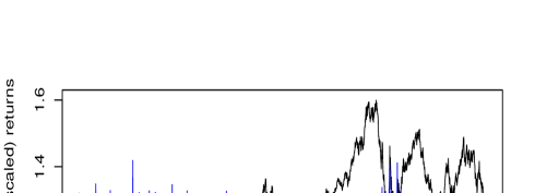
Figure 3: Exchange rate and return USD/EURO, from January 5, 1999 to January 18, 2012.

We also performed out-of-sample predictions of 845 new squared returns, corresponding to the period from January 19, 2012 to May 14, 2015. As loss function we use either $\left(\epsilon_{t}^{2}-\hat{\sigma}_{t}^{2}\right)^{2}$, $\left|\epsilon_{t}^{2}-\hat{\sigma}_{t}^{2}\right|$, $\left(\log\epsilon_{t}^{2}/\hat{\sigma}_{t}^{2}\right)^{2}$, or $\left|\log\epsilon_{t}^{2}/\hat{\sigma}_{t}^{2}\right|$. Averaging over the 845 observations, we obtain respectively the Mean Squared forecast Errors (MSE), the Mean Absolute forecast Errors (MAE), the MSE of the log-squared returns (log-MSE) and the MAE of the log-squared returns (log-MAE). For the volatility prediction $\hat{\sigma}_{t}^{2}$, we used either the Log-GARCH(1,1) or the EGARCH(1,1), both estimated on the initial 3344 observations. Table 7 shows that the Dielbold-Mariano tests (see Dielbold and Mariano (1995)) often reject the null that the two forecasts are equally accurate in average in favor of the alternative that the EGARCH(1,1) produces less accarate forecasts than the Log-GARCH(1,1), except for the CAD series for which the null can not be rejected.

To summarize our empirical investigations, the Log-GARCH(1,1) model seems to be relevant for the USD and GBP series, whereas none of the two models is suitable for the 3 other series.

Table 6: Unrestricted AS-Log-GARCH(1,1) model fitted by QMLE on daily returns of exchange rates.

Currency	$\widehat{\omega}$	$\widehat{\omega}_{-}$	$\widehat{\alpha}_{+}$	$\widehat{\alpha}_{-}$	$\widehat{\beta}$	Log-Lik
USD	-0.008 (0.011)	-0.03 (0.011)	0.022 (0.005)	0.019 (0.005)	0.971 (0.005)	-0.102
JPY	-0.016 (0.017)	-0.121 (0.016)	0.023 (0.006)	0.052 (0.007)	0.949 (0.007)	-0.343
GBP	-0.038 (0.015)	-0.014 (0.016)	0.031 (0.006)	0.027 (0.006)	0.965 (0.006)	-0.547
CHF	-0.135 (0.027)	-0.339 (0.027)	0.003 (0.006)	0.054 (0.007)	0.967 (0.005)	-1.539
CAD	-0.015 (0.011)	-0.011 (0.011)	0.023 (0.005)	0.018 (0.005)	0.970 (0.006)	-0.170

Table 7: $p$-values of the Diebold-Mariano (1995) test for the null that the two models have the same forecast accuracy against the alternative that the EGARCH forecasts are less accurate than those of the Log-GARCH.

	USD	JPY	GBP	CHF	CAD
MSE	0.0410	0.8131	0.6873	0.1070	0.7373
MAE	0.0000	0.0013	0.0322	0.0479	0.1720
Log-MSE	0.0000	0.0012	0.0494	0.0000	0.0702
Log-MAE	0.0000	0.0064	0.1490	0.0000	0.4524

Appendix D Proof of Theorem 4.2

For any $\boldsymbol{\vartheta}=(\boldsymbol{\zeta}^{\prime},\mathbf{0}_{1\times 3q})^{\prime},$ let $\mathbf{T}_{n}({\boldsymbol{\zeta}})=\frac{1}{\sqrt{n}}\sum_{t=1}^{n}\{1-{\eta}_{t}^{2}({\boldsymbol{\zeta}})\}\mathbf{D}_{t}(\boldsymbol{\zeta})$ where ${\mathbf{D}}_{t}(\boldsymbol{\zeta})=\frac{\partial}{\partial\boldsymbol{\alpha}}\log{\sigma}_{t}^{2}(\boldsymbol{\zeta})$ and let $\widetilde{\mathbf{T}}_{n}({\boldsymbol{\zeta}})=\frac{1}{\sqrt{n}}\sum_{t=1}^{n}\{1-\widetilde{\eta}_{t}^{2}({\boldsymbol{\zeta}})\}\widetilde{\mathbf{D}}_{t}({\boldsymbol{\zeta}}),$ where $\eta_{t}(\boldsymbol{\zeta})={\epsilon_{t}}/{{\sigma}_{t}(\boldsymbol{\zeta})}$ and $\widetilde{\eta}_{t}(\boldsymbol{\zeta})={\epsilon_{t}}/{\widetilde{\sigma}_{t}(\boldsymbol{\zeta})}$.

Define

$${\boldsymbol{\cal K}} = \left(\begin{array}[]{cc}{\boldsymbol{\cal K}}_{11}&{\boldsymbol{\cal K}}_{12}\\ {\boldsymbol{\cal K}}_{21}&{\boldsymbol{\cal K}}_{22}\end{array}\right),\quad\mbox{where }\quad{\boldsymbol{\cal K}}_{11}=\mbox{Var}\{\mathbf{D}_{t}(\boldsymbol{\zeta}_{0})\},\quad{\boldsymbol{\cal K}}_{22}=\bf V^{-1}$$

$$\;\;\;\qquad\qquad{\boldsymbol{\cal K}}_{12}={\boldsymbol{\cal K}}_{21}^{\prime}=\mbox{Cov}\{\mathbf{D}_{t}(\boldsymbol{\zeta}_{0}),\nabla\log\sigma_{t}^{2}(\boldsymbol{\zeta}_{0})\}{\bf V}^{-1},$$

and

$${\boldsymbol{\cal L}}={\boldsymbol{\cal K}}_{11}+\boldsymbol{\Psi}{\bf V}^{-1}\boldsymbol{\Psi}^{\prime}+{\boldsymbol{\cal K}}_{12}\boldsymbol{\Psi}^{\prime}+\boldsymbol{\Psi}{\boldsymbol{\cal K}}_{21}$$

where $\boldsymbol{\Psi}=E\{\mathbf{D}_{t}(\boldsymbol{\zeta}_{0})\nabla^{\prime}\log\sigma_{t}^{2}(\boldsymbol{\zeta}_{0})\}.$ Let $\boldsymbol{\Psi}_{i}=E\{\mathbf{D}_{t,i}(\boldsymbol{\zeta}_{0})\nabla^{\prime}\log\sigma_{t}^{2}(\boldsymbol{\zeta}_{0})\}$, where $\mathbf{D}_{t,i}(\boldsymbol{\zeta}_{0})$ denotes the $i$-th component of $\mathbf{D}_{t}(\boldsymbol{\zeta}_{0})$, for $i=1,\ldots 3q$, $t\geq 0$. Let ${\mathbf{T}}_{n,i}(\boldsymbol{\zeta})$ denote the $i$-th component of ${\mathbf{T}}_{n}(\boldsymbol{\zeta})$.

The first step of the proof is similar to the one of the proof of Theorem 3.1. Let $\mathbf{T}_{n,i}$ denote the $i$-th component of $\mathbf{T}_{n}=\widetilde{\mathbf{T}}_{n}(\widehat{\boldsymbol{\zeta}}_{n})$, for $i=1,\ldots 2\ell$. A Taylor expansion gives, for some ${\boldsymbol{\zeta}}_{*}$ between $\widehat{\boldsymbol{\zeta}}_{n}$ and ${\boldsymbol{\zeta}}_{0}$,

$$\mathbf{T}_{n,i}=\widetilde{\mathbf{T}}_{n,i}({\boldsymbol{\theta}}_{0})+\frac{1}{\sqrt{n}}\frac{\partial\widetilde{\mathbf{T}}_{n,i}}{\partial\boldsymbol{\zeta}}({\boldsymbol{\zeta}}_{*})\sqrt{n}(\widehat{\boldsymbol{\zeta}}_{n}-{\boldsymbol{\zeta}}_{0}).$$

We cannot follow the same steps of proof as in Theorem 3.1 because of the lack of moments in the EGARCH(1,1) model for values of $\boldsymbol{\zeta}$ satisfying (4.2), see He et al. (2002). However, using the approach of Straumann and Mikosch (2006) refined in Wintenberger (2013), there exist $K>0$, $\rho\in(0,1)$ and a compact neighborhood ${\cal V}(\boldsymbol{\zeta}_{0})$ such that

$$\sup_{\boldsymbol{\zeta}\in{\cal V}(\boldsymbol{\zeta}_{0})}|\widetilde{\sigma}_{t}^{2}(\boldsymbol{\zeta})-\sigma_{t}^{2}(\boldsymbol{\zeta})|\leq K\rho^{t},\qquad a.s.$$

Moreover, the process $\widetilde{\sigma}_{t}(\boldsymbol{\zeta})$ is lower bounded by $\omega/(1-\beta)>0$ under (4.2). By a Lipschitz argument, we then obtain

$$\sup_{\boldsymbol{\zeta}\in{\cal V}(\boldsymbol{\zeta}_{0})}\left|\frac{1}{\widetilde{\sigma}_{t}^{2}(\boldsymbol{\zeta})}-\frac{1}{\sigma_{t}^{2}(\boldsymbol{\zeta})}\right|\leq K\rho^{t},\quad a.s.$$

By an application of Lemma 2.1 in Straumann and Mikosch (2006), it yields to the first assertion (i) below. It remains to show the three last assertions (ii)-(iv) that are sufficient to prove Theorem 4.2:

$$i)\;\sup_{\boldsymbol{\zeta}\in{\cal V}(\boldsymbol{\zeta}_{0})}\left\|{\mathbf{T}}_{n}(\boldsymbol{\zeta})-\widetilde{\mathbf{T}}_{n}(\boldsymbol{\zeta})\right\|\to 0,\quad\sup_{\boldsymbol{\zeta}\in{\cal V}(\boldsymbol{\zeta}_{0})}\frac{1}{\sqrt{n}}\left\|\frac{\partial{\mathbf{T}}_{n}}{\partial\boldsymbol{\zeta}}(\boldsymbol{\zeta})-\frac{\partial\widetilde{\mathbf{T}}_{n}}{\partial\boldsymbol{\zeta}}(\boldsymbol{\zeta})\right\|\to 0,$$

almost surely,

$$ii)\;\left(\begin{array}[]{c}{\mathbf{T}}_{n}({\boldsymbol{\zeta}}_{0})\\ \sqrt{n}(\widehat{\boldsymbol{\zeta}}_{n}-{\boldsymbol{\zeta}}_{0})\end{array}\right)\stackrel{{\scriptstyle d}}{{\to}}{\cal N}(\mathbf{0},(\kappa_{4}-1){\boldsymbol{\cal K}}),$$

$$iii)\;\frac{1}{\sqrt{n}}\frac{\partial{\mathbf{T}}_{n,i}}{\partial\boldsymbol{\zeta}}(\boldsymbol{\zeta}_{*})\to\boldsymbol{\Psi}_{i},\quad\;\mbox{almost surely, where ${\boldsymbol{\zeta}}_{*}$ is between $\widehat{\boldsymbol{\zeta}}_{n}$ and ${\boldsymbol{\zeta}}_{0}$,}$$

$$v)\;{\boldsymbol{\cal L}}\;\mbox{ is non-singular.}$$

To prove ii), we use that

$$\left(\begin{array}[]{c}{\mathbf{T}}_{n}({\boldsymbol{\zeta}}_{0})\\ \sqrt{n}(\widehat{\boldsymbol{\zeta}}_{n}-{\boldsymbol{\zeta}}_{0})\end{array}\right)=\frac{1}{\sqrt{n}}\sum_{t=1}^{n}(1-{\eta}_{t}^{2})\left(\begin{array}[]{c}\mathbf{D}_{t}(\boldsymbol{\zeta}_{0})\\ -{\bf V}^{-1}\nabla\log\sigma_{t}^{2}(\boldsymbol{\zeta}_{0})\end{array}\right)+o_{P}(1).$$

The convergence in distribution thus follows from the central limit theorem for martingale differences.

The proof of iii) relies on an almost sure uniform argument applied to $\partial{\mathbf{T}}_{n}/\partial\boldsymbol{\zeta}(\boldsymbol{\zeta})$ on some neighborhood of $\boldsymbol{\zeta}_{0}$. As $\boldsymbol{\zeta}_{\ast}$ converges almost surely to $\boldsymbol{\zeta}_{0}$, step i) ensures that

$$\frac{1}{\sqrt{n}}\left|\frac{\partial{\mathbf{T}}_{n}}{\partial\boldsymbol{\zeta}}(\boldsymbol{\zeta}_{\ast})-\frac{\partial\widetilde{\mathbf{T}}_{n}}{\partial\boldsymbol{\zeta}}(\boldsymbol{\zeta}_{0})\right|\to 0\qquad a.s.$$

Thus, the result will follow from the ergodic theorem applied to $(\nabla{\bf T}_{n}(\boldsymbol{\zeta}_{0}))$ if ${\bf\Psi}$ is finite. Indeed, the linear stochastic recurrent equation (4.3) when $\boldsymbol{\zeta}=\boldsymbol{\zeta}_{0}$ takes a simple form with a Lipschitz coefficient equals to $\beta_{0}-\frac{1}{2}(\gamma_{0}\eta_{t}+\delta_{0}|\eta_{t}|)$. Under A9, one can use a contractive argument in $L^{2}$ to prove that $E\{{\bf D}_{t,i}(\boldsymbol{\zeta}_{0})^{2}\}<\infty$, $i=1,\ldots,3q$. The same argument was already used in Wintenberger (2013) to prove that $E\{\nabla^{\prime}\log\sigma_{t}^{2}(\boldsymbol{\zeta}_{0})\nabla\log\sigma_{t}^{2}(\boldsymbol{\zeta}_{0})\}<\infty$. Thus, the finiteness of ${\bf\Psi}_{i}$ is derived from the Cauchy-Schwarz inequality and step iii) follows.

Let us prove step iv). Suppose there exist ${\bf x}=(x_{i})\in\mathbb{R}^{3q}$ and ${\bf y}\in\mathbb{R}^{4}$ such that

$${\bf x}^{\prime}\mathbf{D}_{t}(\boldsymbol{\zeta}_{0})+{\bf y}^{\prime}{\bf V}^{-1}\nabla\log\sigma_{t}^{2}(\boldsymbol{\zeta}_{0})=0.$$ (D.4)

Let ${\bf z}^{\prime}={\bf y}^{\prime}{\bf V}^{-1}$. In view of (4.3) we have

$$\nabla\log\sigma_{t}^{2}(\boldsymbol{\zeta}_{0}) = {U}_{t-1}(\boldsymbol{\zeta}_{0})\nabla\log\sigma_{t-1}^{2}(\boldsymbol{\zeta}_{0})+\left(1,\epsilon_{t-1},|\epsilon_{t-1}|,\log\sigma_{t-1}^{2}(\boldsymbol{\zeta}_{0})\right)^{\prime},$$

$${\mathbf{D}}_{t}(\boldsymbol{\zeta}_{0}) = {U}_{t-1}(\boldsymbol{\zeta}_{0}){\mathbf{D}}_{t-1}(\boldsymbol{\zeta}_{0})+\left({\bf 1}_{t-1,q}^{-^{\prime}},\boldsymbol{\epsilon}_{t-1,q}^{+^{\prime}},\boldsymbol{\epsilon}_{t-1,q}^{-^{\prime}}\right)^{\prime}.$$

By stationarity, it follows from (D.4) that

$$\boldsymbol{x}^{\prime}\left({\bf 1}_{t-1,q}^{-},\boldsymbol{\epsilon}_{t-1,q}^{+},\boldsymbol{\epsilon}_{t-1,q}^{-}\right)^{\prime}+\boldsymbol{z}^{\prime}\left(1,\epsilon_{t-1},|\epsilon_{t-1}|,\log\sigma_{t-1}^{2}(\boldsymbol{\zeta}_{0})\right)^{\prime}=0,\quad a.s.$$ (D.5)

It follows that, with notations already used,

$$x_{1}1_{\{\eta_{t-1}<0\}}+x_{q+1}\log\epsilon_{t-1}^{2}1_{\{\eta_{t-1}<0\}}+x_{2q+1}\log\epsilon_{t-1}^{2}1_{\{\eta_{t-1}>0\}}$$

$$+z_{1}+z_{2}\eta_{t-1}\sigma_{t-1}(\boldsymbol{\zeta}_{0})+z_{3}|\eta_{t-1}|\sigma_{t-1}(\boldsymbol{\zeta}_{0})+z_{4}\log\sigma_{t-1}^{2}(\boldsymbol{\zeta}_{0}) = R_{t-2}.$$ (D.6)

Thus, conditioning on $\eta_{t-1}<0$ we find

$$x_{1}+x_{q+1}\log\eta_{t-1}^{2}+z_{1}+(z_{2}+z_{3})\eta_{t-1}\sigma_{t-1}(\boldsymbol{\zeta}_{0})+(z_{4}+x_{q+1})\log\sigma_{t-1}^{2}(\boldsymbol{\zeta}_{0}) = R_{t-2}.$$

By arguments already used, in view of Assumption A8 this entails $x_{q+1}=z_{2}+z_{3}=0$. By conditioning on $\eta_{t-1}>0$ we find $x_{2q+1}=z_{2}-z_{3}=0$ and (D) reduces to

$$x_{1}1_{\{\eta_{t-1}<0\}}+z_{1}+z_{4}\log\sigma_{t-1}^{2}(\boldsymbol{\zeta}_{0}) = R_{t-2}.$$

The sign of $\eta_{t-1}$ being independent of $\sigma\left(\{\eta_{u},u\leq t-2\}\right)$ we also have $x_{1}=0$. Turning back to (D), we get $x_{2}1_{\{\eta_{t-2}<0\}}+x_{q+2}\log\epsilon_{t-2}^{2}1_{\{\eta_{t-2}>0\}}+x_{2q+2}\log\epsilon_{t-2}^{2}1_{\{\eta_{t-2}<0\}}+z_{1}+z_{4}\log\sigma_{t-1}^{2}(\boldsymbol{\zeta}_{0})=R_{t-3}.$ Because $\log\sigma_{t-1}^{2}(\boldsymbol{\zeta}_{0})=\omega_{0}+\gamma_{0}\eta_{t-2}+\delta_{0}|\eta_{t-2}|+\beta_{0}\log\sigma_{t-2}^{2}(\boldsymbol{\zeta}_{0})$ we get, for $\eta_{t-2}<0$,

$$x_{2}+x_{2q+2}\log\eta_{t-2}^{2}+z_{1}+z_{4}(\omega_{0}+(\gamma_{0}-\delta_{0})\eta_{t-2}) = R_{t-3}^{*}.$$

By arguments already used, we deduce that $x_{2q+2}=z_{4}=0$. By conditioning on $\eta_{t-2}>0$, we get $x_{q+2}=0$ and thus $x_{2}=0$. Proceeding similarly we show that all the components of $\boldsymbol{x}$ are equal to zero. Using (D.5), we thus have $z_{1}=0$. We have shown that, in (D.4), $\boldsymbol{x}=\boldsymbol{0}$ and $\boldsymbol{y}=\boldsymbol{0}$ which entails that ${\boldsymbol{\cal L}}$ is non-singular. $\Box$

Appendix E Proof of Theorem 5.1

Introduce the vector $\boldsymbol{r}_{m}=\left(r_{1},\dots,r_{m}\right)^{\prime}$ where

$$r_{h}=n^{-1}\sum_{t=h+1}^{n}s_{t}s_{t-h},\qquad\mbox{ with }s_{t}=\eta_{t}^{2}-1\mbox{ and }0<h<n.$$

Let $s_{t}(\boldsymbol{\theta})$ (respectively $\widetilde{s}_{t}(\boldsymbol{\theta})$) be the random variable obtained by replacing $\eta_{t}$ by $\eta_{t}(\boldsymbol{\theta})=\epsilon_{t}/\sigma_{t}(\boldsymbol{\theta})$ (respectively $\widetilde{\eta}_{t}(\boldsymbol{\theta})=\epsilon_{t}/\widetilde{\sigma}_{t}(\boldsymbol{\theta})$) in $s_{t}$. Let $r_{h}(\boldsymbol{\theta})$ (respectively $\widetilde{r}_{h}(\boldsymbol{\theta})$) be obtained by replacing $\eta_{t}$ by $\eta_{t}(\boldsymbol{\theta})$ (respectively $\widetilde{\eta}_{t}(\boldsymbol{\theta})$) in $r_{h}$. The vectors $\boldsymbol{r}_{m}(\boldsymbol{\theta})=\left(r_{1}(\boldsymbol{\theta}),\dots,r_{m}(\boldsymbol{\theta})\right)^{\prime}$ and $\boldsymbol{\widetilde{r}}_{m}(\boldsymbol{\theta})=\left(\boldsymbol{\widetilde{r}}_{1}(\boldsymbol{\theta}),\dots,\boldsymbol{\widetilde{r}}_{m}(\boldsymbol{\theta})\right)^{\prime}$ are such that $\boldsymbol{r}_{m}=\boldsymbol{r}_{m}(\boldsymbol{\theta}_{0})$ and $\boldsymbol{\widehat{r}}_{m}=\boldsymbol{\widetilde{r}}_{m}(\widehat{\boldsymbol{\theta}}_{n})$.

We first study the asymptotic impact of the unknown initial values on the statistic $\boldsymbol{\widehat{r}}_{m}$. We have $s_{t}(\boldsymbol{\theta})s_{t-h}(\boldsymbol{\theta})-\widetilde{s}_{t}(\boldsymbol{\theta})\widetilde{s}_{t-h}(\boldsymbol{\theta})=a_{t}+b_{t}$ with $a_{t}=\left\{s_{t}(\boldsymbol{\theta})-\widetilde{s}_{t}(\boldsymbol{\theta})\right\}s_{t-h}(\boldsymbol{\theta})$ and $b_{t}=\widetilde{s}_{t}(\boldsymbol{\theta})\left\{s_{t-h}(\boldsymbol{\theta})-\widetilde{s}_{t-h}(\boldsymbol{\theta})\right\}$. A straightforward adaptation of the proof of (3.7) shows that the right-hand side can be replaced by $K\rho^{t}$ in this inequality. Thus, we have

$$\left|a_{t}\right| \leq K\rho^{t}\epsilon_{t}^{2}\left(\frac{\sigma_{t-h}^{2}}{\sigma_{t-h}^{2}(\boldsymbol{\theta})}\eta_{t-h}^{2}+1\right).$$

Lemma 3.1 and the $c_{r}$ and H lder inequalities entail that for sufficiently small $s^{*}\in(0,1)$, there exists a neighborhood $\mathcal{V}$ of $\boldsymbol{\theta}_{0}$ such that

$$E\left|\frac{1}{\sqrt{n}}\sum_{t=1}^{n}\sup_{\boldsymbol{\theta}\in\mathcal{V}}|a_{t}|\right|^{s^{*}}\leq Kn^{-s^{*}/2}\sum_{t=1}^{n}\rho^{ts^{*}}\to 0$$

as $n\to\infty$. It follows that $n^{-1/2}\sum_{t=1}^{n}\sup_{\boldsymbol{\theta}\in\mathcal{V}}|a_{t}|=o_{P}(1)$. The same convergence holds for $b_{t}$ and for the derivatives of $a_{t}$ and $b_{t}$. We then obtain

$$\sqrt{n}\left\|\boldsymbol{r}_{m}-\widetilde{r}_{m}(\boldsymbol{\theta}_{0})\right\|=o_{P}(1),\qquad\sup_{\boldsymbol{\theta}\in\mathcal{V}}\left\|\nabla\boldsymbol{r}^{\prime}_{m}(\boldsymbol{\theta})-\nabla\boldsymbol{\widetilde{r}}^{\prime}_{m}(\boldsymbol{\theta})\right\|=o_{P}(1).$$ (E.1)

We now show that the asymptotic distribution of $\sqrt{n}\boldsymbol{\widehat{r}}_{m}$ is a function of the joint asymptotic distribution of $\sqrt{n}\boldsymbol{r}_{m}$ and of the QMLE. Using (E.1) and the consistency of $\widehat{\boldsymbol{\theta}}_{n}$, Taylor expansions of the components of $\boldsymbol{r}_{m}(\cdot)$ around $\widehat{\boldsymbol{\theta}}_{n}$ and $\boldsymbol{\theta}_{0}$ shows that

$$\sqrt{n}\boldsymbol{\widehat{r}}_{m} = \sqrt{n}\boldsymbol{\widetilde{r}}_{m}(\boldsymbol{\theta}_{0})+\left[\nabla{\widetilde{\boldsymbol{r}}}^{\prime}_{m}(\boldsymbol{\theta}^{*})\right]^{\prime}\sqrt{n}(\widehat{\boldsymbol{\theta}}_{n}-\boldsymbol{\theta}_{0})$$

$$= \sqrt{n}\boldsymbol{r}_{m}+\left[\nabla{\boldsymbol{r}}^{\prime}_{m}(\boldsymbol{\theta}^{*})\right]^{\prime}\sqrt{n}(\widehat{\boldsymbol{\theta}}_{n}-\boldsymbol{\theta}_{0})+o_{P}(1)$$

where the $h$-th row of the matrix $\left[\nabla{\widetilde{\boldsymbol{r}}}^{\prime}_{m}(\boldsymbol{\theta}^{*})\right]^{\prime}$ is the transpose of $\nabla\widetilde{r}_{h}(\boldsymbol{\theta}_{h}^{*})$ for some $\boldsymbol{\theta}_{h}^{*}$ between $\widehat{\boldsymbol{\theta}}_{n}$ and $\boldsymbol{\theta}_{0}$. In Section 7.11 of FWZ, we have shown the existence of moments of all order for $\log\sigma_{t}^{2}(\boldsymbol{\theta})$ and their derivatives at any order, uniformly in $\boldsymbol{\theta}\in{\cal V}$ for some neighborhood ${\cal V}$ of $\boldsymbol{\theta}_{0}$. Together with Lemma 3.1, this implies that

$$E\sup_{\boldsymbol{\theta}\in{\cal V}}\left|\frac{\partial^{2}s_{t}(\boldsymbol{\theta})s_{t-h}(\boldsymbol{\theta})}{\partial\boldsymbol{\theta}_{i}\partial\boldsymbol{\theta}_{j}}\right|<\infty\quad\mbox{for all }i,j\in\{1,\dots,d\}.$$

Using these inequalities, the assumption $E\eta_{t}^{4}<\infty$, and the almost sure convergence of $\boldsymbol{\theta}_{h}^{*}$ to $\boldsymbol{\theta}_{0}$, Taylor expansions and the ergodic theorem yield

$$\nabla r_{h}(\boldsymbol{\theta}_{h}^{*})=\nabla r_{h}(\boldsymbol{\theta}_{0})+o_{P}(1)\to c_{h}:=E\left\{s_{t-h}\nabla s_{t}(\boldsymbol{\theta}_{0})\right\}=-E\left\{s_{t-h}\nabla\log\sigma_{t}^{2}(\boldsymbol{\theta}_{0})\right\}.$$

Note that $c_{h}$ is the almost sure limit of (5.1). Let $\boldsymbol{K}_{m}$ be the $m\times d$ matrix whose $h$-th row is $c_{h}^{\prime}$. We have shown that

$$\sqrt{n}\boldsymbol{\widehat{r}}_{m}=\sqrt{n}\boldsymbol{r}_{m}+\boldsymbol{K}_{m}\sqrt{n}(\widehat{\boldsymbol{\theta}}_{n}-\boldsymbol{\theta}_{0})+o_{P}(1).$$ (E.2)

We now derive the asymptotic distribution of $\sqrt{n}(\boldsymbol{r}_{m},\widehat{\boldsymbol{\theta}}_{n}-\boldsymbol{\theta}_{0})$. Note that

$$\boldsymbol{r}_{m}=\frac{1}{n}\sum_{t=1}^{n}s_{t}\boldsymbol{s}_{t-1:t-m}+o_{P}(1)\quad\mbox{where}\quad\boldsymbol{s}_{t-1:t-m}=(s_{t-1},\dots,s_{t-m})^{\prime}.$$

With this notation, we have $\boldsymbol{K}_{m}=-E\boldsymbol{s}_{t-1:t-m}\nabla^{\prime}\log\sigma_{t}^{2}(\boldsymbol{\theta}_{0})$. We have seen in the proof of Theorem 3.1 that

$$\sqrt{n}\left(\widehat{\boldsymbol{\theta}}_{n}-\boldsymbol{\theta}_{0}\right)=-\boldsymbol{J}^{-1}\frac{1}{\sqrt{n}}\sum_{t=1}^{n}(1-\eta^{2}_{t})\nabla\log\sigma_{t}^{2}(\boldsymbol{\theta}_{0})+o_{P}(1).$$

The central limit theorem applied to the martingale difference

$$\left\{\left(s_{t}\nabla^{\prime}\log\sigma_{t}^{2}(\boldsymbol{\theta}_{0}),s_{t}\boldsymbol{s}_{t-1:t-m}^{\prime}\right)^{\prime};\sigma\left(\eta_{u},\,u\leq t\right)\right\}$$

then shows that

$$\sqrt{n}\left(\begin{array}[]{c}\widehat{\boldsymbol{\theta}}_{n}-\boldsymbol{\theta}_{0}\\ \boldsymbol{r}_{m}\end{array}\right) = \frac{1}{\sqrt{n}}\sum_{t=1}^{n}s_{t}\left(\begin{array}[]{c}\boldsymbol{J}^{-1}\nabla\log\sigma_{t}^{2}(\boldsymbol{\theta}_{0})\\ \boldsymbol{s}_{t-1:t-m}\end{array}\right)+o_{P}(1)$$ (E.7)

$$\stackrel{{\scriptstyle\boldsymbol{\cal L}}}{{\to}} {\cal N}\left\{\boldsymbol{0},\left(\begin{array}[]{cc}(\kappa_{4}-1)\boldsymbol{J}^{-1}&\boldsymbol{\Sigma}_{\widehat{\boldsymbol{\theta}}_{n}\boldsymbol{r}_{m}}\\ \boldsymbol{\Sigma}_{\widehat{\boldsymbol{\theta}}_{n}\boldsymbol{r}_{m}}^{\prime}&(\kappa_{4}-1)^{2}\boldsymbol{I}_{m}\end{array}\right)\right\},$$ (E.10)

where

$$\boldsymbol{\Sigma}_{\widehat{\boldsymbol{\theta}}_{n}\boldsymbol{r}_{m}} = (\kappa_{4}-1)\boldsymbol{J}^{-1}E\nabla\log\sigma_{t}^{2}(\boldsymbol{\theta}_{0})\boldsymbol{s}_{t-1:t-m}^{\prime}=-(\kappa_{4}-1)\boldsymbol{J}^{-1}\boldsymbol{K}_{m}^{\prime}.$$

Using together (E.2) and (E.7), we obtain

$$\sqrt{n}\boldsymbol{\widehat{r}}_{m} \stackrel{{\scriptstyle\boldsymbol{\cal L}}}{{\to}} {\cal N}\left(\boldsymbol{0},\boldsymbol{D}\right),\quad\boldsymbol{D}=(\kappa_{4}-1)^{2}\boldsymbol{I}_{m}-(\kappa_{4}-1)\boldsymbol{K}_{m}\boldsymbol{J}^{-1}\boldsymbol{K}_{m}^{\prime}.$$

We now show that $\boldsymbol{D}$ is invertible. Assumption A3 entails that the law of $\eta_{t}^{2}$ is non degenerated. We thus have $\kappa_{4}>1$, and it remains to show the invertibility of

$$(\kappa_{4}-1)\boldsymbol{I}_{m}-\boldsymbol{K}_{m}\boldsymbol{J}^{-1}\boldsymbol{K}_{m}^{\prime}=E\mathbf{V}\mathbf{V}^{\prime},\quad\mathbf{V}=\boldsymbol{s}_{-1:-m}+\boldsymbol{K}_{m}\boldsymbol{J}^{-1}\nabla\log\sigma_{0}^{2}(\boldsymbol{\theta}_{0}).$$

If this matrix were singular then there would exist $\boldsymbol{\lambda}=(\lambda_{1},\dots,\lambda_{m})^{\prime}$ such that $\boldsymbol{\lambda}\neq\boldsymbol{0}$ and

$$\boldsymbol{\lambda}^{\prime}\mathbf{V}=\boldsymbol{\lambda}^{\prime}\boldsymbol{s}_{-1:-m}+\boldsymbol{\mu}^{\prime}\nabla\log\sigma_{0}^{2}(\boldsymbol{\theta}_{0})=\boldsymbol{0}\quad\mbox{ a.s.,}$$ (E.11)

with $\boldsymbol{\mu}^{\prime}=\boldsymbol{\lambda}^{\prime}\boldsymbol{K}_{m}\boldsymbol{J}^{-1}$. Note that

$$\nabla\log\sigma_{t}^{2}(\boldsymbol{\theta})=\sum_{j=1}^{p}\beta_{j}\nabla\log\sigma^{2}_{t-j}(\boldsymbol{\theta})+\left(1,{\bf 1}_{t-1,q}^{-}\\ \boldsymbol{\epsilon}_{t-1,q}^{+},\boldsymbol{\epsilon}_{t-1,q}^{-},\boldsymbol{\sigma}^{2}_{t-1,p}(\boldsymbol{\theta})\right)^{\prime},$$ (E.12)

Equation (E.11) gives

$$\boldsymbol{\lambda}^{\prime}\mathbf{V}=\lambda_{1}\eta^{2}_{-1}+\mu_{2}1_{\eta_{-1}<0}+\mu_{2+q}1_{\eta_{-1}>0}\log\epsilon^{2}_{-1}+\mu_{2+2q}1_{\eta_{-1}<0}\log\epsilon^{2}_{-1}+R_{-2}.$$ (E.13)

Thus (E.11) entails the two equations

$$1_{\eta_{-1}>0}\left\{\lambda_{1}\eta^{2}_{-1}+\mu_{2+q}\log\eta^{2}_{-1}+R_{-2}\right\}=0\quad\mbox{ a.s.}$$ (E.14)

and

$$1_{\eta_{-1}<0}\left\{\lambda_{1}\eta^{2}_{-1}+\mu_{2+2q}\log\eta^{2}_{-1}+R_{-2}\right\}=0\quad\mbox{ a.s.}$$ (E.15)

Note that an equation of the form $ax^{2}+b\log|x|+c=0$ cannot have more than 2 positive roots or more than 2 negative roots, except if $a=b=c=0$. By Assumption A10, Equations (E.14) and (E.15) thus imply $\lambda_{1}=0$. We thus also have $\mu_{2+q}=\mu_{2+2q}=0$ and it follows from (E.13) that $\mu_{2}=0$. Given that $\lambda_{1}=\mu_{2}=\mu_{2+q}=\mu_{2+2q}=0$, (E.11) and (E.12) now give

$$\boldsymbol{\lambda}^{\prime}\mathbf{V} = \lambda_{2}\eta^{2}_{-2}+\mu_{3}1_{\eta_{-2}<0}+\mu_{3+q}1_{\eta_{-2}>0}\log\epsilon^{2}_{-2}+\mu_{3+2q}1_{\eta_{-2}<0}\log\epsilon^{2}_{-2}$$ (E.16)

$$+\mu_{3+3q}\log\sigma^{2}_{-1}+R_{-3}=0.$$

Since

$$\log\sigma^{2}_{-1} = \omega+\omega_{1-}R_{-3}1_{\eta_{-2}<0}+\alpha_{1+}1_{\eta_{-2}>0}(\log\eta^{2}_{-2}+R_{-3})$$

$$+\alpha_{1-}1_{\eta_{-2}<0}(\log\eta^{2}_{-2}+R_{-3})+R_{-3},$$

we have the two equations

$$1_{\eta_{-2}>0}\left\{\lambda_{2}\eta^{2}_{-2}+(\mu_{3+q}+\mu_{3+3q}\alpha_{1+})\log\eta^{2}_{-2}+R_{-3}\right\}=0\quad\mbox{ a.s.}$$

and

$$1_{\eta_{-2}<0}\left\{\lambda_{2}\eta^{2}_{-2}+(\mu_{3+2q}+\mu_{3+3q}\alpha_{1-})\log\eta^{2}_{-2}+R_{-3}\right\}=0\quad\mbox{ a.s.}$$

By Assumption A10, we obtain

$$\lambda_{2}=\mu_{3+q}+\mu_{3+3q}\alpha_{1+}=\mu_{3+2q}+\mu_{3+3q}\alpha_{1-}=0.$$

In view of (E.16), it follows that $\mu_{3}=0$. By iterating the previous arguments, it can be shown that $\lambda_{1}=\cdots=\lambda_{m}=0$ which leads to a contradiction. The non-singularity of $\boldsymbol{D}$ follows. The proof of the convergence $\widehat{\boldsymbol{D}}\to\boldsymbol{D}$ in probability (and even almost surely) as $n\to\infty$ is omitted. $\Box$

References

[1] Berkes, I., Horváth, L. and P. Kokoszka (2003)
GARCH processes: structure and estimation. Bernoulli 9,
201–227.
[2] Box, G.E.P. and D.A. Pierce (1970) Distribution of the residual autocorrelations in
autoregressive-integrated moving average time series models. Journal of the American
Statistical Association 65, 1509–1526.
[3] Carbon, M. and C. Francq (2011) Portmanteau goodness-of-fit test for asymmetric power GARCH models. Austrian Journal of Statistics 40, 55–64.
[4] Escanciano, J.C. (2010) Asymptotic distribution-free diagnostic tests for heteroskedastic time series models. Econometric Theory 26, 744–773.
[5] Francq, C., L. Horváth and J.M. Zako an (2010) Sup-tests for linearity in a general nonlinear AR(1) model.
Econometric Theory 26, 965–993.
[6] Francq, C., Wintenberger, O. and J.M. Zako an (2013)
GARCH models without positivity constraints: Exponential or Log
GARCH? Journal of Econometrics 177, 34–46.
[7] Francq, C. and Zako an, J-M. (2011)
QML estimation of a class of multivariate asymmetric GARCH models.
Econometric Theory 28, 1–28.
[8] Geweke, J. (1986) Modeling the persistence of conditional variances: A Comment. Econometric
Review 5, 57–61.
[9] Harvey, A. C. and Sucarrat, G. (2014) EGARCH models with fat tails, skewness and leverage.
Computational Statistics and Data Analysis 76, 320–338.
[10] He, C., Teräsvirta, T. and Malmsten, H. (2002) Moment structure of a family of first-order exponential GARCH models. Econometric Theory 18, 868–885.
[11] Leucht, A., Kreiss, J-P. and M. Neumann (2015) A model specification test for GARCH(1,1) processes.
Scandinavian Journal of Statistics 42, 1167–1193.
[12] Li, W.K. (2004) Diagnostic checks in time series. Boca Raton, Florida: Chapman and
Hall.
[13] Li, W.K. and T.K. Mak (1994) On the squared residual autocorrelations in non-linear time series
with conditional heteroscedasticity. Journal of Time Series Analysis 15, 627–636.
[14] Ling, S. and W.K. Li (1997). On fractionally integrated autoregressive moving-average
time series models with conditional heteroscedasticity. Journal of the American
Statistical Association 92, 1184–1194.
[15] Ljung, G.M. and G.E.P. Box (1978) On the measure of lack of fit in time series models.
Biometrika 65, 297–303.
[16] Luukkonen, R., Saikkonen, P., and T. Teräsvirta (1988) Testing linearity against smooth
transition autoregressive models. Biometrika, 75, 491–499.
[17] McLeod, A.I. (1978) On the distribution of residual autocorrelations in Box-Jenkins
method. Journal of the Royal Statistical Society B 40, 296–302.
[18] Milh j, A. (1987) A Multiplicative Parameterization of ARCH Models. Working paper, Department
of Statistics, University of Copenhagen.
The Power Log-GARCH model
[19] Nelson D.B. (1991)
Conditional Heteroskedasticity in Asset Returns : a New
Approach. Econometrica 59, 347–370.
[20] Pantula, S.G. (1986) Modeling the Persistence of Conditional Variances: A Comment. Econometric
Review 5, 71–74.
[21] Sucarrat, G., Gr nneberg, S. and A. Escribano (2015)
Estimation and Inference in Univariate and Multivariate Log-GARCH-X Models When the Conditional Density is Unknown. Forthcoming in Computational Statistics and Data Analysis.
[22] Straumann, D. and Mikosch, T. (2006)
Quasi-maximum likelihood estimation in conditionally heteroscedastic
time series: a stochastic recurrent equations approach. Ann. Statist. 34, 2449–2495.
[23] Wintenberger, O. (2013)
Continuous Invertibility and Stable QML Estimation of the EGARCH(1,1) Model. Scandinavian Journal of Statistics 40, 846–867.

References

[1] Diebold, F.X. and R.S. Mariano (1995) Comparing Predictive Accuracy. Journal of Business and Economic Statistics 13, 253–263.