Probing the magnetic field structure in Sgr A^∗ on Black Hole Horizon Scales with Polarized Radiative Transfer Simulations

Abstract

Magnetic fields are believed to drive accretion and relativistic jets in black hole accretion systems, but the magnetic-field structure that controls these phenomena remains uncertain. We perform general relativistic (GR) polarized radiative transfer of time-dependent three-dimensional GR magnetohydrodynamical (MHD) simulations to model thermal synchrotron emission from the Galactic Center source Sagittarius A^∗ (Sgr A^∗). We compare our results to new polarimetry measurements by the Event Horizon Telescope (EHT) and show how polarization in the visibility (Fourier) domain distinguishes and constrains accretion flow models with different magnetic field structures. These include models with small-scale fields in disks driven by the magnetorotational instability (MRI) as well as models with large-scale ordered fields in magnetically-arrested disks (MAD). We also consider different electron temperature and jet mass-loading prescriptions that control the brightness of the disk, funnel-wall jet, and Blandford-Znajek-driven funnel jet. Our comparisons between the simulations and observations favor models with ordered magnetic fields near the black hole event horizon in Sgr A^∗, although both disk- and jet-dominated emission can satisfactorily explain most of the current EHT data. We show that stronger model constraints should be possible with upcoming circular polarization and higher frequency ($349~{}{\rm GHz}$) measurements.

1. Introduction

The origin of the radio emission of Sgr A^∗ has been the subject of intense observational studies (Falcke et al., 1998; Reid, 2009; Doeleman et al., 2008; Dodds-Eden et al., 2009) and theoretical modeling (Narayan & Yi, 1994; Yuan et al., 2002; Dexter et al., 2009; Mościbrodzka et al., 2009; Penna et al., 2010; Mościbrodzka et al., 2012; Mościbrodzka & Falcke, 2013; Mościbrodzka et al., 2014). Near-infrared observations (Genzel et al., 2010) of stars orbiting an unseen central mass so-far provide the most direct evidence for the existence of a black hole (BH) and yield a BH mass of $M=4.5\pm 0.4\times 10^{6}{\rm M_{\odot}}$ (Ghez et al., 2008). Observations covering a wide range of the electromagnetic spectrum rule out a standard thin disk model and clearly reveal that Sgr A^∗ is highly underluminous (compared to its Eddington limit), presumably due to a highly sub-Eddington accreting BH (Falcke et al., 1998; Reid, 2009; Dodds-Eden et al., 2009). This regime of the accretion disk has been studied extensively (Yuan & Narayan, 2014) and features a hot, magnetized accretion flow composed of a weakly collisional plasma. Synchrotron emission is the main contribution to the near-mm flux due the low density and dynamically important magnetic fields. The unresolved (“zero-baseline”) flux has been measured in radio (Falcke et al., 1998; Bower et al., 2015), infrared (Schödel et al., 2011), and X-ray (Baganoff et al., 2003) and exhibits diverse phenomena, such as flaring in the near-infrared (Genzel et al., 2003; Yuan et al., 2004; Eckart et al., 2006a) and X-rays (Eckart et al., 2006b).

Very-long baseline interferometric (VLBI) radio measurements, such as those with the Event Horizon Telescope (EHT) (Doeleman et al., 2009), offer an unprecedented capability to identify the physics near a rotating BH in Sgr A^∗ due to the EHT’s high observing frequency (230 GHz), resolving power, and sensitivity. Recently, VLBI observations with the EHT have determined the correlated flux density of Sgr A^∗ (and M87) on VLBI baselines, thereby partially resolving the emission structure and constraining the size of the emitting region (Doeleman et al., 2008; Fish et al., 2011; Doeleman et al., 2012; Akiyama et al., 2015; Johnson et al., 2015b). The EHT probes the strong field regime of GR and may be capable of detecting the BH’s shadow (Bardeen, 1973; Luminet, 1979; Falcke et al., 2000; Dexter et al., 2010; Fish et al., 2014; Psaltis et al., 2015).

The EHT can also resolve polarized structure on event horizon scales, which may allow one to distinguish between competing models of accretion disks and jets. Whether a jet is launched depends upon the BH spin, structure of the magnetic field threading the disk and BH, and the mass-loading of the polar magnetic field (Blandford & Znajek, 1977; Komissarov & McKinney, 2007). If the magnetic field structure consists of small-scale MHD turbulence driven by the magnetorotational instability (MRI) (Balbus & Hawley, 1998), then the production of a jet is either not possible due to rapid reconnection of a disorganized magnetic field (Beckwith et al., 2008; McKinney & Blandford, 2009) or is at least difficult without a collisional ideal MHD plasma (McKinney & Uzdensky, 2012; McKinney et al., 2012). Some researchers call such MRI-driven disks a type of standard-and-normal-evolution (SANE) accretion flow (Narayan et al., 2012). In another limit, a plentiful supply of ordered vertical magnetic flux builds-up near the BH until reaching saturation, in which case the MRI is marginally suppressed and the disk enters the so-called magnetically arrested disk (MAD) state driven by magnetic Rayleigh-Taylor instabilities (Narayan et al., 2003; Igumenshchev et al., 2003; Tchekhovskoy et al., 2011; McKinney et al., 2012).

Time-dependent global general relativistic magnetohydrodynamical (GRMHD) simulations of a variety of BH accretion flow types are essential to understand the possible range of disk and jet states and their underlying dynamics. A significant theoretical uncertainty in modeling Sgr A^∗ is that such weakly collisional flows involve kinetic physics with undetermined heating rates (Quataert & Gruzinov, 1999; Sharma et al., 2006; Johnson & Quataert, 2007; Howes et al., 2008; Riquelme et al., 2012, 2015) for a population of thermal or non-thermal electrons (Mahadevan & Quataert, 1997; Özel et al., 2000; Yuan et al., 2003; Lynn et al., 2014) not fully accounted for in GRMHD simulations. For example, the jet might light-up only if actually launched under favorable physical conditions, or the jet could be always present but the particle heating could control whether the jet lights up. Relativistic jets are commonly invoked to interpret the emission from compact radio sources (Blandford & Königl, 1979). In particular, for Sgr A^∗ and M87, jet models have been successfully applied to explain the spectral energy distribution (SED) with certain assumptions about the electron temperatures (Falcke & Markoff, 2000; Doeleman et al., 2012). While no clear unambiguous spectral or imaging signature of such a jet has been found in Sgr A^∗(frequency-dependent light curves show time-lagged correlations indicative of expansion or outflows (Marrone et al., 2008; Yusef-Zadeh et al., 2008; Brinkerink et al., 2015)), evidence for or against jets could come from polarimetric observations that depend upon the nature of the magnetic field.

There is also theoretical uncertainty in the amount of particles that should be present inside Blandford & Znajek (1977) (hereafter BZ) driven jets. GRMHD numerical simulations with BZ-driven jets must inject matter in some way to keep the numerical scheme stable (Gammie et al., 2003). In real astrophysical systems, the nature of mass-loading of jets remains uncertain and could be due to photon annihilation or pair cascades to some degree for Sgr A^∗ (Mościbrodzka et al., 2011), but this creates only a low-level of mass-loading (much lower than GRMHD numerical schemes can handle). In some cases, like for Sgr A^∗, the level of mass-loading might even be insufficient to enable force-free or MHD conditions in the highly-magnetized funnel (Levinson et al., 2005; Broderick & Tchekhovskoy, 2015). MHD dynamical mass-loading due to magnetic Rayleigh-Taylor instabilities at the disk-jet interface might lead to significant mass-loading, which could depend upon the disk type, with MADs generating more mass-loading due to large-scale magnetic oscillations that connect the disk and jet (McKinney et al., 2012). However, no work has yet quantified such an MHD-based mass-loading mechanism.

Accounting for these various uncertainties, GRMHD simulations can then be used as dynamical models in a radiative transfer calculation in order to compare with observations (Dexter et al., 2009; Mościbrodzka et al., 2009; Dexter et al., 2010; Shcherbakov et al., 2012a; Mościbrodzka et al., 2014; Chan et al., 2015a, b). In particular, polarized radiative transfer offers up to four times the information of unpolarized studies (Shcherbakov & Huang, 2011; Shcherbakov et al., 2012a), potentially leading to much better constraints on models and theories of accretion flows and jets than studies that only use intensity (Quataert & Gruzinov, 2000; Sharma et al., 2007; Broderick & McKinney, 2010). The EHT 2013 campaign has shown how linear polarization begins to distinguish between generic ordered and turbulent field configurations (Johnson et al., 2015b). As part of the EHT collaboration, we analyzed a single polarized radiative transfer GRMHD model that was broadly consistent with the linear polarization of Sgr A^∗ measured by the EHT and its correlation with total intensity.

In this work, we follow-up Johnson et al. (2015b) by considering a larger array of GRMHD simulations of both SANE and MAD types for rapidly rotating BHs, the role of electron heating prescriptions, and the role of the funnel mass-loading that lead to more disk-dominated or jet-dominated emission. We analyze in more depth this extended synthetic data set, assess the level of agreement with current EHT observations, and explore expectations and implications for future EHT campaigns. The main goal is to use sparse (primarily linear) polarization measurements in the visibility plane to place constraints upon the horizon-scale magnetic field structure, electron heating physics implied by varying the electron temperature prescription, and mass-loading of the BZ-driven funnel jet.

The structure of the paper is as follows: In § 2, we describe the models used and explain our methods including the generation of synthetic VLBI data. In § 3, we describe our results that include fitting to observations, showing differences due to the underlying dynamical GRMHD model chosen, constraining the magnetic field structure, variability of linear polarization, shadow features, changes due to electron temperature and mass-loading prescriptions, and prospects for future EHT efforts focused on higher frequencies and circular polarization. In § 4, we discuss future plans. In § 5, we summarize and conclude.

2. Methods

In this section, we describe our GRMHD simulations, electron heating prescriptions, jet mass-loading prescriptions, polarized radiative transfer scheme, scattering kernel, Stokes parameters computed, model fitting procedures, and the generation of synthetic VLBI data in the visibility domain.

2.1. GRMHD simulations

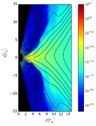
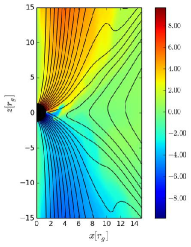
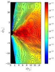
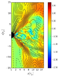
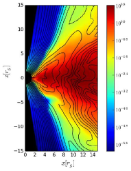
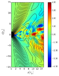
Figure 1.— Poloidal plane slices ($z$ vs. $x$) for snapshots in time of the dimensionless rest-mass density ($\rho r_{g}^{2}c/\dot{M}$, left panels) and dimensionless toroidal magnetic field scaled by radius ($(r/r_{\rm H})B_{\phi}r_{g}/\sqrt{c\dot{M}}$ with $B_{\phi}$ in Gaussian units, right panels) for the MAD_thick models (upper two panels), SANE_quadrupole-disk model (vertically-middle two panels), and SANE_dipole-jet model (lowest two panels). Magnetic field lines (from the $\phi$-integrated vector potential for clarity of the field behavior) are shown as black contour lines (negative contours are dashed, positive are solid, as originating from the initial values of the vector potential) with arbitrarily-sized uniform spacing to give $20$ contours within plotted domain. These are our simulation models with the default polar axis angle-based density cut-out (and no $b^{2}/\rho$-based removal procedure). The MAD_thick models have a relatively strong ordered poloidal and toroidal field in the jet, and the disk has an ordered magnetic field. The SANE_quadrupole-disk has no jet but does contain a toroidal magnetic field in a wind that has comparable strength in the disk. The SANE_dipole-jet model has a weak jet with an ordered toroidal and poloidal magnetic field, while the disk has a disordered toroidal field.

GRMHD simulations are typically based upon the ideal MHD equations of motion that assume no explicit viscosity, resistivity, or collisionless physics. Our ideal GRMHD simulations are based upon the ideal GRMHD code called HARM (Gammie et al., 2003), which has been used to perform several simulations to explore the role of BH spin (McKinney & Gammie, 2004; Gammie et al., 2004; McKinney, 2005; Tchekhovskoy et al., 2010; Tchekhovskoy & McKinney, 2012), magnetic field type (McKinney & Blandford, 2009; McKinney et al., 2012), large-scale jet propagation (McKinney, 2006), disk thickness (Shafee et al., 2008; Penna et al., 2010; Avara et al., 2015), how disks and jets pressure balance (McKinney & Narayan, 2007), relative tilt between the BH and disk (McKinney et al., 2013), and dynamically-important radiation (McKinney et al., 2014, 2015). Despite being ideal MHD solutions, they still provide the most state-of-the-art way of describing the fully three-dimensional global plasma behavior around a BH.

We use several previously published GRMHD models as input for the polarized radiative transfer calculations. The models used in this paper are labeled to designate the type of GRMHD simulation (MAD and SANE) followed by an identifier for the choices made for the radiative transfer scheme (-disk and -jet) for our primary models, for which we perform full fits (described in §2.7). In the following, we list the underlying GRMHD dynamical models used.

1. MAD_thick: A rapidly spinning $a/M=0.9375$ geometrically thick MAD model (McKinney et al., 2012) with a large-scale dipolar field with plentiful supply of magnetic flux. Dynamically produces a powerful jet with magnetic Rayleigh-Taylor instabilities. Includes rare magnetic field polarity inversions that drive transient jets (Broderick & McKinney, 2010).

2. SANE_quadrupole: A rapidly spinning $a/M=0.9375$ MRI disk model (McKinney & Blandford, 2009) with an initially large-scale quadrupolar magnetic field. Dynamically leads to no jet and contains an MRI-driven MHD-turbulent disk.

3. SANE_dipole: A rapidly spinning $a/M=0.92$ MRI disk model (McKinney & Blandford, 2009) with an initially dipolar magnetic field consisting of a single set of nested field loops following rest-mass density contours. Dynamically leads to a weak jet and MRI-driven MHD-turbulent disk.

Fig. 1 shows the set of three GRMHD simulations that form the basis of our various models. These models are all of relatively rapidly rotating BHs but span a range of types of magnetic fields in the disk (ordered and disordered) and jet types (powerful, weak, and no jet). Jet radiation could be an important contribution to observed emission even for Sgr A^∗ and might help explain the synchrotron self-absorption emission at low frequencies (Yuan et al., 2002; Mościbrodzka & Falcke, 2013). We only show the poloidal ($z$ vs. $x$) plane. All simulations have a toroidal direction with a turbulent toroidally-dominated disk at large radii and a more mixed laminar-turbulent (with equal toroidal and poloidal field strengths) disk at smaller radii near the photon orbit. The jet present in MAD_thick and SANE_dipole consists of a helical field with comparable poloidal and toroidal magnetic field strengths near the horizon (i.e., the light cylinder, or Alfven surface, where the toroidal field strength must become comparable to the poloidal field strength, is near the horizon for these high spin models). The SANE_quadrupole model has no BZ-driven jet or persistent low-density funnel region, but there is still a well-defined toroidally-dominated wind.

As discussed in detail in McKinney et al. (2012), the MAD_thick model very well-resolves the MRI and turbulent modes, the SANE_quadrupole model well-resolves the MRI and turbulent modes, and the SANE_dipole model marginally resolves the MRI and turbulent modes. A quasi steady-state inflow equilibrium is reached out to $r\sim 100r_{g}$ (gravitational radii) over a run-time of $30,000r_{g}/c$ ($180$ hours for Sgr A^∗) for the MAD_thick model, $r\sim 20r_{g}$ for the SANE_quadrupole model, and $r\sim 12r_{g}$ for the SANE_dipole model with both SANE models having run-time of $\sim 5,000r_{g}/c$ ($30$ hours for Sgr A^∗). Fig. 1 uses the snapshot at time $t=20612r_{g}/c$ for the MAD_thick model, $t=4280r_{g}/c$ for the SANE_quadrupole model, and $t=3200r_{g}/c$ for the SANE_dipole model.

2.2. Electron temperature prescription

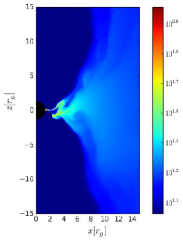
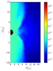
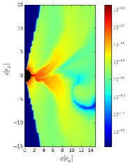
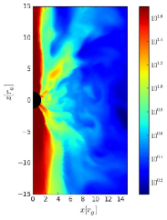
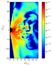
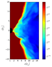
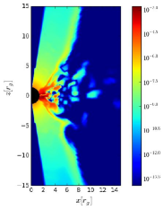
Figure 2.— Shows snapshot of electron temperature as $\log_{10}(\theta_{e})$ where $\theta_{e}=k_{\rm B}T_{\rm e}/(m_{\rm e}c^{2})$ (left panels) and arbitrarily scaled 230GHz synchrotron emissivity per unit mass accretion rate $\log_{10}(j_{\nu}/\dot{M})$ (right panels) for the MAD_thick-disk model (upper two panels), MAD_thick-jet model (next vertically-middle panels), SANE_quadrupole-disk model (next lower two panels), and SANE_dipole-jet model (next lowest two panels). These are our default models we consider for parameter fitting.

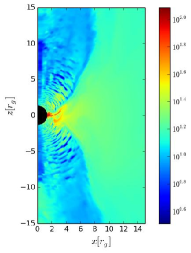
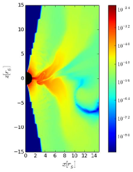
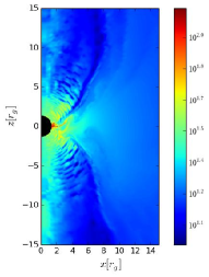
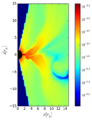
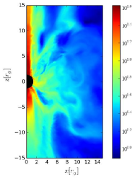
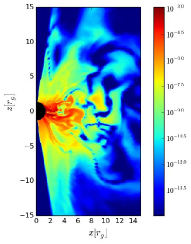
Figure 3.— Same as Fig. 2, but here using the alternative value of $\sigma_{T_{\rm e}}=40$ for the MAD_thick-disk model (upper two panels), MAD_thick-jet model (vertically-middle two panels), and SANE_quadrupole-disk model (lower two panels). Later discussions do not focus on how these parameters affect the SANE_dipole-jet model, so such variations in prescriptions are not shown for that model. As compared to Fig. 2, the higher $\sigma_{T_{\rm e}}=40$ pushes higher electron temperatures into the region with higher $b^{/}2\rho$, so that for the MAD_thick model higher electron temperatures are achieved in the funnel where $b^{2}/\rho\sim 50$. The higher $\sigma_{T_{\rm e}}$ leads to lower temperatures for much of the SANE_quadrupole-disk model, because polar material has only up to $b^{2}/\rho\sim 2$ and has no BZ-driven jet. Hence, $\sigma_{T_{\rm e}}=40$ allows us to focus higher isothermal temperatures in the BZ-driven funnel jet polar region if it exists in a model.

A major uncertainty in what leads to emission of Sgr A^∗ is the electron physics in weakly collisional plasmas. Often ad hoc prescriptions are adopted for electron temperatures. A “first-principle” approach as in pair plasma pulsar wind studies (Philippov et al., 2015) is computationally unfeasible at present, but some progress has been made.

We use the procedure described in Shcherbakov et al. (2012a) to modify the simulation proton and electron temperature based upon an evolution of the temperatures within the disk based upon the collisionless physics described by Sharma et al. (2007). This involves extending the simulation data from some radius ($r\sim 50r_{g}$ for MAD and $r\sim 30r_{g}$ for SANE) with a power-law extension out to the Bondi radius in Sgr A^∗. We use a density power-law of $\rho\propto r^{-0.85}$ and magnetic field strength scaling of $|b|\propto r^{-1}$, which are consistent with GRMHD simulations and the densities implied by Chandra X-ray observations (Shcherbakov et al., 2012a). This outer material primarily affects circular polarization and Faraday rotation measures as the polarized radiation passes through a significant column of toroidal field in the disk or corona.

The electron and proton temperatures are determined at all radii by a combination of the GRMHD simulations and an evolution equation for temperature. The temperature is evolved radially inwards from an initial temperature of $T_{\rm e}=T_{\rm p}=1.5\times 10^{7}$K at $r=3\times 10^{5}r_{g}$ implied by Chandra X-ray emission, while the density derives from the power-law extension mentioned above until small radii when the $\theta$- and $\phi$- averaged GRMHD simulation data is used. The evolution of $T_{\rm e}$ and $T_{\rm p}$ is controlled by proton-electron collisions (which dominate for $r\gtrsim 10^{4}r_{g}$), electrons being either non-relativistic or relativistic (matters for $r\lesssim 10r_{g}$ in the disk), and the electron to proton heating ratio $f_{\rm e}/f_{\rm p}=C_{\rm heat}\sqrt{T_{\rm e}/T_{\rm p}}$ for electron temperature $T_{\rm e}$ and proton temperature $T_{\rm p}$. This gives a result for the equatorial $T_{\rm e}$ and $T_{\rm p}$ vs. radius that uses both the GRMHD simulation data and radial extension model. As in our prior work, then, the original simulation’s temperature is modified by a mapping (at any $\theta$ or $\phi$) from the simulation value of the internal energy per unit rest-mass ($u/\rho$) to the evolution equation’s result for $T_{\rm e}$ and $T_{\rm p}$ (for more details see Shcherbakov et al. 2012a). This introduces another free model parameter $C_{\rm heat}$ that is nominally of order $C_{\rm heat}\sim 0.3$ (Sharma et al., 2007), but it may be quite small in the disk (Ressler et al., 2015). We identify this modified electron temperature computed for all points in space and time as $T_{\rm e,gas}$.

Most recently, the combined efforts of following electrons (Ressler et al., 2015) and protons (Foucart et al., 2015) suggest the proton temperature $T_{\rm p}$ is more isothermal than expected from ideal MHD for regions like the funnel-wall jet, where the electron temperature $T_{\rm e}$ rises up to $T_{\rm p}/2$ due to a high electron heating rate at low plasma $\beta=p_{\rm g}/p_{\rm b}$ (gas pressure $p_{\rm g}$ and magnetic pressure $p_{\rm b}$). The funnel-wall jet is defined by the boundary between the BZ-driven jet and the coronal wind where the magnetic field, density, and pressure change dramatically. This temperature prescription leads to a fairly isothermal electron temperature within the funnel-wall jet region, and this helps to produce the observed flat radio spectra (Mościbrodzka et al., 2014, 2015).

In order to mimic the isothermal approximation for the funnel-wall jet, we prescribe the electron temperature as a smooth transition from $T_{\rm e,gas}$ to a chosen value in the funnel-wall jet of $T_{\rm e,jet}$, using

$$T_{\rm e}=T_{\rm e,gas}e^{-b^{2}/\rho\sigma_{T_{\rm e}}}+T_{\rm e,jet}(1-e^{-b^{2}/\rho\sigma_{T_{\rm e}}}),$$ (1)

where $b^{2}/2$ is the magnetic energy density in Heaviside-Lorentz units and $\rho$ is the rest-mass density. This mimics what would be the combined results of Ressler et al. (2015) and Foucart et al. (2015) and is similar to what others have done when wanting to mimic the effects of emitting non-thermal particles in a jet (Mościbrodzka et al., 2014, 2015). The reference magnetization is given by $\sigma_{T_{\rm e}}$ that defines the jet funnel-wall boundary, where $\sigma_{T_{\rm e}}=1$ for MAD_thick-disk, SANE_quadrupole-disk, and SANE_dipole-jet models while $\sigma_{T_{\rm e}}=4$ for the MAD_thick-jet model. The funnel-wall jet electron temperature $T_{\rm e,jet}$ (per unit $m_{\rm e}c^{2}/k_{\rm B}$, hereafter we drop the $m_{\rm e}c^{2}/k_{\rm B}$ factor) is $T_{\rm e,jet}=10$ for model MAD_thick-disk, $T_{\rm e,jet}=35$ for model MAD_thick-jet, $T_{\rm e,jet}=50$ for model SANE_quadrupole-disk, and $T_{\rm e,jet}=100$ for model SANE_dipole-jet. For models (except SANE_dipole-jet), we also consider the alternative value of $T_{\rm e,jet}=100$.

The electron temperature prescription was chosen such that emission from the jet material was suppressed in the MAD_thick-disk model, whereas somewhat more jet emission was allowed in MAD_thick-jet. Parameters for the electron temperature prescription were chosen to represent a jet-dominated emission model for SANE_dipole-jet that contains a BZ-driven jet, and the electron temperatures were chosen to be disk-dominated for SANE_quadrupole-disk that contains no BZ-driven jet.

We use a smooth interpolation to prescribe electron temperatures and BZ-jet mass-loading, which avoids sharp features that can suddenly appear and disappear due to using hard cuts on a specific single value of a physical quantity, like plasma $\beta$ or the unboundedness of the fluid (Mościbrodzka & Falcke, 2013; Chan et al., 2015a). In future work, we will consider more advanced evolution equations for the electron temperatures (Ressler et al., 2015) and proton temperatures (Foucart et al., 2015).

2.3. Jet mass-loading prescription

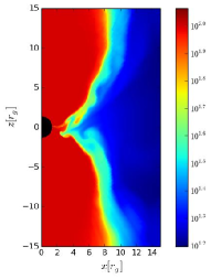
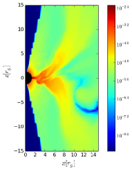
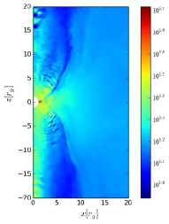
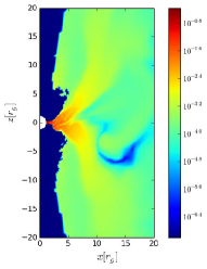
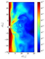
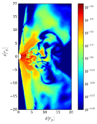
Figure 4.— Same as Fig. 2, but for the MAD_thick-jet model with $T_{\rm e,jet}=100$ (upper two panels), MAD_thick-jet model with $\sigma_{T_{\rm e}}=40$ and $\sigma_{\rho}=10$ (vertically-middle two panels), and SANE_quadrupole-disk model with $T_{\rm e,jet}=100$ (lower two panels). These panels show how the wind or jet emission is enhanced in different ways. Lighting up only self-consistent material that obeys mass conservation (middle two panels) leads to less BZ-jet funnel emission as compared to the otherwise similar model shown in Fig. 3. This way we can identify the difference between funnel-wall jet emission and BZ-driven funnel jet emission.

We control the rest-mass density in the BZ-jet funnel region where, nominally, matter is injected to keep the numerical scheme stable as necessary for any GRMHD code that models BZ jets (Gammie et al., 2003). The simulations we consider inject mass once $b^{2}/\rho>50$ (our MAD models) or $b^{2}/\rho>200$ (our SANE models), but this leads to much more mass accumulating near the stagnation radius (where the flow either moves in due to gravity or out due to the jet) (Globus & Levinson, 2013), leading to $b^{2}/\rho\gtrsim 10$ there. As long as the relativistic jet has not had much radial range to accelerate significantly, large values of $b^{2}/\rho$ do nothing to modify the GRMHD solution except to rescale the funnel density. So, the density could be chosen to be much higher (up to $b^{2}/\rho\sim 5$) or much lower without actually affecting the dynamics because the jet Lorentz factor never goes beyond $\gamma\sim 5$ (only occurring at large radii $r\sim 10^{3}r_{g}$, beyond the range of interest for this paper focused on horizon-scale structures).

By default, we control the density by only applying a polar axis cut-out, which removes material very near the polar axis that is numerically inaccurate and causes the densities to be momentarily artificially high. A similar approach is taken by others (Chan et al., 2015b). For MAD models, we remove material within $0.025$ radians, while for our SANE models we remove material within $0.01$ radians. This polar axis cut still leads to material being present near the horizon in the polar region that would represent some mass-loading of the jet. For the MAD model, this leads to a density in the funnel comparable to the density in the disk, and so the default MAD model can have (depending upon $T_{\rm e,jet}$) competing emission from the disk or jet. For the dipole model, the numerical floor-injected density in the funnel is much lower than in the MAD case, so only a very high temperature would (at some higher frequency) cause the funnel jet light up.

We also consider an alternative density removal procedure (still including the polar angle cut-out), where we remove the polar material using

$$\rho=\rho_{\rm gas}e^{-b^{2}/\rho\sigma_{\rho}}+\rho_{\rm jet}(1-e^{-b^{2}/\rho\sigma_{\rho}}),$$ (2)

with $\sigma_{\rho}=10$ and $\rho_{\rm jet}=0$, which for all models does a good job at removing material that is numerically injected near the BH. Here $\rho_{\rm gas}$ is the original simulation rest-mass density that includes the floor injection material. After removing of the density using $\sigma_{\rho}=10$ and $\rho_{\rm jet}=0$, only self-consistent material that obeys conservation of mass is left. The default polar axis angle-based density removal procedure keeps funnel jet material that is dependent upon uncertain mass-loading physics. For the SANE_quadrupole-disk model, there is never any region with $b^{2}/\rho\gtrsim 2$, so only the polar angle cut matters. In future work, we will consider simulations that directly track the injected mass.

Fig. 2 shows the coordinate x-z plane for our default models (i.e., models with default choices for electron temperature and mass-loading prescriptions). The figures show the electron temperature and the arbitrarily scaled 230GHz thermal synchrotron emissivity, which helps to identify the origin of emission seen in the final radiative transfer results. In some cases, like the SANE_quadrupole-disk model, low-level emissivity is truncated a bit by the density removal or polar cuts, but in other models the polar axis density cut-out has little effect on the emissivity.

Fig. 3 shows some alternative electron temperature prescriptions using a higher $\sigma_{T_{\rm e}}=40$. Fig. 4 show cases where $T_{\rm e,jet}=100$ or our alternative mass-loading choice. In the MAD_thick model, our default polar angle cut-off only cuts-out matter that was injected by the numerical floors but does a poor job of removing all injected material, because its primary purpose was to only remove material near the polar axis. Our alternative additional cut-off using $\sigma_{\rho}=10$ somewhat accurately removes the numerically-injected floor material (McKinney et al., 2012).

2.4. Polarized radiative transfer scheme

The data from GRMHD simulations presented in the previous section serve as input for a general relativistic polarized radiative transfer scheme (Shcherbakov, 2014; Shcherbakov & Huang, 2011), an extended version of ASTRORAY (Shcherbakov et al., 2012b). In its present stage, the code assumes a thermal, isotropic distribution function for the electrons, and it includes Faraday rotation and conversion. The code has been used to model polarized synchrotron emission and absorption of Sgr A^∗ in the past (Shcherbakov et al., 2012b; Shcherbakov & McKinney, 2013a).

The ASTRORAY code performs direct transfer of light through the entire GRMHD simulation’s dependence vs. space and time. The GRMHD data is sampled every $4r_{g}/c$ (MAD model, $1.4$ minutes for Sgr A^∗) or $2r_{g}/c$ (SANE models, $0.7$ minutes for Sgr A^∗). We do not use the so-called fast-light approximation, which assumes an infinite speed of light. The fast-light approximation has been found to be inaccurate on timescales less than $10r_{g}/c$ ($3.5$ minutes for Sgr A^∗) (Shcherbakov et al., 2012b) and can considerably change the character of the behavior in time (Dexter et al., 2010). The fast-light approximation may lead to stronger lensing features, which would otherwise be washed out, because nearby emitting regions would not as easily correlate their emission. This also means we do not have to choose between a time-averaged flow (to try to obtain a more realistic distribution of density and other plasma properties for each snapshot) vs. the average of snapshots (see discussion in Chan et al. 2015b). For our models, errors introduced by the fast-light approximation at $f\geq 230{\rm GHz}$ exceed $\Delta F/F\gtrsim 15\%$, although the effects are insignificant at lower frequencies. Instead, we compute snapshots (or time-averages of snapshots) in the observer’s reference frame using transfer through the full time-dependent simulation data.

As compared to prior similar work (Dexter et al., 2009; Mościbrodzka et al., 2009; Dexter et al., 2010; Mościbrodzka et al., 2014; Chan et al., 2015a, b), no other work has considered the role of polarization with GRMHD simulations except our own prior works (Shcherbakov et al., 2012b; Shcherbakov & McKinney, 2013a) and preliminary work by Dexter (2014). The MAD_thick-disk model is similar to models used in prior polarimetric work by us (Shcherbakov et al., 2012a; Shcherbakov & McKinney, 2013a). The SANE_quadrupole-disk model has not been used before in polarized radiative transfer studies. The SANE_dipole-jet model has been used in prior studies of both Sgr A^∗ (Dexter et al., 2010) and M87 (Dexter et al., 2012) without polarization, while the SANE_dipole-jet model has been applied to parsec-scale active galactic nuclei jets with polarization and Faraday rotation (Broderick & McKinney, 2010).

2.5. Scattering

For image plane quantities, we apply a simple circular Gaussian blurring to simulate the effects of scattering off inhomogeneities in the ionized interstellar medium. The width of the Gaussian is lowered by a factor of two to account for the possible (partial) mitigation technique presented in Fish et al. (2014).

However, no scattering kernel is applied to the visibility plane quantities (see §2.8), so our results should be compared with data that have been “deblurred” using the estimated scattering kernel extrapolated from longer wavelengths (see Fish et al., 2014).

2.6. Image Plane Quantities

We generate synthetic images for each Stokes parameter $\{I,Q,U,V\}$ for all models and as a function of time. $I$, representing intensity, is a non-negative quantity, while positive or negative $V$ corresponds to right and left circular polarization, respectively, following IAU/IEEE definition of the sign of circular polarization. The linear polarization intensity is given by $LP=\sqrt{|Q|^{2}+|U|^{2}}$, where linear polarization fraction is given as per unit intensity in percent. The linear polarization direction, or electric vector position angle (EVPA) is determined by the argument of the complex polarization field: ${\rm EVPA}={\rm arg}(Q+iU)/2$, corresponding to the angle of the electric polarization EAST of NORTH. Circular polarization fraction is given as $V$ per unit $I$ in percent. These additional diagnostics are used to assess further the viability of each model beyond the spectrum of image and time-averaged quantities.

2.7. Model Fitting

The free parameters in our radiative transfer model are:

• inclination: $i$

• heating ratio between electrons and protons: $C_{\rm heat}$

• Mass accretion rate normalization: $\dot{M}$

We determine the mass accretion rate, inclination ($i=0$ is face-on, while $i>0$ moves toward NORTH), and heating ratio by fitting the measured fluxes and image-integrated linear and circular polarization as in Shcherbakov et al. (2012b). Specifically, we fit (unpolarized) fluxes at 7 frequencies from $f=87{\rm GHz}$ to $f=857{\rm GHz}$, 3 linear polarizations at $f=\{87{\rm GHz},230{\rm GHz},349{\rm GHz}\}$, and 2 circular polarizations at $f=\{230{\rm GHz},349{\rm GHz}\}$ resulting in 9 degrees of freedom (3 free parameters).

We employ a steepest descent method to minimize $\chi^{2}$ as in Shcherbakov et al. (2012b) where $\chi_{I}^{2}=\sum_{i}(F_{\nu,i}-F^{\rm obs}_{\nu,i})^{2}/\Delta F^{2}_{\nu,i}$ with $F_{\nu,i}$ are the computed fluxes, $F^{\rm obs}_{\nu,i}$ are the observed fluxes (averaged as described and tabulated in Shcherbakov et al. (2012b) and $\Delta F_{\nu,i}$ are errors, see Shcherbakov et al. (2012b). We compute the analogous quantity $\chi^{2}_{P}$ for polarization using $LP@\{87{\rm GHz},230{\rm GHz},349{\rm GHz}\}=\{1.4\pm 0.5\%,7.4\pm 0.7\%,6.5\pm 0.6\%\}$ and $CP@\{230{\rm GHz},349{\rm GHz}\}=\{-1.2\pm 0.3\%,-1.5\pm 0.3\%\}$. The total residual of the fits is then $\chi^{2}=\chi^{2}_{I}+\chi^{2}_{P}$. In the table we quote $\chi^{2}$ and the resulting $\chi^{2}_{I}$ (even though the latter was not separately fitted for). Note, that this procedure does not optimize the fit for $230{\rm GHz}$ (the main focus of this work) in any way. We exclude from the fits any lower frequencies for which non-thermal particles could be required, with the goal of not biasing our models at $230{\rm GHz}$. EVPA is not included in the fits just like prior work using ASTRORAY Shcherbakov et al. (2012b); Shcherbakov & McKinney (2013a), because it is influenced by the uncertainties in the radial extension. These important aspects will be tackled in future work.

Similar to previous work there are nuisance model parameters, including $\sigma_{T_{\rm e}}$, $T_{\rm e,jet}$, $\sigma_{\rho}$, which we only vary as part of a specific model and do not minimize $\chi^{2}$ over. Some prior works directly include image size in the fitting procedure as additional observational data (Chan et al., 2015b), but we do not. In principle, we could tune our fitting procedure to primarily fit the 230GHz emission (the main focus of this work) instead of just by the error of each independent observation. This was useful for the SANE_dipole-jet model, for which we slightly adjusted the original fit parameters in order to get better agreement with linear polarization at 230GHz. We plan further development of fitting procedures.

2.8. VLBI Visibility Plane Quantities

After fixing the free parameters as determined from the fits to image-integrated flux, linear polarization, and circular polarization, we generate the corresponding Fourier transformed visibility data $\{\tilde{I},\tilde{Q},\tilde{U},\tilde{V}\}$. We focus on measurements of fractional linear and circular polarization in the visibility domain: $\breve{m}\equiv(\tilde{Q}+i\tilde{U})/\tilde{I}$ and $\breve{v}\equiv\tilde{V}/\tilde{I}$, respectively. Note that each of these quantities is complex. We also compute the visibility domain ${\rm EVPA}={\rm arg}((\tilde{Q}+i\tilde{U})/\tilde{I})/2$. The amplitudes and phases of these visibility domain ratios are immune to a wide range of station-based calibration errors and uncertainties and thus provide excellent VLBI observables (Roberts et al., 1994). Fractional polarization in the visibility domain is also insensitive to the ensemble-average “blurring” effect of scattering (Johnson et al., 2014), which increases the thermal noise in measurements but does not bias them. Because we do not include thermal noise in the current comparisons with observations, when applicable (e.g., for $|\tilde{I}|$), we show quantities that would be obtained after “deblurring” (Chan et al., 2015b). In practice, long baselines may show slight additional variations from “refractive substructure,” which will vary stochastically with a timescale of ${\sim}1~{}{\rm day}$ (Johnson & Gwinn, 2015).

3. Results

In this section, we present the results of our polarized radiative transfer calculations. We describe our findings for each GRMHD model, quantify the level of agreement with several observational constraints and point out remaining issues, and elaborate on the different trends seen between different models.

3.1. Results of Zero-Baseline Model Fitting

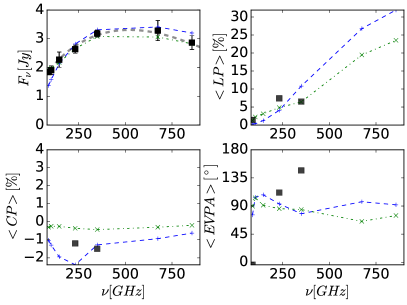
Figure 5.— Spectral energy distribution (SED, $F_{\nu}$ in Jy), fractional linear polarization $<\!\!\!LP\!\!\!>$, fractional circular polarization $<\!\!\!CP\!\!\!>$, and electric vector position angle $<\!\!\!EVPA\!\!\!>$ (all image-integrated) vs. frequency in GHz for model MAD_thick-disk (green dotted line and cross) and SANE_quadrupole-disk (blue dashed line and plus). Positive or negative $<\!\!\!CP\!\!\!>$ corresponds to right and left circular polarization, respectively. These model data are compared to the observed data (black squares) and a fit through observed data (grey dashed line). See Tab. 1 for results from fitting. More work is needed on our model that extends the simulation data to large radii in order to fit the frequency-dependence of CP and EVPA. The frequency dependence of image-integrated flux and linear polarization measurements are in good agreement with our models, while CP and EVPA are roughly the right magnitude (except for one observation of low EVPA, but we do not fit for EVPA).

Table 1List of models considered including parameters: $i$ inclination ($i=0$: face-on), $C_{\rm heat}$ (related to the electron-to-proton heating ratio for the disk), $\dot{M}$ rest-mass accretion rate, and $\chi^{2}/{\rm dof}$ (fitted to I,LP, and CP) and $\chi^{2}_{I}/{\rm dof}$ (fitted only to unpolarized I) (dof: degrees of freedom) quantifying the goodness of fit.

Model	$i$	$C_{\rm heat}$	$\dot{M}$ [$\frac{M_{\odot}}{{\rm yr}}$]	$\frac{\chi^{2}}{{\rm dof}}$	$\frac{\chi^{2}_{I}}{{\rm dof}}$
MAD_thick-disk	$99^{\circ}$	$0.025$	$5.5\times 10^{-9}$	$4$	$0.5$
MAD_thick-jet	$140^{\circ}$	$0.05$	$5.4\times 10^{-9}$	$5$	$8$
SANE_quadrupole-disk	$98^{\circ}$	$0.47$	$4.0\times 10^{-8}$	$7$	$7$
SANE_dipole-jet	$126^{\circ}$	$0.55$	$2.6\times 10^{-8}$	$13$	$12$

We first consider the frequency-dependent zero baseline observations as compared to our models. Fig. 5 shows our model fits using the default electron temperature and mass-loading prescriptions using the fitting procedure discussed in section 2.7 with an assumed BH mass of $M=4.3\times 10^{6}{\rm M_{\odot}}$. We time-averaged spectra over an interval $4000r_{g}/c-5600r_{g}/c$ for SANE_quadrupole-disk, $2500r_{g}/c-3300r_{g}/c$ for SANE_dipole-jet, and $20212r_{g}/c-22212r_{g}/c$ for our MAD models.

The fits to $I$, $LP$ percentage, and $CP$ percentage give an intensity vs. frequency with a relatively good fit for any model. Linear polarization adds an additional constraint on the inclination angle due to how different inclination angles lead to varying amounts of cancellation in polarized emission from different parts of the disk or jet. We do not fit EVPA, which is not fit well vs. frequency, although their values are roughly correct. We do not focus on fitting EVPA because it is controlled by the flow at larger radii than the simulations reach a steady-state out to. In principle, fitting to intensity alone will produce a different fit than our fitting to $I$, $LP$, and $CP$, which may affect prior intensity-only fits, but we did not consider intensity-only fits in this paper. For SANE_dipole-jet, we slightly adjusted the original fit to obtain better agreement for the linear polarization fraction at $230$GHz (The original overall lowest $\chi^{2}/{\rm dof}$ was for $i=124^{\circ}$, $C_{\rm heat}=0.47$ and $\dot{M}=3.6\times 10^{-8}{\rm M_{\odot}}/{\rm yr}$, extremely similar to our slightly tuned fit.).

The fits prefer different inclination angles for the jet and disk cases. For the disk cases, the inclination must be close to edge-on (${\approx}10^{\circ}$ above edge-on), whereas for the jet models it must be much higher (${\approx}45^{\circ}$ below edge-on).

The MAD_thick-disk model did not need an isothermal jet or non-thermal particles to account for the low frequency flux seen in Fig. 5. The MAD model constrains a hot funnel-wall visible as high emissivity in Figs. (2,3,4) for any electron temperature prescription. At much larger radii, the prescription for the electron temperature still ensures that enough material is close to isothermal, which is sufficient to fit the low-frequency synchrotron self-absorption part of the spectrum.

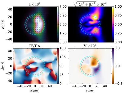
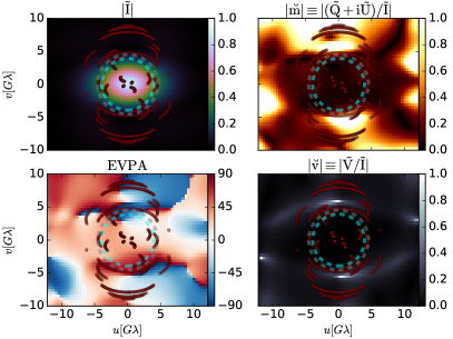
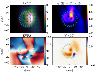
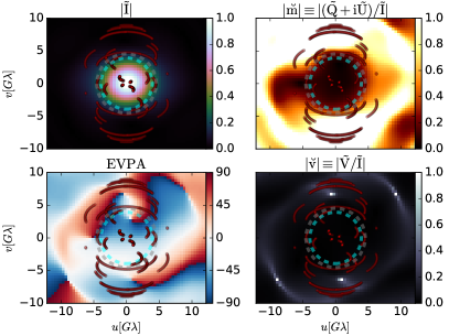
Figure 6.— All Stokes parameters and several derived quantities in the image plane (intensity $I$ in Jy/pixel with overlaid polarization ticks that scale in length with $LP=\sqrt{|Q|^{2}+|U|^{2}}$ and are oriented by the EVPA, linear polarization intensity $\sqrt{|Q^{2}|+|U|^{2}}$ in Jy/pixel, EVPA showing angle of electric field polarization, and $|V|$ showing magnitude of circular polarization) and visibility plane (Fourier intensity $|\tilde{I}|$, fractional linear polarization $|\breve{m}|$, EVPA showing polarization angle, and $|\breve{v}|$ showing fractional circular polarization) at $f=230{\rm GHz}$ for model MAD_thick-disk (upper panel) and MAD_thick-jet (lower panel) from snapshots in time. All such plots have $151\times 151$ pixels for quantities given in per pixel. Dashed circles indicate the expected shadow size for a back-lit BH that has no spin (cyan, $\approx 10.4r_{g}$) or has maximal spin (grey, $\approx 9r_{g}$, roughly averaged over viewing plane angle and inclination with respect to the BH spin axis, see Takahashi 2004). Tracks are shown in the $uv$ plane that will be probed by the EHT in 2017 (see Johnson et al. 2015a for site details). These figures give a general impression of the relationship between image and visibility domain. The visibility plots are further useful to judge the importance of baseline coverage and source orientation.

3.2. Image and Visibility Plane

For the default models that we fit zero baseline observations to in the previous section, we next consider what the full image and visibility planes reveal. Figs. 6 and 7 show all Stokes parameters for our default set of four models at the same time show for Figs. (1,2,3,4) in section 2.1. No time-averaging is performed.

In these and similar plots, the image plane has the BH spin axis pointing along the vertical (NORTH) direction, where the left-direction is WEST and right-direction is EAST (as if seeing projected image on surface of Earth and the EHT), while sometimes the opposite choice is made for EAST-WEST as if one is viewing the source. The image plane linear ($Q$ and $U$) and circular polarization ($V$) are not shown as fractional values, so that the primary polarized emitting regions can be identified. Visibility plane linear polarization ($\breve{m}$) and circular polarization ($\breve{v}$) are shown as fractions, consistent with what the EHT can most robustly measure.

Across all these models, polarization persists to longer baselines (smaller scale structure) than total intensity. In temporal evolutions of such plots, stronger variability is seen generally on longer baselines as expected. These findings suggest that the emission fine-scale structure is best constrained by high resolution (in time and space) polarization studies, and they highlight the growing importance of polarization as the EHT expands to longer baselines (Fish et al., 2009, 2013; Ricarte & Dexter, 2015).

In all our models, the image plane polarization is highest outside from where the image plane intensity is highest. Regions with highest total intensity have somewhat lower (but still significant) polarization. Therefore, the visibility plane intensity will show the different scale of intensity and polarization as a high visibility fractional polarization due to regions with relatively lower intensity. Hence, accurate high fractional polarization measurements can only be achieved with sensitive measurements to detect and characterize points with little correlated total-intensity flux $\tilde{I}$ (Johnson et al., 2015b).

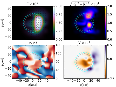
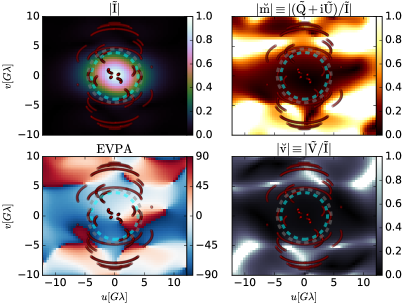
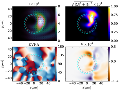
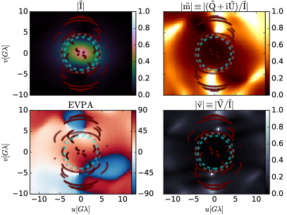
Figure 7.— Same as Fig. 6, but for models SANE_quadrupole-disk (upper panels) and SANE_dipole-jet (lower panels). The BH shadow in both intensity and polarization are considerably different than the MAD models, suggesting detectability of the BH shadow feature may have to account for such model variations.

3.3. Observational Constraint on Magnetic Field Structure

In Johnson et al. (2015b), it is shown how EHT data constrain the degree of order in the magnetic field in the emission region by comparing the relative amplitudes of two dimensionless quantities: the visibility plane fractional polarization with the visibility domain normalized intensity. The price one has to pay by using $\breve{m}$ is that the interpretation is not as straightforward as with the image plane fractional polarization. The quantity $\breve{m}\equiv(\tilde{Q}+i\tilde{U})/\tilde{I}$ is a measure of linear polarization in the visibility (Fourier) domain, but its inverse Fourier transform is not the fractional linear polarization in the image domain $m_{LP}\equiv(Q+iU)/I$. However, direct comparisons can still be made between observations and models (Johnson et al., 2015b).

Following Johnson et al. (2015b), Fig. 8 shows $|\breve{m}|$ as a function of normalized total intensity $|\tilde{I}/\tilde{I}_{0}|$ for all of our default models and the asymptotic cases described in Johnson et al. (2015b), where $\tilde{I}_{0}$ is the correlated flux density on the zero-baseline. For uniform polarization across the image one expects $|\breve{m}(|\tilde{I}/\tilde{I}_{0}|)|={\rm const}{.}$, whereas for maximally disordered fields $|\breve{m}(|\tilde{I}/\tilde{I}_{0}|)|\propto\tilde{I}_{0}/\tilde{I}$ on average. Our simulations confirm that EHT measurements of $\breve{m}$ indicate the magnetic field’s degree of order vs. disorder, preferring both MAD models over both SANE models.

Unlike other image and polarization characteristics, these conclusions are relatively insensitive to the viewing inclination. Fig. 9 shows the average of $|\breve{m}(|\tilde{I}/\tilde{I}_{0}|)|$ for a fixed fiducial model (MAD_disk) at varying inclination. The results are similar over a range of $40^{\circ}$, showing that this metric of field order is fairly robust. Figure 10 shows the varying models but for $|\breve{v}|$, the visibility plane circular polarization fraction (note that EHT data for $\breve{v}$ are not yet available). Here we see that the MAD models are not clustered together, and instead the jet models tend to have high $|\breve{v}|$ and the disk models tend to have lower $|\breve{v}|$. More extensive comparisons are necessary to conclude whether $|\breve{v}|$ can help distinguish disk vs. jet models in general.

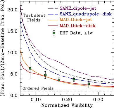
Figure 8.— Fractional linear polarization $|\breve{m}|$ (as measured in the visibility plane) per unit zero baseline value vs. the normalized visibility $|\tilde{I}/\tilde{I}_{0}|$ for all models. Observational data from the EHT are shown as green squares. Asymptotic results for perfectly ordered fields are shown as a horizontal dashed black line and for completely turbulent fields as a curved dashed black line. SANE models are shown as colored dashed lines and MAD models as colored solid lines. Our MAD models are preferred over our SANE models. SANE_quadrupole-disk with a large-scale quadrupolar field in the disk is only marginally inconsistent with observations.

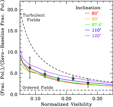
Figure 9.— Same as Fig. 8, but showing five different viewing inclinations of the MAD_thick-disk model while holding all other parameters fixed. The middle value ($i=97.4^{\circ}$) is the fiducial case used throughout the paper. Unlike other observables, such as the total flux and image size, $|\breve{m}|$ vs. $|\tilde{I}/\tilde{I}_{0}|$ is relatively insensitive to the changing inclination and robustly quantifies the order of the magnetic field throughout the emission region.

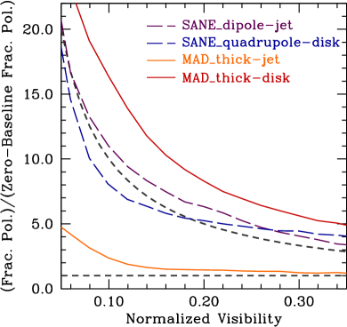
Figure 10.— Similar to Fig. 8, but showing fractional circular polarization $|\breve{v}|$ per unit zero baseline value (as measured in the visibility plane) vs. normalized visibility $|\tilde{I}/\tilde{I}_{0}|$ for all models. No EHT data yet exists, but apparently jet models tend to have higher $|\breve{v}|$ than disk models, so $\breve{v}$ might help differentiate between disk and jet models and provide a unique constraint compared to linear polarization via $\breve{m}$.

3.4. Variability

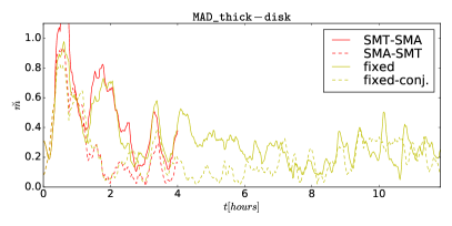
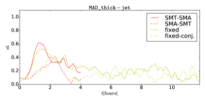
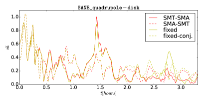
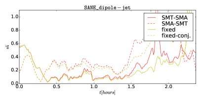
Figure 11.— Value of $|\breve{m}|\equiv|\tilde{Q}+i\tilde{U}|/|\tilde{I}|$ vs. time along the SMA-SMT baseline (red/dark) and at fixed (stationary) baselines (yellow/light) and as a function of time $t$ for models MAD_thick-disk (upper left panel), MAD_thick-jet (upper right panel), SANE_quadrupole-disk (lower left panel), and SANE_dipole-jet (lower right panel). All data sets are variable, but only the MAD models have QPOs (less visible at the orientation chosen for the MAD_thick-jet model) (McKinney et al., 2012; Shcherbakov & McKinney, 2013b). Note that differences between conjugate baselines arise from polarization alone and vary greatly between models. Both SANE and MAD models give high enough $\breve{m}$ amplitude and asymmetry for well-chosen baseline orientations, but the MAD models are consistent for a broader set of baseline orientations.

In this section, we consider how non-zero baselines at $230$GHz with linear polarization provide additional constraints on the models beyond zero baseline frequency-dependent observations. The simplest EHT observation is to only consider a single baseline consisting of a specific antenna pair at various points in time. Each physical baseline has two directions but provides a single measurement in intensity and fractional circular polarization ($\tilde{I}(u,v)=\tilde{I}^{\ast}(-u,-v)$ and $\breve{v}(u,v)=\breve{v}^{\ast}(-u,-v)$) because their corresponding images are real. However, the baseline provides two independent linear polarization measurements $\breve{m}(\pm u,\pm v)$ because the linear polarization image $Q+iU$ is complex.

Fig. 11 shows light curves for $\breve{m}$, which take into account the time dependence of the emissivity from the GRMHD simulation and the evolution of the flow during radiative transfer (no fast-light approximation). The MAD models show data from $20212r_{g}/c-22212r_{g}/c$, SANE_quadrupole-disk shows $4000r_{g}/c-4560r_{g}/c$, and SANE_dipole-jet $2800r_{g}/c-3200r_{g}/c$. We consider both fixed and changing baseline orientations (due to the rotation of the Earth) computed for an EHT campaign, where the fixed case just chooses the starting point from the case with changing baseline positions. As a reference point, the EHT data show up to $|\breve{m}|\sim 70\%$ on one baseline point $\{u,v\}$ while at the same time showing $|\breve{m}|\sim 30\%$ for the conjugate baseline point $\{-u,-v\}$. For angles EAST of NORTH, model MAD_thick-disk used $0^{\circ}$, MAD_thick-jet used $+45^{\circ}$, SANE_quadrupole-disk used $-45^{\circ}$, and SANE_dipole-jet used $-23^{\circ}$ for the relative baseline orientation.

All models are highly dynamic with a tendency for larger variation at larger baseline lengths. Both the amplitude of variations in $|\breve{m}|$ and the differences between opposite baselines are more consistent with observations for the MAD models than for the SANE models. The MRI type disk in model SANE_quadrupole yields less variability and smaller $\breve{m}$ even on these baselines that were optimally chosen to give agreement with EHT observations, but all models can potentially at some moments in time reproduce the amplitude and asymmetry of $\breve{m}$ seen in EHT data. As shown in Shcherbakov & McKinney (2013a), the MAD models have quasi-periodic oscillations (QPOs) clearly apparent in linear polarization, which may also help distinguish between MAD and SANE models. Longer and more frequent EHT observations could provide further insight by using more rigorous statistical comparisons.

Our synthetic data show dynamical activity of the source size and correlated flux. A local minimum in the correlated flux density observed on day 80 in the 2013 EHT campaign could be due to such natural variability in the underlying accretion flow. The level of variability in all models may be sufficient to produce dips in the correlated flux as observed on some days. Comparing or finding agreement in such temporal features is an interesting and important avenue which we will pursue in more detail in the future.

The absolute position angle orientation of the simulated images is a priori unknown. As shown in the prior figures, $\breve{m}$ is more clearly anisotropic in the visibility plane than $\tilde{I}$ (that is fairly Gaussian), so polarization on sufficiently long baselines is more sensitive to the absolute position angle orientation. The extra information from polarization can help constrain models that have to match both the magnitude and asymmetry in $\breve{m}$ vs. time for both conjugate points in a baseline.

Fig. 12 shows light curves from the MAD_thick-disk model for 8 different image orientations in the uv-plane at an angle EAST of NORTH by $\in[-90,-67.5,-45,-22.5,22.5,45,67.5,90]$. Only if the SMT-SMA baseline is oriented between $\pm 45^{\circ}$ in the visibility plane would the magnitude and asymmetry from the simulations match the EHT data. Orientations too close to the $u$ (WEST-EAST) axis lead to no large values of $\breve{m}$ and weak asymmetry. For other models, like SANE_dipole-jet, $\breve{m}$ is high only in small patches in the uv plane on these EHT baseline lengths. This comparison alone does not allow us to exclude the SANE_dipole-jet model, but more EHT baselines (i.e., beyond EHT 2013) might enable such exclusions.

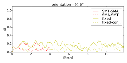
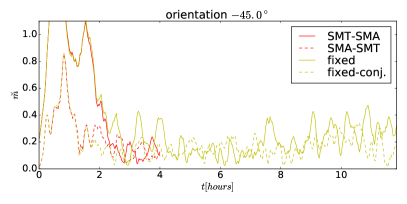
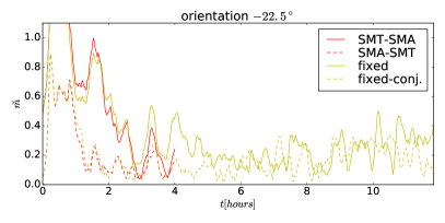
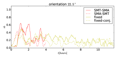
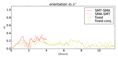
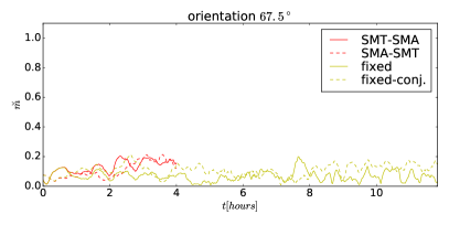
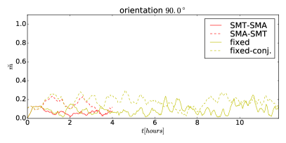
Figure 12.— Same as Fig.11 for MAD_thick-disk model but for 8 different orientations EAST of NORTH given by $\in[-90,-67.5,-45,-22.5,22.5,45,67.5,90]$ (from left to right, top to bottom). For a given baseline orientation, the fixed baseline case does not move the baseline position vs. time. For the SMT-SMA and SMA-SMT baseline positions, the baselines move with time consistent with the EHT. The agreement with EHT data for $\breve{m}$ vs. time is not possible with any baseline orientation. The EHT data reaches up to $\breve{m}\sim 70\%$ and the SMT-SMA baselines show significant asymmetry in the magnitude (down to $\breve{m}\sim 30\%$ for the other side of the baseline). Only baseline orientations that are $-45^{\circ}$ to $+45^{\circ}$ show sufficient amplitude and asymmetry, allowing one to constrain how the position angle of the model data relative to the EHT baselines. Such a constraint is not possible with intensity only (assuming an anisotropic scattering kernel does not help resolve the position angle).

3.5. Intensity and Polarization vs. Baseline Length

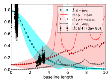
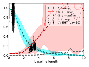
Figure 13.— Model MAD_thick-disk (left panel) and MAD_thick-jet (right panel) showing $|\tilde{I}|$, $|\breve{m}|$, and $|\breve{v}|$ as a function of baseline length. Shaded regions span the variation along all baseline orientations. Both models produce high polarization on longer baselines. Sharp $\breve{m}$ and $\breve{v}$ peaks are associated with baseline lengths with where $\tilde{I}$ falls close to zero.

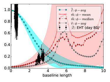
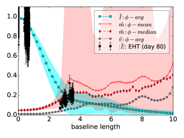
Figure 14.— Same as Fig. 13 for models SANE_quadrupole-disk (left panel) and SANE_dipole-jet (right panel). The SANE_quadrupole-disk produces large scale polarization features comparable to MAD models. The SANE_dipole-jet model shows a partial shadow feature with a broad crescent, which leads to a larger image size and more consistency with the observations on shorter baseline lengths.

Figs. 13 and  14 show the total intensity and polarization fractions as a function of baseline length. The polarization features are significantly more distinguishing than the unpolarized emission.

The MAD models MAD_thick-jet and MAD_thick-disk readily produce the observed polarization, despite emission from the jet region being suppressed in the MAD_thick-disk model. All models have fractional linear polarization in the image domain that reach comparable levels to recent EHT measurements.

It is apparent from the images that the total intensity features can be similar for the MAD and SANE_quadrupole-disk models, but the polarization fields are clearly distinct. This is promising for the prospect of disentangling different magnetic field structures and constraining models in a way not possible with only intensity.

3.6. Dependence on Electron Temperature and Mass-Loading Prescriptions

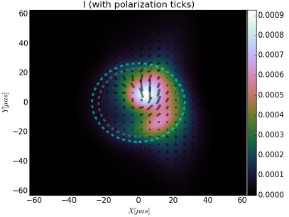
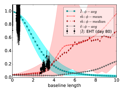
Figure 15.— Image with overlaid polarization ticks and visibility domain quantities vs. baseline length for a model similar to MAD_thick-jet, but with $\sigma_{T_{\rm e}}=40$ corresponding to enhanced jet emission. Dashed circles indicate the expected shadow size for a non-spinning (cyan) and maximally spinning (grey) BH. For this data set the density scale and hence the accretion rate have been adjusted to be consistent with the observed flux density at 230GHz. The emission size is smaller and $|\breve{m}|$ is generally lower than for the fiducial MAD_thick-jet. The BH shadow feature is more filled-in due to the enhanced jet emission. A more exhaustive parameter search might find cases where this jet-enhanced emission model produces a less compact emission, as is required by EHT measurements of $|\tilde{I}|$.

The specific electron temperature prescription is uncertain, so we consider variations away from our default model for $\sigma_{T_{\rm e}}$. Fig. 15 shows the same plots as before for the MAD_thick-jet model, but for $\sigma_{T_{\rm e}}=40$. In this case, the BZ-funnel jet (not just the funnel-wall jet) has its emission boosted. This occurs because the BZ funnel has $b^{2}/\rho\sim 30$–$50$ near the BH, and so changing $\sigma_{T_{\rm e}}$ from $1$ to $40$ leads to much more of the material in the funnel having a higher temperature given by $T_{\rm e,jet}=35$.

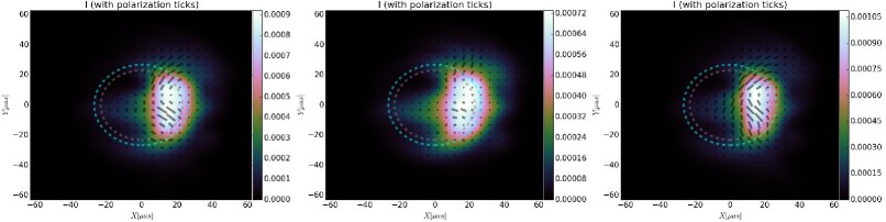
Figure 16.— Progression of image plane intensity and overlaid polarization ticks for models like SANE_quadrupole-disk model (left panel) with modified $\sigma_{T_{\rm e}}=40$ (middle panel) consistent with Figs. 3, and modified $T_{\rm e.jet}=100$ (right panel) consistent with Figs. 4. In both modified cases the density scale and thus accretion rates was adjusted by $\sim 30\%$ to roughly fit the observed zero baseline flux. Differences in polarization ticks are dramatic, but changes are minor in intensity despite the electron prescription forcing more radiation to be emitted from the coronal regions. This shows how polarization could be more sensitive to the electron temperature prescription than intensity.

Fig. 16 shows the SANE_quadrupole-disk model with different electron temperature prescriptions, including our default choice, $\sigma_{T_{\rm e}}=40$, and $T_{\rm e,jet}=100$. These change the image size slightly, but the $\sigma_{T_{\rm e}}=40$ has a quite different polarization pattern. This suggests that polarization might be more sensitive to changes in the electron heating physics or whether a BZ-driven funnel jet contains hot electrons.

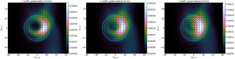
Figure 17.— Progression of image plane intensity plots with overlaid polarization ticks for models like MAD_thick-jet, but with $\sigma_{\rho}=10$ (left panel), $\sigma_{\rho}=35$ (middle panel), and $\sigma_{\rho}=100$ (right panel, consistent with our default model shown in lower panels of Fig. 6) with $\rho_{\rm jet}=0$ to force the material with $b^{2}/\rho>\sigma_{\rho}$ to have a lowered density value. The left panel with $\sigma_{\rho}=10$ is consistent with removing all numerically-injected floor material, leaving only self-consistently evolved material that follows from mass conservation. This removes a significant amount of emission from the BZ-driven funnel jet, creating a hole in the emission that mimics a BH shadow feature. The middle and right panels show the progression toward our default MAD_thick-jet model that includes the BZ-driven funnel jet material (whose emissivity is also controlled by the electron temperature prescription). These panels show how BZ-driven funnel and funnel-wall jets might be distinguishable.

The mass-loading mechanism for BZ-driven funnel jets remains uncertain, so we vary the mass-loading via changes in $\sigma_{\rho}$ and consider how it changes the intensity and polarization in the image plane. Fig. 17 shows how emission from the BZ-driven funnel jet normally fills-in the BH shadow region in the MAD_thick-jet model as was shown in Fig. 6. The BZ-jet funnel material violates mass conservation, because matter is injected (indirectly motivated by photon annihilation or pair production cascades) in order to maintain code stability. By removing the funnel density material, only self-consistently evolved matter that obeys mass conservation is left that exists in the funnel-wall jet, corona, and disk. The self-consistent material has no funnel emission, so the image plane recovers a BH shadow feature that was previously obscured by BZ-driven funnel jet emission. So, the image plane (and corresponding Fourier transform in the visibility plane) could potentially distinguish between funnel-wall jet emission and BZ-driven funnel jet emission. These differences in the appearance of the shadow might allow one to test jet theories, and it also gives hope that a BH shadow could be more easily detected in Sgr A^∗, because Sgr A^∗ likely has a very low density in the funnel (Mościbrodzka et al., 2011; Levinson et al., 2005; Broderick & Tchekhovskoy, 2015).

These results highlight the need for a better understanding of electron heating of accretion flows and mass-loading of jets in these systems. Further progress and more realistic electron physics (Ressler et al., 2015) and collisionless effects on the proton temperature (Foucart et al., 2015) will become essential to realistically model the accretion flow in Sgr A^∗ as EHT data improves. However, better GRMHD schemes will be required to avoid artificial numerical heating in magnetized and/or supersonic regions (as near the funnel-wall or the BH) (Tchekhovskoy et al., 2007), which feeds into the collisionless physics terms. Additional physics or mechanisms are needed to understand how the BZ-driven funnel jet is mass-loaded and whether that material emits in systems like Sgr A^∗.

These broad range of jet vs. disk-dominated electron heating prescriptions also show that the disk, funnel-wall jet, and BZ-driven jet could in principle radiate by arbitrary amounts. This means one cannot exclude the dynamical presence of a BZ-driven jet based upon the emission, because the BZ-driven jet may not be dissipating, may not contain hot electrons, or may contain too few electrons (while still sustaining force-free or MHD conditions).

3.7. Implications for Detecting the BH Shadow

The BH shadow might be delineated in the image plane by a bright photon ring or by a crescent feature whose bright Doppler boosted side is completed by a dimmer Doppler de-boosted side with a null (the shadow itself) in intensity between (Falcke et al., 2000). However, several issues can make the shadow appear more or less detectable for any spin and can potentially introduce features that are unrelated to the shadow but have a similar appearance. We now discuss how choices in the modeling, radiative transfer, and dynamics can affect detectability of the shadow.

The shadow and surrounding ring are most prominent and isotropic at small viewing inclinations (closer to face-on) because the Doppler de-boosting is less significant. However, fits to observational data using GRMHD simulation models tend to favor inclination angles of $i\sim 45^{\circ}$ (Dexter et al., 2010) or even higher depending upon spin and electron temperature prescriptions (Mościbrodzka et al., 2014). Among our models, nearly edge-on ($i\sim 90^{\circ}$) models are preferred for disks (MAD_thick-disk and SANE_quadrupole-disk), while somewhat more tilted angles ($i\sim 130^{\circ}$) are preferred for the jet models (MAD_thick-jet and SANE_dipole-jet). Unlike other works, these inclinations are influenced by fitting polarimetric data, which requires more specific inclination angles than intensity due to cancellation of polarization if the inclination is too face-on. These high inclinations could make it challenging to detect the faint Doppler de-boosted side bounding the shadow.

Our simulations also demonstrate that jet emission can also pose a challenge to detecting a BH shadow feature (see also Chan et al., 2015b). For some inclination angles in our models, most of the $230{\rm GHz}$ emission arises from a jet that either completely obscures the expected BH shadow or dissects it into smaller patches (see Fig. 6). Splitting a shadow feature in smaller patches pushes interferometric signatures of it (such as notches in $\tilde{I}$ or peaks in $\breve{m}$) to longer baselines (see Fig. 13).

One can also generally see from the images that detecting a shadow feature can be more difficult depending upon the underlying dynamical model. A shadow-like feature can be present that is smaller than the expected BH shadow, and non-trivial features in the accretion flow can obscure part of the shadow. The MAD models show a less clear-cut BH shadow feature (see Figs. 6 and  13) than the SANE_dipole-jet model (see Figs. 7 and  14).

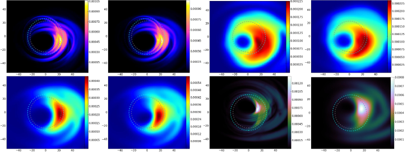
Figure 18.— Progression of BH shadow image plane intensity plots for SANE_dipole-jet model. From top-left to bottom-right, the progression shows: 1) single observer time at same time, same inclination $i=50^{\circ}$, same temperature prescription of $T_{i}/T_{e}=3$, similar mass accretion rate, and similar colormap compared to Dexter et al. (2010) ; 2) time-averaged over 10-minute interval using 8 snapshots (shows little difference) ; 3) colormap, inclination of $i=45^{\circ}$, and temperature prescription of fixed $T_{i}/T_{e}=10$ like for model D in Mościbrodzka et al. (2009); 4) our default time chosen instead (little difference); 5) our temperature prescription with $T_{\rm e,jet}=T_{\rm e,gas}$ (i.e., no isothermal jet); 6) our final temperature prescription with isothermal jet; 7) our best-fit for all parameters (e.g. inclination and density); and 8) including scattering. In each case, if required, the density was slightly changed to reproduce the $230$GHz zero baseline flux. This progression shows how color map choices, physical choices (inclination, temperature prescriptions), and scattering (at half the actual interstellar scattering, roughly what is possible by de-blurring after accounting for noise, see Fish et al. 2014; Lu et al. 2015; Chan et al. 2015b) affect whether the BH shadow appears detectable, suggesting that more quantitative measures of BH shadow detectability will be important to consider (Psaltis et al., 2015).

The shadows from other radiative transfer GRMHD models range from having a fairly low level of de-boosted emission (Dexter et al., 2010) to having a fairly bright de-boosted side (Mościbrodzka et al., 2014). These differences in GRMHD model results for the radiative transfer are controlled by differences in electron temperature prescriptions, mass accretion rates, and dynamical model differences.

We can highlight how some model choices affect the appearance of the BH shadow. Fig. 18 shows a progression of total-intensity images for the SANE_dipole-jet model. We start with a model that is similar to the model MBD described in Dexter et al. (2010) by using the same dynamical simulation, same inclination, same temperature prescription, and similar mass accretion rate. Although the radiative transfer codes are independent, they produce similar images (as expected), which exhibit a relatively pronounced shadow feature. We then introduce changes that eventually lead to our fiducial parameters for this model (see Table 1). In addition to being sensitive to the viewing inclination, temperature prescription, and assumptions about scattering mitigation, Fig. 18 shows that even the type of color map used can tend to imply the shadow is more detectable, because some color maps highlight low-level features so they can be seen visually (e.g. the so-called “jet” color map has this feature). As Fig. 18 also demonstrates, simply analyzing raw unscattered images sets unrealistic expectations for how the shadow may appear in EHT images. Compared to prior work, the final model shown in Fig. 18 reflects minor changes in the radiative transfer and realistic scattering limitations that generate a broad crescent feature that is both one-sided and partially filled-in.

Another origin of differences in simulation model results for the BH shadow could be due to the choice of initial conditions and run-time. Many prior simulations have initial conditions of a torus that lead to relatively thin disks with height-to-radius ratio of $H/R\lesssim 0.2$, while long-term GRMHD simulations evolved with a mass supply at large radii show radiatively inefficient accretion flows (RIAFs) tend towards $H/R\sim 0.4$ (Narayan et al., 2012) or even thicker at $H/R\sim 1$ (McKinney et al., 2012). GRMHD simulations that start with an initial torus too close (pressure maximum within $100r_{g}$ or inflow equilibrium within $30r_{g}$) to the BH remain controlled by those initial conditions, because the accretion process feeds off of the vertically thin torus material that has insufficient time to heat-up and become thick before reaching the BH. A thinner disk near the BH more readily produces a narrow sharp crescent (our SANE models happen to be run with tori with pressure maximum at $r\sim 10r_{g}$), while geometrically thick RIAFs with coronae tend to have a broad fuzzy crescent (our MAD models).

By comparison, analytical models can sometimes show a sharper photon ring and crescent-like feature (Broderick & Loeb, 2006; Broderick et al., 2009), because they tend to only include disk emission and no corona or jet emission that would broaden the crescent in a way dependent upon the temperature prescription. For example, the vertical structure assumed in Broderick et al. (2009) is that of a Gaussian with $H/R\sim 1$ for the disk, while hot coronae or jets have an extended column of gas that may not change the density scale-height much but change the emission profile to be more vertically extended. However, even the crescent feature in Broderick et al. (2009) is incomplete and shows little Doppler de-boosted emission one might need in order to clearly measure a shadow size. Further, analytical RIAF solutions like the advection-dominated accretion flow (ADAF) model have $H/R\sim 0.6$ or smaller for realistic prescriptions of the effective adiabatic index and any winds present (Quataert & Narayan, 1999a, b), which would presumably lead to a change in the BH shadow feature.

In summary, the filling-in of the BH shadow by corona or jet emission (as considered for GRMHD simulation-based radiative transfer models), and the broadening of the expected crescent feature by accretion flow structure and scattering may make it difficult to unambiguously detect the BH shadow or to extract information about the space-time from its size and shape (Broderick et al., 2014; Psaltis et al., 2015; Johannsen et al., 2015) before the plasma physics and dynamical properties of the disk and jet are constrained. Improved techniques to detect the shadow will be important in order to handle the diverse array of possible accretion flow physics and to best account for the scattering. In addition, the BH shadow’s appearance in polarization and at higher frequencies ($349$GHz), where the blurring from scattering is $2.3$ times weaker, will help increase its detectability.

3.8. 349GHz & CP

Extending the capabilities of the EHT to higher frequencies increases the angular resolution, reduces blurring due to interstellar scattering, and probes the emission structure at lower optical depth. The image-integrated (total) flux density is comparable at 230 and 345 GHz Bower et al. (2015).

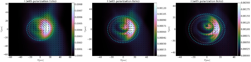
Figure 19.— Images at $230{\rm GHz}$ (left panel), $349{\rm GHz}$ (middle panel), and $674{\rm GHz}$ for the MAD_thick-jet model, which contains significant jet and coronal emission that fills-in the shadow at $230$GHz. As is similar for all our models, at higher frequencies, any emission in the central region begins to become optically thin and develops an intensity null, which is bounded by emission from the photon ring and some accretion material. Despite the presence of jet emission even at higher frequencies, the development of a null in intensity could be used to help detect the BH shadow.

Fig. 19 shows the MAD_thick-jet model and how the shadow feature becomes more distinguishable at higher frequencies. This revealing of the BH shadow (null in intensity bounded by emission) occurs because the surrounding emission structure becomes less opaque and less luminous at higher frequencies. Thus, even for underlying accretion models containing jet and corona emission, EHT data at $349{\rm GHz}$ can potentially detect the BH shadow. These results strongly motivate EHT efforts at $349{\rm GHz}$.

There are no CP data yet available from the EHT, but CP appears to differentiate magnetic field configurations, including among different MRI-type GRMHD models. For example, the SANE_dipole-jet model shows different circular polarization patterns in the visibility plane than the SANE_quadrupole-disk model, especially at long EHT baselines (see Figs. 6 and 7). Also, the visibility plane structure in $\breve{m}$ is quite different than the structure in $\breve{v}$, suggesting that linear and circular polarization each provide independent constraints on the underlying accretion flow structure. Higher sensitivity at higher frequencies may not be required for linear or circular polarization, which both increase with frequency.

4. Future Work

Validation of radiative transfer codes is crucial to ensure reliable comparisons are made between models and observations. Several codes exist to perform radiative transfer of GRMHD simulations during post-processing (Dexter et al., 2009; Mościbrodzka et al., 2009; Dexter et al., 2010; Mościbrodzka et al., 2014; Chan et al., 2015a, b). In section 3.7, we have compared our radiative transfer results with Dexter et al. (2010) for the same underlying simulation model and assumptions but using a different radiative transfer scheme, and we found reasonable qualitative agreement in the appearance of the shadow and overall emission structure in the image. In section 3.7, we have shown how even slight differences in color maps and physical assumptions lead to what looks like large changes in the appearance of the BH shadow. As more physics (such as polarization included in this paper, non-thermal particles, etc.) is considered, it will become crucial to ensure all radiative transfer codes can achieve the same quantitative and qualitative results for a suite of tests that include a diverse range of simulation and analytical models. In future work, we plan to compare the results of radiative transfer codes used by various researchers in the field.

In light of how EHT polarimetric observations offer a probe of models not possible with zero-baseline or non-polarimetric observations, we plan a more comprehensive investigation of a larger suite of GRMHD models beyond our models with relatively high spins. These include models which vary across a broad range of BH spins (McKinney et al., 2012) as well as models that vary across a broad range of tilt angles between the accretion disk angular momentum axis and BH spin axis (McKinney et al., 2013) (which should occur in Sgr A^∗and M87 on horizon scales, see Dexter & Fragile 2013; Polko & McKinney 2015). In order to better control emission from the funnel region, we will include new simulations that track the matter numerically-injected into the funnel to distinguish this material from self-consistently evolved material. In order to improve our ad hoc electron temperature prescriptions, we will include new simulations that track the electron and proton temperatures.

Currently, our fitting procedure does not include minimizing $\chi^{2}$ over image size or various nuisance parameters that modify the electron temperature or BZ-driven funnel jet mass-loading. Also, EVPA is not part of our zero baseline fitting procedure. Regarding the EHT, we only compare observations to simulation results, but we do not use that as part of our fitting procedure, so in principle SANE models might do better to match EHT observations in some part of our parameter space. We only compare EHT observations to simulations in linear polarization vs. intensity in the visibility plane, not focusing on EVPA and not focusing on CP that is not available yet. We provide some discussion of CP, because it is currently being measured by the EHT and some theoretical guidance is useful. Much more work on the radial extension of the disk model and any additional Faraday screens will be required to better fit zero-baseline CP and EVPA observations vs. frequency or any EHT data. For the GRMHD simulations used in this paper and any new simulations, in the future, we will also consider how zero-baseline EVPA and EHT measurements of CP and EVPA constrain the models. We will also consider closure phases and other similar diagnostics that are independent of visibility amplitudes and insensitive to single antenna phase errors (Doeleman et al., 2001; Broderick et al., 2011). CP, EVPA, and Faraday rotation can potentially probe the helical orientation of jet magnetic field (Contopoulos et al., 2009) or probe the degree of order of the disk magnetic field (Muñoz et al., 2012). The hope is that EHT CP and EVPA observations at non-zero baselines at $230$GHz or higher frequencies will further constrain the disk, jet, and plasma properties in unique ways compared to linear polarization fraction.

5. Conclusions

We have performed general relativistic (GR) polarized radiative transfer calculations on time-dependent three-dimensional GRMHD simulations to model thermal synchrotron emission from the Galactic Center source Sgr A^∗. We considered several models of MAD and SANE types with various kinetic-physics-inspired electron heating prescriptions that enhance the emission from the disk corona, funnel-wall jet that hugs the boundary between the disk and jet, and highly magnetized BZ-driven funnel jet.

We have compared our results to most recent (2013) polarimetry measurements by the EHT (Johnson et al., 2015b) and showed how polarization in the visibility (Fourier) domain distinguishes and constrains accretion flow models with different magnetic field structures. To identify which model would be favored, we compared a binned visibility amplitude ($\tilde{I}$) vs. binned visibility fractional linear polarization ($\breve{m}$), which the EHT can reliably measure (Johnson et al., 2015b). We also compared the simulation results for $\breve{m}$ vs. time for different baselines to see if the behavior matched the EHT observations. We focused on comparing to linear polarization at various (including zero) baseline lengths.

Our comparisons between the simulations and observations favor models with ordered magnetic fields near the event horizon in Sgr A^∗. Specifically, the MAD models are broadly consistent with these most recent EHT data sets for linear polarization fraction vs. intensity as well as linear polarization fraction vs. time. MADs occur when a supply of magnetic flux at larger distances accretes and accumulates near the BH. This leads to an ordered magnetic field threading the region around the horizon and threading the accretion disk near the photon orbit. For electron heating prescriptions that highlight emission from the disk (i.e., model MAD_disk), the emission that escapes to the observer primarily occurs from the disk near the photon orbit that is threaded by ordered poloidal magnetic field. For electron heating prescriptions that produce more jet emission (i.e., model MAD_jet), both the disk and funnel-wall jet contribute about equally. The agreement between the EHT data and MAD models is robust to fairly substantial changes in inclination angle.

The EHT observations disfavor the standard MRI-type SANE models with an initial dipolar field (i.e., model SANE_dipole-jet) more strongly than another MRI-type disk with an initial large-scale quadrupolar field (i.e., model SANE_quadrupole-disk). The former model contains a clear jet but contains mostly disordered magnetic field in the disk, while the latter model has no jet but contains ordered field within the disk. This suggests that, broadly speaking, those models with ordered magnetic fields threading the accretion disk are favored by the EHT data. The MAD models have the strongest degree of ordered dipolar magnetic field threading the accretion disk, causing them to be most like the EHT data and so favored over all other models. Even stronger constraints on the magnetic field structure should be possible with CP, EVPA, and higher ($349~{}{\rm GHz}$) frequencies.

We considered the BH shadow visually in the image plane and how it changes with different simulations and prescriptions for electron temperatures and BZ-driven funnel jet mass-loading. In general, the shadow feature is not necessarily distinct, e.g., it can be obscured by coronal emission from collisionless physics-inspired electron heating prescriptions, jet emission from sufficient jet mass-loading, and scattering. We have not performed a detailed analysis of the detectability of the BH shadow to validate what our visual inspection suggests. For some models with strong corona or jet emission at our fit-preferred inclinations, $349$GHz observations more readily reveal a BH shadow type null feature than $230$GHz. The BH shadow’s appearance in polarization should also increase its detectability, which we will consider in future work.

References

- Akiyama et al. (2015) Akiyama, K., Lu, R.-S., Fish, V. L., et al. 2015, ApJ, 807, 150
- Avara et al. (2015) Avara, M. J., McKinney, J. C., & Reynolds, C. S. 2015, ArXiv e-prints, arXiv:1508.05323
- Baganoff et al. (2003) Baganoff, F. K., Maeda, Y., Morris, M., et al. 2003, ApJ, 591, 891
- Balbus & Hawley (1998) Balbus, S. A., & Hawley, J. F. 1998, Reviews of Modern Physics, 70, 1
- Bardeen (1973) Bardeen, J. M. 1973, in Black Holes (Les Astres Occlus), ed. C. Dewitt & B. S. Dewitt (New York: Gordon and Breach), 215–239
- Beckwith et al. (2008) Beckwith, K., Hawley, J. F., & Krolik, J. H. 2008, ApJ, 678, 1180
- Blandford & Königl (1979) Blandford, R. D., & Königl, A. 1979, ApJ, 232, 34
- Blandford & Znajek (1977) Blandford, R. D., & Znajek, R. L. 1977, MNRAS, 179, 433
- Bower et al. (2015) Bower, G. C., Markoff, S., Dexter, J., et al. 2015, ApJ, 802, 69
- Brinkerink et al. (2015) Brinkerink, C. D., Falcke, H., Law, C. J., et al. 2015, ArXiv e-prints, arXiv:1502.03423
- Broderick et al. (2009) Broderick, A. E., Fish, V. L., Doeleman, S. S., & Loeb, A. 2009, ApJ, 697, 45
- Broderick et al. (2011) —. 2011, ApJ, 738, 38
- Broderick et al. (2014) Broderick, A. E., Johannsen, T., Loeb, A., & Psaltis, D. 2014, ApJ, 784, 7
- Broderick & Loeb (2006) Broderick, A. E., & Loeb, A. 2006, MNRAS, 367, 905
- Broderick & McKinney (2010) Broderick, A. E., & McKinney, J. C. 2010, ApJ, 725, 750
- Broderick & Tchekhovskoy (2015) Broderick, A. E., & Tchekhovskoy, A. 2015, ApJ, 809, 97
- Chan et al. (2015a) Chan, C.-k., Psaltis, D., Özel, F., et al. 2015a, ApJ, 812, 103
- Chan et al. (2015b) Chan, C.-K., Psaltis, D., Özel, F., Narayan, R., & Saḑowski, A. 2015b, ApJ, 799, 1
- Contopoulos et al. (2009) Contopoulos, I., Christodoulou, D. M., Kazanas, D., & Gabuzda, D. C. 2009, ApJ, 702, L148
- Dexter (2014) Dexter, J. 2014, in IAU Symposium, Vol. 303, IAU Symposium, ed. L. O. Sjouwerman, C. C. Lang, & J. Ott, 298–302
- Dexter et al. (2009) Dexter, J., Agol, E., & Fragile, P. C. 2009, ApJ, 703, L142
- Dexter et al. (2010) Dexter, J., Agol, E., Fragile, P. C., & McKinney, J. C. 2010, ApJ, 717, 1092
- Dexter & Fragile (2013) Dexter, J., & Fragile, P. C. 2013, MNRAS, 432, 2252
- Dexter et al. (2012) Dexter, J., McKinney, J. C., & Agol, E. 2012, MNRAS, 421, 1517
- Dodds-Eden et al. (2009) Dodds-Eden, K., Porquet, D., Trap, G., et al. 2009, ApJ, 698, 676
- Doeleman et al. (2009) Doeleman, S., Agol, E., Backer, D., et al. 2009, in Astronomy, Vol. 2010, astro2010: The Astronomy and Astrophysics Decadal Survey, 68
- Doeleman et al. (2001) Doeleman, S. S., Shen, Z.-Q., Rogers, A. E. E., et al. 2001, AJ, 121, 2610
- Doeleman et al. (2008) Doeleman, S. S., Weintroub, J., Rogers, A. E. E., et al. 2008, Nature, 455, 78
- Doeleman et al. (2012) Doeleman, S. S., Fish, V. L., Schenck, D. E., et al. 2012, Science, 338, 355
- Eckart et al. (2006a) Eckart, A., Schödel, R., Meyer, L., et al. 2006a, A&A, 455, 1
- Eckart et al. (2006b) Eckart, A., Baganoff, F. K., Schödel, R., et al. 2006b, A&A, 450, 535
- Falcke et al. (1998) Falcke, H., Goss, W. M., Matsuo, H., et al. 1998, ApJ, 499, 731
- Falcke & Markoff (2000) Falcke, H., & Markoff, S. 2000, A&A, 362, 113
- Falcke et al. (2000) Falcke, H., Melia, F., & Agol, E. 2000, ApJ, 528, L13
- Fish et al. (2013) Fish, V. L., Doeleman, S., Marrone, D. P., et al. 2013, in American Astronomical Society Meeting Abstracts, Vol. 221, American Astronomical Society Meeting Abstracts #221, #143.04
- Fish et al. (2009) Fish, V. L., Doeleman, S. S., Broderick, A. E., Loeb, A., & Rogers, A. E. E. 2009, ApJ, 706, 1353
- Fish et al. (2011) Fish, V. L., Doeleman, S. S., Beaudoin, C., et al. 2011, ApJ, 727, L36
- Fish et al. (2014) Fish, V. L., Johnson, M. D., Lu, R.-S., et al. 2014, ApJ, 795, 134
- Foucart et al. (2015) Foucart, F., Chandra, M., Gammie, C. F., & Quataert, E. 2015, ArXiv e-prints, arXiv:1511.04445
- Gammie et al. (2003) Gammie, C. F., McKinney, J. C., & Tóth, G. 2003, ApJ, 589, 444
- Gammie et al. (2004) Gammie, C. F., Shapiro, S. L., & McKinney, J. C. 2004, ApJ, 602, 312
- Genzel et al. (2010) Genzel, R., Eisenhauer, F., & Gillessen, S. 2010, Reviews of Modern Physics, 82, 3121
- Genzel et al. (2003) Genzel, R., Schödel, R., Ott, T., et al. 2003, Nature, 425, 934
- Ghez et al. (2008) Ghez, A. M., Salim, S., Weinberg, N. N., et al. 2008, ApJ, 689, 1044
- Globus & Levinson (2013) Globus, N., & Levinson, A. 2013, Phys. Rev. D, 88, 084046
- Howes et al. (2008) Howes, G. G., Dorland, W., Cowley, S. C., et al. 2008, Physical Review Letters, 100, 065004
- Igumenshchev et al. (2003) Igumenshchev, I. V., Narayan, R., & Abramowicz, M. A. 2003, ApJ, 592, 1042
- Johannsen et al. (2015) Johannsen, T., Broderick, A. E., Plewa, P. M., et al. 2015, ArXiv e-prints, arXiv:1512.02640
- Johnson & Quataert (2007) Johnson, B. M., & Quataert, E. 2007, ApJ, 660, 1273
- Johnson et al. (2014) Johnson, M. D., Fish, V. L., Doeleman, S. S., et al. 2014, ApJ, 794, 150
- Johnson & Gwinn (2015) Johnson, M. D., & Gwinn, C. R. 2015, ApJ, 805, 180
- Johnson et al. (2015a) Johnson, M. D., Loeb, A., Shiokawa, H., Chael, A. A., & Doeleman, S. S. 2015a, ApJ, 813, 132
- Johnson et al. (2015b) Johnson, M. D., Fish, V. L., Doeleman, S. S., et al. 2015b, Science, 350, 1242
- Komissarov & McKinney (2007) Komissarov, S. S., & McKinney, J. C. 2007, MNRAS, 377, L49
- Levinson et al. (2005) Levinson, A., Melrose, D., Judge, A., & Luo, Q. 2005, ApJ, 631, 456
- Lu et al. (2015) Lu, R.-S., Roelofs, F., Fish, V. L., et al. 2015, ArXiv e-prints, arXiv:1512.08543
- Luminet (1979) Luminet, J.-P. 1979, A&A, 75, 228
- Lynn et al. (2014) Lynn, J. W., Quataert, E., Chandran, B. D. G., & Parrish, I. J. 2014, ApJ, 791, 71
- Mahadevan & Quataert (1997) Mahadevan, R., & Quataert, E. 1997, ApJ, 490, 605
- Marrone et al. (2008) Marrone, D. P., Baganoff, F. K., Morris, M. R., et al. 2008, ApJ, 682, 373
- McKinney (2005) McKinney, J. C. 2005, ApJ, 630, L5
- McKinney (2006) —. 2006, MNRAS, 368, 1561
- McKinney & Blandford (2009) McKinney, J. C., & Blandford, R. D. 2009, MNRAS, 394, L126
- McKinney et al. (2015) McKinney, J. C., Dai, L., & Avara, M. J. 2015, MNRAS, 454, L6
- McKinney & Gammie (2004) McKinney, J. C., & Gammie, C. F. 2004, ApJ, 611, 977
- McKinney & Narayan (2007) McKinney, J. C., & Narayan, R. 2007, MNRAS, 375, 513
- McKinney et al. (2012) McKinney, J. C., Tchekhovskoy, A., & Blandford, R. D. 2012, MNRAS, 423, 3083
- McKinney et al. (2013) —. 2013, Science, 339, 49
- McKinney et al. (2014) McKinney, J. C., Tchekhovskoy, A., Sadowski, A., & Narayan, R. 2014, MNRAS, 441, 3177
- McKinney & Uzdensky (2012) McKinney, J. C., & Uzdensky, D. A. 2012, MNRAS, 419, 573
- Mościbrodzka & Falcke (2013) Mościbrodzka, M., & Falcke, H. 2013, A&A, 559, L3
- Mościbrodzka et al. (2015) Mościbrodzka, M., Falcke, H., & Shiokawa, H. 2015, ArXiv e-prints, arXiv:1510.07243
- Mościbrodzka et al. (2014) Mościbrodzka, M., Falcke, H., Shiokawa, H., & Gammie, C. F. 2014, A&A, 570, A7
- Mościbrodzka et al. (2011) Mościbrodzka, M., Gammie, C. F., Dolence, J. C., & Shiokawa, H. 2011, ApJ, 735, 9
- Mościbrodzka et al. (2009) Mościbrodzka, M., Gammie, C. F., Dolence, J. C., Shiokawa, H., & Leung, P. K. 2009, ApJ, 706, 497
- Mościbrodzka et al. (2012) Mościbrodzka, M., Shiokawa, H., Gammie, C. F., & Dolence, J. C. 2012, ApJ, 752, L1
- Muñoz et al. (2012) Muñoz, D. J., Marrone, D. P., Moran, J. M., & Rao, R. 2012, ApJ, 745, 115
- Narayan et al. (2003) Narayan, R., Igumenshchev, I. V., & Abramowicz, M. A. 2003, PASJ, 55, L69
- Narayan et al. (2012) Narayan, R., Sa̧dowski, A., Penna, R. F., & Kulkarni, A. K. 2012, MNRAS, 426, 3241
- Narayan & Yi (1994) Narayan, R., & Yi, I. 1994, ApJ, 428, L13
- Özel et al. (2000) Özel, F., Psaltis, D., & Narayan, R. 2000, ApJ, 541, 234
- Penna et al. (2010) Penna, R. F., McKinney, J. C., Narayan, R., et al. 2010, MNRAS, 408, 752
- Philippov et al. (2015) Philippov, A. A., Cerutti, B., Tchekhovskoy, A., & Spitkovsky, A. 2015, ArXiv e-prints, arXiv:1510.01734
- Polko & McKinney (2015) Polko, P., & McKinney, J. C. 2015, ArXiv e-prints, arXiv:1512.07969
- Psaltis et al. (2015) Psaltis, D., Özel, F., Chan, C.-K., & Marrone, D. P. 2015, ApJ, 814, 115
- Quataert & Gruzinov (1999) Quataert, E., & Gruzinov, A. 1999, ApJ, 520, 248
- Quataert & Gruzinov (2000) —. 2000, ApJ, 545, 842
- Quataert & Narayan (1999a) Quataert, E., & Narayan, R. 1999a, ApJ, 516, 399
- Quataert & Narayan (1999b) —. 1999b, ApJ, 520, 298
- Reid (2009) Reid, M. J. 2009, International Journal of Modern Physics D, 18, 889
- Ressler et al. (2015) Ressler, S. M., Tchekhovskoy, A., Quataert, E., Chandra, M., & Gammie, C. F. 2015, MNRAS, 454, 1848
- Ricarte & Dexter (2015) Ricarte, A., & Dexter, J. 2015, MNRAS, 446, 1973
- Riquelme et al. (2012) Riquelme, M. A., Quataert, E., Sharma, P., & Spitkovsky, A. 2012, ApJ, 755, 50
- Riquelme et al. (2015) Riquelme, M. A., Quataert, E., & Verscharen, D. 2015, ApJ, 800, 27
- Roberts et al. (1994) Roberts, D. H., Wardle, J. F. C., & Brown, L. F. 1994, ApJ, 427, 718
- Schödel et al. (2011) Schödel, R., Morris, M. R., Muzic, K., et al. 2011, A&A, 532, A83
- Shafee et al. (2008) Shafee, R., McKinney, J. C., Narayan, R., et al. 2008, ApJ, 687, L25
- Sharma et al. (2006) Sharma, P., Hammett, G. W., Quataert, E., & Stone, J. M. 2006, ApJ, 637, 952
- Sharma et al. (2007) Sharma, P., Quataert, E., & Stone, J. M. 2007, ApJ, 671, 1696
- Shcherbakov (2014) Shcherbakov, R. V. 2014, ASTRORAY: General relativistic polarized radiative transfer code, Astrophysics Source Code Library, ascl:1407.007
- Shcherbakov & Huang (2011) Shcherbakov, R. V., & Huang, L. 2011, MNRAS, 410, 1052
- Shcherbakov & McKinney (2013a) Shcherbakov, R. V., & McKinney, J. C. 2013a, ApJ, 774, L22
- Shcherbakov & McKinney (2013b) —. 2013b, ApJ, 774, L22
- Shcherbakov et al. (2012a) Shcherbakov, R. V., Penna, R. F., & McKinney, J. C. 2012a, ApJ, 755, 133
- Shcherbakov et al. (2012b) —. 2012b, ApJ, 755, 133
- Takahashi (2004) Takahashi, R. 2004, ApJ, 611, 996
- Tchekhovskoy & McKinney (2012) Tchekhovskoy, A., & McKinney, J. C. 2012, MNRAS, 423, L55
- Tchekhovskoy et al. (2007) Tchekhovskoy, A., McKinney, J. C., & Narayan, R. 2007, MNRAS, 379, 469
- Tchekhovskoy et al. (2010) Tchekhovskoy, A., Narayan, R., & McKinney, J. C. 2010, ApJ, 711, 50
- Tchekhovskoy et al. (2011) —. 2011, MNRAS, 418, L79
- Yuan et al. (2002) Yuan, F., Markoff, S., & Falcke, H. 2002, A&A, 383, 854
- Yuan & Narayan (2014) Yuan, F., & Narayan, R. 2014, ARA&A, 52, 529
- Yuan et al. (2003) Yuan, F., Quataert, E., & Narayan, R. 2003, ApJ, 598, 301
- Yuan et al. (2004) —. 2004, ApJ, 606, 894
- Yusef-Zadeh et al. (2008) Yusef-Zadeh, F., Wardle, M., Heinke, C., et al. 2008, ApJ, 682, 361