The Optical Activity of the Dark Exciton

Abstract

We present a phenomenological model to consider the effect of shape symmetry breaking on the optical properties of self-assembled quantum dots. We compare between quantum dots with two-fold rotational and two reflections ($C_{2v}$) symmetry and quantum dots in which this symmetry is reduced by perturbation to one reflection only ($C_{s}$). We show that this symmetry reduction drastically affects the optical activity of the dark exciton. In symmetric quantum dots, one of the dark exciton eigenstate is totally dark and the other, due to heavy- and light-hole mixing, has a small dipole moment polarized along the symmetry axis (growth direction) of the quantum dot. In non-symmetric quantum dots, the two dark excitons’ eigenstates are mixed with the bright excitons’ eigenstates which have cross-linearly polarized perpendicular to the growth direction dipole moments. As a result of this mixing one of the dark exciton eigenstate is dark while the other one does have dipole moment which is linearly polarized normal to the growth direction, like the lower energy bright exciton eigenstate. Our model agrees well with recently obtained experimental data.

I Introduction

Excitons in single semiconductor quantum dots (QDs) play a central role in many schemes for applications in quantum optics and future quantum technologies Loss and DiVincenzo (1998). QD confined excitons are generated by promoting one electron from the QD full valence band to the QD empty conduction band. If the electron spin is not altered in the process the generated excitons is optically active and it is called a bright exciton (BE). If however, the promoted electron spin is flipped (for example, during relaxation following non-resonant excitation) a dark exciton (DE), which is predominantly optically inactive, is formed. Since BEs are the fundamental optical excitations of these nanostructures they have been thoroughly studied both experimentally and theoretically. Their optical and coherent properties are quite well understood. Studies of DEs, which are as abundant as BEs in non-resonantly excited QDs, however, are relatively scarce. Recently, it was demonstrated that QD-confined DEs, despite their very weak optical activity, can still be efficiently accessed optically and electrically. Poem et al. (2010); Schwartz et al. (2015a, b) Moreover, it was demonstrated that DEs form long lived two-level spin systems Poem et al. (2010) with very long coherence times Schwartz et al. (2015a). These naturally neutral, non-degenerate two level systems form matter qubits with obvious advantages Schwartz et al. (2015a) over the single carrier spin qubits. It is therefore, important to study the DEs properties more thoroughly and to develop means for better understanding and thereby better controlling their properties.

In a recent publication Zieliński, Don, and Gershoni (2015) we used an atomistic model for studying the effect of QDs shape symmetry reduction on the optical properties of confined DEs in these QDs. We showed in Ref. Zieliński, Don, and Gershoni (2015) that the deviation from symmetry, effectively mixes the DE states with the states of the BE. The mixing results in increased optical activity of the DEs, in agreement with recent experimental observations. Atomistic models, however, are very detailed, they consume time and large computing resources and usually produce results which are far from being intuitively understood.

Here we develop a simple, phenomenological model for studying the effect of the deviation from symmetry on the DE properties. We show that despite its simplicity, our model does capture the essence of the symmetry reduction induced BE-DE mixing. It thereby provides an intuitive analytical tool for quantitative studies of QD confined DEs.

Theoretical studies of the fine structure of the confined exciton in semiconductor quantum dots (QDs) epitaxially grown on $[001]$ oriented substrate generally assume combined lattice and structural symmetry of $C_{2v}$ (i. e., symmetry under rotations of $\pi$ radians around the structural symmetry axis $[001]$, and under two reflections about perpendicular planes which contain the symmetry axis: the $[110]\textrm{--}[001]$ and the $[1\bar{1}0]\textrm{--}[001]$ planes. Ivchenko (2005); Takagahara (2000); Gupalov, Ivchenko, and Kavokin (1998). Since the quantum size effect and the strain result in large energy difference between the heavy-holes with total angular momentum projection $\pm 3/2$ on the symmetry axis and the light-holes with total angular momentum projection of $\pm 1/2$, the lowest energy exciton states are composed mainly of four different angular momentum configurations of electron hole pairs. Two exciton states, in which the electron and the heavy-hole have parallel angular momentum projections $\ket{+2},\ket{-2}$ with vanishing dipole matrix to optical transitions, called dark excitons (DEs); and two states, in which their spin projections are antiparallel, $\ket{+1},\ket{-1}$, forming the fundamental optical excitations of the QD, and therefore termed bright excitons (BEs).

General theoretical considerations, based on group theory arguments, imply that excitons in semiconductor nanostructures of $C_{2v}$ symmetry have four lowest energy eigenstates. Two of which have cross-linearly in-plane polarized dipole moments, associated with the two planes of reflection. One eigenstate have dipole moment polarized along the vertical symmetry axis ($\hat{z}$ direction, or $[001]$), and one eigenstate, which is completely dark. The first two eigenstates are associated with the bright excitons, while the later two are associated with the dark excitons. Ivchenko and Pikus (1997); Dupertuis et al. (2011) More specific considerations, which take into account the nature of the valence band structure in semiconductors, show that the $[001]$ polarized optical activity of one of the DE eigenstates and the lack of activity of the other eigenstate are attributed to constructive and destructive contributions to their dipole moments, respectively, due to heavy-light hole mixing. Takagahara (2000); Lovett et al. (2005)

Below, motivated by recent experimental observations, we construct a simple model which quantitatively account for the changes in the optical activity of the DE induced by small deviations from the exact $C_{2v}$ symmetry.

II Theoretical Model and Calculations

The electron hole exchange part of the Coloumb interaction removes the degeneracy between the 4 lowest exciton states. From general symmetry considerations, it can be shown that for $C_{2v}$ QDs the exchange interaction Hamiltonian written in the base $\ket{+1},\ket{-1},\ket{+2},\ket{-2}$ has the following form Ivchenko (2005); Takagahara (2000); Gupalov, Ivchenko, and Kavokin (1998):

$$\mathcal{H}_{C_{2v}}=\frac{1}{2}\begin{pmatrix}\Delta_{0}&\Delta_{1}^{*}&0&0\\ \Delta_{1}&\Delta_{0}&0&0\\ 0&0&-\Delta_{0}&\Delta_{2}^{*}\\ 0&0&\Delta_{2}&-\Delta_{0}\end{pmatrix}$$ (1)

Here $\Delta_{i},\,i=0,1,2$ are parameters that one either measures Alon-Braitbart et al. (2006); Bayer et al. (2002, 2000); Poem et al. (2010); Schwartz et al. (2015a) or try to calculate using simplified models Ivchenko and Pikus (1997); Ivchenko (2005); Gupalov, Ivchenko, and Kavokin (1998); Poem et al. (2007).

For a $C_{2v}$ symmetrical QD there is no mixing between the DEs and the BEs eigenstates. The two subspaces are energetically separated by $\Delta_{0}$. The parameter $\Delta_{1}$, which removes the degeneracy between the two BE states, is closely related to the oscillator strength for optical transitions to these fundamental excitations Poem et al. (2007); Takagahara (2000). For instance, using the envelope function approximation $\Delta_{1}$ is given by Takagahara (2000)

$$\tfrac{1}{2}\Delta_{1}=\Bra{\Phi_{\mathrm{h}}^{\Uparrow}\left(\mathbf{r}_{1}\right)\Phi_{\mathrm{e}}^{\downarrow}\left(\mathbf{r}_{2}\right)}\tfrac{e^{2}}{\epsilon}\tfrac{\boldsymbol{\mu}_{\downarrow\Uparrow}^{\dagger}\left(I-3\hat{n}\otimes\hat{n}^{\dagger}\right)\boldsymbol{\mu}_{\uparrow\Downarrow}}{\left|\mathbf{r}_{1}-\mathbf{r}_{2}\right|^{3}}$$ (2)

$$\Ket{\Phi_{\mathrm{e}}^{\uparrow}\left(\mathbf{r}_{1}\right)\Phi_{\mathrm{h}}^{\Downarrow}\left(\mathbf{r}_{2}\right)}$$

where $\epsilon$ is the dielectric constant, $e$ is the electronic charge, $\Phi_{\mathrm{e(h)}}^{s_{\mathrm{e}}(s_{\mathrm{h}})}$ is the electron (heavy-hole) conduction-band (valence-band) envelope function with spin $s_{\mathrm{e}}\left(s_{\mathrm{h}}\right)$, $\mathbf{r}_{1}$, $\mathbf{r}_{2}$ are the two carriers position vectors, $\hat{n}$ is a unit vector in the direction of $\mathbf{r}_{1}-\mathbf{r}_{2}$, $I$ is the $3\times 3$ unit matrix, $\hat{n}\otimes\hat{n}^{\dagger}$ a dyadic product, and $\boldsymbol{\mu}_{s_{\mathrm{e}}s_{\mathrm{h}}}$ is the valence-conduction band dipole matrix element.

The relation between the dipole matrix element and the momentum matrix element is given by Poem et al. (2007); Takagahara (2000)

$$\boldsymbol{\mu}_{s_{e}s_{h}}=\frac{-\mathrm{i}\hbar}{m_{0}E_{g}}\mathbf{M}_{s_{e}s_{h}}$$ (3)

where $E_{g}$ is the bandgap energy. The momentum matrix elements are Ivchenko (2005); Takagahara (2000)

$$\mathbf{M}_{\downarrow\Uparrow} =\tfrac{\mathrm{i}}{2}\sqrt{m_{0}E_{P}}\left(1,-\mathrm{i},0\right)$$ (4a)

$$\mathbf{M}_{\uparrow\Downarrow} =\tfrac{\mathrm{i}}{2}\sqrt{m_{0}E_{P}}\left(1,\mathrm{i},0\right)$$ (4b)

$$\mathbf{M}_{\uparrow\Uparrow}=\mathbf{M}_{\downarrow\Downarrow} =0$$ (4c)

where $E_{P}$ is Kane’s energy. Takagahara (2000)

$\Delta_{1,2}$ are in general complex numbers Ivchenko (2005) and can be expressed as $\Delta_{1,2}=\delta_{1,2}\mathrm{e}^{2\mathrm{i}\theta_{1,2}}$, where $\delta_{1,2}$ are positive numbers. Thus the eigenvalues of the Hamiltonian are expressed as

$$E_{\mathrm{BE}_{\pm}} =\tfrac{1}{2}(\Delta_{0}\pm\delta_{1})$$ (5a)

$$E_{\mathrm{DE}_{\pm}} =\tfrac{1}{2}(-\Delta_{0}\pm\delta_{2})$$ (5b)

and the eigenvectors as

$$v_{\mathrm{BE}_{\pm}} =\frac{1}{\sqrt{2}}\begin{pmatrix}\mathrm{e^{-i\theta_{1}}}\\ \pm\mathrm{e^{i\theta_{1}}}\end{pmatrix}$$ (6a)

$$v_{\mathrm{DE}_{\pm}} =\frac{1}{\sqrt{2}}\begin{pmatrix}\mathrm{e^{-i\theta_{2}}}\\ \pm\mathrm{e^{i\theta_{2}}}\end{pmatrix}$$ (6b)

Using the expressions for the momentum matrix element in Eqs. (4a) and (4b) one finds that the positive ($v_{\mathrm{BE_{+}}}$) and negative ($v_{\mathrm{BE_{-}}}$) eigenstates of the BE have dipole matrix elements linearly polarized along the $(\cos\theta_{1},-\sin\theta_{1},0)$ and $(\sin\theta_{1},\cos\theta_{1},0)$ directions, respectively, where $\theta_{1}$ is measured from the $[100]$ crystallographic direction.

Atomistic calculations Korkusinski and Hawrylak (2013); Zieliński, Don, and Gershoni (2015) and accumulated experimental data Young et al. (2005); Langbein et al. (2004); Bimberg, Grundmann, and Ledentsov (1999); Schwartz et al. (2015a) imply that most often the lowest (highest) energy BE emission spectral line is polarized along the $[1\bar{1}0]$ ($[110]$) direction, even for a circularly symmetric QD. If one defines the lowest energy line polarization as horizontal polarization (i.e symmetrical superposition of right and left hand circular polarizations) this situation is described by $\theta_{1}=135^{\circ}$.

The value of $\Delta_{2}$ is mostly determined by the short range e-h exchange interaction Ivchenko and Pikus (1997) which has the symmetry of the unit cell. This implies that $\Delta_{2}$ must be a real number Bayer et al. (2002), thus compelling $\theta_{2}$ to be either $0^{\circ}$ or $90^{\circ}$. Atomistic model simulations Zieliński, Don, and Gershoni (2015); Bryant et al. (2010), as well as recent experimental data Schwartz et al. (2015a) indicate that $\theta_{2}=90^{\circ}$.

From Eq. (4c) it follows that the DEs are completely dark. However, if one allows some residual heavy-hole light-hole mixing it follows that one of the DE eigenstates has small $\hat{z}$-polarized dipole moment, while the other one is totally dark Ivchenko and Pikus (1997); Ivchenko (2005); Dupertuis et al. (2011). Realistic atomistic model calculations of InAs/GaAs self assembled QDs indeed result with 3–6 orders of magnitude weaker $\hat{z}$-polarized optical activity of one of the DE eigenstate and a much weaker activity of the other DE eigenstate Korkusinski and Hawrylak (2013); Zieliński (2013); Smoleński et al. (2012); Zieliński, Don, and Gershoni (2015).

In reality, ideally symmetrized systems of macroscopic scale are extremely rare. Recent theoretical studies of epitaxial growth of strained heterostructures Spencer and Tersoff (2013) show that indeed self-assembled QDs can actually grow highly asymmetrical, largely deviating from $C_{2v}$ symmetry. In an asymmetrical QD, the subspaces of the BEs and DEs are no longer separated and their eigenstates are mixed Bayer et al. (2002).

In order to methodically study the effects of the structural symmetry reduction of the QD on the excitons, in our recent work Zieliński, Don, and Gershoni (2015) we used atomistic model, in which an inclined planar facet was introduced between the QD and the covering host material, thereby reducing the symmetry of the QD. As a result of the symmetry reduction both the electron and the hole have non-vanishing in-plane spin projection expectation values, where for a $C_{2v}$ symmetrical QD these expectation values vanish.

Here, we model the symmetry reduction by introducing a small angle $\varphi$ by which the symmetry axis of the QD is tilted relative to the $[001]$ crystallographic direction. As a result, the quantization axis of the QD potential is no longer aligned with the underlying semiconductor lattice, which defines the momentum matrix elements in Eq. (4). The electron (heavy-hole) envelope wavefunction’s symmetry axis is therefore inclined by an angle $\varphi_{\mathrm{e}}$ ($\varphi_{\mathrm{h}}$) relative to the $[001]$ crystallographic direction. Effectively, the new projections of the carrier spins on the envelope wavefunctions symmetry axes are given by:

$$\begin{pmatrix}\tilde{\uparrow}\\ \tilde{\downarrow}\end{pmatrix} =\begin{pmatrix}\cos\varphi_{\mathrm{e}}&\sin\varphi_{\mathrm{e}}\\ -\sin\varphi_{\mathrm{e}}&\cos\varphi_{\mathrm{e}}\end{pmatrix}\begin{pmatrix}\uparrow\\ \downarrow\end{pmatrix}$$ (7a)

$$\begin{pmatrix}\tilde{\Uparrow}\\ \tilde{\Downarrow}\end{pmatrix} =\begin{pmatrix}\cos\varphi_{\mathrm{h}}&\sin\varphi_{\mathrm{h}}\\ -\sin\varphi_{\mathrm{h}}&\cos\varphi_{\mathrm{h}}\end{pmatrix}\begin{pmatrix}\Uparrow\\ \Downarrow\end{pmatrix}$$ (7b)

As a result the matrix elements of Eqs. (4) transform to

$$\mathbf{M}_{\widetilde{\downarrow\Uparrow}} =+\mathbf{M}_{\downarrow\Uparrow}\cos\varphi_{\mathrm{e}}\cos\varphi_{\mathrm{h}}-\mathbf{M}_{\uparrow\Downarrow}\sin\varphi_{\mathrm{e}}\sin\varphi_{\mathrm{h}}$$ (8a)

$$\mathbf{M}_{\widetilde{\uparrow\Downarrow}} =-\mathbf{M}_{\downarrow\Uparrow}\sin\varphi_{\mathrm{e}}\sin\varphi_{\mathrm{h}}+\mathbf{M}_{\uparrow\Downarrow}\cos\varphi_{\mathrm{e}}\cos\varphi_{\mathrm{h}}$$ (8b)

$$\mathbf{M}_{\widetilde{\uparrow\Uparrow}} =+\mathbf{M}_{\downarrow\Uparrow}\sin\varphi_{\mathrm{e}}\cos\varphi_{\mathrm{h}}+\mathbf{M}_{\uparrow\Downarrow}\cos\varphi_{\mathrm{e}}\sin\varphi_{\mathrm{h}}$$ (8c)

$$\mathbf{M}_{\widetilde{\downarrow\Downarrow}} =-\mathbf{M}_{\downarrow\Uparrow}\cos\varphi_{\mathrm{e}}\sin\varphi_{\mathrm{h}}-\mathbf{M}_{\uparrow\Downarrow}\sin\varphi_{\mathrm{e}}\cos\varphi_{\mathrm{h}}$$ (8d)

Using only first order terms in $\varphi_{e}$ and $\varphi_{h}$ these equations become

$$\mathbf{M}_{\widetilde{\downarrow\Uparrow}} =\mathbf{M}_{\downarrow\Uparrow}$$ (9a)

$$\mathbf{M}_{\widetilde{\uparrow\Downarrow}} =\mathbf{M}_{\uparrow\Downarrow}$$ (9b)

$$\mathbf{M}_{\widetilde{\uparrow\Uparrow}} =\mathbf{M}_{\downarrow\Uparrow}\cdot\varphi_{\mathrm{e}}+\mathbf{M}_{\uparrow\Downarrow}\cdot\varphi_{\mathrm{h}}$$ (9c)

$$\mathbf{M}_{\widetilde{\downarrow\Downarrow}} =-\left(\mathbf{M}_{\downarrow\Uparrow}\cdot\varphi_{\mathrm{h}}+\mathbf{M}_{\uparrow\Downarrow}\cdot\varphi_{\mathrm{e}}\right)$$ (9d)

By adding and subtracting Eq. (9d) to and from Eq. (9c) one gets:

$$\mathbf{M}_{\widetilde{\uparrow\Uparrow}}+\mathbf{M}_{\widetilde{\downarrow\Downarrow}} =(\mathbf{M}_{\downarrow\Uparrow}-\mathbf{M}_{\uparrow\Downarrow})\cdot(\varphi_{\mathrm{e}}-\varphi_{\mathrm{h}})$$ (10a)

$$\mathbf{M}_{\widetilde{\uparrow\Uparrow}}-\mathbf{M}_{\widetilde{\downarrow\Downarrow}} =(\mathbf{M}_{\downarrow\Uparrow}+\mathbf{M}_{\uparrow\Downarrow})\cdot(\varphi_{\mathrm{e}}+\varphi_{\mathrm{h}})$$ (10b)

Eqs. (10) imply that the symmetric (antisymmetric) DE eigenstate is coupled only to the anti-symmetric (symmetric) BE eigenstate and that the coupling constant is proportional to $\varphi_{\mathrm{e}}-\varphi_{\mathrm{h}}$ ($\varphi_{\mathrm{e}}+\varphi_{\mathrm{h}}$).

We proceed by using Eq. (2), which associates the momentum matrix elements with the long range exchange interaction mixing term $\Delta_{1}$, to obtain the non-diagonal mixing terms between the BE and DE eigenstates of the Hamiltonian of a $C_{2v}$ QD as expressed by Eqs. (5) and (6). Substituting the modified momentum matrix elements of Eqs. (10) into Eq. (2) one gets the following modified Hamiltonian:

$$\mathcal{H}^{\prime}_{C_{s}}=\frac{1}{2}\begin{pmatrix}\Delta_{0}+\delta_{1}&0&\delta_{1}\cdot\left(\varphi_{\mathrm{h}}-\varphi_{\mathrm{e}}\right)&0\\ 0&\Delta_{0}-\delta_{1}&0&\delta_{1}\cdot\left(\varphi_{\mathrm{h}}+\varphi_{\mathrm{e}}\right)\\ \delta_{1}\cdot\left(\varphi_{\mathrm{h}}-\varphi_{\mathrm{e}}\right)&0&-\Delta_{0}+\delta_{2}&0\\ 0&\delta_{1}\cdot\left(\varphi_{\mathrm{h}}+\varphi_{\mathrm{e}}\right)&0&-\Delta_{0}-\delta_{2}\end{pmatrix}$$ (11)

This Hamiltonian can be expressed in terms of the original base $\ket{+1},\ket{-1},\ket{+2},\ket{-2}$:

$$\mathcal{H}_{C_{s}}=\frac{1}{2}\begin{pmatrix}\Delta_{0}&\delta_{1}\mathrm{e^{-2i\theta_{1}}}&\mathrm{i}\delta_{1}\mathrm{e^{-i\theta_{1}+i\theta_{2}}}\cdot\varphi_{\mathrm{h}}&-\mathrm{i}\delta_{1}\mathrm{e^{-i\theta_{1}-i\theta_{2}}}\cdot\varphi_{\mathrm{e}}\\ \delta_{1}\mathrm{e^{2i\theta_{1}}}&\Delta_{0}&-\mathrm{i}\delta_{1}\mathrm{e^{i\theta_{1}+i\theta_{2}}}\cdot\varphi_{\mathrm{e}}&\mathrm{i}\delta_{1}\mathrm{e^{i\theta_{1}-i\theta_{2}}}\cdot\varphi_{\mathrm{h}}\\ -\mathrm{i}\delta_{1}\mathrm{e^{i\theta_{1}-i\theta_{2}}}\cdot\varphi_{\mathrm{h}}&\mathrm{i}\delta_{1}\mathrm{e^{-i\theta_{1}-i\theta_{2}}}\cdot\varphi_{\mathrm{e}}&-\Delta_{0}&\delta_{2}\mathrm{e^{-2i\theta_{2}}}\\ \mathrm{i}\delta_{1}\mathrm{e^{i\theta_{1}+i\theta_{2}}}\cdot\varphi_{\mathrm{e}}&-\mathrm{i}\delta_{1}\mathrm{e^{-i\theta_{1}+i\theta_{2}}}\cdot\varphi_{\mathrm{h}}&\delta_{2}\mathrm{e^{2i\theta_{2}}}&-\Delta_{0}\end{pmatrix}$$ (12)

The new eigenenergies and eigenvectors of the reduced symmetry Hamiltonian of Eq. (11) are now:

$$E_{1}=\tfrac{+\delta_{1}-\delta_{2}}{4}+\tfrac{1}{2}\sqrt{\bigl{(}\tfrac{2\Delta_{0}+\delta_{1}+\delta_{2}}{2}\bigr{)}^{2}+\delta_{1}^{2}\bigl{(}\varphi_{\mathrm{h}}-\varphi_{\mathrm{e}}\bigr{)}^{2}}, \quad v_{1}=N_{1}\Bigl{(}\tfrac{2\Delta_{0}+\delta_{1}+\delta_{2}}{2\delta_{1}\left(\varphi_{\mathrm{h}}-\varphi_{\mathrm{e}}\right)}+\sqrt{\bigl{(}\tfrac{2\Delta_{0}+\delta_{1}+\delta_{2}}{2\delta_{1}\left(\varphi_{\mathrm{h}}-\varphi_{\mathrm{e}}\right)}\bigr{)}^{2}+1},0,1,0\Bigr{)}$$ (13a)

$$E_{2}=\tfrac{-\delta_{1}+\delta_{2}}{4}+\tfrac{1}{2}\sqrt{\bigl{(}\tfrac{2\Delta_{0}-\delta_{1}-\delta_{2}}{2}\bigr{)}^{2}+\delta_{1}^{2}\bigl{(}\varphi_{\mathrm{h}}+\varphi_{\mathrm{e}}\bigr{)}^{2}}, \quad v_{2}=N_{2}\Bigl{(}0,\tfrac{2\Delta_{0}-\delta_{1}-\delta_{2}}{2\delta_{1}\left(\varphi_{\mathrm{h}}+\varphi_{\mathrm{e}}\right)}+\sqrt{\bigl{(}\tfrac{2\Delta_{0}-\delta_{1}-\delta_{2}}{2\delta_{1}\left(\varphi_{\mathrm{h}}+\varphi_{\mathrm{e}}\right)}\bigr{)}^{2}+1},0,1\Bigr{)}$$ (13b)

$$E_{3}=\tfrac{-\delta_{1}+\delta_{2}}{4}-\tfrac{1}{2}\sqrt{\bigl{(}\tfrac{2\Delta_{0}-\delta_{1}-\delta_{2}}{2}\bigr{)}^{2}+\delta_{1}^{2}\bigl{(}\varphi_{\mathrm{h}}-\varphi_{\mathrm{e}}\bigr{)}^{2}}, \quad v_{3}=N_{3}\Bigl{(}\tfrac{2\Delta_{0}-\delta_{1}-\delta_{2}}{2\delta_{1}\left(\varphi_{\mathrm{h}}-\varphi_{\mathrm{e}}\right)}-\sqrt{\bigl{(}\tfrac{2\Delta_{0}-\delta_{1}-\delta_{2}}{2\delta_{1}\left(\varphi_{\mathrm{h}}-\varphi_{\mathrm{e}}\right)}\bigr{)}^{2}+1},0,1,0\Bigr{)}$$ (13c)

$$E_{4}=\tfrac{+\delta_{1}-\delta_{2}}{4}-\tfrac{1}{2}\sqrt{\bigl{(}\tfrac{2\Delta_{0}+\delta_{1}+\delta_{2}}{2}\bigr{)}^{2}+\delta_{1}^{2}\bigl{(}\varphi_{\mathrm{h}}+\varphi_{\mathrm{e}}\bigr{)}^{2}}, \quad v_{4}=N_{4}\Bigl{(}0,\tfrac{2\Delta_{0}+\delta_{1}+\delta_{2}}{2\delta_{1}\left(\varphi_{\mathrm{h}}+\varphi_{\mathrm{e}}\right)}-\sqrt{\bigl{(}\tfrac{2\Delta_{0}+\delta_{1}+\delta_{2}}{2\delta_{1}\left(\varphi_{\mathrm{h}}+\varphi_{\mathrm{e}}\right)}\bigr{)}^{2}+1},0,1\Bigr{)}$$ (13d)

where $N_{i}$ are normalization constants. Noting that $\Delta_{0}\gg\delta_{1}\gg\delta_{2}$ and $|\varphi_{\mathrm{e}}|,|\varphi_{\mathrm{h}}|\ll 1$, we may approximate those equations as:

$$E_{1}=\frac{+\Delta_{0}+\delta_{1}}{2}+\frac{\delta_{1}^{2}\bigl{(}\varphi_{\mathrm{h}}-\varphi_{\mathrm{e}}\bigr{)}^{2}}{4\Delta_{0}}, \qquad v_{1}=N_{-}\Bigl{(}1,0,+\frac{\delta_{1}\cdot\bigl{(}\varphi_{\mathrm{h}}-\varphi_{\mathrm{e}}\bigr{)}}{2\Delta_{0}},0\Bigr{)}$$ (14a)

$$E_{2}=\frac{+\Delta_{0}-\delta_{1}}{2}+\frac{\delta_{1}^{2}\bigl{(}\varphi_{\mathrm{h}}+\varphi_{\mathrm{e}}\bigr{)}^{2}}{4\Delta_{0}}, \qquad v_{2}=N_{+}\Bigl{(}0,1,0,+\frac{\delta_{1}\cdot\bigl{(}\varphi_{\mathrm{h}}+\varphi_{\mathrm{e}}\bigr{)}}{2\Delta_{0}}\Bigr{)}$$ (14b)

$$E_{3}=\frac{-\Delta_{0}+\delta_{2}}{2}-\frac{\delta_{1}^{2}\bigl{(}\varphi_{\mathrm{h}}-\varphi_{\mathrm{e}}\bigr{)}^{2}}{4\Delta_{0}}, \qquad v_{3}=N_{-}\Bigl{(}-\frac{\delta_{1}\cdot\bigl{(}\varphi_{\mathrm{h}}-\varphi_{\mathrm{e}}\bigr{)}}{2\Delta_{0}},0,1,0\Bigr{)}$$ (14c)

$$E_{4}=\frac{-\Delta_{0}-\delta_{2}}{2}-\frac{\delta_{1}^{2}\bigl{(}\varphi_{\mathrm{h}}+\varphi_{\mathrm{e}}\bigr{)}^{2}}{4\Delta_{0}}, \qquad v_{4}=N_{+}\Bigl{(}0,-\frac{\delta_{1}\cdot\bigl{(}\varphi_{\mathrm{h}}+\varphi_{\mathrm{e}}\bigr{)}}{2\Delta_{0}},0,1\Bigr{)}$$ (14d)

where $N_{\pm}$ are normalization constants.

To proceed, we now discuss the model angles $\varphi_{\mathrm{h}}$ and $\varphi_{\mathrm{e}}$, which for a $C_{\mathrm{2v}}$ symmetric QD are $\varphi_{\mathrm{e}}=\varphi_{\mathrm{h}}=0$. However, for a slightly lower symmetry QD ($C_{\mathrm{s}}$), the QD confined electron and hole are in their respective ground states, their envelope wavefunctions are typically restricted to the QD volume, and both possess the same in plane “$s$-like” symmetry. It is therefore expected that the respective angles of inclination between the electron and the hole envelope wavefunction symmetry axes and the crystallographic $[001]$ direction are similar. Both are approximately equal to $\varphi$: $\varphi_{\mathrm{h}}\simeq\varphi_{\mathrm{e}}\simeq\varphi$. By substituting the approximation $\varphi_{\mathrm{h}}=\varphi_{\mathrm{e}}\equiv\varphi$, in Eq. (11) one immediately sees that only the lower energy DE eigenstate acquires optical activity by mixing with the lower energy eigenstate of the BE. The dipole moment of this weakly visible DE eigenstate is thus polarized like that of the BE eigenstate, with which it is mixed ($H$-polarized), as indeed was recently observed experimentally Schwartz et al. (2015a). For a positive $\delta_{2}$ and $\theta_{2}=\frac{\pi}{2}$ this DE eigenstate is antisymmetric under electron-hole exchange, also in agreement with the experimental observation. Schwartz et al. (2015a) The energy and eigenvector of the visible DE are given by:

$$E_{4} \simeq\frac{-\Delta_{0}-\delta_{2}}{2}-\frac{\delta_{1}^{2}}{\Delta_{0}}\cdot\varphi^{2}$$ (15)

$$v_{4} \simeq\Bigl{(}0,\frac{-\delta_{1}\cdot\varphi}{\Delta_{0}},0,1\Bigr{)}$$

The calculated relative magnitude of the oscillator strength of the 4 exciton eigenstates as a function of the symmetry reduction $\varphi$ is presented in Fig. 1.

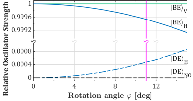
Figure 1: The calculated relative magnitude of the oscillator strength of the 4 exciton eigenstates (Eq. (11) for $\varphi_{\mathrm{h}}=\varphi_{\mathrm{e}}\equiv\varphi$). Solid $\mathrm{\ket{BE}_{V/H}}$ (dash $\mathrm{\ket{DE}_{H/NO}}$) lines represent BE (DE) eigenstates. Blue, green, and black colors represent $H$, $V$ polarizations, and no optical activity, respectively. The experimentally measured values of Ref. Schwartz et al. (2015a) are indicated by the magenta vertical line.

Our simple model can be readily compared with the recently measured experimental data of Ref. Schwartz et al. (2015a) where the visible DE to BE oscillator strength ratio of $\sim 5\times 10^{-4}$ is obtained at mixing strength of $\varphi=11^{\circ}$. The obtained angle agrees with the facet inclination angle of the atomistic model of Ref. Zieliński, Don, and Gershoni (2015).

If, however, the exciton is formed between electron and hole of different levels, the inclination angles $\varphi_{\mathrm{h}}$ and $\varphi_{\mathrm{e}}$ are not expected to be the same. Intuitively, one expects that the envelope wavefunction of a higher energy carrier, will be less restricted to the QD volume and thus less affected by the QD deviation from symmetry. Thus for example, for a DE between ground state electron and excited state heavy-hole one expects $|\varphi_{\mathrm{h}}|\ll|\varphi_{\mathrm{e}}|$. In this case, both DE eigenstates will be optically active with almost equal in plane polarized dipole moments, as indeed was recently observed experimentally. Schwartz et al. (2015b)

III Conclusions

We use a phenomenological model to examine the effects of symmetry reduction on the optical properties of the excitons in self assembled semiconductor QDs. We compare between excitons in $C_{2v}$ symmetrical QDs and excitons in QDs with small deviations from this symmetry. We model the symmetry reduction by an angle of inclination between the quantum dot symmetry axis and the crystallographic directions. We show that while the reduction in symmetry barely affects the bright exciton eigenstates and their optical activity, it strongly affects the optical activity of the dark exciton by mixing its eigenstates with these of the bright exciton. For the ground state dark exciton the lowest energy eigenstate has in-plane dipole moment which is polarized like the lowest energy bright exciton eigenstate, but the other eigenstate has much weaker optical activity. For excited dark exciton eigenstates this strong anisotropy in the in-plane dipole moment strengths is greatly reduced. The polarization selection rules, the oscillator strengths ratio, and the excitonic energy levels order, are well compared with recently measured data.