Depinning as a coagulation process

Abstract

We consider a one-dimensional sandpile model which mimics an elastic string of particles driven through a strongly pinning periodic environment with phase disorder. The evolution towards depinning occurs by the triggering of avalanches in regions of activity which are at first isolated but later grow and merge. For large system sizes the dynamically critical behavior is dominated by the coagulation of these active regions. Our analysis of the evolution and numerical simulations show that the observed sizes of active regions is well-described by a Smoluchowski coagulation equation, allowing us to predict correlation lengths and avalanche sizes.

Introduction —

Chains of particles connected by springs, where each particle experiences a randomly shifted periodic potential and an external driving force, have served as phenomenological models for charge density waves (CDWs) Grüner (1988); Fukuyama and Lee (1978). Of particular interest is the depinning transition as the external force increases to a threshold value beyond which the system slides, which is considered a dynamic critical phenomenon Fisher (1983, 1985); Littlewood (1986); Middleton and Fisher (1993); Myers and Sethna (1993); Coppersmith (1990); Coppersmith and Millis (1991). The behavior of such systems has been of interest in diverse areas, such as flux lines in type II superconductors Blatter et al. (1994), fluid invasion in porous media Wilkinson and Willemsen (1983), propagation of cracks Bouchaud et al. (2002); Alava et al. (2006), friction and earthquakes Kawamura et al. (2012), and plastic flows in solids, where dislocational structures depin under shear load Salman and Truskinovsky (2011, 2012). These systems being far from equilibrium, the mechanisms leading to critical behavior and universal features are not yet well-understood. This is due, at least in part, to a lack of simple models admitting detailed analysis.

The articles Kaspar and Mungan (2013, 2015) introduced one such model, a one-dimensional sandpile emerging in the strong pinning limit of a CDW system which may be driven along a transverse axis. When the external force varies slowly compared to the relaxation times, the evolution to threshold occurs by avalanches corresponding to the local depinning of segments. The resulting critical behavior is sensitive to initial conditions (ICs): starting from the final static configuration obtained driving in the $(-)$ direction, and then driving in the $(+)$ direction, the evolution towards threshold can be described explicitly and proceeds by the growth of a single depinned segment arrested only by its endpoints. The situation is markedly different when one considers generic ICs: the evolution proceeds by multiple depinned segments that each grow and merge. Numerics indicate Kaspar and Mungan (2013, 2015) that there is a critical transition, with different scaling behavior, agreeing with the predictions of Narayan et al. Narayan and Middleton (1994); Narayan and Fisher (1992). In this letter we report extensive simulation results concerning the evolution starting from a macroscopically flat initial condition. Our analysis reveals an unexpectedly clean connection with mean-field coagulation phenomena, providing a new viewpoint on macroscopic features of the depinning transition and shedding light on the emergence of universality in dynamical critical phenomena .

The model —

We begin by recalling the toy model of Kaspar and Mungan (2013, 2015). Fix a large integer $L$ and consider $L$-periodic vectors $\vec{z},\vec{m}$, and $\vec{\rho}$, related as follows:

$$z_{i}=\rho_{i}+\Delta m_{i}=\rho_{i}+m_{i-1}-2m_{i}+m_{i+1}.$$ (1)

Here $\vec{\rho}$ represents the quenched phase disorder, $\vec{m}$ counts the number of potential wells through which the particles are displaced, and $\vec{z}$ corresponds to a suitable rescaling of the displacements of the particles from the centers of their wells. Unlike the standard sandpile Bak et al. (1987); Dhar (1990); Redig (2006), heights $z_{i}$ have fractional parts from $\rho_{i}$ which persist, since the $m_{i}$ take only integer values, and the dynamics are deterministic and extremal Paczuski et al. (1996). The CDW process of raising the force until a particle crosses wells and waiting for the system to relax to a new static configuration is equivalent Kaspar and Mungan (2015) to applying the following avalanche algorithm:

• Record the critical height $h_{c}=\max_{i}z_{i}$.

• While there exists $i$ such that $z_{i}\geq h_{c}$, replace

  $$\begin{gathered}m_{i}\to m_{i}+1,\,z_{i}\to z_{i}-2,\,z_{i\pm 1}\to z_{i\pm 1}+1,\end{gathered}$$ (2)

  repeating as necessary until $\max_{i}z_{i}<h_{c}$.

This is precisely sandpile Dhar (1990) toppling at critical height $h_{c}$, and a standard argument Redig (2006) can be adapted to show that the result is independent of the order in which the indices $i$ are chosen in step A2. Furthermore, it can be shown Kaspar and Mungan (2015) that there is a unique number $z^{+}_{\max}$, the threshold height, such that the above algorithm terminates if and only if $h_{c}>z^{+}_{\max}$.

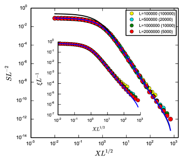
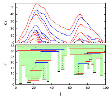
Figure 1: Left: finite-size scaling for avalanche size and correlation length (inset), including simulation data (circles) and predictions (curves; see (16)) for different system sizes $L$. Parenthesized numbers in the legend give the number of independent random realizations of the disorder. Top right: the evolution of well numbers $\vec{m}$ via avalanches for a small system of size $L=100$. Bottom right: the corresponding avalanche intervals and partitions, illustrating the active regions (ARs) of size $>1$ in light green. Both right: avalanches shown in black, red, and blue involve respectively 0, 1, and $\geq 2$ non-singleton ARs.

Define $i_{\max}=\operatorname{arg\,max}_{i}z_{i}$, when this is unique . Upon termination of the algorithm, $\vec{z}$ has changed by

$$\begin{gathered}\begin{aligned} z_{i_{\max}}&\to z_{i_{\max}}-1,&z_{i_{m}}&\to z_{i_{m}}-1\\ z_{i_{l}}&\to z_{i_{l}}+1,&z_{i_{r}}&\to z_{i_{r}}+1\end{aligned}\\ i_{m}=i_{r}+i_{l}-i_{\max}\end{gathered}$$ (3)

where $i_{l},i_{r}$ are the first sites to the left and right of $i_{\max}$ satisfying $z_{i}<h_{c}-1$, and $i_{m}$ is the reflection of $i_{\max}$ across the midpoint of the interval $i_{l},i_{r}$ Kaspar and Mungan (2015). (Above and henceforth all addition and subtraction of indices is to be understood modulo $L$, with results in $[0,L)$.) The change in $\Delta\vec{m}$ is the change in $\vec{z}$, so $\vec{m}$ is modified by adding a nonnegative trapezoidal bump with slopes $\{0,\pm 1\}$ and corners at $i_{l},i_{\max},i_{m},i_{r}$. We will refer to the periodic interval $[i_{l},i_{r}]$ as an avalanche segment. The length of the segment $i_{r}-i_{l}+1$ furnishes a correlation length $\xi$. Defining the size $\mathcal{S}$ of the avalanche as the total number of well jumps that occurred, it can be shown Kaspar and Mungan (2015) that $\mathcal{S}=(i_{\max}-i_{l})(i_{r}-i_{\max})$.

Observe that $z_{\max}$ decreases under repeated application of the algorithm. Let $\tau=0,1,2,\ldots$ index the observed configurations after $\tau$ complete executions of the algorithm, and define the control parameter $X$ as

$$X(\tau)=z_{\max}(\tau)-z^{+}_{\max}\geq 0.$$ (4)

We have $X(\tau)=0$ if, after $\tau$ avalanches, we reach the (essentially unique) threshold configuration with $z_{\max}=z_{\max}^{+}$, which gives the final shape of the chain prior to complete depinning. For the toy model this configuration can be explicitly constructed, yielding both a scaling limit for the threshold well numbers $\vec{m}^{+}$ as $L\to\infty$ and a characterization of the threshold force Kaspar and Mungan (2015).

Here we discuss the case of a flat initial configuration, $\vec{m}(0)=\vec{0}$, with disorder $\rho_{i}$ i.i.d. uniform on $[-1,+1]$, where the evolution to threshold is illustrated in Figure 1. The left panel shows the finite-size scaling behavior of the expected avalanche size $\mathcal{S}$ and correlation length $\xi$ obtained from extensive simulations, indicating that in the limit of large $L$, the depining transition is critical:

$$\mathcal{S}\sim X^{-\gamma}\quad\text{and}\quad\xi\sim X^{-\nu}\quad\text{with}\quad\gamma=4,\,\nu=2,$$ (5)

as predicted in Narayan and Middleton (1994); Narayan and Fisher (1992). The two panels on the right ilustrate the microscopic details of the evolution.

Coagulation —

Under repeated application of the avalanche algorithm, the flat initial configuration deforms via the depining of segments which are initially separated, but grow and merge. To understand this merging process, we define after each iteration of the algorithm a set of Active Regions (ARs) $\Pi(\tau)$. Each region is a periodic interval in $\{0,\ldots,L-1\}$, and we denote $[a,b]=\{a,a+1,\ldots,b\}$. Initially we have $\Pi(0)$ equal to the set of singleton intervals. The $\tau^{\mathrm{th}}$ avalanche occurs in some interval $[i_{l},i_{r}]$, and we define $\Pi(\tau)$ to be the finest partition of $\{0,\ldots,L-1\}$ which is coarser than the cover $\Pi(\tau-1)\cup\{[i_{l},i_{r}]\}$. More intuitively, the new partition joins together all those elements of the old partition which overlap with $[i_{l},i_{r}]$. Note that the set of endpoints of intervals in $\Pi(\tau)$ is exactly $\{i:m_{i}=0\}$. The ARs and their evolution are depicted by the light green shaded areas in Figure 1 (bottom right).

In associating with the dynamics the partitions $\Pi(\tau)$ as defined above, it seems that we have imposed coagulation on the problem, rasing the concern that the setup is contrived to yield the desired result. We emphasize the following Points:

• We do not require the coagulation to be binary, and yet will find that binary events are macroscopically dominant over a large portion of the evolution.

• The relative rates of coagulation events are not evident in the setup but rather will emerge, in one of the nicest possible forms, in both the numerics and a heuristic calculation.

• Each AR has at most one stop site which is pinned strongly enough to arrest avalanches.

• Since the avalanches which have occurred within the various active regions $\Pi(\tau)$ up to time $\tau$ have not interacted across the boundaries of $\Pi(\tau)$, we see that conditionally given $\Pi(\tau)$ we have

  $$(z_{i},m_{i}:i\in[a,b]),\quad[a,b]\in\Pi(\tau),$$ (6)

  statistically independent with distributions depending only on the sequence length $\ell=b-a+1$.

We proceed to explain P3 in detail. Suppose we have determined $h_{c}$ and completed an avalanche, resulting in the changes (3). The new configuration has $\vec{z}$ satisfying

$$h_{c}-2<z_{i_{m}}<h_{c}-1<z_{i}<h_{c},\quad\forall i\in[i_{l},i_{r}]\setminus\{i_{m}\}.$$ (7)

The first two inequalities hold because $i_{m}$ either did not initiate the avalanche and received $-1$, or $i_{m}=i_{\max}$ did initiate but received $-2$. The third holds because sites strictly between $i_{l}$ and $i_{r}$ were not capable of arresting the avalanche, and the sites $i_{l}$ and $i_{r}$ were capable but each received $+1$. We call $i_{m}$ a stop site because this is capable of halting (one side of) a subsequent avalanche avalanche above critical heights $h_{c}-\epsilon$ for some $\epsilon>0$. Stop sites may expire: before having the opportunity to stop an avalanche, the critical height might have decreased more than $\epsilon$. When an avalanche joins two or more ARs, $i_{l}$ and $i_{r}$ must land on unexpired stop sites, using them by adding $+1$ and creating a single new stop site inbetween. By induction each active region has at most one stop site. Note that by establishing (7), an avalanche conditions an AR’s response to future avalanches. This response is markedly different in pristine areas where no avalanches have yet occurred: after one side of an avalanche enters such an area, it will continue for a number of sites whose average admits a small $O(1)$ upper bound (independent of the system size) which holds uniformly over the whole evolution.

Mean-field statistics —

Our main observation is that the length statistics of the ARs recorded in $\Pi(\tau)$ are numerically quite close to a well-known Golovin (1963); Aldous (1999) exact solution

$$f(t,\ell)=e^{-t}B(1-e^{-t},\ell),\quad B(\lambda,\ell)=\frac{(\lambda\ell)^{\ell-1}e^{-\lambda\ell}}{\ell!},$$ (8)

to the Smoluchowski coagulation equation with additive collision kernel Smoluchowski (1916); Aldous (1999); Norris (1999):

$$\partial_{t}f(t,\ell)=\sum_{\ell^{\prime}=1}^{\ell-1}\frac{1}{2}\alpha(\ell^{\prime},\ell-\ell^{\prime})f(t,\ell^{\prime})f(t,\ell-\ell^{\prime})\\ -\sum_{\ell^{\prime}=1}^{\infty}\alpha(\ell,\ell^{\prime})f(t,\ell)f(t,\ell^{\prime}),$$ (9)

for $\ell=1,2,\ldots$, and in the additive case $\alpha(\ell,\ell^{\prime})=\ell+\ell^{\prime}$. This infinite-dimensional ODE system describes binary aggregation in the mean-field setting: $f(t,\ell)$ gives the number density per unit volume of clusters of size $\ell$ at time $t$, where clusters of sizes $\ell$ and $\ell^{\prime}$ interact to form a new cluster of size $\ell+\ell^{\prime}$ at rate $\alpha(\ell,\ell^{\prime})$. Equation (9), with various kernels $\alpha(\cdot,\cdot)$, has been used in modeling aerosols Drake (1972), formation of large scale structure in astronomy Silk and White (1978), and aggregation of algae cells Ackleh et al. (1994).

Associated with a realization of the toy model and its partitions $\Pi(\tau)$ of ARs we have a size distribution

$$N(\tau,\ell)=\sum_{[a,b]\in\Pi(\tau)}\delta_{b-a+1,\ell},$$ (10)

normalized so that $L^{-1}N(0,\ell)=f(0,\ell)=\delta_{\ell,1}$, using Kronecker $\delta$ notation. We give numerical evidence that $f$ approximates a law of large numbers for $N$ at fixed times $\tau$. For this we take many realizations, which we synchronize in time not by the number of steps $\tau$ but rather $X(\tau)$ defined in (4), which is the natural control parameter. Given a realization and $x\in[0,1]$, write $\vec{z}(x),\vec{m}(x)$ for the first configuration we observe with $X\leq x$, and likewise write $\Pi(x)$ for its associated partition into ARs. Given $R$ independent realizations with corresponding size distributions $N_{1}(x,\ell),\ldots,N_{R}(x,\ell)$, define

$$F_{R}(x,\ell)=(LR)^{-1}\sum_{k=1}^{R}N_{k}(x,\ell).$$ (11)

We obtain $F_{R}$ via simulation with a Python library we have developed for the toy model Kaspar and İşeri (2016). After matching time scales $x$ for $F_{R}$ and $t$ for $f$ by equating second moments,

$$\sum_{\ell}\ell^{2}F_{R}(x,\ell)=\sum_{\ell}\ell^{2}f(t,\ell)=e^{2t},$$ (12)

we plot in Figure 2 distributions $f(t,\ell)$ and $F_{R}(x,\ell)$ at various times.

Similarities explained —

We do not prove the law of large numbers suggested above, and indeed do not claim that this is exactly given by $f$, but can offer a heuristic Explanation of the similarities:

• The probability that the next avalanche begins with a site inside an AR of length $\ell$ is similar to $\ell/L$.

• Since large ARs will initiate avalanches most often, their stop sites will tend to be used rather than expire, and the avalanches mostly extend in only one direction.

• On the side where the avalanche exits the triggering AR, it is very likely to stop if it hits another macroscopically-sized AR. We thus expect to join to the triggering AR some small number of tiny ARs, which is not macroscopically observable, and (probably) at most one macrosocopic AR.

Combining E2 and E3, we expect that assuming binary coagulation yields a reasonable approximation when we care primarily about large ARs, as we will for the correlation length and avalanche size that we discuss shortly.

• Though the model is spatially ordered, statistically it behaves as if it is well mixed. In particular the length of the second AR in the avalanche is selected uniformly from the list of all AR lengths (excluding the triggering AR). We explain further below.

Assuming that E1–E4 hold and that the system is large enough that $N(\tau,\ell)$ is effectively deterministic, the expected change $N(\tau+1,\ell)-N(\tau,\ell)$ is approximated by

$$\sum_{\ell^{\prime}=1}^{\ell-1}\frac{\ell^{\prime}N(\tau,\ell^{\prime})}{L}\frac{N(\tau,\ell-\ell^{\prime})}{M_{0}(\tau)}-\frac{\ell N(\tau,\ell)}{L}-\frac{N(\tau,\ell)}{M_{0}(\tau)},$$ (13)

having written

$$M_{k}(\tau)=\sum_{\ell=1}^{L}\ell^{k}N(\tau,\ell)$$ (14)

for the $k^{\mathrm{th}}$ moment of $N$. The summation in (13) is over those sizes which sum to $\ell$, and reflects choosing a triggering AR with probability like $\ell^{\prime}/L$ and then a second AR uniformly from those which remain. The loss terms correspond to selection as a triggering AR or as a secondary AR. Symmetrizing the summation of (13) in the variables $\ell^{\prime},\ell-\ell^{\prime}$ and factoring $LM_{0}(\tau)$ yields an equation matching (9), up to a change in time scale.

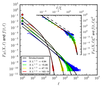
Figure 2: The empirical length distributions $F_{R}(X,\ell)$ (various colors) compared with the exact solution $f(t,\ell)$ to Smoluchowski (8), matching $X$ and $t$ by equating second moments. In the inset, the axes are scaled so that the these collapse; the dashed line is a power law with exponent $-3/2$ and follows from (8). The agreement of distributions deteriorates prior to and after the scaling region visible in Figure 1; see also the animation, available online İşeri (2016), which provides a dynamic view of the above. The colored markers placed at $\ell=1$ and the gap in the data between $\ell=1$ and $\ell=3$ are artifacts of the definition of the partition $\Pi$: we cannot produce any ARs of length 2.

Regarding E4, recall that the Smoluchowski equation arises as a law of large numbers for the Marcus-Lushnikov Marcus (1968); Lushnikov (1978) stochastic coalescent as the number of clusters tends to infinity Aldous (1999); Norris (1999); Rezakhanlou (2013); Fournier and Giet (2004); Cepeda and Fournier (2011). These models are well-mixed in the sense that any pair of clusters may interact, which contrasts with the toy model where ARs can interact only consecutively with some number of neighbors on each of the left and right. Nonetheless it is possible to remain well-mixed statistically with aggregating nearest-neighbor interactions : in the case of the toy model it can be shown that the partitions $\Pi(\tau)$, $\tau=0,1,2,\ldots$, are exchangeable in the sense that the vector of lengths

$$(b-a+1:[a,b]\in\Pi(\tau))$$ (15)

has a distribution which is invariant under permutations.

Observables and moments —

We present an example to show how this connection between depinning and coagulation can be exploited: certain observables are immediately related to the explicitly calculable moments of the solution to the Smoluchowski equation. Namely, supposing that the avalanche triggering sites and stop sites inside ARs are uniformly distributed, which is consistent with numerics for large ARs, we find expected length $\xi$ and size $\mathcal{S}$ of an avalanche as

$$\xi=\frac{2}{3}\frac{M_{2}}{M_{1}}+\frac{1}{2}\frac{M_{1}}{M_{0}}\quad\text{and}\quad\mathcal{S}=\frac{1}{12}\frac{M_{3}}{M_{1}}+\frac{1}{6}\frac{M_{2}}{M_{0}},$$ (16)

respectively. The blue curves in Figure 1 (left) plot the moment relations for $\mathcal{S}$ and $\xi$ from (16) using the statistics of the AR lengths obtained from our simulations. The black curve in the main panel is obtained by evaluating the moments $M_{i}$ using the exact solution (8). The agreement with simulations over the scaling regime is quite good, deteriorating close to threshold for the result based on the exact Smoluchowski solution. The main reason for this discrepancy is that the finite model admits clusters only as large as $L$, whereas no such restriction exists for the Smoluchowski equation. Using (8) and (16) in the scaling region, it is readily shown that $\mathcal{S}=\frac{9}{16}\xi^{2}$, which implies the scaling relation $\gamma=2\nu$; cf. (5).

Conclusion —

We have presented numerical evidence connecting depinning phenomena with coagulation, and finish with several reasons this relationship deserves further exploration. First, the toy model discussed in this letter is sufficiently tractable that we expect further analytical results should be attainable. For instance it may be possible to explicitly relate the various time scales $\tau$ and $X$ for the toy model and $t$ for the Smoluchowski equation, which would provide not only relations between $\xi$ and $\mathcal{S}$, as presented above, but also express these as functions of time. Second, though the model we discuss is considerably simplified, the essential features—aggregation of depinned segments (our ARs), avalanches which relieve load in a few localized interior areas (our stop sites) while increasing it at the boundaries—seem to be applicable to a broader class of pinning models. On a macroscopic level, depinning in these models would be expected to be still governed by a similar coagulation process. Third, combining the Brownian scaling limit result for the threshold configuration of Kaspar and Mungan (2015) with the observations in this letter may lead to a stochastic process describing the macroscopic limit of depinning in these models. The second and third points can provide an explanation for the emergence of universal features in such transitions.