Optical spectroscopy of molecular junctions: Nonequilibrium Green’s functions perspective

Abstract

We consider optical spectroscopy of molecular junctions from the quantum transport perspective when radiation field is quantized and optical response of the system is simulated as photon flux. Using exact expressions for photon and electronic fluxes derived within the nonequilibrium Green function (NEGF) methodology and utilizing fourth order diagrammatic perturbation theory in molecular coupling to radiation field we perform simulations employing realistic parameters. Results of the simulations are compared to the bare perturbation theory (PT) usually employed in studies on nonlinear optical spectroscopy to classify optical processes. We show that the bare PT violates conservation laws, while flux conserving NEGF formulation mixes optical processes.

I Introduction

The interaction of light with molecules is an important field of research due to its ability to provide information on molecular structure and dynamics, and to serve as a control tool for intra-molecular processes. Tremendous progress of laser technologies combined with advances in fabrication techniques opened the way to perform optical experiments on molecular conduction junctions. In particular, current induced fluorescence Wu et al. (2008), Raman scattering Ioffe et al. (2008); Ward et al. (2008, 2011), single-molecule imaging Chen et al. (2010), and optical probing of quantum charge fluctuations Schneider et al. (2012) were reported in the literature. Optical read-out of junction response to fast voltage pulses was recently utilized to enable access to transient processes at nanosecond timescale Grosse et al. (2013). Currently experiments are being developed to access molecular dynamics in junctions on the sub-picosecond timescale within pump-probe measurements Selzer and Peskin (2013); Ochoa et al. (2015). These advancements bring the fields of molecular electronics and optical spectroscopy together indicating emergence of molecular optoelectronics Galperin and Nitzan (2012).

Theory of nonlinear optical spectroscopy has been developed Mukamel (1995) and widely utilized in studies of optical response of molecules Okumura and Tanimura (1997a, b); Xu et al. (2001); Ovchinnikov et al. (2001); Okumura and Tanimura (2003); Mukamel et al. (2004); Šanda and Mukamel (2005); Yang and Mukamel (2008); Harbola and Mukamel (2009). In most spectroscopic applications radiation field is treated classically (with exception made in treatment of spontaneous emission processes), and the treatment relies on bare perturbative theory (PT) expansion in the molecule-field coupling which conveniently allows to classify different optical processes based on description of evolution of the system density matrix propagation in time while interacting with external field (both bra and ket interactions are distinguished by the treatment) Mukamel (1995). Application of these standard tools to description of optical response in molecular junctions was done in a number of publications Harbola et al. (2006, 2014); Goswami et al. (2015); Agarwalla et al. (2015) Radiation field was treated semi-classically in these works, hybridization between molecular and contacts states was disregarded. Optical spectroscopy of isolated molecules involving quantum description of the field was put forward in Refs. Rahav and Mukamel (2010); Mukamel and Rahav (2010). These studies consider optical processes from the viewpoint of the matter, where optical signals are recast in terms of transition amplitudes which represent the isolated molecule wave function. It was demonstrated that interference between optical paths involving different orders of the field must be taken into account in order to properly reproduce the flux of populations between different molecular states.

Biased molecular junctions are open quantum systems which exchange energy and particles with the contacts, and quantum description of optical field is often desirable in these systems (see, e.g., Ref. Lodahl et al. (2015) for recent review of quantum electrodynamics experiments at nanoscale). Nonequilibrium Green function (NEGF) formulation treating both quantum transport and optical response on the same footing was formulated in a set of publications Galperin et al. (2009a, b); Park and Galperin (2011a, b); Galperin and Nitzan (2011a, b); Oren et al. (2012); Banik et al. (2013); White et al. (2014); Galperin et al. (2015); Dey et al. (2016). These studies allow an accurate treatment of the coupling with electrodes and treat radiation field quantum mechanically. Following the standard nonlinear optical spectroscopy formulation they rely on bare PT expansion of the molecular coupling to radiation field. Note that perturbative treatment of the coupling is reasonable, because a realistic estimate of the interaction with the field is $\sim 10^{-3}-10^{-2}$ eV Sukharev and Galperin (2010), while for a molecule chemisorbed on metallic surface electronic escape rate, which characterizes the molecule-contact interaction, is $\sim 0.01-0.1$ eV Kinoshita et al. (1995).

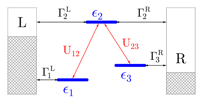
Figure 1: Optical spectroscopy in molecular junctions. Shown is a sketch of the model.

Here we discuss applicability of the standard nonlinear optical spectroscopy formulation to problems of optical response in current-carrying molecular junctions with the field treated quantum mechanically. We simulate electron and photon fluxes utilizing a simple model and employing realistic parameters. Our results show that violation of conservation laws by bare PT may be quite visible within realistic range of parameters. The conserving NEGF (diagrammatic perturbation theory) formulation Stefanucci and van Leeuwen (2013) involves resumming infinite series of diagrams which makes separation of the photon flux into contributions of different order in the field impossible. We stress that while below we consider steady-state and employ perturbation theory up to fourth order in molecule-field coupling, our conclusions are not limited by this choice. Indeed, requirement of self-consistency (resumming diagrams to infinite order) in constructing conserving approximations equally applicable to time-dependent processes, while any finite order subset is non-conserving Baym and Kadanoff (1961); Baym (1962).

Structure of the paper is as follows. In Section II we introduce a junction model and discuss a way to calculate its transport and optical response within diagrammatic perturbation theory. Section III compares this formulation to the bare PT treatment and shows similarities and differences of the two formulations. Numerical illustrations are presented and discussed in Section IV. Section V summarizes our findings.

II Model

We consider a junction consisting of molecule $M$ coupled to two metallic contacts $L$ and $R$ each at its own equilibrium. The junction is subjected to external radiation field which is treated quantum mechanically. We model the molecule as a three-level system with the levels corresponding to, e.g., two ground ($\varepsilon_{1}$ and $\varepsilon_{3}$) and one excited ($\varepsilon_{2}$) electronic states (see Fig. 1). Within the model level $\varepsilon_{1}$ is coupled to $L$ contact only, while $\varepsilon_{3}$ - to $R$ only. This may be viewed as a representation of states with strong charge-transfer transition Galperin and Nitzan (2005, 2006). Hamiltonian of the model is (here and below $e=\hbar=k_{B}=1$)

$$\hat{H}= \hat{H}_{0}+\hat{V}$$ (1)

$$\hat{H}_{0}= \sum_{m\in M}\varepsilon_{m}\hat{d}_{m}^{\dagger}\hat{d}_{m}+\sum_{k\in L,R}\varepsilon_{k}\hat{c}_{k}^{\dagger}\hat{c}_{k}+\sum_{\alpha}\omega_{\alpha}\hat{a}_{\alpha}^{\dagger}\hat{a}_{\alpha}$$ (2)

$$+ \sum_{m\in M}\sum_{k\in L,R}\left(V_{mk}\hat{d}_{m}^{\dagger}\hat{c}_{k}+H.c.\right)$$

$$\hat{V}= \sum_{m_{1},m_{2}\in M}\sum_{\alpha}\left(U_{\alpha,m_{1}m_{2}}\hat{a}_{\alpha}^{\dagger}\hat{D}_{m_{1}m_{2}}+H.c.\right)$$ (3)

Here $\hat{H}_{0}$ is the quadratic part of the Hamiltonian, while $\hat{V}$ characterizes coupling to radiation field. $\hat{d}_{m}^{\dagger}$ ($\hat{d}_{m}$) and $\hat{c}_{k}^{\dagger}$ ($\hat{c}_{k}$) create (annihilate) electron in the molecular level $m$ or level $k$ of the contacts, respectively. $\hat{D}_{m_{1}m_{2}}\equiv\hat{d}_{m_{1}}^{\dagger}\hat{d}_{m_{2}}$ is the molecular de-excitation operator. $\hat{a}_{\alpha}^{\dagger}$ ($\hat{a}_{\alpha}$) creates (annihilates) photon in the mode $\alpha$ of the radiation field. Contacts $L$ and $R$ are considered to be equilibrium reservoirs of electrons characterized by their electrochemical potentials, $\mu_{L}$ and $\mu_{R}$, and temperature $T$ common to both contacts. Radiation field is considered as continuum of modes. In the incoming field a mode around frequency $\omega_{0}$ is assumed to be populated with $N_{0}$ photons, all other modes of the field are empty.

We will be interested in calculating electron and photon fluxes in the junction. Within the NEGF the fluxes are defined as rates of change in the bath populations Haug and Jauho (2008); Galperin et al. (2007) (see also Appendix A for derivation)

$$I_{K}(t)\equiv\frac{d}{dt}\sum_{k\in K}\langle\hat{c}_{k}^{\dagger}(t)\hat{c}_{k}(t)\rangle$$ (4)

$$=2\,\mbox{Re}\int_{-\infty}^{t}dt^{\prime}\mbox{Tr}\bigg{[}\Sigma_{K}^{<}(t,t^{\prime})\,G^{>}(t^{\prime},t)-\Sigma_{K}^{>}(t,t^{\prime})\,G^{<}(t^{\prime},t)\bigg{]}$$

$$I_{pt}(t)\equiv\frac{d}{dt}\sum_{\alpha}\langle\hat{a}_{\alpha}^{\dagger}(t)\hat{a}_{\alpha}(t)\rangle$$ (5)

$$=2\,\mbox{Re}\int_{-\infty}^{t}dt^{\prime}\mbox{Tr}\bigg{[}\Pi^{<}(t,t^{\prime})\,F^{>}(t^{\prime},t)-\Pi^{>}(t,t^{\prime})\,F^{<}(t^{\prime},t)\bigg{]}$$

where $\mbox{Tr}[\dots]$ is trace over electronic levels in $M$ in (4) and radiation field modes in (5). $G^{\gtrless}$ and $F^{\gtrless}$ are greater/lesser projections of electron and photon Green functions ($T_{c}$ is the Keldysh contour ordering operator)

$$G_{mm^{\prime}}(\tau,\tau^{\prime})\equiv -i\langle T_{c}\,\hat{d}_{m}(\tau)\,\hat{d}_{m^{\prime}}^{\dagger}(\tau^{\prime})\rangle$$ (6)

$$F_{\alpha\alpha^{\prime}}(\tau,\tau^{\prime})\equiv -i\langle T_{c}\,\hat{a}_{\alpha}(\tau)\,\hat{a}_{\alpha^{\prime}}^{\dagger}(\tau^{\prime})\rangle$$ (7)

which satisfy the Dyson equations Haug and Jauho (2008)

$$G_{mm^{\prime}}(\tau,\tau^{\prime})=G^{(0)}_{mm^{\prime}}(\tau\tau^{\prime})+\sum_{m_{1},m_{2}}\int_{c}d\tau_{1}\int_{c}d\tau_{2}\,$$

$$\qquad G^{(0)}_{mm_{1}}(\tau,\tau_{1})\,\Sigma^{pt}_{m_{1}m_{2}}(\tau_{1},\tau_{2})\,G_{m_{2}m^{\prime}}(\tau_{2},\tau^{\prime})$$ (8)

$$F_{\alpha\alpha^{\prime}}(\tau,\tau^{\prime})=F^{(0)}_{\alpha\alpha^{\prime}}(\tau,\tau^{\prime})+\sum_{\alpha_{1},\alpha_{2}}\int_{c}d\tau_{1}\int_{c}d\tau_{2}\,$$

$$\qquad F^{(0)}_{\alpha\alpha_{1}}(\tau,\tau_{1})\,\Pi_{\alpha_{1}\alpha_{2}}(\tau_{1},\tau_{2})\,F_{\alpha_{2}\alpha^{\prime}}(\tau_{2},\tau^{\prime})$$ (9)

Here $G^{(0)}$ and $F^{(0)}$ are the Green functions propagated by the Hamiltonian $\hat{H}_{0}$, Eq. (2).

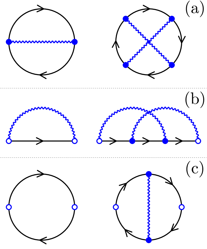
Figure 2: Diagrammatic perturbation theory. Shown are dressed skeleton diagrams of (a) the Luttinger-Ward generating functional, $\Phi$, and corresponding (b) electron, $\Sigma$, and (c) photon, $\Pi$, self-energies. Left diagrams correspond to second and right to fourth order contributions. Directed solid line (black) represents the electron Green function $G$, Eq. (6). Wavy line (blue) is the photon Green function $F$, Eq. (7); both directions are implied here. Empty and solid circles indicate outer and inner vertices. Summation over all degrees of freedom and integration over contour variables is done in the latter.

In Eqs. (6)-(II) $\Sigma_{K}$, $\Sigma^{pt}$ and $\Pi$ are the electron self-energy due to coupling to the contact $K$ ($L$ or $R$), electron self-energy due to coupling to radiation field, and photon self-energy due to coupling to electron-hole excitations in the molecule, respectively. $\Sigma_{K}$ is known exactly

$$\left[\Sigma_{K}(\tau,\tau^{\prime})\right]_{mm^{\prime}}=\sum_{k\in K}V_{mk}\,g_{k}(\tau,\tau^{\prime})\,V_{km^{\prime}}$$ (10)

Here $g_{k}$ is the Green function of free electrons in contact $K$. Thus coupling to the contacts, represented by second row in Eq.(2), is treated exactly. $\Sigma^{pt}$ and $\Pi$ can be derived only approximately. These approximations should be conserving, i.e. fulfill conservation laws for physical quantities (charge, momentum, energy, etc.). A way of formulating such approximations was established in the works by Kadanoff and Baym Baym and Kadanoff (1961); Baym (1962). Standard diagrammatic procedure requires construction of the Luttinger-Ward functional, $\Phi$ - the collection of all connected skeleton diagrams (i.e. diagrams that have no self-energy insertions) Luttinger and Ward (1960); De Dominicis and Martin (1964). Expressions for self-energies are obtained as functional derivatives Haussmann (1999); White and Galperin (2012); Stefanucci and van Leeuwen (2013)

$$\Sigma^{pt}_{mm^{\prime}}(\tau,\tau^{\prime})= \frac{\delta\Phi[G,F]}{\delta G_{m^{\prime}m}(\tau^{\prime},\tau)}$$ (11)

$$\Pi_{\alpha\alpha^{\prime}}(\tau,\tau^{\prime})= -\frac{\delta\Phi[G,F]}{\delta F_{\alpha^{\prime}\alpha}(\tau^{\prime},\tau)}$$ (12)

Figure 2a shows diagrams for $\Phi$ up to fourth order in electron-photon interaction $\hat{V}$, Eq.(3).

Corresponding diagrams for electron and photon self-energies are shown in Figs. 2b and c, respectively. Explicit expressions for the self-energies are given in Appendix B. Note that the self-energies, Eqs. (11) and (12), are expressed in terms of the full (or dressed) Green functions, Eqs. (6) and (11). The latter are obtained from the Dyson equations, Eqs. (II) and (II), which in turn depend on the self-energies. Thus, solution becomes a self-consistent procedure, and any conserving approximation requires resummation of an infinite number of diagrams.

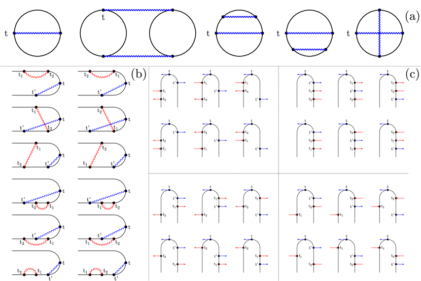
Figure 3: A contribution to photon flux $I_{pt}(t)$, Eq.(5), within fourth order bare PT expansion. Shown are (a) Diagrams contributing to the perturbative expression, (b) the Keldysh contour projections (physical time increases from left to right) and (b) corresponding double-sided Feynman diagrams (physical time increases from bottom to top). Straight lines in panel (a) indicate bare electron propagators, $G^{(0)}$. Wavy lines in panels (a) and (b) indicate bare photon propagators, $F^{(0)}$; Arrows in panel (c) indicate creation ($\hat{a}_{\alpha}^{\dagger}$, pointing to left) or annihilation ($\hat{a}_{\alpha}$, pointing to right) photon operators.

III The bare perturbative expansion

Traditionally treatment of system’s response to quantum field relies on calculating rate of change of a field mode occupation number (see Chapter 9 of Ref. Mukamel (1995)). This is the same definition of the photon flux within NEGF, Eq. (5). The rate is simulated utilizing bare PT in coupling to the field, Eq.(3), with second order contribution (called linear response) yielding absorption of a quantum field and fourth order contribution (called third order process) describing spontaneous light emission (SLE) spectroscopy Mukamel (1995). Perturbative expansion yields set of terms characterized by form of electronic correlation functions (evaluated in the absence of the field) which includes set of times indicating interaction with optical field. It is customary to represent each term as a double-sided Feynman diagram. The diagram shows times and side of the contour (bra or ket), where interaction with the field takes place (see Ref. Mukamel (1995) for details; examples of the double-sided Feynman diagrams are presented in Fig 3c).

We now consider the bare PT expressions for electron and photon fluxes, Eqs. (4) and (5), from the diagrammatic perturbation theory point of view Fetter and Walecka (1971); Mahan (1990). Fourth order perturbation theory (PT) contributions to photon flux, Eq.(5), are shown in Fig. 3a. Following classification of the diagrammatic perturbation theory the expansion contains contributions which can be divided into three groups: 1. disconnected diagrams, 2. reducible diagrams (2nd diagram in Fig. 3a), and 3. irreducible diagrams (diagrams 1, 3-5 in Fig 3a). According to diagrammatic technique the disconnected diagrams should be disregarded, because by the linked cluster theorem they cancel by corresponding contributions from the denominator (renormalization of the partition function) Fetter and Walecka (1971); Wagner (1991); Haussmann (1999). The reducible diagrams correspond to partial resummations of the photon Dyson equation. For example, utilizing $\sum_{\alpha_{1},\alpha_{2}}\int_{c}d\tau_{1}\int_{c}d\tau_{2}\,F^{(0)}_{\alpha\alpha_{1}}(\tau,\tau_{1})\,\Pi_{\alpha_{1}\alpha_{2}}(\tau_{1},\tau_{2})\,F^{(0)}_{\alpha_{2}\alpha^{\prime}}(\tau_{2},\tau^{\prime})$ instead of second term in the right of Eq.(II) (i.e. taking one of infinite number of terms in the Dyson equation) in expression for the photon flux, Eq.(5), will result in contribution to the flux corresponding to a reducible diagram (2nd diagram in Fig. 3a). The irreducible diagrams come from partial resummations of the electron Dyson equation and from expressions for the photon self-energy with Green functions $G$ and $F$ substituted with their bare counterparts $G^{(0)}$ and $F^{(0)}$. For example, utilizing bare photon Green function $F^{(0)}$ in expression for the photon flux, Eq.(5), and substituting in place of two electron Green functions in the expression for photon self-energy $\Pi^{(2)}$, Eq.(46), one bare Green function $G^{(0)}$, and bare version of second term Eq.(II), leads to bare irreducible diagrams in the SLE signal (third and fourth diagrams of Fig. 3a). Similarly, perturbative expansion of electron and photon Green functions $G$ and $F$ will enter also expressions for charge and energy currents (see Eqs. (13)-(18) below).

Absorption (linear response) is obtained by substituting bare photon Green function $F^{(0)}$ and bare version of $\Pi^{(2)}$, Eq.(46), into (5). SLE signal (third order process) is a sum of many contributions (fourth order bare diagrams) in (5), each of which contains two physical times, $t$ and $t^{\prime}$, and two contour variables, $\tau_{1}$ and $\tau_{2}$. The former are the times in the flux expression, Eq.(5), while the latter come either from bare version of second term in the Dyson equations, Eqs. (II) and (II) or bare versions of self-energies $\Sigma^{pt\,(2)}$ and $\Pi^{(4)}$, respectively Eqs. (44) and (47). Physical times $t$ and $t^{\prime}$ are fixed on the Keldysh contour with time $t$ (time of the flux) being the latest time. Contour variables $\tau_{1}$ and $\tau_{2}$ are projected (i.e. become physical times $t_{1}$ and $t_{2}$) by considering all possible placements (orderings) of the variables on the contour. Fig. 3b shows an example of all possible orderings for a contribution to the first term in Eq.(5).

The standard formulation Mukamel (1995) deals with the same problem of ordering variables $\tau_{1}$ and $\tau_{2}$ between the two times $t$ and $t^{\prime}$. However this time the ordering is performed along the real time axis (i.e. not only relative position of times on the contour but also relative position on the real time axis is tracked). Thus, number of different orderings, the double-sided Feynman diagrams, is larger here. It is customary to indicate each photon process by separate arrow in these orderings, rather than consider contractions representing free photon propagation. The agreement is that arrow pointing to the left corresponds to creation operator of the photon in quantum mechanical description of the field (or factor $e^{i\omega_{\alpha}t}$ for classical treatment of the field), while arrow pointing to the right represents operator of annihilation of the photon (or factor $e^{-i\omega_{\alpha}t}$) Mukamel (1995). Fig. 3c shows all possible double-sided Feynman diagrams corresponding to the Keldysh contour projection of Fig. 3b. Note that word ‘diagram’ has different meanings in the diagrammatic perturbation technique (particular combination of Green functions - see Fig. 3a) and in the bare PT expansion (particular ordering of contour times $\tau_{1}$ and $\tau_{2}$ - see Fig. 3b or c). In particular, each of many Green function arrangements will be characterized by the same set of time orderings. Note also that (as discussed in Section II) construction of a conserving approximation requires resummations of infinite series of diagrams of Fig. 3a. The latter will mix different bare orders making it impossible to distinguish between, say, absorption and SLE or introduce double-sided Feynman diagrams in a meaningful way (see also discussion in Ref. Caroli et al. (1972)). The total photon flux, Eq.(5), remains the only characteristic of optical response.

IV Numerical results

Here we present numerical simulations illustrating discussion in sections II and III. Simulations are performed for the molecular junction model of Fig. 1 performed at steady-state conditions. We compare the diagrammatic and bare PT approaches. At steady-state expressions for particle (electron and photon) fluxes, Eqs. (4) and (5), become

$$I_{K}= \int_{-\infty}^{+\infty}\frac{dE}{2\pi}\,i_{K}(E)$$ (13)

$$I_{pt}= \int_{-\infty}^{+\infty}\frac{d\omega}{2\pi}\,i_{pt}(\omega)$$ (14)

where $i_{K}(E)$ and $i_{pt}(\omega)$ are energy resolved electron and photon particle fluxes

$$i_{K}(E)\equiv \mbox{Tr}\bigg{[}\Sigma_{K}^{<}(E)\,G^{>}(E)-\Sigma_{K}^{>}(E)\,G^{<}(E)\bigg{]}$$ (15)

$$i_{pt}(\omega)\equiv \mbox{Tr}\bigg{[}\Pi^{<}(\omega)\,F^{>}(\omega)-\Pi^{>}(\omega)\,F^{<}(\omega)\bigg{]}$$ (16)

We will also calculate corresponding energy fluxes (energy exchanged between molecule and environment by electron and photon fluxes)

$$J_{K}\equiv \int_{-\infty}^{+\infty}\frac{dE}{2\pi}\,E\,i_{K}(E)$$ (17)

$$J_{pt}\equiv \int_{-\infty}^{+\infty}\,\frac{d\omega}{2\pi}\,\omega\,i_{pt}(\omega)$$ (18)

Expressions for the fluxes within the bare PT expansion are obtained from those above along the lines discussed in Section III.

Clearly, at steady state one expects conservation of charge

$$I_{L}=-I_{R}$$ (19)

and energy

$$J_{L}+J_{R}+J_{pt}=0$$ (20)

to be fulfilled. Below we illustrate that bare PT simulations violate these conservation laws.

Strength of the molecule-contacts interaction is characterized by the dissipation matrix

$$\Gamma_{mm^{\prime}}^{K}(E)\equiv 2\pi\sum_{k\in K}V_{mk}V_{km^{\prime}}\delta(E-\varepsilon_{k})$$ (21)

Lesser and greater projections of the self-energy (10), which yield respectively in- and out-scattering of electrons, are given by

$$\left[\Sigma^{<}_{K}(E)\right]_{mm^{\prime}}= i\Gamma^{K}_{mm^{\prime}}(E)\,f_{K}(E)$$ (22)

$$\left[\Sigma^{>}_{K}(E)\right]_{mm^{\prime}}= -i\Gamma^{K}_{mm^{\prime}}(E)\,[1-f_{K}(E)]$$ (23)

Lamb shift and dissipation are given by real and imaginary parts of the retarded projection

$$\left[\Sigma^{r}_{K}(E)\right]_{mm^{\prime}}=\Lambda_{mm^{\prime}}(E)-\frac{i}{2}\Gamma_{mm^{\prime}}(E)$$ (24)

which are related by the Kramers-Kronig expressions (i.e. either of the parts defines the other) Mahan (1990). Here $f_{K}(E)=[e^{(E-\mu_{K})/k_{B}T}+1]^{-1}$ is the Fermi-Dirac thermal distribution in contact $K$ (characterized by temperature $T$ and electrochemical potential $\mu_{K}$). In what follows we disregard cross-terms of the dissipation matrix $\Gamma^{K}_{mm^{\prime}}(E)$, Eq.(21) and consider only its diagonal terms $\Gamma^{K}_{m}\equiv\Gamma^{K}_{mm}$ (see Fig. 1). The latter are electronic escape rates. This is a reasonable assumption, when inter-level distance is much bigger than strength of the molecule-contacts coupling. Moreover, for simplicity we adopt the wide band approximation, which neglects the lamb shift, $\Lambda=0$, and assumes electronic escape rates to be energy-independent. Zero-order electronic Green functions projections are

$$G^{(0)\,<}_{mm^{\prime}}(E)= \delta_{m,m^{\prime}}\sum_{K\in L,R}\frac{i\Gamma^{K}_{m}f_{K}(E)}{(E-\varepsilon_{m})^{2}+(\Gamma_{m}/2)^{2}}$$ (25)

$$G^{(0)\,>}_{mm^{\prime}}(E)= \delta_{m,m^{\prime}}\sum_{K\in L,R}\frac{-i\Gamma^{K}_{m}[1-f_{K}(E)]}{(E-\varepsilon_{m})^{2}+(\Gamma_{m}/2)^{2}}$$ (26)

$$G^{(0)\,r}_{mm^{\prime}}(E)= \frac{\delta_{m,m^{\prime}}}{E-\varepsilon_{m}+i\Gamma_{m}/2}$$ (27)

where $\Gamma_{m}\equiv\sum_{K=L,R}\Gamma_{m}^{K}$ is the total escape rate from level $m$ of the molecule.

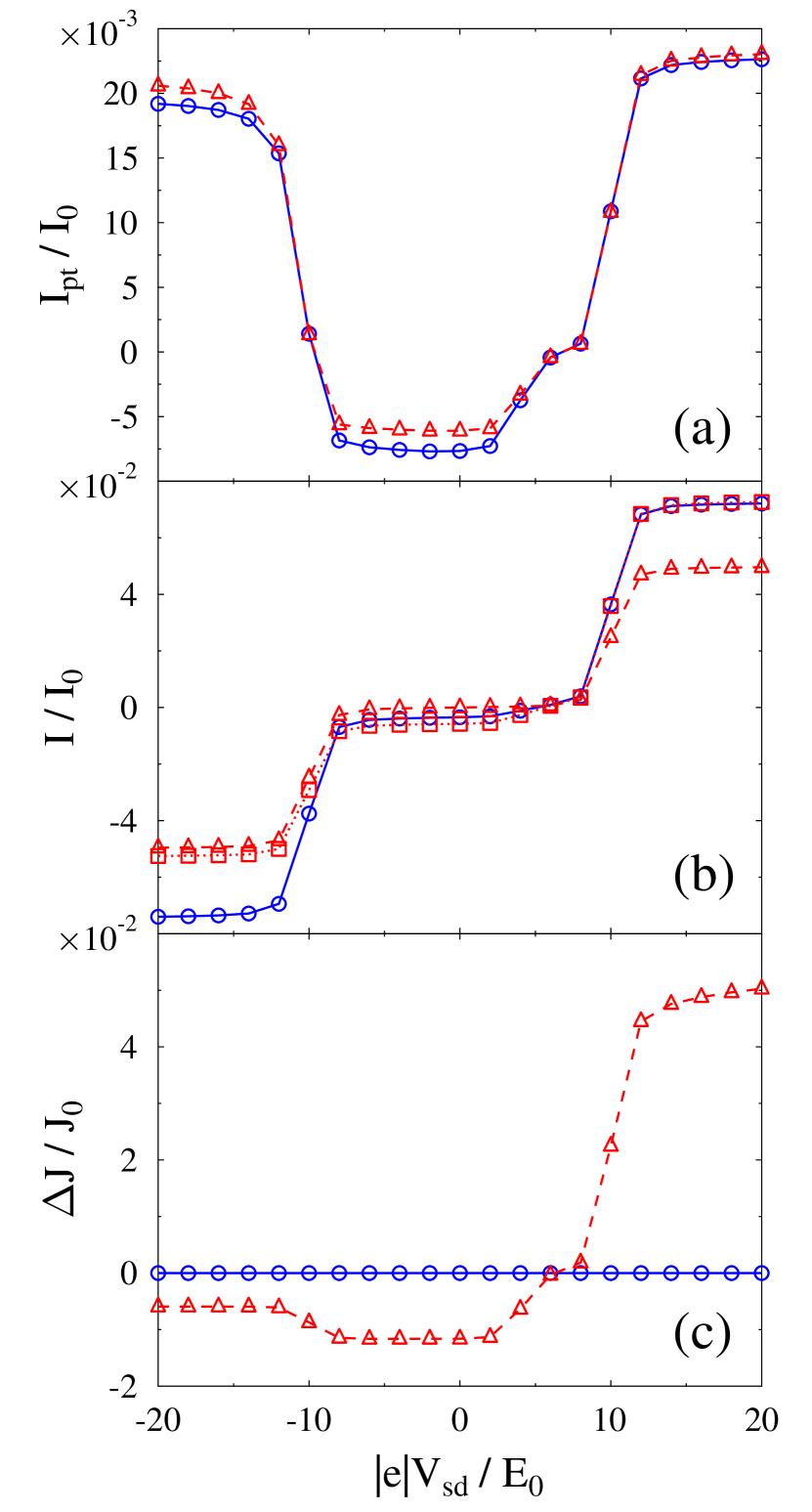
Figure 4: Transport and optical response of the molecular junction, Fig. 1, under applied bias $V_{sd}$. Steady-state self-consistent diagrammatic simulations (circles, solid blue line) are compared with bare PT results (triangles, dashed red line and squares, dotted red line). Shown are (a) Optical flux $I_{pt}$, Eq.(14); (b) current $I_{K}$, Eq.(13); and (c) deviation from conservation of energy, $\Delta J\equiv J_{L}+J_{R}+J_{pt}$. In panel (b) $I_{L}$ is shown with triangles and $-I_{R}$ with squares for the bare PT approach ($I_{L}=-I_{R}$ in the self-consistent simulation). See text for parameters.

Strength of molecular coupling to radiation field is described by the radiation dissipation tensor

$$\gamma_{m_{1}m_{2},m_{3}m_{4}}(\omega)\equiv 2\pi\sum_{\alpha}U_{m_{1}m_{2},\alpha}U_{\alpha,m_{3}m_{4}}\delta(\omega-\omega_{\alpha})$$ (28)

Within the model the tensor has four non-zero elements (see Fig. 1): $12,12$; $12,32$; $32,12$; and $32,32$. For simplicity we assume all the elements to be the same and given by the following expression

$$\gamma(\omega)=\gamma_{0}\bigg{(}\frac{\omega}{\omega_{C}}\bigg{)}^{2}e^{2(1-\omega/\omega_{C})}$$ (29)

where $\omega_{0}$ is the laser frequency. Instead of the photon GF $F_{\alpha\alpha^{\prime}}$ for each pair of modes $\alpha$ and $\alpha^{\prime}$, Eq. (7), in the simulations we consider Green function characterizing the whole radiation field

$$S_{m_{1}m_{2},m_{3}m_{4}}(\tau,\tau^{\prime})\equiv\sum_{\alpha,\alpha^{\prime}}U_{m_{1}m_{2},\alpha}\,F_{\alpha\alpha^{\prime}}(\tau,\tau^{\prime})\,U_{\alpha^{\prime},m_{3}m_{4}}$$ (30)

One can easily see that it satisfies the same Dyson equation, Eq. (II), with obvious modifications of the self-energy definitions. Its zero-order projections are

$$S^{(0)\,<}_{m_{1}m_{2},m_{3}m_{4}}(\omega)= -iN_{pt}(\omega)\,\gamma_{m_{1}m_{2},m_{3}m_{4}}(\omega)$$ (31)

$$S^{(0)\,>}_{m_{1}m_{2},m_{3}m_{4}}(\omega)= -i[1+N_{pt}(\omega)]\,\gamma_{m_{1}m_{2},m_{3}m_{4}}(\omega)$$ (32)

$$S^{(0)\,r}_{m_{1}m_{2},m_{3}m_{4}}(\omega)= -\frac{i}{2}\gamma_{m_{1}m_{2},m_{3}m_{4}}(\omega)$$ (33)

where $N_{pt}(\omega)$ is the laser induced mode population. Following Ref. White et al. (2012) we consider monochromatic laser characterized by its intensity $N_{0}$ and bandwidth $\delta$ so that

$$N_{pt}(\omega)=N_{0}\frac{\delta^{2}}{(\omega-\omega_{0})^{2}+\delta^{2}}$$ (34)

As discussed above for simplicity we assume the Green function to be the same for each of four non-zero tensor elements.

In simulations below we utilize arbitrarily chosen unit of energy $E_{0}$. Unless stated otherwise parameters of the simulations are (energy in units of $E_{0}$; see Fig. 1): $k_{B}T=0.25$, $\varepsilon_{1}=-5$, $\varepsilon_{2}=5$, $\varepsilon_{3}=-2$, $\Gamma_{1}^{L}=\Gamma_{3}^{R}\equiv\Gamma_{0}=1$, $\Gamma_{2}^{L}=\Gamma_{2}^{R}=0.1$, $\gamma_{0}=0.05\,\Gamma_{0}$, $\omega_{C}=10$, $\delta=0.1$, and $N_{0}=1$. Laser frequency is chosen at resonance of the transition between levels $2$ and $3$, $\omega_{0}=\varepsilon_{2}-\varepsilon_{3}=7$. Fermi energy is taken as the origin, $E_{F}=0$, and bias is assumed to be applied symmetrically, $\mu_{L/R}=E_{F}\pm|e|V_{sd}/2$. Simulations were performed on energy grid spanning region from $-30$ to $+30$ with step $0.001$. Self-consistent NEGF simulation was assumed to converge when levels populations difference at consecutive steps is less than $10^{-10}$. Results for particle and energy fluxes are presented in terms of flux units $I_{0}\equiv 1/t_{0}$ and $J_{0}\equiv E_{0}/t_{0}$, respectively. Here $t_{0}\equiv\hbar/E_{0}$ is unit of time.

While results of simulations below depend only on ratio of parameters, we note that one can choose realistic absolute values of the parameters. Indeed, with characteristic molecular dipoles $\sim 10$ D Ponder and Mathies (1983) and incident laser fields $\sim 10^{8}$ V/m Colvin and Alivisatos (1992) reasonable bare molecular coupling to radiation field is $U\sim 2\,10^{-2}$ eV. Assuming cavity volume of $100$ Å³ and radiation frequency of $1$ eV we get for the radiation field density of modes $\rho~{}2\,10^{-8}$ eV^-1. Hence parameter $\gamma_{0}$ characterizing coupling to the radiation field in our model becomes $\gamma_{0}\sim 2\pi U^{2}\rho\sim 5\,10^{-11}$ eV. Finally taking into account surface enhancement of bare signal by factor of $10^{14}-10^{15}$ Nie and Emory (1997) we arrive at final estimate $\gamma_{0}\sim 10~{}{-3}$ eV. Thus for realistic estimate of electron escape rate for a molecule chemisorbed on metallic surface, $\Gamma_{0}\sim 0.01-0.1$ eV Kinoshita et al. (1995), our choice of molecular coupling to radiation field is within reasonable range.

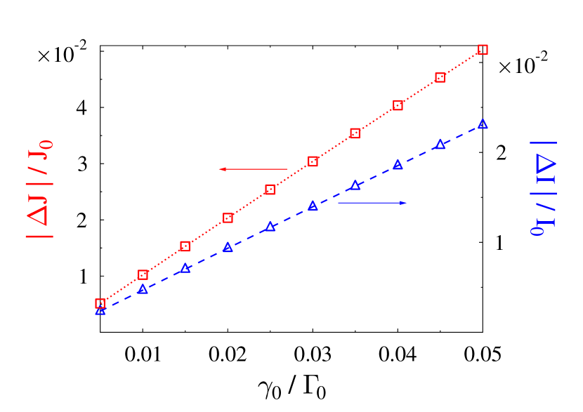
Figure 5: Violations of charge $\Delta I\equiv I_{L}+I_{R}$, Eq. (19) (triangles, dashed blue line), and energy $\Delta J\equiv J_{L}+J_{R}+J_{pt}$, Eq. (20) (squares, dotted red line), conservation laws from bare PT calculations as functions of the molecule-radiation field coupling strength $\gamma_{0}$ at $|e|V_{sd}=20E_{0}$.

Figure 4 shows results of the self-consistent (diagrammatic) and bare PT simulations. Optical flux coincides in the two approaches in the region of high positive biases, and differs in other regimes (see Fig. 4a). The effect is due to our choice of resonant optical transition between levels $2$ and $3$ of the molecule and the fact that for the choice of simulation parameters this transition defines the current through the junction at high biases. Indeed, Fig. 4b shows that current at the right interface calculated within the bare PT approach (dotted line, squares) coincides with the self-consistent diagrammatic result (solid line, circles) in the high bias region. However, charge conservation law, Eq. (19), is violated by the bare PT approach (compare dashed line, triangles and dotted line, squares). Also value of the charge flux is different between the two approaches at, e.g., negative biases. Similarly, energy conservation law, Eq. (20), is violated by the direct PT simulation (see Fig. 4c).

Figure 5 shows that (as expected) violation of the conservation laws in the bare PT simulation diminishes with the strength of molecular coupling to radiation field. We stress that the results are presented in the parameter range where diagrammatic perturbation treatment of molecular coupling to radiation field is applicable, $\gamma_{0}\ll\Gamma$. It is the improper version of the perturbation theory (the bare PT), which leads to inconsistencies in predictions of molecular junction responses.

Results of self-consistent calculation of optical spectrum of the junction is presented in Fig. 6 at the region of maximum discrepancy between the two approaches, $|e|V_{sd}=0$ (see Fig. 4a). Two peaks in the spectrum correspond to two electronic transitions in the model: $\varepsilon_{2}-\varepsilon_{1}$ and $\varepsilon_{2}-\varepsilon_{3}$. The spectrum scales with the strength of molecular coupling to the field (the latter correspond to intensity of the radiation), i.e. the junction operates near linear scaling of its optical response. However this seemingly linear behavior does not allow bare PT implementation as is demonstrated in Fig. 4.

Finally, we note that violations of conservation laws appear in the bare PT only for quantum radiation fields. Indeed, for classical fields (and within the rotating wave approximation) one always can formulate effective time-independent problem by transforming to the rotating frame of the field (see e.g. Ref. Peskin and Galperin (2012)). For the classical analog of the model (1)-(3) this transformation results in effective non-interacting model with fluxes defined by usual Landauer expressions. The latter are conserving by construction.

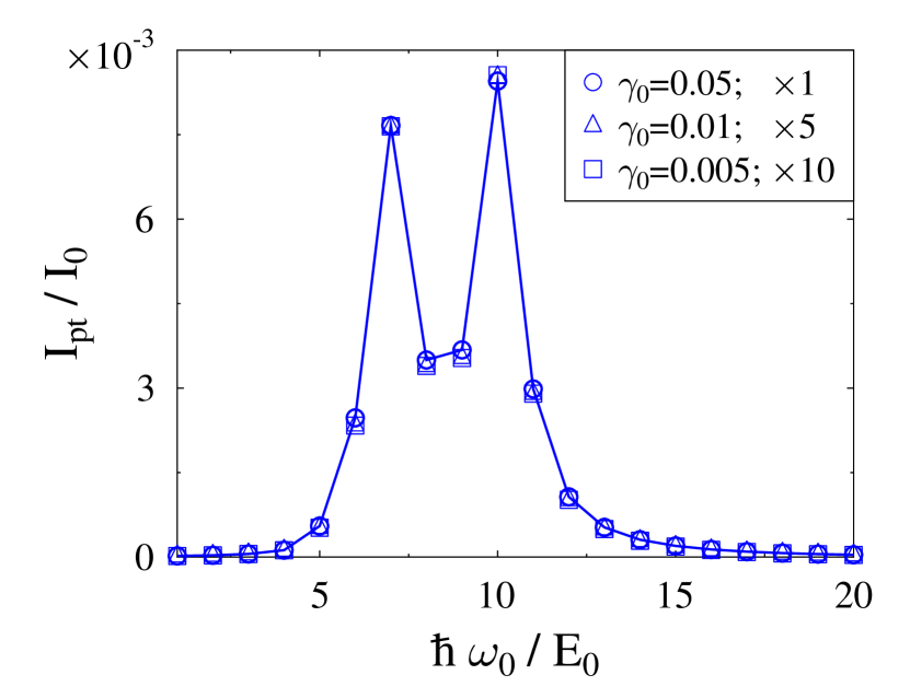
Figure 6: Optical spectrum of the junction for a number of molecule-field coupling strengths at $|e|V_{sd}=0$.

V Conclusions

We consider diagrammatic perturbation theory formulation for transport and optical spectroscopy of molecular junctions. Transport and optical response are characterized by electron and photon fluxes, respectively. Diagrammatic perturbation theory is known to impose a set of restrictions on the considered diagrams and involves resummation of infinite number of diagrams to assure conserving character of the resulting approximation Baym and Kadanoff (1961); Baym (1962). We then compare the formulation with the bare PT treatment of the molecule-field coupling, which is usually employed in the studies on nonlinear optical spectroscopy Mukamel (1995). We show that the finite order bare PT expansion violates the conserving character of the approximation. Results of model simulations within a reasonable parameter range demonstrate that the violation may be significant. We note that the self-consistent character of the diagrammatic perturbation approach (i.e. requirement of resummation of infinite number of diagrams) mixes elementary optical processes, which forbids utilization of the double-sided Feynman diagrams in molecular junctions (or for molecules chemisorbed on metal surfaces) when radiation field is treated quantum-mechanically.

We note that while our findings are illustrated with numerical examples employing simple junction model treated within fourth order perturbation in molecule-field coupling and at steady state, the conclusions are completely general. Indeed, requirement of self-consistency (resumming diagrams to infinite order) in constructing conserving approximations equally applicable to time-dependent processes, while any finite order subset is non-conserving Baym and Kadanoff (1961); Baym (1962). Moreover, presented analysis is equally applicable to quasiparticle (molecular orbital) Baym and Kadanoff (1961); Baym (1962); Luttinger and Ward (1960); De Dominicis and Martin (1964) or many-body states Eckstein and Werner (2010); Oh et al. (2011); Aoki et al. (2014) formulations.

Appendix A Derivation of fluxes expressions

Expression for electron current, Eq. (4) is a well known result (see, e.g., Ref. Haug and Jauho (2008)), so we will focus on derivation of the photon flux. We start from definition of the flux as rate of change of population in the bath (radiation field)

$$I_{pt}(t)\equiv\frac{d}{dt}\sum_{\alpha}\left\langle\hat{a}_{\alpha}^{\dagger}(t)\,\hat{a}_{\alpha}(t)\right\rangle=i\frac{d}{dt}\mbox{Tr}\left[F^{<}_{\alpha\alpha}(t,t)\right]$$ (35)

where

$$F^{<}_{\alpha_{1}\alpha_{2}}(t_{1},t_{2})=-i\left\langle\hat{a}_{\alpha_{2}}^{\dagger}(t_{2})\,\hat{a}_{\alpha_{1}}(t_{1})\right\rangle$$ (36)

is lesser projection of the photon Green function (7).

We then write differential forms of the Dyson equation, Eq. II, which for the lesser projection are

$$\bigg{(}i\frac{\partial}{\partial t_{1}}-\omega_{\alpha_{1}}\bigg{)}F_{\alpha_{1}\alpha_{2}}^{<}(t_{1},t_{2})=\int_{-\infty}^{+\infty}dt^{\prime}$$ (37)

$$\quad\bigg{(}\Pi_{\alpha_{1}\alpha^{\prime}}^{<}(t_{1},t^{\prime})\,F_{\alpha^{\prime}\alpha_{2}}^{a}(t^{\prime},t_{2})+\Pi_{\alpha_{1}\alpha^{\prime}}^{r}(t_{1},t^{\prime})\,F_{\alpha^{\prime}\alpha_{2}}^{<}(t^{\prime},t_{2})\bigg{)}$$

$$\bigg{(}-i\frac{\partial}{\partial t_{2}}-\omega_{\alpha_{2}}\bigg{)}F_{\alpha_{1}\alpha_{2}}^{<}(t_{1},t_{2})=\int_{-\infty}^{+\infty}dt^{\prime}$$ (38)

$$\quad\bigg{(}F_{\alpha_{1}\alpha^{\prime}}^{<}(t_{1},t^{\prime})\,\Pi_{\alpha^{\prime}\alpha_{2}}^{a}(t^{\prime},t_{2})+F_{\alpha_{1}\alpha^{\prime}}^{r}(t_{1},t^{\prime})\,\Pi_{\alpha^{\prime}\alpha_{2}}^{<}(t^{\prime},t_{2})\bigg{)}$$

Here superscripts $r$ and $a$ indicate retarded and advanced projections. Note that $F^{a}_{\alpha_{1}\alpha_{2}}(t_{1},t_{2})=[F^{r}_{\alpha_{2}\alpha_{1}}(t_{2},t_{1})]^{*}$ and $F^{<}_{\alpha_{1}\alpha_{2}}(t_{1},t_{2})=-[F^{<}_{\alpha_{2}\alpha_{1}}(t_{2},t_{1})]^{*}$ (and similar relations for projections of the self-energy $\Pi$).

Setting $\alpha_{1}=\alpha_{2}=\alpha$ and $t_{1}=t_{2}=t$, and utilizing (37) and (38) in (35) leads to

$$I_{pt}(t)=$$ (39)

$$2\,\mbox{Re}\int_{-\infty}^{+\infty}dt^{\prime}\,\mbox{Tr}\bigg{[}\Pi^{<}(t,t^{\prime})\,F^{a}(t^{\prime},t)+\Pi^{r}(t,t^{\prime})\,F^{<}(t^{\prime},t)\bigg{]}$$

Finally, using

$$F^{a}(t^{\prime},t)= \theta(t-t^{\prime})\big{[}F^{<}(t^{\prime},t)-F^{>}(t^{\prime},t)\big{]}$$ (40)

$$\Pi^{r}(t,t^{\prime})= \theta(t-t^{\prime})\big{[}\Pi^{>}(t,t^{\prime})-\Pi^{<}(t,t^{\prime})\big{]}$$ (41)

where $\theta(x)$ is the Heaviside step-function, leads to Eq. (5).

Appendix B Expressions for self-energies

Expressions for the self-energies (11) and (12) are derived following diagrammatic perturbation theory Mahan (1990); Fetter and Walecka (1971); Negele and Orland (1988), which for the model (1)-(3) leads to set of even in the interaction contributions

$$\Sigma^{pt}_{mm^{\prime}}(\tau,\tau^{\prime})= \sum_{n=1}^{\infty}\Sigma^{pt\,(2n)}_{mm^{\prime}}(\tau,\tau^{\prime})$$ (42)

$$\Pi_{\alpha\alpha^{\prime}}(\tau,\tau^{\prime})= \sum_{n=1}^{\infty}\Pi^{(2n)}_{\alpha\alpha^{\prime}}(\tau,\tau^{\prime})$$ (43)

Explicit expressions for second and fourth order are

$$\Sigma^{pt\,(2)}_{mm^{\prime}}(\tau,\tau^{\prime})= i\sum_{\alpha_{1},\alpha_{2}}\sum_{m_{1},m_{2}}G_{m_{1}m_{2}}(\tau,\tau^{\prime})\bigg{(}U_{m_{1}m,\alpha_{1}}F_{\alpha_{1},\alpha_{2}}(\tau,\tau^{\prime})U_{\alpha_{2},m_{2}m^{\prime}}+U_{m^{\prime}m_{2},\alpha_{2}}F_{\alpha_{2}\alpha_{1}}(\tau^{\prime},\tau)U_{\alpha_{1},mm_{1}}\bigg{)}$$ (44)

$$\Sigma^{pt\,(4)}_{mm^{\prime}}(\tau,\tau^{\prime})= -\sum_{\begin{subarray}{c}\alpha_{1},\alpha_{2}\\ \alpha_{3},\alpha_{4}\end{subarray}}\sum_{\begin{subarray}{c}m_{1},m_{2},m_{3}\\ m_{4},m_{5},m_{6}\end{subarray}}\int_{c}d\tau_{1}\int_{c}d\tau_{2}\,G_{m_{1}m_{2}}(\tau,\tau_{1})\,G_{m_{3}m_{4}}(\tau_{1},\tau_{2})\,G_{m_{5}m_{6}}(\tau_{2},\tau^{\prime})$$

$$\times\bigg{(}U_{M_{1}m,\alpha_{1}}F_{\alpha_{1}\alpha_{4}}(\tau,\tau_{2})U_{\alpha_{4},m_{4}m_{5}}+U_{m_{5}m_{4},\alpha_{4}}F_{\alpha_{4}\alpha_{1}}(\tau_{2},\tau)U_{\alpha_{1},mm_{1}}\bigg{)}$$ (45)

$$\times\bigg{(}U_{m^{\prime}m_{6},\alpha_{2}}F_{\alpha_{2}\alpha_{3}}(\tau^{\prime},\tau_{1})U_{\alpha_{3},m_{2}m_{3}}+U_{m_{3}m_{2},\alpha_{3}}F_{\alpha_{3}\alpha_{2}}(\tau_{1},\tau^{\prime})U_{\alpha_{2},m_{6}m^{\prime}}\bigg{)}$$

for the electron self-energy, and

$$\Pi^{(2)}_{\alpha\alpha^{\prime}}(\tau,\tau^{\prime})=-i\sum_{\begin{subarray}{c}m_{1},m_{2}\\ m_{3},m_{4}\end{subarray}}U_{\alpha,m_{1}m_{2}}\,G_{m_{2}m_{4}}(\tau,\tau^{\prime})\,G_{m_{3}m_{1}}(\tau^{\prime},\tau)\,U_{m_{3}m_{4},\alpha_{2}}$$ (46)

$$\Pi^{(4)}_{\alpha\alpha^{\prime}}(\tau,\tau^{\prime})=\sum_{\alpha_{1},\alpha_{2}}\sum_{\begin{subarray}{c}m_{1},m_{2},m_{3},m_{4}\\ m_{5},m_{6},m_{7},m_{8}\end{subarray}}\int_{c}d\tau_{1}\int_{c}d\tau_{2}\,U_{\alpha,m_{1}m_{2}}U_{m_{3}m_{4},\alpha_{1}}F_{\alpha_{1}\alpha_{2}}(\tau_{1},\tau_{2})U_{\alpha_{2},m_{7}m_{8}}U_{m_{5}m_{6},\alpha^{\prime}}$$ (47)

$$\times\bigg{(}G_{m_{2}m_{4}}(\tau,\tau_{1})\,G_{m_{3}m_{6}}(\tau_{1},\tau^{\prime})\,G_{m_{5}m_{7}}(\tau^{\prime},\tau_{2})\,G_{m_{8}m_{1}}(\tau_{2},\tau)+G_{m_{2}m_{7}}(\tau,\tau_{2})\,G_{m_{8}m_{5}}(\tau_{2},\tau^{\prime})\,G_{m_{5}m_{4}}(\tau^{\prime},\tau_{1})\,G_{m_{3}m_{1}}(\tau_{1},\tau)\bigg{)}$$

for the photon self-energy.

References

- Wu et al. (2008) S. W. Wu, G. V. Nazin, and W. Ho, Phys. Rev. B 77, 205430 (2008).
- Ioffe et al. (2008) Z. Ioffe, T. Shamai, A. Ophir, G. Noy, I. Yutsis, K. Kfir, O. Cheshnovsky, and Y. Selzer, Nature Nanotech. 3, 727 (2008).
- Ward et al. (2008) D. R. Ward, N. J. Halas, J. W. Ciszek, J. M. Tour, Y. Wu, P. Nordlander, and D. Natelson, Nano Lett. 8, 919 (2008).
- Ward et al. (2011) D. R. Ward, D. A. Corley, J. M. Tour, and D. Natelson, Nature Nanotech. 6, 33 (2011).
- Chen et al. (2010) C. Chen, P. Chu, C. A. Bobisch, D. L. Mills, and W. Ho, Phys. Rev. Lett. 105, 217402 (2010).
- Schneider et al. (2012) N. L. Schneider, J. T. Lü, M. Brandbyge, and R. Berndt, Phys. Rev. Lett. 109, 186601 (2012).
- Grosse et al. (2013) C. Grosse, M. Etzkorn, K. Kuhnke, S. Loth, and K. Kern, Appl. Phys. Lett. 103, 183108 (2013).
- Selzer and Peskin (2013) Y. Selzer and U. Peskin, J. Phys. Chem. C 117, 22369 (2013).
- Ochoa et al. (2015) M. A. Ochoa, Y. Selzer, U. Peskin, and M. Galperin, J. Phys. Chem. Lett. 6, 470 (2015).
- Galperin and Nitzan (2012) M. Galperin and A. Nitzan, Phys. Chem. Chem. Phys. 14, 9421 (2012).
- Mukamel (1995) S. Mukamel, Principles of Nonlinear Optical Spectroscopy (Oxford University Press, 1995).
- Okumura and Tanimura (1997a) K. Okumura and Y. Tanimura, J. Chem. Phys. 106, 1687 (1997a).
- Okumura and Tanimura (1997b) K. Okumura and Y. Tanimura, J. Chem. Phys. 107, 2267 (1997b).
- Xu et al. (2001) Q.-H. Xu, , and G. R. Fleming, J. Phys. Chem. A 105, 10187 (2001).
- Ovchinnikov et al. (2001) M. Ovchinnikov, V. A. Apkarian, and G. A. Voth, J. Chem. Phys. 114, 7130 (2001).
- Okumura and Tanimura (2003) K. Okumura and Y. Tanimura, J. Phys. Chem. A 107, 8092 (2003).
- Mukamel et al. (2004) S. Mukamel, , and D. Abramavicius, Chem. Rev. 104, 2073 (2004).
- Šanda and Mukamel (2005) F. Šanda and S. Mukamel, Phys. Rev. A 71, 033807 (2005).
- Yang and Mukamel (2008) L. Yang and S. Mukamel, Phys. Rev. B 77, 075335 (2008).
- Harbola and Mukamel (2009) U. Harbola and S. Mukamel, Phys. Rev. B 79, 085108 (2009).
- Harbola et al. (2006) U. Harbola, J. B. Maddox, and S. Mukamel, Phys. Rev. B 73, 075211 (2006).
- Harbola et al. (2014) U. Harbola, B. K. Agarwalla, and S. Mukamel, J. Chem. Phys. 141, 074107 (2014).
- Goswami et al. (2015) H. P. Goswami, W. Hua, Y. Zhang, S. Mukamel, and U. Harbola, J. Chem. Theory Comput. 11, 4304 (2015).
- Agarwalla et al. (2015) B. K. Agarwalla, U. Harbola, W. Hua, Y. Zhang, and S. Mukamel, J. Chem. Phys. 142, 212445 (2015).
- Rahav and Mukamel (2010) S. Rahav and S. Mukamel, Proc. Natl. Acad. Sci. 107, 4825 (2010).
- Mukamel and Rahav (2010) S. Mukamel and S. Rahav, in Advances in Atomic, Molecular, and Optical Physics, Advances In Atomic, Molecular, and Optical Physics, Vol. 59, edited by P. B. E. Arimondo and C. Lin (Academic Press, 2010) pp. 223 – 263.
- Lodahl et al. (2015) P. Lodahl, S. Mahmoodian, and S. Stobbe, Rev. Mod. Phys. 87, 347 (2015).
- Galperin et al. (2009a) M. Galperin, M. A. Ratner, and A. Nitzan, Nano Lett. 9, 758 (2009a).
- Galperin et al. (2009b) M. Galperin, M. A. Ratner, and A. Nitzan, J. Chem. Phys. 130, 144109 (2009b).
- Park and Galperin (2011a) T.-H. Park and M. Galperin, Europhys. Lett. 95, 27001 (2011a).
- Park and Galperin (2011b) T.-H. Park and M. Galperin, Phys. Rev. B 84, 075447 (2011b).
- Galperin and Nitzan (2011a) M. Galperin and A. Nitzan, J. Phys. Chem. Lett. 2, 2110 (2011a).
- Galperin and Nitzan (2011b) M. Galperin and A. Nitzan, Phys. Rev. B 84, 195325 (2011b).
- Oren et al. (2012) M. Oren, M. Galperin, and A. Nitzan, Phys. Rev. B 85, 115435 (2012).
- Banik et al. (2013) M. Banik, V. A. Apkarian, T.-H. Park, and M. Galperin, J. Phys. Chem. Lett. 4, 88 (2013).
- White et al. (2014) A. J. White, S. Tretiak, and M. Galperin, Nano Lett. 14, 699 (2014).
- Galperin et al. (2015) M. Galperin, M. A. Ratner, and A. Nitzan, J. Chem. Phys. 142, 137101 (2015).
- Dey et al. (2016) S. Dey, M. Banik, E. Hulkko, K. Rodriguez, V. A. Apkarian, M. Galperin, and A. Nitzan, Phys. Rev. B 93, 035411 (2016).
- Sukharev and Galperin (2010) M. Sukharev and M. Galperin, Phys. Rev. B 81, 165307 (2010).
- Kinoshita et al. (1995) I. Kinoshita, A. Misu, and T. Munakata, J. Chem. Phys. 102, 2970 (1995).
- Stefanucci and van Leeuwen (2013) G. Stefanucci and R. van Leeuwen, Nonequilibrium Many-Body Theory of Quantum Systems. A Modern Introduction. (Cambridge University Press, 2013).
- Baym and Kadanoff (1961) G. Baym and L. P. Kadanoff, Phys. Rev. 124, 287 (1961).
- Baym (1962) G. Baym, Phys. Rev. 127, 1391 (1962).
- Galperin and Nitzan (2005) M. Galperin and A. Nitzan, Phys. Rev. Lett. 95, 206802 (2005).
- Galperin and Nitzan (2006) M. Galperin and A. Nitzan, J. Chem. Phys. 124, 234709 (2006).
- Haug and Jauho (2008) H. Haug and A.-P. Jauho, Quantum Kinetics in Transport and Optics of Semiconductors (Springer, Berlin Heidelberg, 2008).
- Galperin et al. (2007) M. Galperin, A. Nitzan, and M. A. Ratner, Phys. Rev. B 75, 155312 (2007).
- Luttinger and Ward (1960) J. M. Luttinger and J. C. Ward, Phys. Rev. 118, 1417 (1960).
- De Dominicis and Martin (1964) C. De Dominicis and P. C. Martin, J. Math. Phys. 5, 14 (1964).
- Haussmann (1999) R. Haussmann, Self-consistent Quantum-Field Theory and Bosonization for Strongly Correlated Electron Systems (Springer-Verlag, Berlin Heidelberg, 1999).
- White and Galperin (2012) A. J. White and M. Galperin, Phys. Chem. Chem. Phys. 14, 13809 (2012).
- Fetter and Walecka (1971) A. L. Fetter and J. D. Walecka, Quantum Theory of Many-Particle Systems (McGraw-Hill Book Company, 1971).
- Mahan (1990) G. D. Mahan, Many-Particle Physics (Plenum Press, 1990).
- Wagner (1991) M. Wagner, Phys. Rev. B 44, 6104 (1991).
- Caroli et al. (1972) C. Caroli, R. Combescot, P. Nozieres, and D. Saint-James, J. Phys. C 5, 21 (1972).
- White et al. (2012) A. J. White, B. D. Fainberg, and M. Galperin, J. Phys. Chem. Lett. 3, 2738 (2012).
- Ponder and Mathies (1983) M. Ponder and R. Mathies, J. Phys. Chem. 87, 5090 (1983).
- Colvin and Alivisatos (1992) V. L. Colvin and A. P. Alivisatos, J. Chem. Phys. 97, 730 (1992).
- Nie and Emory (1997) S. Nie and S. R. Emory, Science 275, 1102 (1997).
- Peskin and Galperin (2012) U. Peskin and M. Galperin, J. Chem. Phys. 136, 044107 (2012).
- Eckstein and Werner (2010) M. Eckstein and P. Werner, Phys. Rev. B 82, 115115 (2010).
- Oh et al. (2011) J. H. Oh, D. Ahn, and V. Bubanja, Phys. Rev. B 83, 205302 (2011).
- Aoki et al. (2014) H. Aoki, N. Tsuji, M. Eckstein, M. Kollar, T. Oka, and P. Werner, Rev. Mod. Phys. 86, 779 (2014).
- Negele and Orland (1988) J. W. Negele and H. Orland, Quantum Many-Particle Systems, edited by D. Pines (Addison-Wesley Publishing Company, Redwood City, California, 1988).