Cooperative quantum electrodynamical processes in an ellipsoidal cavity

Abstract

We investigate spontaneous photon emission and absorption processes of two two-level atoms trapped close to the focal points of an ellipsoidal cavity, thereby taking into account the full multimode scenario. In particular, we calculate the excitation probabilities of the atoms by describing the field modes semiclassically. Based on this approach, we express the excitation probabilities by a semiclassical photon path representation. Due to the special property of an ellipsoidal cavity of having two focal points, we are able to study interesting intermediate instances between well-known quantum-optical scenarios. Furthermore, the semiclassical photon path representation enables us to address the corresponding retardation effects and causality questions in a straightforward manner.

1 Introduction

During the last decades, the field of quantum optics has witnessed remarkable experimental developments. They have enabled new possibilities of studying resonant light-matter interaction [1, 2, 3]. These developments are not only interesting from a fundamental point of view, but also from an applied perspective, because they are relevant for advanced quantum technologies and their possible application in quantum information processing.

Understanding light-matter interaction is crucial for being able to transfer quantum information between single photons, frequently used as flying qubits, and elementary material systems, typically used as stationary qubits in applications in quantum information. Such a transfer of quantum information between single photons and elementary material systems, such as two level systems serving as qubits, is an integral building block for achieving quantum communication over large distances. Recently, considerable experimental effort [4, 5, 6] has been devoted to investigating the interaction of matter qubits with one or a few selected modes of the radiation field within the framework of the Jaynes-Cummings-Paul model [7, 8]. Recent experimental work has extended these quantum electrodynamical scenarios to the opposite limit of extreme multimode scenarios [9, 10, 11] with structured continua of electromagnetic field modes characteristic for half open cavities, such as a parabolic mirror[12, 13, 14].

Motivated by these latter developments, we explore in this paper basic dynamical features of quantum electrodynamic processes in extreme multimode scenarios. In particular, we investigate the almost resonant interaction between two two-level systems located at the focal points of a prolate-ellipsoidal cavity and the quantized electromagnetic field. A particularly interesting elementary quantum electrodynamical situation arises if these two atoms exchange a single photon emitted spontaneously by one of these two-level systems. Due to the special property of the prolate-ellipsoidal cavity of having two focal points, the electromagnetic field strength around the focal points is enhanced significantly, thus causing an interesting interaction between the two-level systems and the radiation field. From the point of view of the two-level systems as an open quantum system, the resulting reduced dynamics is highly non-Markovian with significant memory effects. Thus, an ellipsoidal cavity is an interesting scenario to study almost resonant matter field interaction. In particular, by changing the size of the cavity continuously, all intermediate cases between the single mode scenario, as described by the Jaynes-Cummings-Paul model, the large cavity limit, and the case of a structured continua of field modes can be addressed. Even the recently explored case of a parabolic cavity [15] can be reproduced in the limit of infinitely separated focal points. Furthermore, we are able to tune the coupling strength between the two-level systems and the radiation field by changing the shape of the cavity. In addition, we are able to investigate diffraction effects in the regime of wavelengths large in comparison to the characteristic length scales inside the cavity and their extinction in the geometric optical limit of small wavelengths. In the following it is demonstrated that all these effects can be described adequately with the help of a semiclassical description of the mode structure inside the ellipsoidal cavity. We show that these semiclassical methods lead to a convenient photon path representation by which all relevant quantum mechanical transition amplitudes are expressed as a linear superposition of contributions of relevant photon paths inside the cavity.

This paper is organized as follows. In Sec. 2 we introduce our theoretical model and the main approximations involved. The Helmholtz equation with the appropriate boundary conditions is solved by semiclassical methods in Sec. 3. The photon path representation for describing the time evolution of relevant quantum mechanical transition amplitudes is presented in Sec. 4. Numerical results for the dynamics of the two-level systems are discussed in Sec. 5.

2 Quantum electrodynamical model

We investigate the dynamics of two identical two-level systems, e.g. atoms or ions, situated at the focal points $\mathbf{x}_{a}$ ($a\in\left\{1,2\right\}$) of an ideally conducting prolate-ellipsoidal cavity as shown schematically in Fig. 1. Both atoms interact with the quantized radiation field inside this cavity. The two two-level systems are assumed to be trapped in such a way that their center of mass motion is negligible. We assume that the dipole matrix elements $\mathbf{d}_{a}=\bra{e}_{a}\hat{\mathbf{d}}_{a}\ket{g}_{a}$ are oriented along the symmetry axis, i.e. $z-$axis, of the system so that we may write

$$\mathbf{d}_{a}=D\mathbf{e}_{z}\;\text{with }D\in\mathbb{R}.$$ (1)

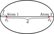
Figure 1: Two two-level systems located in the foci of a prolate-ellipsoidal cavity.

The identical transition frequencies $\omega_{eg}$ of the two-level systems are assumed to be in the optical frequency regime and to dominate the coupling to the radiation field as measured by relevant Rabi frequencies, for example. Furthermore, the sizes of the electronic states involved in the transitions of the two-level systems are supposed to be small compared to the corresponding wavelength $\lambda_{\text{eg}}=2\pi c_{0}/\omega_{eg}$ of the transition. ($c_{0}$ being the speed of light in vacuum.) Thus, the dipole and the rotating-wave approximation (RWA) are applicable. Therefore, the quantum electrodynamical interaction between the two two-level systems and the quantized electromagnetic field inside the cavity is described by the Hamiltonian

$$\hat{H}=\hat{H}_{\text{atoms}}+\hat{H}_{\text{field}}+\hat{H}_{\text{i}}$$ (2)

with $\hat{H}_{\text{field}}=\sum_{i}\hbar\omega_{i}\hat{a}_{i}^{\dagger}\hat{a}_{i}$, $\hat{H}_{\text{atoms}}=\hbar\omega_{eg}\sum\limits_{a=1}^{2}\ket{e}_{a}\bra{e}_{a},$ $\hat{H}_{\text{i}}=-\sum\limits_{a=1}^{2}\hat{\mathbf{E}}_{\perp}^{+}(\mathbf{x}_{a})\cdot\hat{\mathbf{d}}_{a}^{-}+\text{H.c.}$, and with the dipole transition operator $\hat{\mathbf{d}}_{a}^{-}=\mathbf{d}_{a}^{*}\ket{g}_{a}\bra{e}_{a}$ of the two-level atom $a\in\left\{1,2\right\}$. In the Schrödinger picture the positive frequency part of the (transversal) electromagnetic field operator is given by

$$\hat{\mathbf{E}}_{\perp}^{+}(\mathbf{x})=-\mathrm{i}\sum_{i}\sqrt{\frac{\hbar\omega_{i}}{2\epsilon_{0}}}\mathbf{g}_{i}(\mathbf{x})\hat{a}_{i}^{\dagger}$$ (3)

with $\mathbf{g}_{i}(\mathbf{x})$ denoting the orthonormal transversal electric mode functions, i.e. $\int_{V}d^{3}{\bf x}~{}\mathbf{g}_{i}^{*}(\mathbf{x})\cdot\mathbf{g}_{j}(\mathbf{x})=\delta_{ij}$, which are assumed to fulfill the boundary conditions for an ideally conducting cavity.

3 Mode functions of the cavity and their semiclassical approximation

3.1 Separation ansatz for the relevant mode functions

In order to determine the electric mode functions by solving the Helmholtz equation, we are going to use prolate-ellipsoidal coordinates. The connection between the prolate-ellipsoidal coordinates and the Cartesian coordinates is given by

$$\left(\begin{array}[]{c}x\\ y\\ z\end{array}\right)=\frac{d}{2}\left(\begin{array}[]{c}\cos(\varphi)\sqrt{(1-\eta^{2})(\xi^{2}-1)}\\ \sin(\varphi)\sqrt{(1-\eta^{2})(\xi^{2}-1)}\\ \eta\xi\end{array}\right).$$ (4)

Thereby, the focal points have been chosen to be located at the positions $\pm\mathbf{e}_{z}d/2$ and $d$ denotes their distance. The ranges of the prolate-ellipsoidal coordinates are given by $\varphi\in[0,2\pi)$, $\eta\in[-1,1]$, and $\xi\in[1,\infty)$. In particular, the focal points have the coordinates $\xi=1$, $\eta=\pm 1$. In these new coordinates an ellipsoid with the focal length $f$ is defined by the surface

$$\xi=2f/d+1\;.$$ (5)

Only those mode functions enter the interaction Hamiltonian $\hat{H}_{\text{i}}$ which have a nonvanishing scalar product with the dipole transition operators of the two two-level systems situated in the focal points of the cavity. By taking into account the transversality of the radiation field, it turns out that for dipole matrix elements oriented along the $z$-axis all these modes can be obtained by a separation ansatz. This separation ansatz is given by

$$\mathbf{g}_{i}(\varphi,\xi,\eta)=\nabla\times H,\;H=\frac{1}{\mathcal{N}}\mathbf{e}_{\varphi}\mathcal{F}_{i}(\kappa,\xi)\mathcal{G}_{i}(\kappa,\eta)\;,$$ (6)

with

$$\left[\alpha_{n}\kappa-\kappa^{2}\left(\eta^{2}-1\right)-\frac{1}{1-\eta^{2}}\right]\mathcal{G}(\kappa,\eta)+\frac{d}{d\eta}(1-\eta^{2})\frac{d}{d\eta}\mathcal{G}(\kappa,\eta) = 0\;,$$

$$\left[\alpha_{n}\kappa-\kappa^{2}\left(\xi^{2}-1\right)-\frac{1}{1-\xi^{2}}\right]\mathcal{F}(\kappa,\xi)+\frac{d}{d\xi}(1-\xi^{2})\frac{d}{d\xi}\mathcal{F}(\kappa,\xi) = 0\;,$$

whereby $\kappa=\omega d/(2c_{0})$ , $\alpha_{n}$ being the constant of separation and $\mathcal{N}$ being the normalization factor which has to be chosen such that

$$\int\limits_{V}\mathbf{g}_{i}(x)\cdot\mathbf{g}_{j}^{*}(x)d^{3}x=\delta_{i,j}\;\forall i,j\;.$$ (9)

The index $n$ indicates that $\mathcal{G}(\kappa,\eta)$ remains finite for $\eta\rightarrow\pm 1$ only for countable sets of the separation constant $\alpha_{n}$. The differential equations Eq. (LABEL:eq:DGL_S_eta) and Eq. (LABEL:eq:DGL_R_xi) are actually identical, and the functions $\mathcal{G}$ and $\mathcal{F}$ just differ by the domains for $\eta$ and $\xi$. The solutions of these differential equations are prolate-spheroidal wave functions [16].

3.2 Uniform semiclassical approximation

In the previous section, we have expressed the mode functions of the electric field operator in terms of prolate-spheroidal wave functions. We can obtain an analytical solution for this equations in the special case of $\alpha_{n}=0$

$$\mathcal{G}(\kappa,\eta)\Bigr{|}_{\alpha_{n}=0} = \frac{\text{sin}[\kappa(1-\eta)]}{\sqrt{1-\eta^{2}}},$$ (10)

$$\mathcal{F}(\kappa,\xi)\Bigr{|}_{\alpha_{n}=0} = \frac{\text{sin}[\kappa(\xi-1)]}{\sqrt{\xi^{2}-1}}\;.$$ (11)

A general closed analytical expression for arbitrary values is not known. However, with the help of semiclassical methods, approximate expressions can be found. It turns out that the mode functions with $\alpha_{n}\approx 0$ yield the dominant contributions. Therefore, we can exploit the exact analytical solutions for $\alpha_{n}=0$ in order to improve our approximation. It is convenient to choose the following normalization conditions for the functions $\mathcal{F}(\kappa,\xi)$ and $\mathcal{G}(\kappa,\eta)$

$$\mathcal{F}(\kappa,\xi) \underset{\kappa\xi\rightarrow\infty}{\longrightarrow} \frac{1}{\xi}\cos\left[\kappa\xi-\frac{1}{2}\left(n+1\right)\pi\right],$$

$$\mathcal{G}(\kappa,0) = (-1)^{(n+1)/2}\;\text{in case of odd }n,$$

$$\frac{d}{d\eta}\mathcal{G}(\kappa,\eta)\Bigr{|}_{\eta=0} = (-1)^{n/2}\kappa\;\text{in case of even }n.$$

These conditions are fulfilled by the exact solutions in Eq. (10) and Eq. (11).

In order to circumvent problems originating from the singularities of the differential equations (LABEL:eq:DGL_S_eta) and (LABEL:eq:DGL_R_xi), we first of all apply a transformation which removes these singularities at the positions of the focal points. Let us demonstrate this procedure by concentrating on the functions $\mathcal{F}(\kappa,\xi)$. The procedure for the functions $\mathcal{G}(\kappa,\eta)$ is analogous because the differential equations for $\mathcal{F}$ and for $\mathcal{G}$ coincide. A transformation removing the singularities is given by

$$\mathcal{F}(\kappa,\xi)=\frac{1}{\sqrt{\xi^{2}-1}}f(\sqrt{\xi^{2}-1})\;.$$ (13)

Consequently, the function $f(x)$ with $x\in[0,\infty)$ is a solution of the differential equation

$$0=\kappa^{2}x\left(x^{2}-\frac{\alpha_{n}}{\kappa}\right)f(x)-f^{\prime}(x)+x\left(1+x^{2}\right)f^{\prime\prime}(x)$$ (14)

with $x=\sqrt{\xi^{2}-1}$. The focal points correspond to $x=0$. For the determination of the relevant mode functions, we are only interested in the regular (physical) solution of Eq. (14) which remains finite for all possible values of $x\geq 0$.

A uniform semiclassical JWKB-approximation [17] for the solution of Eq. (14) can be constructed by using the differential equation

$$\kappa^{2}\sigma\left(\sigma^{2}-\frac{\alpha_{n}}{\kappa}\right)\tilde{f}(\sigma)-\tilde{f}^{\prime}(\sigma)+\sigma\tilde{f}^{\prime\prime}(\sigma)=0\;,$$ (15)

as a comparison equation with the exact regular solution

$$\tilde{f}(\sigma)=e^{-\mathrm{i}\kappa\sigma^{2}/2}\kappa\sigma^{2}\,_{1}F_{1}\left(1-\mathrm{i}\alpha_{n}/4;2;i\kappa\sigma^{2}\right)\;.$$ (16)

In Eq. (16) ${}_{1}F_{1}$ denotes Kummer’s confluent hypergeometric function [18]. Accordingly, we are going to solve Eq. (14) by constructing a sufficiently smooth mapping between the variables $x$ and $\sigma$ in such a way that fulfillment of Eq. (14) is approximately equivalent to fulfillment of Eq. (15). For this purpose, we transform Eq. (14) into a canonical form by eliminating the terms involving first order derivates. This is achieved by the transformation $f(x)=\phi(x)u(x)$ with

$$\phi(x)=\frac{\sqrt{x}}{\left(1+x^{2}\right)^{1/4}}.$$ (17)

The resulting canonical form of Eq. (14) is given by

$$u^{\prime\prime}(x)+\chi(x)u(x) = 0$$ (18)

with

$$\chi(x)=\frac{2x^{2}\left(2\kappa\left(x^{2}+1\right)\left(\kappa x^{2}-\alpha_{n}\right)-3\right)-3}{4\left(x^{3}+x\right)^{2}}\;.$$ (19)

In order to find a uniform JWKB-approximation for Eq. (18), we have to chose an appropriate comparison equation whose solution is known exactly. For our purposes, we chose the comparison equation

$$\tilde{u}^{\prime\prime}(\sigma)+\Pi(\sigma)\tilde{u}(\sigma) = 0$$ (20)

with

$$\Pi(\sigma)=\kappa^{2}\sigma^{2}-\alpha_{n}\kappa-\frac{3}{4\sigma^{2}}.$$ (21)

This comparison equation is related to the differential equation (15) by the relation $\tilde{f}(\sigma)=\sqrt{\sigma}\tilde{u}(\sigma)$. Furthermore, we have to choose a smooth mapping between the independent variables $x$ and $\sigma$ determined by the relation

$$\frac{d\sigma}{dx} = \sqrt{\frac{\chi(x)}{\Pi(\sigma(x))}}\;.$$ (22)

The initial condition for the solution of Eq. (22) has to be chosen such that the first positive zero of $\chi(x)$, i.e. $x_{0}$, is mapped onto the first positive zero of $\Pi(\sigma)$, i.e. $\sigma_{0}$, in order to avoid singularities. Solving Eq. (22) analytically is a complicated problem. However, simple expressions are available for $x\rightarrow 0$ and $x\rightarrow\infty$ which are given by $\sigma(x)\underset{x\rightarrow 0}{\longrightarrow}x$ and $\sigma(x)\underset{x\rightarrow\infty}{\longrightarrow}\sqrt{2x}$. The behavior for $x\rightarrow 0$ is of importance in order to evaluate the mode function near the focal points and $x\rightarrow\infty$ is relevant for the normalization (Eq. (LABEL:normalization)). Thus, the JWKB-approximation for $\mathcal{F}(\kappa,\xi)$ is finally given by

$$\mathcal{F}(\kappa,\xi)=\frac{1}{\left(\xi^{2}\left(-1+\xi^{2}\right)\right)^{1/4}}{\left(\frac{\Pi(\sigma(\sqrt{\xi^{2}-1}))}{\chi(\sqrt{\xi^{2}-1})}\right)}^{1/4}\psi(\sigma(\sqrt{\xi^{2}-1}))$$

with [18]

$$\psi(\sigma)=e^{-\pi\alpha_{n}/8}\text{ }\sqrt{\frac{\pi\alpha_{n}}{16\sigma}\text{csch}\left(\frac{\pi\alpha_{n}}{4}\right)}\tilde{f}(\sigma).$$ (24)

This expression for $\mathcal{F}(\kappa,\xi)$ fulfills the normalization condition Eq. (LABEL:normalization). The normalized mode function at the first focal point is now given by

$$\mathbf{g}_{i}(\varphi,\xi,\eta)\Bigr{|}_{\eta=1,\xi=1}=$$

$$\mathbf{e}_{z}\frac{4}{d\mathcal{N}(\kappa,\alpha_{n})}\left(\lim\limits_{\xi\rightarrow 1}\frac{\mathcal{F}(\kappa,\xi)}{\sqrt{\xi^{2}-1}}\right)\left(\lim\limits_{\eta\rightarrow 1}\frac{\mathcal{G}(\kappa,\eta)}{\sqrt{1-\eta^{2}}}\right)$$

$$=\mathbf{e}_{z}\frac{\kappa^{2}\pi}{4d\mathcal{N}(\kappa,\alpha_{n})}\alpha_{n}\text{csch}\left({\pi\alpha_{n}}/{4}\right)\;.$$ (25)

By exploiting the symmetry of the problem, we can evaluate the mode function at the second focal point and obtain

$$\mathbf{g}_{i}(\varphi,\xi,\eta)\Bigr{|}_{\eta=-1,\xi=1}=(-1)^{n}\mathbf{g}_{i}(\varphi,\xi,\eta)\Bigr{|}_{\eta=1,\xi=1}\;.$$ (26)

In order to normalize the mode functions according to Eq. (9) we have to determine the constant $\mathcal{N}(\kappa,\alpha_{n})$, i.e.

$$\mathcal{N}(\kappa,\alpha_{n})=\kappa\sqrt{d\pi(I_{\mathcal{F}}^{2}I_{\mathcal{G}}^{0}-I_{\mathcal{F}}^{0}I_{\mathcal{G}}^{2})}$$ (27)

with ($p=0,2$)

$$I_{\mathcal{G}}^{p}=2\int\limits_{0}^{1}\mathcal{G}(\kappa,\eta)^{2}\eta^{p}d\eta\text{ and }I_{\mathcal{F}}^{p}=\int\limits_{1}^{1+2f/d}\mathcal{F}(\kappa,\xi)^{2}\xi^{p}d\xi.$$

According to Eqs. (25) and (26) at the focal points the normalized mode functions are determined by the function $\mathcal{N}(\kappa,\alpha_{n})$ and the function $\alpha_{n}\text{csch}\left(\pi\alpha_{n}/4\right)$. The function $\alpha_{n}\text{csch}\left(\pi\alpha_{n}/4\right)$ significantly deviates from 0 only in the region around $\alpha_{n}=0$. It turns out that in this region $\mathcal{N}(\kappa,\alpha_{n})$ is slowly varying in comparison with the function $\alpha_{n}\text{csch}\left(\pi\alpha_{n}/4\right)$ in case of $\lambda_{eg}\ll d,f$. This can be verified by using the semiclassical potential $\chi(x)$ and a corresponding potential for the semiclassical treatment of $\mathcal{G}$. Thus the modes with $\alpha_{n}\approx 0$ are the ones of main importance as far as their coupling to the dipoles of the two-level systems is concerned and $\mathcal{N}(\kappa,\alpha_{n})$ can be assumed to be independent of $\alpha_{n}$. In addition it is also well-known that the relevant modes have the property $\omega\approx\omega_{eg}$ which directly translates to $\kappa\approx\kappa_{eg}=2\omega_{eg}d/c_{0}$ . By incorporating these facts we can approximate $\mathcal{N}(\kappa,\alpha_{n})$ by $\mathcal{N}(\kappa_{eg},0)$ in the subsequent calculation.

3.3 Semiclassical quantization functions

In the previous subsection, we have identified the modes in the region of $\alpha_{n}\approx 0$, $\kappa\approx\kappa_{eg}$ as the ones of main importance for the dynamics of the system. However, in the case of $\alpha_{n}=0$ , Eqs. (LABEL:eq:DGL_S_eta) and (LABEL:eq:DGL_R_xi) can be solved analytically. This particular feature of the mode functions can be exploited for incorporating the boundary conditions of an ideally conducting metallic boundary and determining the corresponding quantization functions semiclassically. These quantization functions $n_{1}(\alpha_{n},\kappa),$ and $n_{2}(\alpha_{n},\kappa)$ are defined in such a way that the condition

$$\left(n_{1}(\alpha_{n},\kappa),n_{2}(\alpha_{n},\kappa)\right)\in\mathbb{N}_{0}\times\mathbb{N}_{0}$$ (29)

determines the possible mode functions which fulfill the boundary conditions.

The quantization function $n_{1}(\alpha_{n},\kappa)$ is determined by imposing the condition that the function $\mathcal{G}(\kappa,\eta)$ has to remain finite for $\eta\rightarrow\pm 1$. The quantization function $n_{2}(\alpha_{n},\kappa)$ takes into account the boundary conditions of an ideally conducting surface of the cavity. In particular, this implies that the tangential components of the electric field strength and the normal components of the magnetic field strength have to vanish at the boundary which yield the constraint

$$0=\frac{\partial}{\partial\xi}\left[\sqrt{\xi^{2}-1}\mathcal{F}(\kappa,\xi)\right]{}_{\xi={2f}/{d}+1}\;.$$ (30)

As mentioned above we have to evaluate the quantization functions around $\alpha_{n}\approx 0$ and $\kappa\approx\kappa_{eg}$. Therefore, we can approximate the quantization functions $n_{1}(\alpha_{n},\kappa),\;n_{2}(\alpha_{n},\kappa)$ by their first order Taylor expansions in $\alpha_{n}$ and $\kappa$ around the values $\alpha_{n}=0$ and $\kappa=\kappa_{eg}$. This Taylor expansion is given by

$$n_{i}(\alpha_{n},\kappa)\approx n_{i}(0,\kappa_{eg})+\partial_{\alpha_{n}}n_{i}\alpha_{n}+\partial_{\kappa}n_{i}\left(\kappa-\kappa_{eg}\right)$$

with $\partial_{\alpha_{n}}n_{i}$ and $\partial_{\kappa}n_{i}$ denoting the partial derivatives of the function $n_{i}(\alpha_{n},\kappa)$ with respect to the variable $\alpha_{n}$ respectively $\kappa$ for $\alpha_{n}=0$ and $\kappa=\kappa_{eg}$. By exploiting the exact analytical expressions for $\mathcal{G}(\kappa,\eta)$ and $\mathcal{F}(\kappa,\xi)$ for $\alpha_{n}=0$ we obtain the relations

$$n_{1}(0,\kappa_{eg})+\partial_{\kappa}n_{1}\left(\kappa-\kappa_{eg}\right)=\frac{2\kappa}{\pi}$$ (32)

and

$$n_{2}(0,\kappa_{eg})+\partial_{\kappa}n_{2}\left(\kappa-\kappa_{eg}\right)=\frac{2\kappa f}{\pi d}+\frac{1}{2}\;.$$ (33)

In order to specify the quantization functions in the linearizion approximation completely, we still have to determine $\partial_{\alpha_{n}}n_{i}$. This is achieved by invoking the semiclassical quantization condition. In case of a simple JWKB-approximation with Langer substitution [17] the quantization function and the function $\mathcal{G}(\eta)$ are given by

$$n_{1} = 2S(0)/\pi-\frac{1}{2}$$ (34)

$$\mathcal{G}(\eta) = \sqrt[4]{\frac{V(0)}{V(\eta)}}\frac{1}{\sqrt{1+\eta}}\sin(S(\eta)+\frac{\pi}{4})$$ (35)

with

$$S(\eta)=\kappa\int\limits_{\eta}^{\eta_{\text{turn}}}\sqrt{-V(\eta)}\frac{1}{1-\eta}d\eta$$ (36)

denoting the semiclassical eikonal equation. The quantity

$$V(\eta)=\frac{1}{4\kappa^{2}}-\frac{(\eta-1)(\eta^{2}-1-\alpha_{n}/\kappa)}{1+\eta}$$ (37)

is the semiclassical potential and $\eta_{\text{turn}}$ denotes the turning point of the semiclassical potential $V(\eta)$ in the region $[0,1]$ ($V(\eta_{\text{turn}})=0$). Thereby, we obtain

$$\partial_{\alpha_{n}}n_{1}=\frac{1}{\pi}\int\limits_{0}^{\eta_{\text{turn}}}\frac{1}{\sqrt{-V(\eta)}}\frac{1}{1+\eta}d\eta$$

$$\approx\frac{1}{\pi\sqrt{-V(0)}}\int\limits_{-1}^{1}\mathcal{G}(\eta)^{2}d\eta=I_{\mathcal{G}}^{0}/\left(\pi\sqrt{1-\frac{1}{4\kappa_{eg}^{2}}}\right)\;$$

whereby all expressions have to be evaluated for $\alpha_{n}=0$ and $\kappa=\kappa_{eg}$. We can apply the same procedure to $\partial_{\alpha_{n}}n_{2}$ and obtain

$$\partial_{\alpha_{n}}n_{2}\approx-\frac{1}{\pi}I_{\mathcal{F}}^{0}\;.$$ (39)

We just have to evaluate $I_{\mathcal{F}}^{p}$ and $I_{\mathcal{G}}^{p}$ for $\alpha_{n}=0$ and $\kappa_{eg}$ which can again be done by using Eq. (10) and Eq. (11), respectively. From now on we will denote with $I_{\mathcal{F}}^{p}$ and $I_{\mathcal{G}}^{p}$ the values for $\alpha_{n}=0$ and $\kappa=\kappa_{eg}$.

4 Photon path representation

4.1 Solving the Schrödinger equation by a photon path representation

We can use the results of the previous section in order to determine the time evolution of the system. If we assume that initially only one two-level atom is in an excited state and that the field is in the vacuum state, the time evolution of the system is restricted to the subspace of the Hilbert space which corresponds one excitation only. Each state in this subspace is covered by the following ansatz for the wave function

$$\ket{\psi(t)}=b^{1}(t)\ket{e,g}^{A}\ket{0}^{P}+b^{2}(t)\ket{g,e}^{A}\ket{0}^{P}$$

$$+\sum\limits_{i}f_{i}(t)\ket{g,g}^{A}\hat{a}_{i}^{\dagger}\ket{0}^{P}\;.$$ (40)

(The superscripts $A$ and $P$ refer to atoms and photons, respectively.) The Schrödinger equation leads to a coupled system of linear differential equations. We apply the Laplace transform in order to obtain a system of linear algebraic equations. Hereby, we define the Laplace transforms of the probability amplitudes by

$$\ket{\widetilde{\psi}(\Lambda)}=\int\limits_{0}^{\infty}e^{\mathrm{i}\Lambda t}\ket{\psi(t)}dt=\widetilde{b^{1}}(\Lambda)\ket{e,g}^{A}\ket{0}^{P}$$

$$+\widetilde{b^{2}}(\Lambda)\ket{g,e}^{A}\ket{0}^{P}+\sum\limits_{i}\widetilde{f_{i}}(\Lambda)\ket{g,g}^{A}\ket{1}_{i}^{P}$$ (41)

for $\text{Im}(\Lambda)>0$. By eliminating the Laplace transforms of the photonic excitations $\widetilde{f}_{i}(\Lambda)$, we obtain

$$\mathrm{i}\left(\begin{array}[]{c}b^{1}(0)\\ b^{2}(0)\end{array}\right)$$ (44)

$$=\left[\Lambda-\omega_{eg}+\mathrm{i}\left(\begin{array}[]{cc}A^{1,1}(\Lambda)&A^{1,2}(\Lambda)\\ A^{2,1}(\Lambda)&A^{2,2}(\Lambda)\end{array}\right)\right]\left(\begin{array}[]{c}\widetilde{b^{1}}(\Lambda)\\ \widetilde{b^{2}}(\Lambda)\end{array}\right)$$ (49)

with

$$A^{a,b}(\Lambda)=\mathrm{i}|D|^{2}\sum\limits_{j}\frac{\omega_{j}}{2\epsilon_{0}\hbar}\frac{\left(\mathbf{g}_{j}(\mathbf{x}_{a})\right)_{z}\left(\mathbf{g}_{j}(\mathbf{x}_{b})\right)_{z}^{*}}{\Lambda-\omega_{j}}\;a,b\in\left\{1,2\right\}\;.$$

All properties of the cavity are now encoded in the functions $A^{a,b}$. It is a non trivial task to evaluate these functions because they are defined by an infinite sum over all modes $j$ which couple to the atomic dipoles. However, by exploiting the semiclassical expressions derived previously, we are able to evaluate these functions. This way, we can solve the linear system of equations. Nevertheless, evaluating the inverse Laplace transform is still a non trivial task. For this purpose it is convenient to solve the linear system of equations by applying the Neumann series. The corresponding solution is given by

$$\left(\begin{array}[]{c}\widetilde{b^{1}}(\Lambda)\\ \widetilde{b^{2}}(\Lambda)\end{array}\right) =\mathrm{i}\sum\limits_{n=0}^{\infty}\frac{\left[-\mathrm{i}\left(\begin{array}[]{cc}T_{1}^{1,1}&T_{1}^{1,2}\\ T_{1}^{2,1}&T_{1}^{2,2}\end{array}\right)\right]^{n}}{(\Lambda+\mathrm{i}{\Gamma}/{2}-\omega_{eg})^{n+1}}\left(\begin{array}[]{c}b^{1}(0)\\ b^{2}(0)\end{array}\right)\;.$$ (58)

Thereby, we have defined $T_{1}^{a,b}=A^{a,b}(\Lambda)-\delta_{a,b}\Gamma/2$ with $\Gamma$ denoting the spontaneous decay rate of the excited state $\ket{e}$. In order to enforce convergence of the series in Eq. (LABEL:eq:Photon_path_representation) we can exploit the fact that for the application of the inverse Laplace transform we can choose an axis of integration with $\text{Im}\left[\Lambda\right]$ arbitrary large. By doing so, we can make $T_{1}^{a,b}/(\Lambda+\mathrm{i}{\Gamma}/{2}-\omega_{eg})$ arbitrary small and thereby enforce convergence of the series. Of course, at first sight it may appear as a major complication to apply the Neumann series in order to invert a 2 by 2 matrix but due to the retardation effects in the system caused by the finite speed of light we only have to take into account finitely many terms. However, this expansion enables us to evaluate the inverse Laplace transform and leads to a semiclassical photon path representation of the relevant probability amplitudes [19, 15]. Hereby the terms generated by the Neumann expansion in Eq. (LABEL:eq:Photon_path_representation) represent sequences of spontaneous emission and absorption processes connected by the propagation of single photons. Thereby, the propagation of a photon from atom $a$ to atom $b$ is described by the function $T_{1}^{a,b}$.

4.2 Evaluating the functions $A^{a,b}(\Lambda)$

The evaluation of the functions $A^{a,b}(\Lambda)$ is the main difficulty in order to analyze the dynamics. Therefore we are going to make use of the semiclassical results obtained in Sec. 3. Due to our semiclassical quantization functions we are able to label the mode functions by the integers $n_{1},\;n_{2}$. Therefore we obtain

$$A^{a,b}(\Lambda)=\mathrm{i}\frac{|D|^{2}}{2\epsilon_{0}\hbar}\sum\limits_{n_{1},n_{2}}\omega_{n_{1},n_{2}}\frac{\left(\mathbf{g}_{n_{1},n_{2}}^{b}\right)_{z}\left(\mathbf{g}_{n_{1},n_{2}}^{a}\right)_{z}^{*}}{\Lambda-\omega_{n_{1},n_{2}}}\;.$$ (60)

The semiclassical treatment of the mode functions delivers not only the mode functions for discrete values of $n_{1},n_{2}$ but also smooth interpolations for all real numbers in between. Of course these values are unphysical, because they correspond to a violation of the quantization condition. We can however exploit this smooth interpolation by applying the Poisson summation formula. Thus, we obtain

$$A^{a,b}(\Lambda) = \mathrm{i}\frac{D^{2}}{2\epsilon_{0}\hbar}\sum\limits_{N_{1},N_{2}\in\mathbb{Z}}\int\limits_{0}^{\infty}\int\limits_{0}^{\infty}\omega(n_{1},n_{2})\frac{\left(\mathbf{g}^{a}(n_{1},n_{2})\right)_{z}^{*}\left(\mathbf{g}^{b}(n_{1},n_{2})\right)_{z}}{\Lambda-\omega(n_{1},n_{2})}e^{\mathrm{i}2\pi(n_{1}N_{1}+n_{2}N_{2})}dn_{1}dn_{2}$$

$$\approx \mathrm{i}\frac{D^{2}}{2\epsilon_{0}\hbar}\sum\limits_{N_{1},N_{2}\in\mathbb{Z}}\int\limits_{-\infty}^{\infty}\int\limits_{-\infty}^{\infty}\omega(n_{1},n_{2})\frac{\left(\mathbf{g}^{a}(n_{1},n_{2})\right)_{z}^{*}\left(\mathbf{g}^{b}(n_{1},n_{2})\right)_{z}}{\Lambda-\omega(n_{1},n_{2})}e^{\mathrm{i}2\pi(n_{1}N_{1}+n_{2}N_{2})}dn_{1}dn_{2}$$

$$\approx \mathrm{i}\frac{D^{2}c_{0}}{d\epsilon_{0}\hbar}\sum\limits_{N_{1},N_{2}\in\mathbb{N}_{0}}\int\limits_{-\infty}^{\infty}\int\limits_{-\infty}^{\infty}\left|\mathcal{J}\left(\begin{array}[]{c}n_{1}(\kappa,\alpha_{n})\\ n_{2}(\kappa,\alpha_{n})\end{array}\right)\right|\kappa_{eg}\frac{\left(\mathbf{g}^{a}(\kappa_{eg},\alpha_{n})\right)_{z}^{*}\left(\mathbf{g}^{b}(\kappa_{eg},\alpha_{n})\right)_{z}}{\Lambda-2c_{0}\kappa/d}$$

$$\cdot e^{\mathrm{i}2\pi(n_{1}(\kappa,\alpha_{n})N_{1}+n_{2}(\kappa,\alpha_{n})N_{2})}d\kappa d\alpha_{n}\;$$

with $\mathcal{J}$ denoting the Jacobian determinant. In the second and third step we have used the fact that the dynamics of the system is mainly influenced by the mode functions with $\kappa\approx\kappa_{eg}$ and $\alpha_{n}\approx 0$. Furthermore we have restricted the sum to nonnegative integers in the third step. A numerical calculation confirms that these terms quickly go to zero for increasing values of $d/\lambda_{eg}$ and $f/\lambda_{eg}$ and are already negligible for $d/\lambda_{eg},f/\lambda_{eg}>1$. In fact these terms are artefacts of the semiclassical approximation. Finally, we obtain

$$A^{1,1}(\Lambda)=A^{2,2}(\Lambda)$$

$$={\Gamma}/{2}+\sum\limits_{(N_{1},N_{2})\in\mathbb{N}_{0}\times\mathbb{N}_{0}/(0,0)}e^{\mathrm{i}\tau(N_{1},N_{2})\Lambda}A_{N_{1},N_{2}}\;,$$ (65)

$$A^{1,2}(\Lambda)=A^{2,1}(\Lambda)$$

$$=\sum\limits_{N_{1}\in\left[\mathbb{N}_{0}+\frac{1}{2}\right]}\sum\limits_{N_{2}\in\mathbb{N}_{0}}e^{\mathrm{i}\tau(N_{1},N_{2})\Lambda}A_{N_{1},N_{2}}\;,$$ (66)

with

$$A_{N_{1},N_{2}}=\Gamma(-1)^{N_{2}}\mathcal{W}(s_{\alpha_{n}}(N_{1},N_{2}))\;,$$ (67)

$$s_{\alpha_{n}}(N_{1},N_{2})=N_{1}\frac{4I_{\mathcal{G}}^{0}}{\sqrt{1-\frac{1}{4\kappa_{eg}^{2}}}}-4N_{2}I_{\mathcal{F}}^{0}\;,$$ (69)

$$\tau(N_{1},N_{2})=N_{1}{2d}/{c_{0}}+N_{2}{2f}/{c_{0}}\;,$$ (70)

$$\mathcal{W}(x)=3\left(-\text{csch}\left(x\right){}^{2}+x\text{coth}\left(x\right)\text{csch}\left(x\right)^{2}\right)$$ (71)

and with

$$\Gamma=\Gamma_{\text{free}}\frac{I_{\mathcal{F}}^{0}+I_{\mathcal{G}}^{0}\frac{f}{d}\sqrt{1-{1}/{(4\kappa_{eg}^{2})}}^{-1}}{(I_{\mathcal{F}}^{2}I_{\mathcal{G}}^{0}-I_{\mathcal{F}}^{0}I_{\mathcal{G}}^{2})}\;.$$ (72)

The spontaneous decay rate in free space is denoted by

$$\Gamma_{\text{free}}=\frac{D^{2}\omega_{eg}^{3}}{3c_{0}^{3}\pi\epsilon_{0}\hbar}\;.$$ (74)

In fact the constants $A_{N_{1},N_{2}}$ which appear in the functions $A^{a,b}(\Lambda)$ weight the different photon paths. The corresponding time delays connected to these photon paths caused by the finite speed of light are given by $\tau(N_{1},N_{2})$. The expression $\Gamma/2$ which appears in Eq. (65) turns out to be the only expression not connected to such a time delay and describes the spontaneous decay of an excited atom. The spontaneous decay rate $\Gamma$ turns out to deviate from $\Gamma_{\text{free}}$ for $d$ and $f$ below or around $\lambda_{eg}$ but quickly approaches $\Gamma_{\text{free}}$ as $d/\lambda_{eg}$ and $f/\lambda_{eg}$ increase. In fact this deviation also turns out to be an artefact introduced by the semiclassical approximations. Thus, we replace $\Gamma$ by $\Gamma_{\text{free}}$ in the following. Due to the fact that the parabolic cavity is only a special case of a prolate ellipsoidal cavity we are also able to reproduce the results of Ref. [15] by considering the limit $d\rightarrow\infty$, $f=\text{const.}$ .

4.3 Photon path representation in the limit of short wavelength $\lambda_{eg}\ll g,f$

In this subsection we are going to investigate the short wavelength limit $\lambda_{eg}\rightarrow 0$ with $f=\text{const.}$ and $d=\text{const.}$. In this limit most terms of the series expansion of the function $A^{a,b}(\Lambda)$ in Eq. (65) and Eq. (66) vanish and only the expressions with $2N_{1}=N_{2}$ contribute. This directly leads to the delay times $N_{2}\tau$ with $\tau=(2f+d)/c_{0}$ which we would have expected by applying the multidimensional JWKB method [20] which is directly connected to the framework of geometrical optics. All the expressions with $2N_{1}\neq N_{2}$ describe diffraction effects which are only relevant in case of $f$ or $d$ being of the order of a few wavelengths.

Additionally, we observe that in the mentioned limit the contributing terms are weighted differently. The corresponding weighting factor is given by

$$\left|A_{N_{1},N_{2}}\right|/\Gamma=\delta_{N_{2},2N_{1}}3\frac{N_{2}\log\left(\frac{\epsilon+1}{1-\epsilon}\right)\coth\left(N_{2}\log\left(\frac{\epsilon+1}{1-\epsilon}\right)\right)-1}{\text{sinh}^{2}\left(N_{2}\log\left(\frac{\epsilon+1}{1-\epsilon}\right)\right)}\;$$

(75)

with $\epsilon={d}/({d+2f})$ denoting the eccentricity of the cavity which is a measure of the deviation from a sphere ($\epsilon=0$ corresponds to a sphere and $\epsilon\rightarrow 1$ to a parabola). The coupling between the atoms increases for $\epsilon\rightarrow 0$ (which corresponds to an almost spherical symmetric cavity) and decreases for $\epsilon\rightarrow 1$. This reduction of the coupling efficiency for increasing $\epsilon$ is caused by a confinement of the wave packets, carrying the excitation from one atom to the other, to the symmetry axis of the cavity. Therefore for $\epsilon$ close to unity the electric field at the position of the second atom is almost perpendicular to the symmetry axis and thus it’s coupling to the dipole matrix element of the second atom is reduced.

It is indeed possible to reproduce all the results we have obtained for the short wavelength limit including the weighting of the different photon paths also by using the multidimensional JWKB method [20] and the framework of geometrical optics.

5 Results

We start our discussion of the dynamics of the atoms by investigating the extreme multimode scenario which corresponds to $\tau\Gamma\gg 1$. In this scenario the spontaneous decay rate $\Gamma$ is large compared to the frequency distance between two neighboring modes. Thus the atoms couple to many modes simultaneously. This leads to a situation which substantially deviates from the situation in the single mode regime. The typical dynamics is illustrated in Fig. 2 a and Fig. 2 b. In these two examples, we chose situations with relatively small wavelength $\lambda_{eg}\ll d,f$ in which the multidimensional JWKB-method leads to a good description of the system.

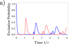
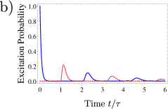
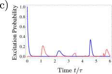
Figure 2: Atomic excitation probabilities for $\Gamma\tau=16$ and $\epsilon=1/10,\;\lambda_{eg}\ll d,f$ (a) and $\epsilon=1/2,\;\lambda_{eg}\ll d,f$ (b), $d/\lambda_{eg}=20,\;f/\lambda_{eg}=10$ (c). The excitation probability of atom 1 (2) is represented by the blue (red) curve.

In these cases the excitation probabilities of the atoms are sharply peaked in time. After the decay of the first atom the second atom is excited after time $\tau$, which is the typical time the photon needs to travel from the first atom to the second one as expected from geometrical optics. The remaining peaks in Fig. 2 a and Fig. 2 b can be understood in terms of descriptive photon paths as discussed in Sec. 4. By comparing the dynamics illustrated in Fig. 2 a with the dynamics illustrated in Fig. 2 b we can study the influence of the geometry of the cavity as already discussed in Subsec. 4.3. The situation in Fig. 2 a with ${f}/{d}={9}/{2}\Leftrightarrow\epsilon={1}/{10}$ corresponds to an almost spherical cavity. Therefore, the coupling between both atoms is relatively large. The situation in Fig. 2 b with${f}/{d}={1}/{2}\Leftrightarrow\epsilon={1}/{2}$ corresponds to a highly non spherical cavity. Thus, in accordance with the results obtained in Subsec. 4.3, the coupling between the atoms is reduced.

The semiclassical expressions obtained by the separation ansatz in Sec. 3 can also be used to study diffraction effects in cases of relatively long wavelengths ($\lambda_{eg}$ of similar order of magnitude as $d$ or $f$). Such a situation is illustrated in Fig. 2 c. The influence of diffraction effects can be illustrated by comparing Fig. 2 c and Fig. 2 b because both figures correspond to a cavity with eccentricity $\epsilon=1/2$. Due to these diffraction effects, the dynamics of the system in the regime $\lambda_{eg}\approx f,g$ is much more complicated than in the regime $\lambda_{eg}\ll f,g$. In the photon path representation those diffraction effects are connected with the appearance of additional photon paths which are not connected to geometrical optics.

Our former treatment of the extreme multimode scenario also enables us to study the transition from the extreme multimode scenario which corresponds to $\tau\Gamma\gg 1$ to the single mode regime with $\tau\Gamma\ll 1$. To keep the discussion as simple as possible, we consider the scenario of very small wavelengths and an almost spherical cavity $\lambda_{eg}\ll d\ll f$ . If we take the limit $\tau\Gamma\rightarrow 0$ with $\Gamma=\tau\Omega_{0}^{2}/2$ and $e^{\mathrm{i}2\tau\omega_{eg}}=1$, we obtain exactly the results of a single mode coupling on resonance to the two two level atoms and $\Omega_{0}$ being the vacuum Rabi frequency of a single atom coupling to this mode. In Fig. 3 we compare the single mode scenario for $\tau\rightarrow 0$ with the results for finite $\tau$ which are more complicated due to the presence of additional modes.

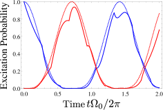
Figure 3: Comparison of atomic excitation probabilities for finite $\tau$ with ideal single mode scenario $\tau\rightarrow 0$: The dashed lines correspond to $\tau\rightarrow 0$ and the solid lines to the results for finite $\tau$. The excitation probability of atom 1 (2) is represented by the blue (red) curves. The parameters for the solid lines are $\tau=4\pi/15\Omega_{0}$.

6 Conclusion

We have investigated the dynamics of spontaneous photon emission and absorption processes of two two-level atoms trapped close to the focal points of a prolate-ellipsoidal cavity. Our theoretical approach is based on a full multimode treatment of the electromagnetic radiation field and incorporates the dipole approximation and the RWA. In order to deal with the electromagnetic radiation field in the multimode scenario, we have applied semiclassical methods by exploiting the separability of the relevant electromagnetic mode functions. With the help of the expressions obtained by our semiclassical treatment, we have developed a semiclassical photon path representation of the relevant probability amplitudes. This photon path representation enables us to discuss the dynamics inside the cavity by means of descriptive photon paths. This way, we have studied the interplay between both atoms mediated by the radiation field and have addressed intermediate instances between well-known quantum-optical scenarios. These well-known scenarios include Rabi oscillations which emerge for $\Gamma\tau\ll 1$ or an almost Markovian dynamics of the atoms dominated by spontaneous decay processes which emerge as $\Gamma\tau\gg 1$ and as the eccentricity $\epsilon$ approaches unity. We have also investigated diffraction effects and their suppression in the limit of extremely small wavelengths. This work is supported by CASED III, the BMBF Project Q.com, and by the DFG as part of the CRC 1119 CROSSING.

References

References

• [1] Berman P (ed) 1994 Cavity Quantum Electrodynamics (San Diego: Academic Press)
• [2] Walther H H et al. 2006 Prog. Phys. 69 1325
• [3] Haroche S et al. 2006 Exploring the Quantum: Atoms, Cavities and Photons (Oxford: Oxford University Press)
• [4] Goy P et al. 1983 Phys. Rev. Lett. 50 1903–1906
• [5] Meschede D et al. 1985 Phys. Rev. Lett. 54 551
• [6] McKeever J et al. 2003 Nature 425 268–271
• [7] Schleich W 2001 Quantum Optics in Phase Space (Berlin: Wiley-VCH)
• [8] Jaynes E T and Cummings F W 1963 Proceedings of the IEEE 51 89–109
• [9] Moehring D L, Maunz P, Olmschenk S, Younge K C, Matsukevich D N, Duan L M and Monroe C 2007 Nature 449 68
• [10] Olmschenk S, Matsukevich D N, Maunz P, Hayes D, Duan L M and Monroe C 2009 Science 323 486
• [11] Aljunid S, Maslennikov G, Wang Y, Dao H, Scarani V and Kurtsiefer C 2013 Phys. Rev. Lett. 111(10) 103001
• [12] Maiwald R et al. 2009 Nat. Phys. 5 551 – 554
• [13] Maiwald R et al. 2012 Phys. Rev. A 86 043431
• [14] Hétet G, Slodička L, Hennrich M and Blatt R 2011 Physical review letters 107 133002
• [15] Alber G et al. 2013 Phy. Rev. A 88 023825
• [16] Flammer C 1957 Spheroidal Wave Functions (stanford university press)
• [17] Berry M and Mount K 1972 Rep. Prog. Phys. 35 315
• [18] Abramowitz M and Stegun I 1984 Pocketbook of Mathematical Functions (Harri Deutsch)
• [19] Milonni P W and Knight P L 1974 Phy. Rev. A 10 1096–1108
• [20] Maslov V P and Fedoriuk M V 1981 Semi-Classical Approximation in Quantum Mechanics (Dordrecht: D. Reidel)