The gas distribution in the high-redshift cluster MS 1054-0321

Abstract

We investigate the gas mass distribution in the high redshift cluster MS 1054-0321 using Chandra X-ray and OCRA SZ effect data. We use a superposition of offset $\beta$-type models to describe the composite structure of MS 1054-0321. We find gas mass fractions $f_{gas}^{\mathrm{X\mbox{-}ray}}=0.087_{-0.001}^{+0.005}$ and $f_{gas}^{\mathrm{SZ}}=0.094_{-0.001}^{+0.003}$ for the (main) eastern component of MS 1054-0321 using X-ray or SZ data, but $f_{gas}^{\mathrm{X\mbox{-}ray}}=0.030_{-0.014}^{+0.010}$ for the western component. The gas mass fraction for the eastern component is in agreement with some results reported in the literature, but inconsistent with the cosmic baryon fraction. The low gas mass fraction for the western component is likely to be a consequence of gas stripping during the ongoing merger. The gas mass fraction of the integrated system is $0.060_{-0.009}^{+0.004}$: we suggest that the missing baryons from the western component are present as hot diffuse gas which is poorly represented in existing X-ray images. The missing gas could appear in sensitive SZ maps.

1 Introduction

The properties of massive high redshift clusters could place powerful constraints on the cosmological parameters that govern the physics of the early Universe (Joy et al., 2001; Brodwin et al., 2012). Several studies have used clusters at high redshift to provide valuable information on galaxy formation and evolution in the richest environments and to probe Gaussianity in the density field that seeded structure formation (Foley et al., 2011; Wen & Han, 2011; Brodwin et al., 2012). Massive clusters, with $M_{tot}\sim 10^{15}\,\mathrm{M_{\odot}}$, are identified by their gravitational lensing of background galaxies (Zaritsky & Gonzalez, 2003; Medezinski et al., 2011), and by the X-ray emission or Sunyaev-Zel’dovich effect (SZ) from their hot intracluster medium (ICM) (Morandi, Ettori & Moscardini, 2007; Battaglia et al., 2012).

The X-ray emission from diffuse hot plasma at $T>5\,\mathrm{keV}$ is primarily bremsstrahlung from the gas within the potential well of the cluster’s dark matter halo. The X-ray luminosity is proportional to the square of the electron density, hence is sensitive to the denser regions of the cluster. On the other hand, the thermal SZ effect, the change in the brightness of the cosmic microwave background caused by hot electrons in the ICM inverse-Compton scattering, depends on the ICM pressure (the integrated product of the electron density and temperature on the line of sight). This parameter dependence makes the SZ effect a powerful tool to probe lower-density regions of the hot gas, and thus to provide better insight into gas properties outside the cluster core or in the hottest regions. For reviews of the physics of the SZ effect see Rephaeli (1995), Birkinshaw (1999), and Carlstrom, Holder & Reese (2002). Due to the different sensitivity of the SZ effect and the X-ray emission to outer and inner regions of the cluster, these two independent probes can be used to provide a more complete picture of the ICM. By combining X-ray and SZ effect data, the distance of the cluster can be estimated and hence the Hubble constant or other cosmological parameters can be found (e.g. Birkinshaw, Hughes & Arnaud, 1991; Worrall & Birkinshaw, 2003; Bonamente et al., 2006). Alternatively, tight constraints on the gas mass fraction of the cluster can be obtained (see Grego et al., 2001; LaRoque et al., 2006; Planck Collaboration, 2013, for example).

Observations with X-ray satellites such as Chandra and XMM–Newton have provided high quality images of the X-ray emission and detailed structural properties of the ICM (e.g. Vikhlinin et al., 2006; Pratt et al., 2009). In parallel, many SZ observatories such as the South Pole Telescope (SPT, Carlstrom et al., 2011), and the One Centimeter Receiver array (OCRA, Lancaster et al., 2011) have made high signal-to-noise SZ measurements toward clusters. Generally the models used to interpret SZ effect have been rather simple.

In this paper we investigate the gas mass distribution of the high redshift cluster MS 1054-0321, taking advantage of a long Chandra observation of MS 1054-0321 and high signal/noise SZ effect data from OCRA, to develop a three-dimensional gas density profile of the $\beta$-model type. We use this to improve the measurement of the gas mass of MS 1054-0321. The physical properties of the gas of MS 1054-0321 were analysed in previous studies. However in most of these studies, standard isothermal $\beta$-models were used for the cluster plasma distribution although the structure of the cluster is clearly more complicated. Since the ICM mass and the total mass of cluster are functions of temperature, we also re-analyse the X-ray temperature structure of MS 1054-0321. We use our results to estimate the gas and total masses of the cluster.

In the next Section we review MS 1054-0321. In Section 3 we describe the X-ray and radio observations of MS 1054-0321. The analysis method for 3D single-$\beta$ and double-$\beta$ models used to describe the plasma distribution is presented in Section 4. The gas mass content of MS 1054-0321 is discussed in Section 5. Finally, in Section 6 we summarise our results. Throughout this paper, we use a $\Lambda$CDM cosmology with $\Omega_{\mathrm{m}}=0.3$, $\Omega_{\Lambda}=0.7$, and $H_{0}=100\,h_{100}\,\mathrm{km\,sec^{-1}\,Mpc^{-1}}$ with $h_{100}=0.7$. Uncertainties are at the 68% confidence level, unless otherwise stated.

2 CLUSTER MS 1054-0321

The rich cluster MS 1054-0321 is the most distant and luminous cluster in the Einstein Extended Medium Sensitivity Survey (EMSS, Gioia et al., 1990). Due to its high redshift ($z$ = 0.83 corresponding to angular diameter distance $D_{A}=1.57\,\mathrm{Gpc}$) and complicated morphology, the ICM plasma of MS 1054-0321 has been subjected to many studies. X-ray observations of MS 1054-0321 with the ASCA and ROSAT satellites were analysed by Donahue et al. (1998). The ASCA spectrum showed a high X-ray temperature of $12.3^{+3.1}_{-2.2}\,\mathrm{keV}$ ($90\%$ confidence interval), which should indicate that MS 1054-0321 is a massive cluster. The X-ray image from the ROSAT HRI identified two or three components in addition to an extended component, suggesting that MS 1054-0321 is not in a relaxed state. Based on this X-ray temperature and using the mass-temperature relation adopted from the simulations of Evrard, Metzler & Navarro (1996), the virial mass of MS 1054-0321 estimated by Donahue et al. (1998) was $\sim 7.4\times 10^{14}\,h_{100}^{-1}\,\mathrm{M_{\odot}}$ within a region of a radius $r_{200}=1.5\,h_{100}^{-1}\,\mathrm{Mpc}$.

The ROSAT HRI observation of MS 1054-0321 was re-analysed by Neumann & Arnaud (2000) and new HRI data were included in order to gain better insight into the main components of MS 1054-0321. These authors found evidence for a significant clump to the west of the main component of the cluster. The HRI image was fitted to 1D spherical and 2D elliptical $\beta$-models. Excluding the western component, Neumann & Arnaud found the best fit to the 1D spherical model to have $\beta=0.96_{-0.22}^{+0.48}$ and $r_{c}=442_{-104}^{+184}\,h_{50}^{-1}\,\mathrm{kpc}$. However, if the western substructure is included, the best spherical model fit gives $\beta=2$ and $r_{c}=840\,h_{50}^{-1}\,\mathrm{kpc}$ with large errors. On the other hand, an elliptical $\beta$-model fits the main cluster component with $\beta=0.73\pm 0.18$, $r_{c1}=(422\pm 109)\,h_{50}^{-1}\,\mathrm{kpc}$ and $r_{c2}=(298\pm 65)\,h_{50}^{-1}\,\mathrm{kpc}$. Considering only the main component of MS 1054-0321 and using the best fit temperature from the ASCA spectrum, Neumann & Arnaud (2000) derived gas masses inside $1.65\,h_{50}^{-1}\,\mathrm{Mpc}$ of $(1.9\pm 0.3)\times 10^{14}\,h_{50}^{-5/2}\,\mathrm{M_{\odot}}$ and $2.5\times 10^{14}\,h_{50}^{-5/2}\,\mathrm{M_{\odot}}$ from the best fit parameters of the 1D and 2D beta models, respectively. They estimated total masses of MS 1054-0321 at $1.65\,h_{50}^{-1}\,\mathrm{Mpc}$ of $2.0_{-0.4}^{+0.8}\times 10^{15}\,h_{50}^{-5/2}\,\mathrm{M_{\odot}}$ and $1.6\times 10^{15}\,h_{50}^{-5/2}\,\mathrm{M_{\odot}}$ from the 1D and 2D $\beta$-models, respectively. The gas mass fraction is then about $0.10\,h_{50}^{-3/2}$ or $0.16\,h_{50}^{-3/2}$, depending on the choice of model.

Jeltema et al. (2001) analysed a Chandra ACIS-S observation of MS 1054-0321. They estimated the X-ray temperature for the entire cluster to be $10.4_{-1.5}^{+1.7}\,\mathrm{keV}$, and confirmed the substructure in the ROSAT HRI data. The eastern clump is almost coincident with the main component of the cluster, and has an X-ray temperature of $10.5_{-2.1}^{+3.4}\,\mathrm{keV}$. The western clump is more compact and denser than the eastern clump, with a temperature of $6.7_{-1.2}^{+1.7}\,\mathrm{keV}$. The quoted errors are at $90\%$ confidence ranges for the two-parameter fit. Using the temperature of the whole cluster,  Jeltema et al. estimated a virial mass of $\sim 6.2_{-1.3}^{+1.6}\times 10^{14}\,h_{100}^{-1}\,\mathrm{M_{\odot}}$ within $r_{200}=0.76\,h_{100}^{-1}\,\mathrm{Mpc}$. The authors also estimated the total mass using a $\beta$-model (setting $\beta=1$ and fitting for the cluster core radius), and obtained a mass of $7.4\times 10^{14}\,h_{100}^{-1}\,\mathrm{M_{\odot}}$ within $r_{200}$.

An investigation of the temperature structure of MS 1054-0321 using XMM–Newton (Gioia et al., 2004) indicated a temperature for the whole cluster of $7.2_{-0.6}^{+0.7}\,\mathrm{keV}$, lower than any of the temperatures reported previously. The two significant clumps already seen by the ROSAT and the Chandra satellites were also seen in the XMM–Newton data. As in the result reported by Jeltema et al. (2001), the eastern clump has the higher temperature, $8.1_{-1.2}^{+1.3}\,\mathrm{keV}$, consistent with the integrated cluster temperature, and the western clump, at $5.6_{-0.6}^{+0.8}\,\mathrm{keV}$, is 30$\%$ cooler than the eastern clump. Quoted confidence limits are $90\%$ for one interesting parameter.

Jee et al. (2005) analysed HST ACS weak-lensing and Chandra X-ray data of MS 1054-0321. The dark matter structure mainly consists of three dominant clumps with a few minor satellite groups. The eastern weak-lensing clump from the mass map is not detected in the X-ray data, and the two X-ray clumps are displaced on the apparent merger axis relative to the central and western weak-lensing substructures, probably due to ram pressure.  Jee et al. estimated the projected mass to be $(7.14\pm 0.11)\times 10^{14}\,h_{100}^{-1}\,\mathrm{M_{\odot}}$ at $r=1\,\mathrm{Mpc}$, consistent with previous lensing work (Luppino & Kaiser, 1997; Hoekstra, Franx & Kuijken, 2000). They also fitted the X-ray surface brightness of MS 1054-0321 to an isothermal 1D $\beta$-model, excluding the core region ($r<45\arcsec$) from the fit, to find $\beta=0.78\pm 0.08$ and $r_{c}=(16\pm 15)\arcsec$, corresponding to $(85\pm 80)\,h_{100}^{-1}\,\mathrm{kpc}$ in our adopted cosmology. Using an X-ray temperature of $8.9_{-0.8}^{+1.0}\,\mathrm{keV}$,  Jee et al. found the mass within radius 1 Mpc is $(8.4\pm 0.14)\times 10^{14}\,h_{100}^{-1}\,\mathrm{M_{\odot}}$, agreeing with their weak-lensing result.

Using OVRO/BIMA interferometric SZ effect data, Joy et al. (2001) estimated the gas mass of MS 1054-0321 within a radius of $94\arcsec$ ($501\,h_{100}^{-1}\,\mathrm{kpc}$ in our adopted cosmology) to be $(3.7\pm 0.6)\times 10^{13}\,h_{100}^{-2}\,\mathrm{M_{\odot}}$ for a temperature of $10.4_{-2.0}^{+5.0}\,\mathrm{keV}$. Using the mean gas mass fraction of a sample of galaxy clusters reported by Grego et al. (2001), the derived total mass was $(4.6\pm 0.8)\times 10^{14}\,h_{100}^{-1}\,\mathrm{M_{\odot}}$ within the same radius. LaRoque et al. (2006) derived the gas mass fraction within $r_{2500}$ for a sample of massive clusters including MS 1054-0321 from Chandra together with OVRA/BIMA data using three different models for the plasma distribution. The first model, the isothermal $\beta$-model fit to the X-ray data at radius beyond 100 kpc and to all of the SZ effect data, yielded $f_{\mathrm{gas}}^{\mathrm{X\mbox{-}ray}}=0.144_{-0.013}^{+0.014}$ and $f_{\mathrm{gas}}^{\mathrm{SZ}}=0.153_{-0.029}^{+0.034}$. The second model, the nonisothermal double $\beta$-model fit to all of the X-ray and SZ effect data, gave $f_{\mathrm{gas}}^{\mathrm{X\mbox{-}ray}}=0.106_{-0.010}^{+0.009}$ and $f_{\mathrm{gas}}^{\mathrm{SZ}}=0.102_{-0.018}^{+0.020}$. The third, the isothermal $\beta$-model fit to the SZ data with $\beta$ fixed at 0.7, yielded $f_{\mathrm{gas}}^{\mathrm{SZ}}=0.187_{-0.054}^{+0.081}$. Performing a joint fit analysis of the same X-ray and SZ effect data, Bonamente et al. (2008) determined the gas mass fraction of MS 1054-0321 using an isothermal $\beta$-model excluding the central region (100 kpc) from the X-ray data. They found the gas mass fraction within $89\arcsec$ ($475\,h_{100}^{-1}\,\mathrm{kpc}$ in our adopted cosmology) to be $0.164\pm 0.019$.

In Table 1 we summarize the reported measurements of the physical properties of MS 1054-0321. The numerical values of these measurements are converted to the cosmology adopted by this work. As can be seen, the results are not entirely consistent.

Table 1: The physical properties of MS 1054-0321 reported in the literature.

Study	Method	Radius	$M_{gas}$	$M_{tot}$	$f_{gas}$
		$(h_{100}^{-1}\,\mathrm{Mpc})$	$(10^{13}\,h_{100}^{-1}\,\mathrm{M_{\odot}})$	$(10^{14}\,h_{100}^{-1}\,\mathrm{M_{\odot}})$
Donahue et al. (1998)	$M$-$T$ relation	$r_{200}=1.50$	—	7.4	—
Neumann & Arnaud (2000)	$\beta$-model	1.16	$13.30\pm 2.10$	$14.00_{-2.80}^{+5.60}$	0.095
	Elliptical $\beta$-model2nd_fnt	1.16	17.50	11.20	0.156
Grego et al. (2001)	$\beta$-model	$r_{500}=0.86$	—	—	$0.053\pm 0.028$
Joy et al. (2001)	$\beta$-model3rd_fnt	0.50	$5.29\pm 0.86$	$4.60\pm 0.80$	$0.115_{-0.016}^{+0.013}$
Jeltema et al. (2001)	$M$-$T$ relation	$r_{200}=0.76$	—	6.21st_fnt	—
	$\beta$-model	$r_{200}=0.76$	—	7.4	—
Jee et al. (2005)	Weak-lensing	0.7	—	$7.14\pm 0.11$	—
	$\beta$-model	0.7	—	$8.40\pm 0.14$	—
LaRoque et al. (2006)	$\beta$-model	$r_{2500}\approx 0.18$	$0.74_{-0.34}^{+0.35}$	$0.52_{-0.27}^{+0.32}$	$0.144_{-0.013}^{+0.014}$
			$0.78_{-0.33}^{+0.29}$	$0.52_{-0.27}^{+0.32}$	$0.153_{-0.029}^{+0.034}$
	Double $\beta$-model	$r_{2500}\approx 0.18$7th_fnt	$0.74\pm 0.18$	$0.70_{-0.20}^{+0.24}$	$0.106_{-0.010}^{+0.009}$
			$0.72\pm 0.11$	$0.70_{-0.20}^{+0.24}$	$0.102_{-0.018}^{+0.020}$
	$\beta$-model	$r_{2500}\approx 0.18$7th_fnt	$0.82\pm 0.11$	$0.43_{-0.11}^{+0.15}$	$0.187_{-0.054}^{+0.081}$
Bonamente et al. (2008)	$\beta$-model6th_fnt	$r_{2500}=0.48$	$5.18_{-0.70}^{+0.84}$	$3.15_{-0.70}^{+0.98}$	$0.164\pm 0.019$

3 DATA

3.1 The X-ray image

We used archival data for MS 1054-0321 from the same Chandra ACIS-S observation in April 2000 used by Jeltema et al. (2001) and Jee et al. (2005). The total observation duration was 90 ks. Chandra Interactive Analysis of Observations (CIAO) version 4.5, with calibration database (CALDB) version 4.5.9, was used to reduce the X-ray data. The data were reprocessed by running the chandra_repro script to create a new level = 2 event file, and a new bad pixel file. To minimize the high energy particle background, counts were considered only in the energy range 0.5-7.0 keV. X-ray background counts were obtained from the local background on the Chandra ACIS-S3 chip. Point sources on this chip were detected, removed, and replaced by a local estimate of the background emission. Our image of the X-ray surface brightness of MS 1054-0321 is shown in Fig. 1. This image is smoothed by a two-dimensional Gaussian kernel with $\sigma=3.44\arcsec$.

The X-ray structure of the cluster shows an elliptical shape elongated in the east-west direction with two main components, indicated by two green boxes labelled E and W. The eastern component is relatively diffuse and less bright at its centre, which lies around $5\arcsec$ (40 kpc) from the position of the cluster brightest optical galaxy (Best et al., 2002). The western component is more compact, has a higher X-ray surface brightness, and its peak is separated from the peak of the eastern component by $\sim 55\arcsec$ (420 kpc).

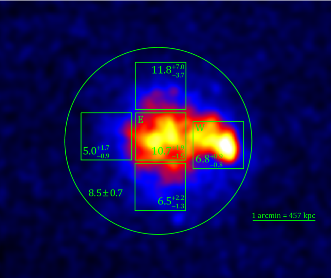
Figure 1: Chandra X-ray image of the cluster MS 1054-0321 in the 0.5-7.0 keV energy band smoothed by a Gaussian of $\sigma=3.44\arcsec$ (26 kpc). The green circle and boxes show the regions in which the X-ray temperatures were extracted. Numerical values are the best-fit temperatures in units of keV for given regions. The E and W letters denote the eastern and western components of the cluster discussed in the main text.

3.2 The X-ray spectra

The emission weighted temperature of the whole cluster was obtained by using counts ($\sim$ 14120 counts between 0.5 and 7.0 keV) from a circular region of radius $90\arcsec$ centred at (RA, Dec) = ($10^{\mathrm{h}}57^{\mathrm{m}}00\aas@@fstack{s}02$, $-03\degr 37\arcmin 36\aas@@fstack{\prime\prime}00$). This corresponds to the position of the optically brightest galaxy in the cluster (Best et al., 2002). We fitted the X-ray spectrum with a MEKAL model (Mewe, Gronenschild & van den Oord, 1985) modified by local Galactic absorption after binning the counts to at least 30 per energy bin. The iron abundance and the temperature were left free to vary, whereas the Galactic absorption and the cluster redshift were constrained at $3.67\times 10^{20}\,\mathrm{atoms\,cm^{-2}}$ (Dickey & Lockman, 1990) and 0.83 (van Dokkum et al., 2000), respectively. The best fit yields a temperature $T=8.5\pm 0.7\,\mathrm{keV}$ and a metal abundance $Z=0.33\pm 0.11\,Z_{\odot}$ at 68% confidence level, with a reduced $\chi^{2}=0.74$ for 215 degrees of freedom. Our temperature estimate is in good agreement with the Chandra temperature reported by Jee et al. (2005) ($T=8.9_{-0.8}^{+1.0}\,\mathrm{keV}$) and by Tozzi et al. (2003) ($T=8.0\pm 0.5\,\mathrm{keV}$), and also with the XMM–Newton temperature, $T=7.2_{-0.6}^{+0.7}\,\mathrm{keV}$ ($90\%$ confidence limits), presented by Gioia et al. (2004). However, it is slightly lower than the Jeltema et al. (2001) value, based on the same Chandra data $(T=10.4_{-1.5}^{+1.7}\,\mathrm{keV}$ at $90\%$ confidence limits), and much lower than the ASCA temperature, $T=12.3_{-2.2}^{+3.1}\,\mathrm{keV}$ ($90\%$ confidence limits), determined by Donahue et al. (1998). The metal abundance obtained from our fitting of the X-ray spectrum agrees with previous results reported by Gioia et al. (2004) ($Z=0.33_{-0.18}^{+0.19}\,Z_{\odot}$ at $90\%$ confidence limits) and by Jee et al. (2005) ($Z=0.30\pm 0.12\,Z_{\odot}$).

We also investigated the temperatures of the densest parts of the eastern and western components by extracting counts from the regions with size of $48.71\arcsec\times 45.46\arcsec$, centred at RA = $10^{\mathrm{h}}56^{\mathrm{m}}59\aas@@fstack{s}87$, Dec = $-03\degr 37\arcmin 31\aas@@fstack{\prime\prime}68$, and RA = $10^{\mathrm{h}}56^{\mathrm{m}}56\aas@@fstack{s}16$, Dec = $-03\degr 37\arcmin 39\aas@@fstack{\prime\prime}95$ (Fig. 1). There are around 3090 and 2725 counts in the energy range of 0.5-7.0 keV in the eastern and western components, respectively. The X-ray data again were fitted with a MEKAL model, with Galactic absorption frozen at $3.67\times 10^{20}\,\mathrm{atoms\,cm^{-2}}$ and the cluster redshift frozen at 0.83. The temperature and the metal abundance were left free to vary. The best fit for the eastern component gives a temperature $T=10.7_{-1.5}^{+1.9}\,\mathrm{keV}$ and an abundance $Z=0.11_{-0.11}^{+0.22}\,Z_{\odot}$ with a reduced $\chi^{2}=0.71$ for 72 degrees of freedom. For the western component, the best fit gives a temperature $T=6.8_{-0.8}^{+0.9}\,\mathrm{keV}$ and an abundance $Z=0.34_{-0.19}^{+0.20}\,Z_{\odot}$ with a reduced $\chi^{2}=0.66$ for 67 degrees of freedom. The X-ray spectra with the best fit models of the full cluster, the eastern and western components are shown in Fig. 2. All the spectra were binned to 30 or more counts per energy bin.

Our temperature measurements clearly show that the eastern component is hotter than the western component. Such results are fully consistent with the temperatures of the eastern and western components reported by Jee et al. (2005) ($T=10.7_{-1.7}^{+2.1}\,\mathrm{and}\,7.5_{-1.2}^{+1.4}\,\mathrm{keV}$), and by Jeltema et al. (2001) ($T=10.5_{-2.1}^{+3.4}\,\mathrm{and}\,6.7_{-1.2}^{+1.7}\,\mathrm{keV}$ at $90\%$ confidence limits). Gioia et al. (2004) also noticed the significant difference of temperature between the eastern and western components ($T=8.1_{-1.2}^{+1.3}\,\mathrm{and}\,5.6_{-0.6}^{+0.8}\,\mathrm{keV}$ at $90\%$ confidence limits), but their temperatures are systematically lower than our values. Our results for the abundance agree with eastern and western component values obtained by Jee et al. (2005) ($Z=0.16_{-0.16}^{+0.19}$ and $0.47_{-0.23}^{+0.24}\,Z_{\odot}$), and by Gioia et al. (2004) ($Z=0.12_{-0.12}^{+0.35}$ and $0.51_{-0.32}^{+0.36}\,Z_{\odot}$ at $90\%$ confidence limits). Jeltema et al. (2001) reported similar results, ($Z=0.08_{-0.08}^{+0.23}$ and $0.46_{-0.26}^{+0.27}\,Z_{\odot}$ at $90\%$ confidence limits), relative to the slightly different solar iron abundance of Anders & Grevesse (1989).

The significant variation in temperature between these two components led us to investigate the temperature structure for other regions within the cluster atmosphere. Thus, we extracted counts from three regions to the north, south, and east of the eastern component (see Fig. 1). The size of each region was chosen to be equivalent to that of the eastern (or western) component, and their centres are about $50\arcsec$ (380 kpc) away from the centre of the eastern component. There are around 1040, 1430, and 890 counts in the energy range 0.5-7.0 keV in the north, south, and east regions, respectively. The X-ray spectrum in each region was binned to include at least 50 counts per bin. The X-ray data were then fitted to a MEKAL model modified by a local Galactic absorption. Galactic absorption and the cluster redshift were fixed as before, whereas the temperature and the metal abundance were left free to vary. The best fit for the region north of the eastern component gives a temperature $T=11.8_{-3.7}^{+7.0}\,\mathrm{keV}$ and an abundance $Z=0.76_{-0.76}^{+1.33}\,Z_{\odot}$ with a reduced $\chi^{2}=1.39$ for 15 degrees of freedom. For the region to the south, the best fit yields a temperature $T=6.5_{-1.3}^{+2.2}\,\mathrm{keV}$ and an abundance $Z=0.38_{-0.38}^{+0.46}\,Z_{\odot}$ with a reduced $\chi^{2}=0.91$ for 22 degrees of freedom. The best fit temperature and abundance for the region to the east are $T=5.0_{-0.9}^{+1.7}\,\mathrm{keV}$ and $Z=2.20_{-1.21}^{+2.19}\,Z_{\odot}$ with a reduced $\chi^{2}=1.08$ for 13 degrees of freedom.

These results indicate that the temperature of the eastern component decreases by a factor $\sim 2$ over scale $\sim 50\arcsec$ (380 kpc), except to the north, where a lesser, or no, temperature change is found. Fixing the metallicity at the cluster central value leads to higher outer temperatures in the east and south, and lower temperature gradients. If the Galactic hydrogen column is allowed to be free, then we obtain fits of equivalent quality to these found with fixed $N_{H}$, but with best-fit temperatures $\sim 1\,\mathrm{keV}$ higher in all cases. However, the fitted values of $N_{H}$ are below the known Galactic column, and so we don’t consider these results further.

3.3 The Sunyaev-Zel’dovich effect data

MS 1054-0321 was observed at 30 GHz over the period 28 February 2006 to 2 June 2006 using the Toruń 32 m telescope equipped with the prototype One Centimetre Receiver Array (OCRA-p) (Lancaster et al., 2007). OCRA-p consists of two 1.2 arcmin FWHM beams separated by 3.1 arcmin, and can achieve 5 mJy sensitivity in 300 seconds. OCRA-p observed MS 1054-0321 for $\sim 11$ hours using a combination of beam-switching and position-switching. Such a technique is efficient at subtracting atmospheric and ground signals, and removes such contaminating signals better than position-switching or beam-switching alone (Birkinshaw & Lancaster, 2008). The principles of the beam- and position-switching technique and the data reduction process are described in detail in Lancaster et al. (2007).

The OCRA data were calibrated by reference to two bright radio sources NGC7027 and 3C286, with flux densities of 5.64 and 2.51 Jy. By reprocessing the OCRA data for the MS 1054-0321 cluster, we estimated the SZ effect toward the cluster centre to be $-2.18\pm 0.33\,\mathrm{mJy}$ with standard deviation of individual 1-minute records $\sigma=5.16\,\mathrm{mJy}$. This central measured SZ flux density could be increased or decreased by the emission of radio sources. An investigation of radio point sources in the MS 1054-0321 field and their impact on the SZ effect measurement is presented below.

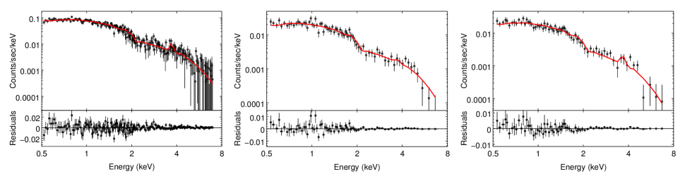
Figure 2: Binned X-ray spectra for MS 1054-0321. Left: The full cluster. Centre: the eastern component. Right: the western component. The solid line is the best fit thermal plasma model. It is clear that the emission line of iron is more evident in the wastern component than the eastern component. Lower panels: the residuals from the best fit model.

3.4 The radio environment

Point source contamination is a major problem in low-resolution observations of the SZ effect. For the two-beam receiver, OCRA-p, radio sources could lead to an overestimate of the SZ effect if they are located in the reference background regions of the observation. Radio sources lead to an underestimate of the SZ signal when they lie along the line of the sight to the cluster. By knowing the flux densities and locations of radio point sources near our pointing centre at our observing frequency, we can correct for them and improve our estimate of the SZ effect of the cluster. Currently, a sensitive survey of the radio sky at 30 GHz does not exist, but the radio field of the cluster MS 1054-0321 has been observed at multiple bands. Hence we estimate the flux densities at 30 GHz of the radio sources in the field of MS 1054-0321 by extrapolating from lower frequency measurements. We use flux densities from the NRAO VLA Sky Survey (NVSS) (1.4 GHz, Condon et al., 1998), and the 28.5 GHz flux densities for sources near the cluster centre reported in Coble et al. (2007). We also use flux density measurements at 4.85 GHz by reprocessing archival VLA data. In all fields, only the radio sources within a radius of 4.5 arcmin from the centre of the cluster are considered, and we neglect possible radio source variability.

We find four significant radio point sources in the field of the MS 1054-0321 cluster. One is located close to the cluster centre, and another is found outside the reference arc of the beam-switched observation. The two remaining sources are found in the reference arc, and they could produce a negative signal that boosts the apparent SZ effect. All four point sources have 1.4 GHz flux density measurements. Measurements at 28.5 GHz are available only for the inner three sources.

The archival VLA data were taken at 4835 and 4885 MHz with 50 MHz bandwidth. We reduced the data using the Astronomical Image Processing System (AIPS). The source 3C286 = 1331+305 was used as the primary calibrator to calibrate the flux density, with flux densities of 7.51 and 7.46 Jy. Source 1058+015 was the phase calibrator, and was observed at around 30 minute intervals throughout the observation. After the normal calibration and imaging steps, the position, peak intensity, and total flux density of the detected radio sources were estimated using the IMFIT task, after correction for the VLA primary beam.

We estimated the flux densities of the radio sources at 30 GHz by fitting a power law to the measurements and extrapolating to 30 GHz. The flux densities and positions of the four radio sources within 4.5 arcmin of the pointing centre of the MS 1054-0321 cluster are given in Table 2. These values are essentially the same as those given by Coble et al. (2007) at 28.5 GHz, except for source 4 which is not in their list.

Table 2: The radio source fluxes within 4.5 arcmin from the pointing centre of the cluster MS 1054-0321. From left to right the columns give the source identification number, the right ascension and declination of the radio source, the flux density at 1.4 GHz (from Condon et al. 1998), the flux density at 4.8 GHz after primary beam correction, the flux density at 28.5 GHz (from Coble et al. 2007), the expected flux density at 30 GHz.

Source ID	RA	Dec	$S_{1.4}$	$S_{4.85}$	$S_{28.5}$	$S_{30}$
	(J2000)	(J2000)	(mJy)	(mJy)	(mJy)	(mJy)
1	10 56 59.59	-03 37 27.7	$14.10\pm 0.90$	$7.28\pm 0.10$	$0.94\pm 0.06$	$0.87\pm 0.06$
2	10 56 57.94	-03 38 58.3	$3.10\pm 0.40$	$1.29\pm 0.12$	$0.54\pm 0.08$	$0.48\pm 0.07$
3	10 56 48.85	-03 37 28.8	$18.20\pm 1.00$	$4.41\pm 0.20$	$1.79\pm 0.19$	$1.75\pm 0.19$
4	10 56 48.59	-03 40 07.1	$4.64\pm 0.40$	$2.79\pm 0.22$	—	$1.36\pm 0.31$

3.5 Radio source corrections

We correct our central SZ effect measurement using the flux densities and positions of the point sources. The greatest contamination comes from source 3, which is observed in the reference arc at parallactic angle $\sim 5\degr$. Source 1 is un-modulated by the changing parallactic angle during beam-switching, while source 4 has little effect since it lies far from the sampled reference arc. The corrected value of the central SZ effect flux density of MS 1054-0321 is $-2.55\pm 0.33\,\mathrm{mJy}$, indicating an effect about $1\sigma$ greater than our uncorrected value, and consistent with a massive hot atmosphere.

4 MODELING

4.1 Cluster atmosphere

The X-ray surface brightness, $S_{X}$, and the Sunyaev-Zel’dovich effect, $\Delta T$, of a cluster can be expressed as functions of the electron density, $n_{e}$, and electron temperature, $T_{e}$, of the intracluster plasma integrated along the line of sight

$$S_{X}={{1}\over{4\pi(1+z)^{4}}}D_{A}\int n_{e}^{2}\Lambda_{ee}d\theta_{z},$$ (1)

and

$$\Delta T=f(x)T_{r}{{k_{B}\sigma_{T}}\over{m_{e}c^{2}}}D_{A}\int n_{e}T_{e}d\theta_{z}.$$ (2)

$D_{A}$ is the angular diameter distance, $z$ (=0.83) is the cluster redshift, $\Lambda_{ee}$ is the X-ray spectral emissivity of the cluster plasma, $f(x)$ describes the frequency dependence of the SZ effect and has value $-1.91$ at our observing frequency. $T_{r}$ (= 2.725 K, Fixsen, 2009) is the temperature of the cosmic microwave background radiation, $k_{B}$ is the Boltzmann constant, $\sigma_{T}$ is the Thomson scattering cross section, $m_{e}$ is the electron mass, $c$ is the speed of light, and the integration is taken over the line of sight expressed in angular terms, $d\theta_{z}$. In order to take into account the cluster plasma distribution in both components of the MS 1054-0321 cluster, we develop an offset-centred version of a three-dimensional double $\beta$-model. A centred double $\beta$-model is often used to fit the X-ray surface brightness for clusters that show centrally-enhanced density profiles. One component describes the cluster-centred density peak, while the second component is flatter and describes the outer part of the cluster. Bonamente et al. (2006) and LaRoque et al. (2006) used a spherical double $\beta$-model to describe density profiles of cool core clusters. In this work we use a double $\beta$-model to fit the eastern and western components of the MS 1054-0321 cluster which are centred at positions separated by $\sim 55\arcsec$.

Our three dimensional double $\beta$-model of the electron density is of the form

$$n_{e}=n_{e1}+n_{e2}\hskip 140.50024pt$$

$$=n_{e01}\Big{(}1+{{\theta_{x1}^{2}}\over{\theta_{cx1}^{2}}}+{{\theta_{y1}^{2}}\over{\theta_{cy1}^{2}}}+{{(\theta_{z}-\delta)^{2}}\over{\theta_{cz1}^{2}}}\Big{)}^{-3\beta_{1}/2}$$

$$+\,n_{e02}\Big{(}1+{{\theta_{x2}^{2}}\over{\theta_{cx2}^{2}}}+{{\theta_{y2}^{2}}\over{\theta_{cy2}^{2}}}+{{\theta_{z}^{2}}\over{\theta_{cz2}^{2}}}\Big{)}^{-3\beta_{2}/2},\hskip 20.00003pt$$ (3)

and

$$\left(\begin{array}[]{c}\theta_{xn}\\ \theta_{yn}\end{array}\right)=\left(\begin{array}[]{ccc}\cos\alpha_{n}&\sin\alpha_{n}\\ -\sin\alpha_{n}&\cos\alpha_{n}\end{array}\right)\left(\begin{array}[]{c}\Theta_{x}-\Theta_{x0n}\\ \Theta_{y}-\Theta_{y0n}\end{array}\right),$$ (4)

where $n$ takes values of 1 and 2, corresponding to the eastern or western component. $n_{e01}$ and $n_{e02}$ are the central electron densities of the eastern and western components, $\beta_{1}$ and $\beta_{2}$ describe the shapes of the plasma distributions of the eastern and western components, ($\theta_{cx1}$, $\theta_{cy1}$, $\theta_{cz1}$) and ($\theta_{cx2}$, $\theta_{cy2}$, $\theta_{cz2}$) are the angular core radii of the eastern and western components. $\delta$ is the offset between the two components along the line of sight, $\alpha_{n}$ describes the rotation angle of the $xy$-plane of each component relative to an observer frame, ($\Theta_{x}$, $\Theta_{y}$) are angular coordinates, and ($\Theta_{x0n}$, $\Theta_{y0n}$) are the component centre coordinates.

This is not a general triaxial $\beta$-type model, but is adequate to describe the X-ray and Sunyaev-Zel’dovich surface brightnesses of the MS 1054-0321 cluster. Under the assumption of an isothermal intracluster medium, with the electron temperature equal to the central temperature ($T_{en}=T_{e0n}$), the X-ray spectral emissivity becomes a constant over each component ($\Lambda_{ee}=\Lambda_{een}$). For non-overlapping atmospheres, the angular structures of the X-ray surface brightness and Sunyaev-Zel’dovich effect profile for each component can be expressed as

$$S_{Xn}\propto\sqrt{\pi}{{\Gamma(3\beta_{n}-{{1}\over{2}})}\over{\Gamma({3\beta_{n}})}}\theta_{czn}\hskip 100.00015pt$$

$$\times\Big{(}1+{{\theta_{xn}^{2}}\over{\theta_{cxn}^{2}}}+{{\theta_{yn}^{2}}\over{\theta_{cyn}^{2}}}\Big{)}^{(1/2)-3\beta_{n}},$$ (5)

and

$$\Delta T_{n}\propto\sqrt{\pi}{{\Gamma({{3}\over{2}}\beta_{n}-{{1}\over{2}})}\over{\Gamma({{{3}\over{2}}\beta_{n}})}}\theta_{czn}\hskip 100.00015pt$$

$$\times\Big{(}1+{{\theta_{xn}^{2}}\over{\theta_{cxn}^{2}}}+{{\theta_{yn}^{2}}\over{\theta_{cyn}^{2}}}\Big{)}^{(1/2)-(3/2)\beta_{n}},$$ (6)

respectively. Any overlap between the atmospheres of the two components will produce a further X-ray emission contribution $\propto\int n_{e1}n_{e2}d\theta_{z}$.

Accordingly, if we can approximate the structure in terms of two distinct components (i.e., if the clusters are separated significantly beyond the largest core radius), the X-ray and SZ effect central densities for each cluster component can be obtained using

$$n_{e0n}^{\mathrm{X\mbox{-}ray}}=\Big{[}{{S_{X0n}4\pi(1+z)^{4}}\over{\Lambda_{een}\sqrt{\pi}D_{A}\theta_{czn}}}{{\Gamma({3\beta_{n}})}\over{\Gamma({3\beta_{n}-{{1}\over{2}}})}}\Big{]}^{1/2},$$ (7)

and

$$n_{e0n}^{\mathrm{SZ}}={{\Delta T_{0n}m_{e}c^{2}}\over{T_{r}f(x)k_{B}T_{e0n}\sigma_{T}\sqrt{\pi}D_{A}\theta_{czn}}}{{\Gamma({{{3}\over{2}}\beta_{n}})}\over{\Gamma({{{3}\over{2}}\beta_{n}-{{1}\over{2}}})}},$$ (8)

respectively. In these equations $S_{X0n}$ and $\Delta T_{0n}$ are the central X-ray surface brightness and SZ effect signal of each cluster component.

4.2 Cluster gas and total masses

The total number of electrons in the cluster can be calculated by integrating the electron density profile over a given volume. The cluster gas mass can be obtained by multiplying the total number of electrons by the mean mass per electron, $\mu_{e}m_{p}$, so that the gas mass for each component of the cluster in some volume takes the form

$$M_{gas}(\theta_{xn},\theta_{yn},\theta_{z})=\mu_{e}m_{p}D_{A}^{3}\int\!\!\!\!\!\int\!\!\!\!\!\int n_{en}d\theta_{xn}d\theta_{yn}d\theta_{z}.$$ (9)

The total mass of the cluster, which is dominated by dark matter, can be deduced from the cluster gas structure. Its distribution relates to the electron density and temperature profiles of the plasma. We assume that the cluster gas is in hydrostatic equilibrium in the gravitational potential well of the cluster with no significant flow of matter. With the further assumption of an isothermal plasma, the total mass in each cluster component

$$M_{tot}(\theta_{xn},\theta_{yn},\theta_{z})={{-k_{B}T_{e0n}}\over{4\pi G\mu m_{p}}}D_{A}\int\!\!\!\!\!\int\!\!\!\!\!\int\Big{(}{{\partial^{2}}\over{\partial\theta_{xn}^{2}}}+{{\partial^{2}}\over{\partial\theta_{yn}^{2}}}$$

$$+{{\partial^{2}}\over{\partial\theta_{z}^{2}}}\Big{)}\ln n_{en}d\theta_{xn}d\theta_{yn}d\theta_{z},$$ (10)

where $G$ is the Newtonian gravitational constant, and $\mu$ is the mean mass per particle in unit of $m_{p}$.

4.3 Fit model to the X-ray image

The X-ray surface brightness image of the MS 1054-0321 cluster in the 0.5-7.0 keV energy band was fitted to our 3D $\beta$-model. In order to use the $\chi^{2}$ statistic on X-ray event data, we re-binned the data so that every bin contains at least 20 counts. Below we summarise the data gridding and fitting processes, and their implications.

First we identified the location of each event in the 2D surface brightness image. We divided the 2D image vertically into slices with equal widths, and then we divided each slice horizontally into bins in such a way that every bin contains at least 20 counts. This mean that bins have areas with equal width but different height based on the density of events in a given location of the 2D image. In addition to calculating the number of counts in each bin, we also calculated the location of the count centroid and the bin area. As a result of the binning process, the X-ray data roughly became normally distributed, and this allows us to apply the $\chi^{2}$ statistic and deal with fewer data events, therefore making the fitting process faster, without losing much detail of features of the X-ray surface brightness image.

Typically, the X-ray surface brightness images contain some regions with few counts. For the MS 1054-0321 cluster, we noticed some bins with very small values of the number of counts per unit area. In order to get a better fit to the X-ray data, we excluded bins with values smaller than 0.03 counts pixel^-1 from our data analysis. We chose to use Lmfit version 0.7.4 as an optimizer and the Levenberg-Marquardt algorithm as the optimization method in Python. We measure the goodness of the fit using the $\chi^{2}$ statistic, in this case given as

$$\chi^{2}=\sum\limits_{i}\Big{(}{{D_{i}-M_{i}}\over{\epsilon_{i}}}\Big{)}^{2},$$ (11)

where $D_{i}$ is the number of counts detected per unit area in bin $i$, $M_{i}$ is the number of counts predicted by the model per unit area in bin $i$, and $\epsilon_{i}$ is Poisson error on $D_{i}$.

We first fit a single $\beta$-model plus a background component to the eastern component of the cluster, i.e. excluding the X-ray data of the western component and setting $n_{e02}=0$ in equation (3). Because the X-ray data cannot constrain all the parameters in the 3D model, we took the core radius along the line of sight, $\theta_{cz1}$, to equal $\theta_{cx1}$ or $\theta_{cy1}$. The centre of the eastern component was fixed to the position of the brightest cluster galaxy, whereas the other parameters were left free to vary. Values of the best fit parameters for the single $\beta$-model are shown in Table 3. We present only the results with the assumption of $\theta_{cz1}=\theta_{cy1}$ since it provided slightly the better fit. The value of the reduced $\chi^{2}$ associated with this fit is 1.40 with 1041 degrees of freedom. Hence this fit can be rejected at the 99.9$\%$ confidence level.

Table 3: Three-dimensional single $\beta$-model fit.

Parameter	Fitted value		Unit
$S_{X01}$	$(6.01\pm 0.06)\times 10^{-2}$		counts s-1 arcmin-2
$\alpha_{1}$	$6.76\pm 0.07$		degrees
$\theta_{cx1}$	$0.90\pm 0.08$		arcmin
$\theta_{cz1}=\theta_{cy1}$	$1.09\pm 0.05$		arcmin
$\beta_{1}$	$1.26\pm 0.09$		—
$C$	$(6.22\pm 0.08)\times 10^{-3}$		counts s-1 arcmin-2

A better fit for the X-ray surface brightness image of MS 1054-0321 is provided by the 3D double $\beta$-model. Here, the X-ray data were fitted to the model with $\delta$ set to three different values: 0, 1, and 3 Mpc. The component centres and other parameters in equation (3) were left free to vary. The fit qualities are nearly equivalent in all cases, but a slightly better fit is obtained with $\delta=0$. For both components, the optimised values obtained for the central surface brightness from all fits differ by less than $3\%$. The shape parameters ($\beta,\theta_{c}$) of the eastern and western components at $\delta=1\,\mathrm{Mpc}$ differ from those obtained at $\delta=3\,\mathrm{Mpc}$, and from those obtained at our adopted offset $\delta=0$, but the differences do not exceed the errors.

The best fit parameters and single parameter $68\%$ errors for the double $\beta$-model in case of $\delta=0$ are given in Table 4. As before, we present only the results with the assumptions of $\theta_{cz1}=\theta_{cy1}$ and $\theta_{cz2}=\theta_{cy2}$. We found the reduced $\chi^{2}$ associated with this fit is 1.06 with 1423 degrees of freedom. Clearly, the X-ray data are better described by this model than the single $\beta$-model. The estimated centre of the eastern component is less than $6\arcsec$ away from the position of the brightest galaxy in the cluster, and the centre of the western component is consistent with the position of the brightest pixel in the X-ray image. The best fit value of the shape parameter obtained from this fit is particularly high for the eastern component, $\beta_{1}=2.1\pm 0.4$ and a value of $\beta_{1}<1$ is excluded at high significance ($\Delta\chi^{2}>39$). This characteristic has previously been reported (see Neumann & Arnaud, 2000; Jeltema et al., 2001; Jee et al., 2005, for example). Fig. 3 shows the confidence intervals for key shape parameters of the eastern and western components. This figure shows the usual strong correlation between $\beta$ and $\theta_{c}$. Fig. 4 illustrates the X-ray surface brightness of the cluster MS 1054-0321, the best double $\beta$-model fit to the X-ray data, and the residual image from the best fit.

Table 4: Three-dimensional double $\beta$-model fit with $\delta=0$.

Parameter	Fitted value		Unit
$S_{X01}$	$(6.22\pm 0.17)\times 10^{-2}$		counts s-1 arcmin-2
$\Theta_{x01}$	10 56 59.64 $\pm$ 0.08		hr, min, sec
$\Theta_{y01}$	-03 37 36.75 $\pm$ 0.56		deg, arcmin, arcsec
$\alpha_{1}$	$12.62\pm 0.39$		degrees
$\theta_{cx1}$	$1.41\pm 0.19$		arcmin
$\theta_{cz1}=\theta_{cy1}$	$1.51\pm 0.21$		arcmin
$\beta_{1}$	$2.13\pm 0.43$		—
$S_{X02}$	$(10.85\pm 0.98)\times 10^{-2}$		counts s-1 arcmin-2
$\Theta_{x02}$	10 56 55.82 $\pm$ 0.08		hr, min, sec
$\Theta_{y02}$	-03 37 39.72 $\pm$ 0.70		deg, arcmin, arcsec
$\alpha_{2}$	$40.03\pm 2.89$		degrees
$\theta_{cx2}$	$0.23\pm 0.05$		arcmin
$\theta_{cz2}=\theta_{cy2}$	$0.38\pm 0.08$		arcmin
$\beta_{2}$	$1.10\pm 0.24$		—
$C$	$(6.24\pm 0.07)\times 10^{-3}$		counts s-1 arcmin-2

5 RESULTS AND DISCUSSION

5.1 Central electron density

For our single $\beta$-model fit, the estimated central densities of the eastern component are $4.96_{-0.11}^{+0.09}\times 10^{-3}\,\mathrm{cm}^{-3}$ and $5.06_{-0.06}^{+0.09}\times 10^{-3}\,\mathrm{cm}^{-3}$ from the X-ray and SZ effect data, respectively. For the double $\beta$-model with zero offset between the two components along the line of sight, the corresponding values are $5.00_{-0.03}^{+0.01}\times 10^{-3}\,\mathrm{cm}^{-3}$ and $5.35_{-0.15}^{+0.01}\times 10^{-3}\,\mathrm{cm}^{-3}$. The estimated X-ray central density of the western component is $10.38_{-0.02}^{+0.39}\times 10^{-3}\,\mathrm{cm}^{-3}$. SZ effect data are not available for the western component. For the eastern and western components, the derived central densities from the X-ray and SZ effect data at the 1 and 3 Mpc offsets differ by less than about $3\%$ from those derived at $\delta=0$.

As clearly indicated by these results, the X-ray central densities obtained for the eastern component using the single and double $\beta$-models are consistent with each other, and with the central density values derived from the SZ effect data. They are also in good agreement with those found from a nonisothermal centred double $\beta$-model (LaRoque et al., 2006). The central density of the western component is more than twice that of the eastern component.

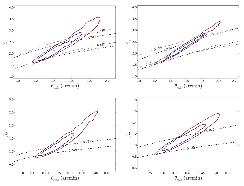
Figure 3: Confidence interval contours for the double $\beta$-model fit to the X-ray data of the MS 1054-0321 cluster, superposed with contours of the values of the gas mass fractions from the X-ray and SZ effect data. The best fit of the parameters are marked as crosses, while the blue and red solid contours correspond, respectively, the $68\%$ and $90\%$ confidence intervals. The dashed and dotted contours define, respectively, the gas mass fractions derived from the X-ray and SZ effect data.Upper and lower panels represent the confidence level contours of the shape parameters for the eastern and western components, respectively.

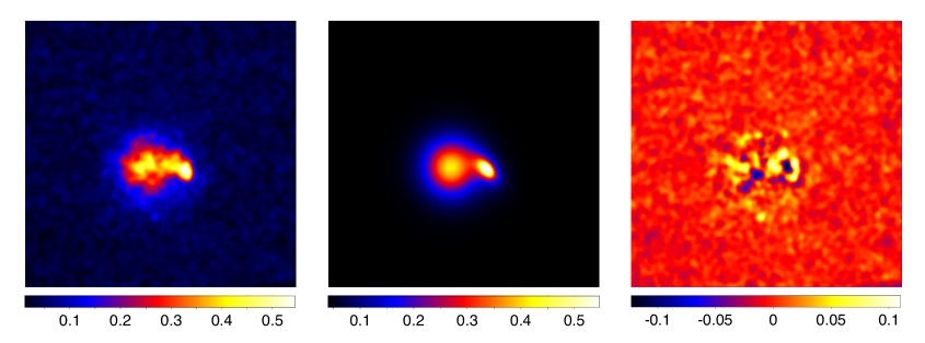
Figure 4: Left: Chandra X-ray image of the cluster MS 1054-0321 in the 0.5-7.0 keV band. Centre: the source model, made up of two elliptical $\beta$ models. Right: the residual image from the best-fit model. The colour scales at the bottom of each image are in units of counts pixel^-1, where a pixel has side $0.492\arcsec$.

5.2 Gas mass fraction

The gas mass fraction, $f_{gas}$, can be computed by dividing the gas mass by the total mass of the cluster. To determine the cluster masses as discussed in section 4.2, we need to define a limiting radius within which the masses are measured. Due to significant AGN activity in MS 1054-0321 relative to lower redshift clusters, particularly at distances between 1 and 2 Mpc (Best et al., 2002; Johnson, Best & Almaini, 2003), we carried out our measurements within the relatively small angular radius $\theta_{2500}$, corresponding to a density 2500 times the critical density of the Universe at the redshift of the cluster. The $\theta_{2500}$ radius of each cluster component can be obtained from

$$M_{tot}(\theta_{2500})=D_{A}^{3}\theta_{2500}^{3}\Delta\rho_{c}(z),$$ (12)

where the left-hand side is the total mass within angular radius ($\theta_{2500}$) given by equation (10), $\rho_{c}(z)$ is the critical density of the Universe, and $\Delta=2500$.

In Table 5, we show the gas and total masses, and the gas mass fractions, of the eastern and western components using the best fit parameters from our models with $\delta=0$. The 68$\%$ confidence interval errors associated with these are given for variations of the fitting parameters. For both models, the gas mass fractions derived from the X-ray and SZ effect data for the eastern component are consistent. It can be seen from the double $\beta$-model analysis that the X-ray gas mass fraction of the western component within $\theta_{2500}$ is about one third of that derived for the eastern component.

Table 5: The physical properties of the MS 1054-0321 cluster.

Single $\beta$-model
Region	$\theta_{2500}$	$M_{gas}^{\mathrm{X\mbox{-}ray}}$	$M_{gas}^{\mathrm{SZ}}$	$M_{tot}$	$f_{gas}^{\mathrm{X\mbox{-}ray}}$	$f_{gas}^{\mathrm{SZ}}$
	(arcsec)	$(10^{13}\,h_{100}^{-1}\,\mathrm{M_{\odot}})$	$(10^{13}\,h_{100}^{-1}\,\mathrm{M_{\odot}})$	$(10^{14}\,h_{100}^{-1}\,\mathrm{M_{\odot}})$
Eastern component	$40.9_{-1.0}^{+0.3}$	$1.30_{-0.01}^{+0.02}$	$1.33_{-0.01}^{+0.04}$	$1.45_{-0.02}^{+0.01}$	$0.090_{-0.001}^{+0.001}$	$0.092_{-0.001}^{+0.001}$
Double $\beta$-model
Eastern component	$44.8_{-1.0}^{+3.5}$	$1.67_{-0.01}^{+0.06}$	$1.79_{-0.05}^{+0.06}$	$1.91_{-0.11}^{+0.01}$	$0.087_{-0.001}^{+0.005}$	$0.094_{-0.001}^{+0.003}$
Western component	$43.9_{-4.9}^{+10.5}$	$0.53_{-0.12}^{+0.04}$	—	$1.79_{-0.36}^{+0.82}$	$0.030_{-0.014}^{+0.010}$	—

Although the values of the shape parameters extracted from the models are significantly different, we find that the gas and total masses, and thus the gas mass fraction, for the eastern component obtained from the single $\beta$-model are consistent with those derived from the double $\beta$-model over the same angular radius. The X-ray and SZ effect gas mass fractions from both models are in good agreement with those derived from a nonisothermal double $\beta$-model within $\theta_{2500}$ (LaRoque et al., 2006), and $\sim 70\%$ higher than that derived by Grego et al. (2001) within a larger angular radius. However, our gas mass fractions are $\sim 40\%$ lower than those derived from an isothermal $\beta$-model fit that excluded the central region from the X-ray data (LaRoque et al., 2006).

To compare our results with those derived by Bonamente et al. (2008), we estimate the gas and total masses within their angular radius $\theta=89\arcsec$. Within this radius, the derived X-ray and SZ effect gas masses for the eastern component from the single $\beta$-model analysis are, respectively, $4.40_{-0.01}^{+0.02}\times 10^{13}\,h_{100}^{-1}\,\mathrm{M_{\odot}}$ and $4.51_{-0.01}^{+0.06}\times 10^{13}\,h_{100}^{-1}\,\mathrm{M_{\odot}}$. From the double $\beta$-model fit, these gas masses are $4.36_{-0.04}^{+0.20}\times 10^{13}\,h_{100}^{-1}\,\mathrm{M_{\odot}}$ and $4.67_{-0.08}^{+0.16}\times 10^{13}\,h_{100}^{-1}\,\mathrm{M_{\odot}}$. These values are consistent with each other and with the gas mass of $5.18_{-0.70}^{+0.84}\times 10^{13}\,h_{100}^{-1}\,\mathrm{M_{\odot}}$ derived by Bonamente et al. (2008) within the same angular radius from an isothermal $\beta$-model fit to the X-ray data (excluding the central region) and to SZ effect data. Using the temperature of the eastern component, $10.7_{-1.5}^{+1.9}\,\mathrm{keV}$, our estimates of the total mass inside 89$\arcsec$ from the single and double $\beta$-models are $5.64_{-0.43}^{+0.68}\times 10^{14}\,h_{100}^{-1}\,\mathrm{M_{\odot}}$ and $7.70_{-1.00}^{+0.91}\times 10^{14}\,h_{100}^{-1}\,\mathrm{M_{\odot}}$, respectively. Such masses are $\sim 60\%$ larger than the mass of $3.15_{-0.70}^{+0.98}\times 10^{14}\,h_{100}^{-1}\,\mathrm{M_{\odot}}$ given by Bonamente et al. (2008). The estimated total masses fall to $4.48_{-0.34}^{+0.54}\times 10^{14}\,h_{100}^{-1}\,\mathrm{M_{\odot}}$ and $6.12_{-0.80}^{+0.73}\times 10^{14}\,h_{100}^{-1}\,\mathrm{M_{\odot}}$ from the single and double $\beta$-models if we adopt the lower temperature of $8.5\pm 0.7\,\mathrm{keV}$ measured for the total cluster. The former value is more consistent with that reported by Bonamente et al. (2008) than the total mass derived from the double $\beta$-model. The high total mass that we derived from the double $\beta$-model, relative to that derived from the single $\beta$-model, might suggest that the total mass is overestimated as a result of overlaps between the two components. The gas mass fractions obtained within $89\arcsec$ for the eastern component are $f_{gas}^{\mathrm{X\mbox{-}ray}}=0.102_{-0.011}^{+0.009}$ and $f_{gas}^{\mathrm{SZ}}=0.127_{-0.013}^{+0.010}$ from the single $\beta$-model analysis, and $f_{gas}^{\mathrm{X\mbox{-}ray}}=0.074_{-0.006}^{+0.015}$ and $f_{gas}^{\mathrm{SZ}}=0.096_{-0.007}^{+0.017}$ from the double $\beta$-model analysis. The average value of these gas mass fractions is $0.100_{-0.009}^{+0.013}$, about $40\%$ lower than the gas mass fraction estimated by Bonamente et al. (2008).

For the eastern component, the estimated X-ray and SZ gas mass fractions within $\theta_{2500}$ using the 1 Mpc offset parameters are consistent with those estimated using the 3 Mpc offset parameters, and only about $5\%$ higher than those derived at $\delta=0$. These results imply an systematic error of $\sim 0.002$ in the X-ray and SZ gas mass fractions due to uncertainty in the value of $\delta$. The X-ray gas mass fractions for the western component derived within $\theta_{2500}$ for 1 and 3 Mpc offsets agree, but are about $10\%$ higher than the value for $\delta=0$, suggesting an systematic error of $\sim 0.001$ in the gas mass fraction. These results indicate that the offset issue is not responsible for the low gas mass fraction in the eastern and western components.

The gas mass fraction of the eastern and western components together, within angular radius $\theta_{2500}$, is $0.060_{-0.009}^{+0.004}$. This fraction is small, and about two thirds of the gas mass fraction deduced from the eastern component. However, the value is in agreement with that reported by Grego et al. (2001) within $\theta_{500}$, and $\sim 40\%$ lower than the X-ray and SZ effect gas mass fractions measured from the nonisothermal double $\beta$-model (LaRoque et al., 2006).

To examine the effect of the isothermal assumption on the gas mass fraction measurements, we estimated the gas and total masses for both cluster components in the presence of the maximum temperature gradient (Section 3.2). For the eastern component, the estimated X-ray and SZ gas masses are higher by about $3\%$ and $20\%$ than those derived under the isothermal assumption, respectively. The total mass could be as much as $50\%$ lower than that derived from the isothermal assumption. The upper limits on the gas mass fractions are $\sim 0.140$ from the X-ray data, and $\sim 0.180$ from the SZ effect data. The estimated X-ray and SZ gas mass fractions therefore are $f_{gas}^{\mathrm{X\mbox{-}ray}}=0.087_{-0.001}^{+0.005}\,\rm{(random)}\,{}_{-0.001}^{+0.053}\,\rm{(systematic)}$ and $f_{gas}^{\mathrm{SZ}}=0.094_{-0.001}^{+0.003}\,\rm{(random)}\,{}_{-0.001}^{+0.086}\,\rm{(systematic)}$. For the western component, the X-ray gas mass fraction is affected by less than $10\%$ by the isothermal assumption. Thus the gas mass fraction in the eastern component could approach the cosmic value, while the western component is gas-poor. Any contribution from the non-thermal pressure would tend to reinforce our conclusion of low gas mass fraction.

Such a low gas mass fraction could suggest that the gas content of the cluster, particularly the western component, is being stripped. This scenario was also proposed by Jeltema et al. (2001). Gas stripping in this cluster is likely since it contains a large fraction of merging galaxies (17$\%$, van Dokkum et al., 2000), which might indicate that MS 1054-0321 has not yet reached a steady state. Accordingly, measurements of the component gas mass fractions under the assumptions of isothermal and hydrodynamic equilibrium conditions could be questionable. The stronger dependence of the SZ gas mass on temperature suggest that a sensitive SZ map extending to larger radii from the cluster centre might reveal the missing gas mass if the outer gas is relatively cool.

6 Summary

Using archival Chandra data, we have re-analysed the temperature structure of the MS 1054-0321 cluster. The best fit model to the cluster X-ray spectrum within $90\arcsec$ of the cluster centre gives X-ray temperature $T=8.5\pm 0.7\,\mathrm{keV}$ and iron abundance $Z=0.33\pm 0.11\,\mathrm{Z_{\odot}}$. The measured temperature is consistent with the Chandra temperature reported by Jee et al. (2005) and Tozzi et al. (2003), and also with the XMM–Newton temperature (Gioia et al., 2004). However, this temperature is lower by $\sim 18\%$ than the Chandra temperature derived by Jeltema et al. (2001), and by $30\%$ than the ASCA temperature (Donahue et al., 1998). The iron abundance is in agreement with the values reported by Gioia et al. (2004) and Jee et al. (2005). The temperature of the eastern component of MS 1054-0321 is significantly higher than that of the western component (Section 3.2). Such a temperature difference is consistent with previous work (Jeltema et al., 2001; Gioia et al., 2004; Jee et al., 2005).

We have measured the central SZ effect signal at 30 GHz towards MS 1054-0321 with OCRA-p. The contaminated SZ effect signal towards the cluster centre is $-2.18\pm 0.33\,\mathrm{mJy}$. The radio environment within an angular radius of 4.5 arcmin of the cluster centre was investigated, and used to form a source-corrected SZ effect of $-2.55\pm 0.33\,\mathrm{mJy}$.

We have investigated the gas mass distribution of the MS 1054-0321 cluster using triaxial $\beta$-type models. In addition to fitting the X-ray data of the eastern component with a single triaxial $\beta$-model, we have fitted the X-ray image of the entire cluster to a double triaxial $\beta$-model, which gives a significantly better description of the gas structure of the cluster. For the single and double $\beta$-models, the gas mass fractions estimated from the X-ray and SZ effect data for the eastern component are in good agreement. Using different offsets along the line of sight, results obtained from the double $\beta$-model suggest that the gas mass fraction of the western component is about three times lower than those of the eastern component.

Despite a significant variation in the shape parameters for the models, the X-ray and SZ gas mass fractions for the eastern component derived from the single $\beta$-model are consistent with those derived from the double $\beta$-model within the same region. For both models, the gas mass fractions are in good agreement with those derived from a nonisothermal $\beta$-model (LaRoque et al., 2006), and higher than the gas mass fraction reported by Grego et al. (2001) over the larger region. The X-ray and SZ gas mass within angular radius $89\arcsec$ from both models agree well with those reported by Bonamente et al. (2008). Using the integrated X-ray temperature of the cluster, the average gas mass fraction estimated for the eastern component at $\delta=0$ is $0.100_{-0.009}^{+0.013}$, about $40\%$ lower than that reported by Bonamente et al. (2008). The gas mass fraction of the overall cluster, within $\theta_{2500}$, is $0.060_{-0.009}^{+0.004}$. This is in agreement with the gas mass fraction reported by Grego et al. (2001). The relative model-independence of these gas mass fractions suggests that these estimates are robust and reliable.

We have quantified the effect of the isothermal assumption and hydrostatic equilibrium condition on measurements of the gas and total masses, and thus the gas mass fraction of the cluster. For the eastern component, the X-ray and SZ gas mass fractions could rise to $\sim 0.140$ and $\sim 0.180$, respectively. For the western component, the X-ray gas mass fraction is less affected by the isothermal assumption. Contributions from non-thermal pressure could lower the estimated gas content of this component even further.

We suggest that the low gas mass fraction of the cluster, particularly in the western component, could be a result of gas stripping. This scenario is consistent with the merger picture of the cluster (van Dokkum et al., 2000), and the assumptions of the isothermal and hydrostatic equilibrium conditions are therefore questionable. Observations with better signal/noise in the SZ effect could reveal more about the nature of this cluster and locate the missing baryons, and significantly deeper Chandra observations could resolve uncertainties about the temperature structure of the eastern component.

References

- Anders & Grevesse (1989) Anders E., Grevesse N., 1989, Geochim. Cosmochim. Acta, 53, 197
- Battaglia et al. (2012) Battaglia N., Bond J. R., Pfrommer C., Sievers J. L., 2012, ApJ, 758, 75
- Best et al. (2002) Best P. N., van Dokkum P. G., Franx M., Röttgering H. J. A., 2002, MNRAS, 330, 17
- Birkinshaw (1999) Birkinshaw M., 1999, Phys. Rep., 310, 97
- Birkinshaw & Lancaster (2008) Birkinshaw M., Lancaster K., 2008, Lect. Notes Phys., 740, 255
- Birkinshaw, Hughes & Arnaud (1991) Birkinshaw M., Hughes J. P., Arnaud K. A., 1991, ApJ, 379, 466
- Bonamente et al. (2006) Bonamente M., Joy M. K., LaRoque S. J., Carlstrom J. E., Reese E. D., Dawson K. S., 2006, ApJ, 647, 25
- Bonamente et al. (2008) Bonamente M., Joy M., LaRoque S. J., Carlstrom J. E., Nagai D., Marrone D. P., 2008, ApJ, 675, 106
- Brodwin et al. (2012) Brodwin M. et al., 2012, ApJ, 753, 162
- Carlstrom, Holder & Reese (2002) Carlstrom J. E., Holder G. P., Reese E. D., 2002, ARA&A, 40, 643
- Carlstrom et al. (2011) Carlstrom J. E. et al., 2011, PASP, 123, 568
- Coble et al. (2007) Coble K. et al., 2007, 134, 897
- Condon et al. (1998) Condon J. J., Cotton W. D., Greisen E. W., Yin Q. F., Perley R. A., Taylor G. B., Broderick J. J., 1998, AJ, 115, 1693
- Dickey & Lockman (1990) Dickey J. N., Lockman F. J., 1990, ARA&A, 28, 215
- Donahue et al. (1998) Donahue M., Voit G. M., Gioia I. M., Luppino G., Hughes J. P., Stocke J. T., 1998, ApJ, 502, 550
- Evrard, Metzler & Navarro (1996) Evrard A. E., Metzler C. A., Navarro J. F., 1996, ApJ, 469, 494
- Fixsen (2009) Fixsen D. J., 2009, ApJ, 707, 916
- Foley et al. (2011) Foley R. J. et al., 2011, ApJ, 731, 86
- Gioia et al. (1990) Gioia I. M., Maccacaro T., Schild R. E., Wolter A., Stocke J. T., Morris S. L., Henry J. P., 1990, ApJS, 72, 567
- Gioia et al. (2004) Gioia I. M., Braito V., Branchesi M., Della Ceca R., Maccacaro T., Tran K.-V., 2004,A&A, 419, 517
- Grego et al. (2001) Grego L., Carlstrom J. E., Reese E. D., Holder G. P., Holzapfel W. L., Joy M. K., Mohr J. J., Patel S., 2001, ApJ, 552, 2
- Hoekstra, Franx & Kuijken (2000) Hoekstra H., Franx M., Kuijken K., 2000, ApJ, 532, 88
- Jee et al. (2005) Jee M. J., White R. L., Ford H. C., Blakeslee J. P., Illingworth G. D., Coe D. A., Tran K.-V. H., 2005, ApJ, 634, 813
- Jeltema et al. (2001) Jeltema T. E., Canizares C. R., Bautz M. W., Malm M. R., Donahue M., Garmire G. P., 2001, ApJ, 562, 124
- Johnson, Best & Almaini (2003) Johnson O., Best P. N., Almaini O., 2003, MNRAS, 343, 924
- Joy et al. (2001) Joy M. et al., 2001, ApJ, 551, L1
- Lancaster et al. (2007) Lancaster K. et al., 2007, MNRAS, 378, 673
- Lancaster et al. (2011) Lancaster K. et al., 2011, MNRAS, 418, 1441
- LaRoque et al. (2006) LaRoque S. J., Bonamente M., Carlstrom J. E., Joy M. K., Nagai D., Reese E. D., Dawson K. S., 2006, ApJ, 652, 917
- Luppino & Kaiser (1997) Luppino G. A., Kaiser N., 1997, ApJ, 475, 20
- Medezinski et al. (2011) Medezinski E., Broadhurst T., Umetsu K., Benítez N., Taylor A., 2011, MNRAS, 414, 1840
- Mewe, Gronenschild & van den Oord (1985) Mewe R., Gronenschild E. H. B. M., van den Oord G. H. J., 1985, A&AS, 62, 197
- Morandi, Ettori & Moscardini (2007) Morandi A., Ettori S., Moscardini L., 2007, MNRAS, 379, 518
- Neumann & Arnaud (2000) Neumann D. M., Arnaud M., 2000, ApJ, 542, 35
- Planck Collaboration (2013) Planck Collaboration V., 2013, A&A, 550, A131
- Pratt et al. (2009) Pratt G. W., Croston J. H., Arnaud M., Böhringer H., 2009, A&A, 498, 361
- Rephaeli (1995) Rephaeli Y., 1995, ARA&A, 33, 541
- Tozzi et al. (2003) Tozzi P., Rosati P., Ettori S., Borgani S., Mainieri V., Norman C., 2003, ApJ, 593, 705
- van Dokkum et al. (2000) van Dokkum P. G., Franx M., Fabricant D., Illingworth G. D., Kelson D. D., 2000, ApJ, 541, 95
- Vikhlinin et al. (2006) Vikhlinin A., Kravtsov A., Forman W., Jones C., Markevitch M., Murray S. S., Van Speybroeck L., 2006, ApJ, 640, 691
- Wen & Han (2011) Wen Z. L., Han J. L., 2011, ApJ, 734, 68
- Worrall & Birkinshaw (2003) Worrall D. M., Birkinshaw M., 2003, MNRAS, 340, 1261
- Zaritsky & Gonzalez (2003) Zaritsky D., Gonzalez A. H., 2003, ApJ, 584, 691