Role of natural convection in the dissolution of sessile droplets

Abstract

The dissolution process of small (initial (equivalent) radius $R_{0}<1$ mm) long-chain alcohol (of various types) sessile droplets in water is studied, disentangling diffusive and convective contributions. The latter can arise for high solubilities of the alcohol, as the density of the alcohol-water mixture is then considerably less as that of pure water, giving rise to buoyancy driven convection. The convective flow around the droplets is measured, using micro-particle image velocimetry ($\mathrm{\SIUnitSymbolMicro}$PIV) and the schlieren technique. When non-dimensionalizing the system, we find a universal $\text{Sh}\sim\text{Ra}^{1/4}$ scaling relation for all alcohols (of different solubilities) and all droplets in the convective regime. Here Sh is the Sherwood number (dimensionless mass flux) and Ra the Rayleigh number (dimensionless density difference between clean and alcohol-saturated water). This scaling implies the scaling relation $\tau_{\text{c}}\propto R_{0}^{5/4}$ of the convective dissolution time $\tau_{\text{c}}$, which is found to agree with experimental data. We show that in the convective regime the plume Reynolds number (the dimensionless velocity) of the detaching alcohol-saturated plume follows $\text{Re}_{\text{p}}\sim\text{Sc}^{-1}\text{Ra}^{5/8}$, which is confirmed by the $\mathrm{\SIUnitSymbolMicro}$PIV data. Here, Sc is the Schmidt number. The convective regime exists when $\text{Ra}>\text{Ra}_{\text{t}}$, where $\text{Ra}_{\text{t}}=12$ is the transition Ra-number as extracted from the data. For $\text{Ra}\leq\text{Ra}_{\text{t}}$ and smaller, convective transport is progressively overtaken by diffusion and the above scaling relations break down.

1 Introduction

Conventional wisdom says that oil and water do not mix. However, some oily liquids, e.g. long-chain alcohols, are slightly soluble in water (see table 1). When a droplet of such an alcohol is placed in a bath of water, it will slowly dissolve. Figure 1 shows an example of a sessile 1-hexanol droplet in water for which the dissolution time $\tau$ was about 3 hours. Considering this long dissolution time, it may seem plausible to assume that mass transport away from the droplet is governed by diffusion. Equivalent to the diffusion driven mass transport from small gas bubbles (Epstein & Plesset, 1950) or small sessile droplets (Popov, 2005; Stauber et al., 2014; Zhang et al., 2015; Lohse & Zhang, 2015) the relevant time-scale would in this case then be given by

$$\tau_{\text{d}}=\frac{R_{0}^{2}\rho_{\text{d}}}{2D\Delta c}$$ (1)

where $R_{0}$ is the initial equivalent radius of the droplet, $D$ the diffusion constant of the alcohol in water, $\rho_{\text{d}}$ is the density of the droplet material, and $\Delta c$ is the difference between the saturated concentration $c_{s}$ at the droplet interface and the (undersaturated) concentration $c_{\infty}<c_{s}$ far away from the drop. However, for the 1-hexanol droplet with an initial radius $R_{0}=0.7$ mm, one finds $\tau_{\text{d}}\approx 11$ hours, which is much longer than the 3 hours observed experimentally. In previous work (Dietrich et al., 2015) we hypothesized that this discrepancy is caused by the neglect of buoyancy driven convection of the slightly lighter alcohol-water mixture near the droplet interface. The same idea has been put forward in the context of slowly growing CO₂ bubbles in small supersaturations (Enríquez et al., 2014; Peñas López et al., 2015), and evaporating droplets (Shahidzadeh-Bonn et al., 2006). Also in these cases, the rate of mass transport exceeded the diffusion limited predictions. On the other hand, even for mm-sized droplets, there also seem to be circumstances under which the diffusive time scale is accurate (Picknett & Bexon, 1977; Gelderblom et al., 2011; Stauber et al., 2014, 2015b). This reflects the existence of a threshold for convection. However, the details of this threshold remain unclear. The low velocities and small refractive index differences involved often inhibit direct observation of the buoyant flow in the surrounding medium. As far as we are aware, direct visualization attempts of the external flow were only undertaken in the context of evaporating droplets, using either schlieren (Kelly-Zion et al., 2013b), infrared spectroscopy (Kelly-Zion et al., 2013a), interferometry (Dehaeck et al., 2014), and only very recently, by tracing tiny oil droplets in air (Somasundaram et al., 2015).

In this work we combine qualitative schlieren imaging with quantitative micro-particle image velocimetry ($\mathrm{\SIUnitSymbolMicro}$PIV) to directly visualize the concentration field and flow around slowly dissolving droplets of various types of long-chain alcohols in clean water. We show that above a transition solutal Rayleigh number, which corresponds to the buoyancy of the alcohol-water mixture, which is lighter than the surrounding clean water, the solute is mainly transported away in a single steady plume above the droplet. Knowledge of the flow structure allows us to derive scaling laws for both the dissolution rate and the plume velocity in the convective regime, which are in good agreement with experiments. Finally, as the droplet shrinks and its Rayleigh number drops below the transition value, a transition occurs in which convection dies out and is overtaken by diffusion.

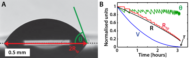
Figure 1: (A) Snapshot of a dissolving long-chain alcohol droplet (1-hexanol) in water. The dotted black line indicates the location of the silicon substrate, which mirrors part of the droplet. The footprint radius $R_{\rm{\rm{fp}}}$ and the contact angle $\theta$ are indicated. A movie of the entire dissolution process is available online as supplementary material. (B) Evolution of the aforementioned parameters in time, along with the volume $V$ of the droplet and the equivalent radius $R=\left(3V/2\pi\right)^{1/3}$. All parameters have been normalised by their initial values: $V_{0}=750$ nL, $R_{\rm{fp},0}=0.825$ $\mathrm{mm}$, $R_{0}=0.708$ $\mathrm{mm}$, and $\theta_{0}=72^{\circ}$.

2 Experimental Procedure

2.1 Materials and Preparation

As shown in table 1 the solubility of long-chain alcohols strongly depends on their length, while other properties, like density and diffusion coefficient are relatively insensitive to this. By increasing the number of carbon atoms in the chain from 5 (pentanol) to 8 (octanol), one decreases the solubility (and thereby the buoyant force of the water-alcohol mixture) by two orders of magnitude. This makes these alcohols very suitable to study the possible transition between diffusion and convection. Alcohols with purities of $\geq 98\%$ (Sigma-Aldrich) were used. The density of the alcohol-water mixture (table 1) was calculated for a mixture at $100\%$ saturation, using the molal volume $\phi_{V}^{0}$ at infinite dilution (Høiland & Vikingstad, 1976; Romero et al., 2007). The molal volume $\phi_{V}$ gives the volume occupied by one mole of solute in the solvent. The assumption is made that $\phi_{V}$ is independent of the solute concentration, which introduces a negligible error in $\Delta\rho$ of $<1\%$ when compared to the direct density measurements given by Romero et al. (2007).

Table 1: Properties of the alcohols used in this work, measured at $25^{\circ}$C: Chemical composition, density $\rho$ of the pure alcohol, diffusion constant $D$ of the alcohol in water, saturation solubility $c_{s}$ of the alcohol in water, molal volume $\phi_{V}^{0}$ of the alcohol in water at infinite dilution, density difference $\Delta\rho=\rho_{H_{2}O}-\rho_{H_{2}O,\text{sat}}$ between clean water and water saturated with the alcohol, interfacial tension $\gamma$ of the water-alcohol interface. The diffusive timescale $\tau_{\text{d}}$ is calculated according to equation (1), for $R_{0}=0.7$ mm. No values for $\gamma$ for 2-heptanol and 3-heptanol could be found. Data were obtained from Crittenden & Hixson (1954)^‡, Kinoshita et al. (1958)^∗, Høiland & Vikingstad (1976)^♠, Stephenson et al. (1984)^♭, Demond & Lindner (1993)^♣, Hao & Leaist (1996)^†, Romero et al. (2007)^⋆, and Yalkowsky et al. (2010)^◆. Diffusion constants for 2-heptanol and 3-heptanol were assumed to be equal to the 1-heptanol value, and the diffusion constant of 1-octanol was obtained by extrapolating data from Hao & Leaist (1996).

Alcohol	Composition	$\rho$	D	$c_{s}$	$\phi_{V}^{0}$	$\Delta\rho$	$\gamma$	$\tau_{\text{d}}$
		[kg m-3]	[$10^{-9}$m2s-1]	[kg m-3]	[cm3mol-1]	[kg m-3]	[mN/m]	[$10^{4}$ s]
1-Pentanol	C5H11OH	$811$	$0.888^{\dagger}$	$22^{\ddagger\ast}$	$102.62^{\star\spadesuit}$	$3.42$	$4.4^{\clubsuit}$	$1.0$
1-Hexanol	C6H13OH	$814$	$0.83^{\dagger}$	$5.9^{\ddagger\ast}$	$118.65^{\star\spadesuit}$	$0.92$	$6.8^{\clubsuit}$	$4.0$
1-Heptanol	C7H15OH	$822$	$0.800^{\dagger}$	$1.67^{\ast}$	$136.95^{\star}$	$0.29$	$7.7^{\clubsuit}$	$14.5$
2-Heptanol	C7H15OH	$817$	$0.800$	$3.5^{\flat}$	$134.39^{\spadesuit}$	$0.53$	-	$7.6$
3-Heptanol	C7H15OH	$818$	$0.800$	$4.0^{\ddagger\blacklozenge}$	$133.30^{\spadesuit}$	$0.57$	-	$5.8$
1-Octanol	C8H17OH	$827$	$0.780$	$0.5^{\ddagger\ast}$	$148.41^{\star}$	$0.07$	$8.52^{\clubsuit}$	$48.1$

A sketch of the experimental setup is provided in figure 2. All measurements were conducted in a qubic glass tank of $5\times 5\times 5$ cm³. The container was cleaned using isopropyl-alcohol and water, and then filled with $100$ $\mathrm{ml}$ of clean water. This water was obtained from a Reference A+ system (Merck Millipore, at $18.2$ $\mathrm{M\SIUnitSymbolOhm}\text{\,}\mathrm{cm}$) several hours before the measurement and stored in a clean flask to equilibrate and thus reduce thermal convective currents. After the tank was filled, a single droplet was dispensed from a glass syringe with a teflon plunger, fitted in a motorized syringe pump. The droplet was placed on a hydrophobized silicon wafer $\approx 1\times 1$ cm² (P/Boron/(100), Okmetic), placed at the bottom of the tank. Hydrophobization was achieved by coating the wafer with a self-assembled monolayer of PFDTS (1H,1H,2H,2H-Perfluorodecyltrichlorosilane 97%, ABCR Gmbh, Karlsruhe Germany), following the procedure described earlier (Karpitschka, 2012). Prior to each experiment the samples were cleaned by insonication in acetone for $10$ $\mathrm{min}$ and dried under a stream of nitrogen. After the droplet was placed on the substrate, the needle was removed and the tank was closed.

2.2 Imaging

The droplet was illuminated from one side using a collimated LED light source (Thorlabs, wavelength $\lambda=625$ nm) and imaged onto a CCD camera (Pixelfly USB, PCO Germany) with a long-distance microscope providing a magnification up to $16\times$. The images were recorded at a rate of 1 frame per second, and post-processed using a Matlab code to extract the droplet profile with sub-pixel accuracy (van der Bos et al., 2014). Since all droplets were smaller than the capillary length ($\sqrt{\gamma/(\rho_{H_{2}O}-\rho_{alcohol})g}\approx 2$ mm), the droplet profile could accurately be fitted to a spherical cap to obtain the radius of curvature and contact angle. With this method, droplets could be traced until $V<0.05V_{0}$.

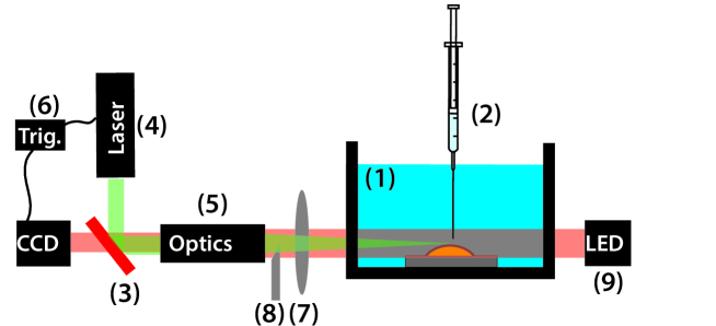
Figure 2: (color online) Experimental setup, showing the glass tank (1), with the substrate and the droplet in place (not to scale). The droplet was deposited under water using a syringe (2) fitted in a motorized syringe pump (not drawn). A dichroic mirror (3) was used to couple the laser beam (4) into the long distance microscope (5). A trigger-delay box (6) synchronized the laser pulses with the camera exposure. Parts (3), (4), and (6) were used in the $\mathrm{\SIUnitSymbolMicro}$PIV measurements only. The assembly used for schlieren, consisting of a positive lens (7) and a knife edge (8) located in the focal point of the lens. The parallel LED light source (9) was used in all experiments, with the exception of the PIV measurements.

2.3 Schlieren

The concentration gradients developing around the dissolving droplets were qualitatively visualized using the schlieren technique (Settles, 2001). For this, a positive lens and a knife edge were placed at the camera side of the tank, as shown in figure 2. After passing through the tank, the parallel light from the LED source is focused onto the edge of a sharp knife placed perpendicular to the beam. To be sensitive to both horizontal and vertical concentration gradients the knife edge was placed under an angle of $45^{\circ}$. In the resulting image, solute rich regions are visible as a local changes in light intensity.

2.4 $\mu$PIV measurements

For the $\mathrm{\SIUnitSymbolMicro}$PIV measurements the water in the tank was seeded with red-fluorescent tracer particles (Fluoro-Max, Thermo Fisher Scientific, $3$ $\mathrm{\SIUnitSymbolMicro m}$ diameter). A pulsed green laser, (Nd:YAG, $\lambda=532$ nm) was coupled into the microscope by a dichroic mirror. The focal plane of the microscope was centered at the droplet. Therefore, only tracer particles in the $\approx 100$ $\mathrm{\SIUnitSymbolMicro m}$ thick focal plane were imaged, producing a 2-dimensional velocity field around the symmetry axis of the droplet. The red light ($\lambda=612$ $\mathrm{nm}$) emitted by the fluorescent particles was recorded by the CCD camera at $8$ frames per second. A BNC 575 pulse/delay generator was used to synchronize the laser pulse and the camera exposure. The obtained images were then post-processed in ImageJ to remove static features and to enhance the contrast. Consecutive image pairs were analyzed with JPIV, using an interrogation window of $32\times 32$ pixels, corresponding to $\approx 70\times 70$ ${\mathrm{\SIUnitSymbolMicro m}}^{2}$. The concentration of tracer particles was kept low to avoid excessive absorption and blurring by out of focus particles. Because of this low particle density, the velocity fields from multiple images pairs were combined for improved accuracy (Raffel et al., 2007).

3 Visualization results

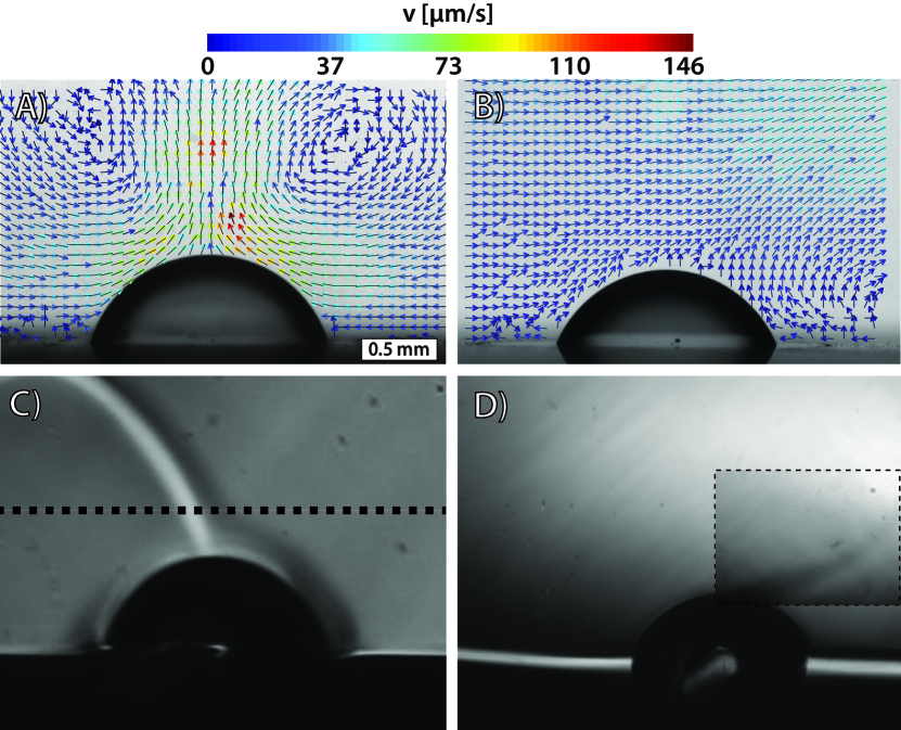
Figure 3: (color online) Velocity fields (A&B) and solute concentration fields (C&D) surrounding droplets dissolving in water. A&C show droplets of 1-pentanol, B&D droplets of 1-heptanol. The contrast of the outlined area in D has been modified to increase the visibility of the plume. Note that panels A-C and B-D represent separate experiments. The dashed line in C indicates where the cross-sectional profiles, shown in figure 5, are taken. The images were taken approximately 30 seconds (A), 2 minutes (C) or 4 minutes (B&D) after deposition of the droplet.

Figure 3 shows snapshots of the $\mathrm{\SIUnitSymbolMicro}$PIV and schlieren measurements for 1-pentanol (left) and 1-heptanol droplets (right). The dissolving 1-pentanol droplet generates a clear plume originating from its apex, while fresh liquid is drawn in from the sides. The tip of the plume ends in a vortex ring which moves away from the droplet as the experiment proceeds, leaving behind a single plume (see figure 3C). For 1-heptanol, with its lower solubility, the plume is far less pronounced. The particle velocities are significantly lower and the contrast of the schlieren image had to be strongly enhanced to see the plume at all (see figure 3D). The weak 1-heptanol plume seems to be affected by a small mean flow in the cell, possibly caused by thermal convection due to changes in room temperature or the illumination. As we will show later on, this mean flow seems to have little influence on the dissolution behavior. Appendix A contains additional $\mathrm{\SIUnitSymbolMicro}$PIV results, including time-resolved velocity fields around a 1-pentanol droplet, the velocity field around an insoluble sessile droplet, and the flow around a dissolving sessile droplet placed on a vertical substrate. A movie, showing the motion of the bulk around the dissolving droplet, is available online as supplementary material.

The two different techniques used in figure 3 reveal that the convective plume displays two different features, as illustrated in figure 4. Firstly, the schlieren images visualize the plume shaped region that contains dissolved alcohol. The concentration profile is characterized by a width $2\delta_{c}$, which increases as $\delta_{c}\propto\sqrt{Dz/v_{p}}$, with $z$ the height above the droplet, and $v_{p}$ the plume flow speed. Secondly, the buoyant force on the (lighter) water-alcohol mixture results in a flow, as visualized by the $\mathrm{\SIUnitSymbolMicro}$PIV. The velocity profile of this flow (also drawn in figure 4) is characterized by a width $2\delta_{v}$. The liquid viscosity $\nu$ causes also the velocity profile to broaden for increasing height, namely with the same height dependence as the concentration profile, i.e. $\delta_{v}\sim\sqrt{\nu z/v_{p}}$. Therefore, the ratio $\zeta$ between the widths of the concentration and velocity profiles is fixed, $\zeta=\delta_{v}/\delta_{c}\sim\sqrt{\text{Sc}}$ (Bejan, 1993), where Sc is the Schmidt number $\text{Sc}\equiv\nu/D$. In the current system $\text{Sc}\approx 1200$, so $\delta_{v}\approx 30\delta_{c}$ is expected.

To obtain a theoretical description for the velocity and concentration profiles at Sc$=1200$, we solved equations (II.8) and (II.9), of the paper of Fujii (1963), who described the analogous case of a thermal plume above a heat source. Here, we followed the numerical procedure described by Vázquez et al. (1996), and used equation (II.15) from Fujii’s paper as a condition in the solving procedure, to obtain the velocity and concentration profiles at Sc$=1200$, as shown in figure 5A by the black and pink lines, respectively. The lateral coordinate $\tilde{X}$ in the theory is scaled by $\sqrt{Lz}$, with $L=\sqrt{2\pi\nu^{3}/(g\beta_{c}\dot{m}_{\text{d}})}$, where $g$ is the acceleration of gravity, $\beta_{c}\equiv\frac{\partial\rho}{\partial c}/\rho_{b}$ is the solutal expansion coefficient, and $\dot{m}_{\text{d}}$ is the mass loss rate of the droplet. The high Sc-number in the current system results in distinct shapes for the velocity and concentration profiles. The measured value for $\zeta$ therefore depends on the definition of the plume width, as shown in 5A. The anticipated $\zeta=30$ is retrieved when evaluated at a relative amplitude of $0.1$, corresponding to the $90\%$ boundary layer definition.

To compare our measurements to the theoretical profiles, a cross sectional intensity profile was measured in the schlieren image (figure 3C) at a height of $300$ $\mathrm{\SIUnitSymbolMicro m}$ above the apex of the droplet (as illustrated by the dashed line in figure 3C). This intensity profile is plotted as the solid red line in figure 5B, where we have to keep in mind that it represents the first derivative of the concentration profile, as it is the result from a schlieren measurement. To allow for an easy comparison, we plotted the theoretical concentration profile (pink solid line) from figure 5A and its derivative (red-dashed line) in figure 5B, and fitted the derivative to match the experiment. From this fit, a conversion factor was obtained to translate the dimensionless lateral coordinate of the theory to the length scale of the experiment. We executed the same procedure to obtain the velocity profile from the $\mathrm{\SIUnitSymbolMicro}$PIV data in figure 3A, again at $300$ $\mathrm{\SIUnitSymbolMicro m}$ above the droplet. This profile is plotted as the black circles in figure 5C. The theoretical velocity profile (black solid line) is superimposed on the measurement, where the previously found conversion factor was used to match the lateral coordinate. Comparison of the experimental and theoretical profiles in figure 5C reveals that while the central part of the plume shows fair agreement with the theoretical profile, the general shape of the plume is much narrower than expected from theory. The cause of this discrepancy is not understood as of yet. Possibly the vortex, substrate, and the droplet influence the plume shape, and the expected profile can be recovered when measured at higher distance above the droplet.

As mentioned before, the plume changes over time. To visualize the evolution of the plume, cross sections are taken in the $\mathrm{\SIUnitSymbolMicro}$PIV data at subsequent times, at $300$ $\mathrm{\SIUnitSymbolMicro m}$ above the 1-pentanol droplet. These cross sections are plotted in figure 5D, and show that the plume properties are linked to the droplet size: both the width and the maximum velocity of the plume steadily decrease as the droplet shrinks. At $t=3000$ s, the droplet has dissolved completely.

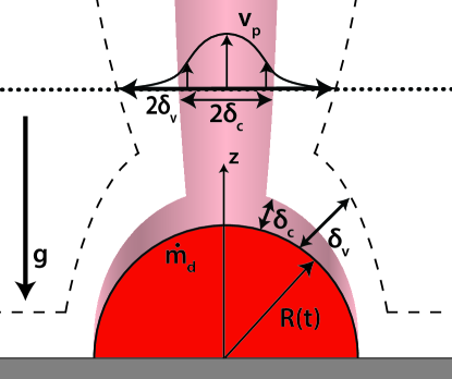
Figure 4: (color online) Sketch of a sessile droplet dissolving at a rate $\dot{m}_{\text{d}}$, and convective plume. A concentration boundary layer of thickness $\delta_{c}$ develops over the droplet interface, since $Sc\gg 1$, the velocity boundary layer has a thickness $\delta_{v}>\delta_{c}$. The boundary layers merge into plumes with diameters $2\delta_{c}$ and $2\delta_{v}$, moving at a vertical velocity $v_{p}$. The boundary layer widths $\delta_{c}$ and $\delta_{v}$ will change as a function of height, but are linked via the relation $\delta_{v}/\delta_{c}\sim\sqrt{\text{Sc}}$ (Bejan, 1993).

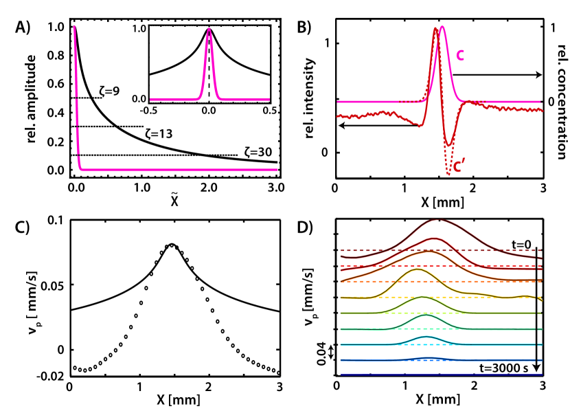
Figure 5: (color online) A) Theoretical velocity profile (black) and concentration profile (pink) for a plume at Sc$=1200$. The profiles are axi-symmetric around their plume centre at dimensionless lateral coordinate $\tilde{X}=0$, as illustrated in the inset, which shows a zoom around $\tilde{X}=0$. The observed ratio $\zeta=\delta_{v}/\delta_{c}$ depends on the definition of the plume width, as illustrated by the horizontal dashed lines. The anticipated $\zeta=30$ is recovered when the plume width is evaluated at a relative amplitude of $0.1$. B) The schlieren signal (red line), measured at a horizontal cross section $300$ $\mathrm{\SIUnitSymbolMicro m}$ above a 1-pentanol droplet ($R_{0}=700$ $\mathrm{\SIUnitSymbolMicro m}$), represents the derivative of the concentration profile. Therefore, both the theoretical concentration profile (pink solid curve) and its derivative (red-dashed curve) are plotted, and the derivative is fitted to match the schlieren measurement. Panel C shows the velocity profile (black circles), also measured at $300$ $\mathrm{\SIUnitSymbolMicro m}$ above an equally sized 1-pentanol droplet, and the theoretical velocity profile (black solid line). Panel D shows the velocity profiles at subsequent times, revealing that both the plume width and velocity decrease. For clarity, the plots are vertically shifted, with the baselines $v_{p}=0$ given as dashed lines. At $t=3000$ s, both droplet and plume have disappeared.

4 Dissolution rate and plume velocity

The $\mathrm{\SIUnitSymbolMicro}$PIV and schlieren images show that the convective flow around small droplets takes the form of a thin boundary layer over the droplet interface, culminating in a single plume rising from its apex. A schematic drawing of this flow and the concentration profile is shown in figure 4. If we assume (1) that at the interface of the droplet the solute concentration is constant and equal to $c_{s}$ and (2) that the droplet shrinks sufficiently slow. Then this situation is mathematically equivalent to the buoyant flow around a hot sphere of constant temperature $T$ and fixed radius $R$. In the context of thermal convection, the flow structure in both the boundary layer and plume are well known (see e.g. Bejan (1993), and Fujii (1963)). In this section we recapitulate the main findings in terms of the dissolution problem and compare them directly to our observations.

4.1 Dissolution rate

To study the droplet dissolution dynamics as a function of droplet liquid and size, individual droplets of varying initial volume and alcohol type were imaged throughout the dissolution process. Since the footprint radius $R_{\text{fp}}$ shows steps due to the stick-jump mode dissolution (Zhang et al., 2015; Dietrich et al., 2015; Lohse & Zhang, 2015), we define the equivalent radius $R\equiv\left(3V/(2\pi)\right)^{1/3}$ to provide a continuously decreasing measure for the droplet size. Figure 6 shows $R(t)$ for 1-pentanol (6A) and 1-heptanol (6B) droplets. From this, the mass loss rate $\dot{m}_{\text{d}}$ was extracted and plotted as a function of $R$ in figure 7 for all six alcohols. Note that while $\dot{m}<0$ for a shrinking droplet, we define the droplet mass loss rate as a positive amount, as it provides a more intuitive measure for the dissolution process. Using this, figure 7 shows that the measured mass loss rates for the various droplet sizes and alcohol types span two orders of magnitude. To find a universal description for the dissolution dynamics, we continue by defining dimensionless numbers which take both the droplet size and liquid into account.

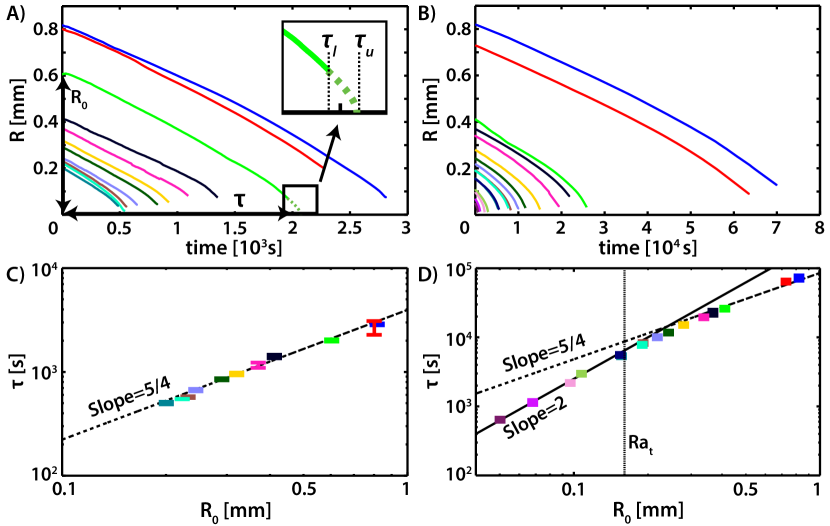
Figure 6: (color online) Equivalent radius $R=(3V/2\pi)^{1/3}$ as a function of time for 1-pentanol droplets (A) and 1-heptanol droplets (B) dissolving in water. The inset in A illustrates how for each droplet with initial radius $R_{0}$, the lifetime $\tau$ is estimated to lie between the lower estimate $\tau_{\text{l}}$ at the end of the experiment, and the upper estimate $\tau_{\text{u}}$, found by extrapolation using equation (13) (green dashed line). The lifetime $\tau$ is plotted as a function of $R_{0}$ in figures C and D for the 1-pentanol and 1-heptanol measurements, respectively. The lines in figures C and D illustrate the $\tau\sim{R}_{0}^{2}$ and $\tau\sim{R}_{0}^{5/4}$ relations, as expected for diffusion and convection, respectively. The vertical line in (D) indicates the transition Ra-number $\text{Ra}_{\text{t}}=12$ which marks the transition between convection ($\text{Ra}>\text{Ra}_{\text{t}}$) and diffusion ($\text{Ra}<\text{Ra}_{\text{t}}$). For 1-pentanol, $\text{Ra}_{\text{t}}=12$ corresponds to $R=0.07$ $\mathrm{mm}$.

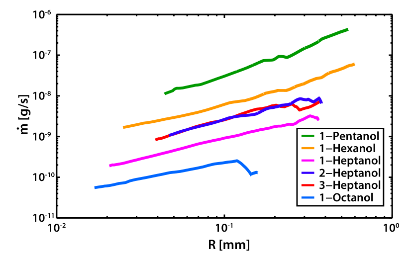
Figure 7: (color online) Rate of mass loss as a function of $R$ for droplets of different alcohols. The mass loss rates are ordered as a function of alcohol solubility, with 1-pentanol and 1-octanol being the best and least soluble alcohols, respectively.

In (convective) heat exchange problems, the heat exchange is usually expressed in terms of the (dimensionless) Nusselt-number, which is the ratio of the heat transfer rate and the rate for pure diffusion. The equivalent for solutal convection is the Sherwood number

$$\text{Sh}\equiv\frac{\left<\dot{m_{\text{d}}}\right>_{A}R}{D\Delta c}$$ (2)

where $\left<\dot{m}_{\text{d}}\right>_{A}$ is the actual (measured) mass transfer flux (rate per area), averaged over the droplet surface area $A$. This mass flux is compared to $D\Delta c/R$, the mass flux of pure (steady) diffusion from an equally sized spherical droplet (or a sessile droplet with $\theta=90^{\circ}$). In the case of pure diffusion from our sessile droplets ($45^{\circ}<\theta<75^{\circ}$), we expect to find a diffusion-limited Sherwood number $0.9<\text{Sh}_{\text{d}}<1.3$, of which the exact value depends on the droplet contact angle, as discussed in appendix B. For the case of laminar flow at high Sc-number, Bejan (1993) provides a complete and insightful derivation of the momentum equation, showing that the flow can be described using the Boussinesq approximation of the Navier-Stokes equation. This approximation assumes a slender boundary layer (i.e., $\delta_{c}\ll R$), a constant pressure over the width of the boundary layer, and a limited density difference. For high Sc numbers, the buoyant force is balanced by viscosity and it can be shown that $\delta_{c}/R\sim\text{Ra}^{-1/4}$, independent of Sc (Bejan, 1993). Here Ra is the Rayleigh number which is the ratio of the buoyant force to the damping force

$$\text{Ra}\equiv\frac{g\beta_{c}\Delta c{R}^{3}}{\nu D}$$ (3)

Taking $\delta_{c}$ as the typical length scale over which diffusion takes place in the presence of convection, we find $\left<\dot{m}_{\text{d}}\right>_{A}\sim D\Delta c/\delta_{c}$, so that

$$\text{Sh}\sim R/\delta_{c}\sim\text{Ra}^{1/4},$$ (4)

again independent of Sc. If we recast the data from figure 7 in terms of the Ra and Sh-numbers, all data sets from the six different alcohols collapse, as shown in figure 8. This figure also reveals that for large Ra, the data follow the anticipated $\text{Sh}\sim\text{Ra}^{1/4}$ scaling, which is plotted as the dashed line. For small Ra numbers, Sh converges to a plateau, as expected for diffusion. It is noteworthy that the $\text{Sh}\left(\text{Ra}\right)$ dependence from Enríquez et al. (2014), who studied the growth of CO₂ gas bubbles in slightly supersaturated water, is almost identical to our figure 8. This indicates that the flow structures around bubbles and droplets are very similar.

To better understand the transition between the convective and the diffusive behavior, and to find the value of the transition Ra-number $\text{Ra}_{\text{t}}$, we fit a crossover function of the form

$$\text{Sh}(\text{Ra})=\text{Sh}_{\text{d}}\left(1+\left(\frac{\text{Ra}}{\text{Ra}_{\text{t}}}\right)^{n}\right)^{\frac{1}{4n}}$$ (5)

to the data. Here $n$ is a fitting parameter which describes the sharpness of the transition. Equation (5) was fitted to the individual datasets of each alcohol, to obtain $\text{Ra}_{\text{t}}=12.1\pm 5.8$, $\text{Sh}_{\text{d}}=1.2\pm 0.2$, and $n=1.0\pm 0.5$. Equation (5) is plotted in figure 8, using the mean values. The fitted curve confirms that for $\text{Ra}>\text{Ra}_{\text{t}}\approx 12$, the data follows the $\text{Sh}\sim\text{Ra}^{1/4}$ scaling. A transition exists around $\text{Ra}_{\text{t}}$, where the contribution of convective mass transport gradually decreases. When $\text{Ra}<\text{Ra}_{\text{t}}$, we obtain the diffusive limit $\text{Sh}\approx 1.2$, independent of Ra.

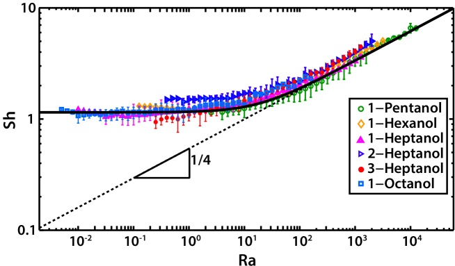
Figure 8: (color online) Sherwood number as a function of Rayleigh number. The plot shows the mean value and the spread for a total of $70$ measurements on droplets with initial volumes $2$ $\mathrm{nl}$ $\leq V_{0}\leq 1200$ $\mathrm{nl}$. Since the Ra-number depends both on the droplet size and its material properties, large $\text{Ra}-$number droplets are easily made using large droplets of 1-pentanol, whereas low Ra droplets are best studied using small droplets of the poorly soluble 1-heptanol and 1-octanol. Equation (5) is plotted as the solid black line, using $\text{Ra}_{\text{t}}=12.1$, $\text{Sh}_{\text{d}}=1.2$, and $n=1.0$.

4.2 Plume velocity

Similar to the concentration boundary layer around the droplet, the local velocity and structure of a convective plume are determined by a competition between buoyant and viscous stresses. For a thermal plume, this is described by the local thermal Rayleigh number $\text{Ra}{(z)}$, based on the local temperature difference between the center of the plume and the surroundings (see e.g. Fujii (1963) and Vázquez et al. (1996)). The local solutal Rayleigh number can be written similarly, based on the local concentration difference $\Delta c(z)$:

$$\text{Ra}(z)\equiv\frac{g\beta_{c}\Delta c(z)z^{3}}{\nu D}$$ (6)

The $\text{Ra}(z)$-number can be conveniently written in terms of $\dot{m}_{\text{d}}$ by using $\Delta c\sim\dot{m}_{\text{d}}/(Dz)$ (Fujii, 1963):

$$\text{Ra}(z)\sim\frac{g\beta_{c}\dot{m}_{\text{d}}z^{2}}{D^{2}\nu}$$ (7)

Again by exploiting the analogy with the thermal case, one finds the following scaling behaviors for the width of the plume $\delta_{c(z)}$ and the central velocity $v_{p}$ of a solutal plume with $\text{Sc}\gg 1$ (Fujii, 1963):

$$\delta_{c}\sim z\left(\text{Ra}(z)\right)^{-1/4}\propto z^{1/2}$$ (8)

$$v_{p}\sim\frac{D}{z}\left(\text{Ra}(z)\right)^{1/2}=\left(\frac{g\beta_{c}\dot{m}_{\text{d}}}{\nu}\right)^{1/2}$$ (9)

Note that $v_{p}$ is independent of $z$. We use the droplet dimension $R$ to non-dimensionalize the plume velocity, and define a plume Reynolds number:

$$\text{Re}_{p}\equiv\frac{v_{p}{R}}{\nu}$$ (10)

By using the relation for $v_{p}$ from (9) we obtain

$$\text{Re}_{p}\sim\left(\frac{g\beta_{c}\dot{m}_{\text{d}}{R}^{2}}{\nu^{3}}\right)^{1/2},$$ (11)

in which we can insert the previously found expression for $\dot{m}_{\text{d}}$ to obtain

$$\text{Re}_{p}\sim\ \text{Ra}^{5/8}\text{Sc}^{-1}$$ (12)

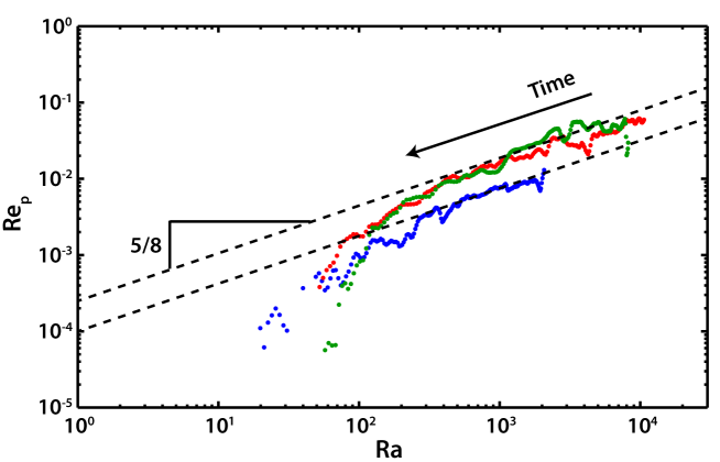
Figure 9: (color online) The plume Reynolds number as a function of Ra-number for three individual 1-pentanol droplets with $V_{0}=700$ nl (red), $V_{0}=550$ nl (green), and $V_{0}=140$ nl (blue). The expected $\text{Re}\sim\text{Ra}^{5/8}\text{Sc}^{-1}$ scaling is indeed found when $\text{Ra}\gg\text{Ra}_{\text{t}}$, but breaks down when Ra approaches $\text{Ra}_{\text{t}}$. This marks the onset of the transition region (located around $\text{Ra}_{\text{t}}$), in which convective transport is gradually exceeded by diffusive transport. To obtain the fits to the two measurements, plotted in red and blue an additional pre-factor of $0.25$ (red/green) and $0.1$ (blue) was required.

To test this scaling, we measure the maximum vertical velocity in the $\mathrm{\SIUnitSymbolMicro}$PIV data at a height of $300$ $\mathrm{\SIUnitSymbolMicro m}$ above the droplet, together with the size of the droplet and use this to calculate $\text{Re}_{p}(\text{Ra})$. The result of this analysis is shown in figure 9. For $\text{Ra}\gg\text{Ra}_{\text{t}}$, we find the anticipated $\text{Re}_{p}\sim\text{Ra}^{5/8}$. However, when Ra approaches $\text{Ra}_{\text{t}}$, a transition from convection to diffusion occurs. During and below this transition, equation (12) does not hold anymore, and the plume rapidly fades away. Note that this transition occurs when still $\text{Ra}>\text{Ra}_{\text{t}}$. For the measurements shown, there seems to be some dependence of the scaling pre-factor on the initial size of the droplet. The smallest droplet displays a somewhat lower overall plume velocity than the two larger ones. We are not yet able to pinpoint the reason for this difference. One possible hypothesis might be that inertia of the bulk flow plays a role, and that the larger droplets create a stronger convection that persists throughout the dissolution. However, more work is required to confirm or rebut this hypothesis.

5 Dissolution time

The convective flow and the related increase in mass transport was described in the previous section. In this section we proceed by deriving an expression for the convective droplet dissolution rate and associated dissolution time $\tau_{\text{c}}$. However, we start by briefly introducing diffusive dissolution, which we will use later on.

An expression for the diffusive volume loss rate $dV/dt$ has been given by Popov (2005) in the context of evaporating sessile water droplets. Popov’s solution can be rewritten to find the rate of change of the droplet, expressed in terms of the previously introduced equivalent radius $R$

$$\frac{dR}{dt}=-\frac{D\Delta c}{2\rho R}f(\theta)\left[\frac{2}{2-3\cos\theta+\cos^{3}\theta}\right]^{1/3}\sin{\theta}$$ (13)

where

$$f(\theta)=\frac{\sin(\theta)}{1+\cos(\theta)}+4\int_{0}^{\infty}\frac{1+\cosh(2\theta\epsilon)}{\sinh(2\pi\epsilon)}\tanh[(\pi-\theta)\epsilon]\mathrm{d}\epsilon$$ (14)

is a geometrical shape factor to describe the effect of the impenetrable substrate. Note that for simplicity we have neglected the intermittent contact line pinning which was observed in the experiments (Zhang et al., 2015; Dietrich et al., 2015), and equation (13) describes dissolution in the constant contact angle mode. Integration of equation (13) results in the dissolution time, with the associated diffusive timescale given by equation (1), i.e. in particular $\tau_{\text{d}}\propto R_{0}^{2}$.

We can perform a similar calculation for the convective mass exchange, again based on the cooling sphere analogy. An important difference between the cooling sphere and our dissolving droplet is that in the latter case, the radius decreases in time. However, if the dissolution is slow we can assume the process to be quasi-static and neglect this effect. We start by equating the rate of mass loss, $\dot{m}_{\text{d}}\sim-R^{2}\rho(dR/dt)>0$, to the rate at which mass is carried away in the convective plume $\dot{m}_{p}=AD\Delta c\text{Sh}/R\sim AD\Delta c\text{Ra}^{1/4}$/R, with $A\propto R^{2}$ the area of the droplet-bulk interface. From this we obtain:

$$\frac{dR}{dt}=-a\left(\frac{g\beta_{c}\Delta c_{s}^{5}D^{3}}{\nu\rho_{\text{d}}^{4}{R}}\right)^{1/4}$$ (15)

with a prefactor $a$ of order 1. Separation of variables and integrating $R$ from $R=R_{0}$ till $R=0$, and time from $t=0$ till $t=\tau_{\text{c}}$, gives the dissolution time with the associated convective time scale $\tau_{\text{c}}$ with

$$\tau_{\text{c}}=\left(\frac{\nu\rho_{\text{d}}^{4}R^{5}_{0}}{g\beta_{c}\Delta c^{5}D^{3}}\right)^{1/4}.$$ (16)

Therefore, for droplets dissolving in the convection dominated regime, we expect a dissolution time $\tau_{\text{c}}\propto{R}_{0}^{5/4}$, with a material-dependent prefactor.

To test this scaling behavior, we used the $R(t)$ curves in figures 6A and B and extracted the dissolution time from each droplet. Since the droplets could not be measured until complete dissolution, the actual value of $\tau$ had to be estimated. Therefore, we assumed that the last stage of the dissolution process was diffusion limited and extrapolated the droplet evolution by integrating equation (13), using the smallest still measured droplet size of the experiment as initial value. This extrapolation (illustrated by the green dotted line in the inset of figure 6A) provides the upper bound of $\tau$, whereas the lower bound is given by the time at which the experiment was terminated. The thus obtained values for $\tau$ are plotted as a function of $R_{0}$ for 1-pentanol and 1-heptanol in figures 6C and 6D, respectively. For larger droplets we indeed find $\tau\propto{R}_{0}^{5/4}$ as expected from equation (16), while for smaller 1-heptanol droplets $\tau\propto{R}_{0}^{2}$ is found, as expected for pure diffusion. The vertical line in figure 6D indicates $\text{Ra}=12$, showing that the transition from diffusive to convective dissolution occurs around $\text{Ra}_{\text{t}}$, consistent with our findings in section 4.

Now that we have confirmed the $\tau_{\text{c}}\propto R_{0}^{5/4}$ behavior for large droplets, we finally test whether equations (13) and (15) provide accurate descriptions of the dissolution dynamics in the diffusive and convective regimes, respectively. Moreover, we can test whether the transition between these regimes indeed occurs around $\text{Ra}_{\text{t}}=12$, as found before. To this purpose, the curves in figures 6A and 6B are replotted in figures 10A and 10B as a function of the time $t-\tau$. Figures 10C and 10D provide a close-up of the final stage of dissolution, the outlined parts of panels A and B, respectively. Along with the experimental data, we plotted the numerical integration of of the convective dissolution model, equation (15), which is the upper black line in all figures. We also plotted the diffusive dissolution model, equation (13), represented by the lower black line in each figure. All figures show that for $\text{Ra}\gg\text{Ra}_{\text{t}}$, equation (15) accurately captures the droplet dissolution process, reflecting convection-dominated dissolution. The value for the prefactor $a$ in equation (15) was adjusted for each alcohol to obtain a good fit in the convective regime. The values used are listed in table 2, along with $\theta$, for all alcohols. For $\text{Ra}\approx\text{Ra}_{\text{t}}$, the overlap between our convective model and the experiments becomes worse, consistent with the transition from convection-dominated to diffusion-dominated dissolution. The final stage of dissolution is best observed in figures 10C and 10D. When $\text{Ra}<\text{Ra}_{\text{t}}$, the dissolution is purely diffusive, reflected by the good overlap between equation (13) and the measurements. The above findings confirm the applicability of our convective dissolution model when $\text{Ra}>\text{Ra}_{\text{t}}$, and validate $\text{Ra}_{\text{t}}\approx 12$ as the transitional Ra-number for the transition from convective to diffusive dissolution dynamics.

Figure 10: (color online) Equivalent radius $R=(3V/2\pi)^{1/3}$ as a function of time to complete dissolution $t-\tau$ for 1-pentanol droplets (A) and 1-heptanol droplets (B). Panels C and D provide a zoom of the outlined parts of A and B, respectively. The upper and lower black curves in each panels represents the integration of equations (15) and (13), respectively. When $\text{Ra}>\text{Ra}_{\text{t}}=12$, equation (15) accurately describes the dissolution dynamics. Around $\text{Ra}_{\text{t}}$, which is indicated by the horizontal line in each panel, a transition exists, in which convection is progressively overtaken by diffusion. In the final stage ($\text{Ra}<\text{Ra}_{\text{t}}$), the dissolution is well described by diffusion, i.e., equation (13). The color coding for the individual measurements is the same as in figure 6.

Table 2: Value of the dimensionless prefactor $a$ in equation (15) for all alcohol types as determined from a fit to the data, together with the observed contact angles of these droplets on the PFDTS-coated substrates in water.

Alcohol	1-pentanol	1-hexanol	1-heptanol	2-heptanol	3-heptanol	1-octanol
$a$	$0.65\pm 0.05$	$0.65\pm 0.05$	$0.55\pm 0.05$	$0.65\pm 0.05$	$0.7\pm 0.05$	$0.65\pm 0.05$
$\theta$	$70^{\circ}$	$70^{\circ}$	$70^{\circ}$	$52^{\circ}$	$45^{\circ}$	$70^{\circ}$

6 Conclusion

Sessile droplets of long-chain alcohols immersed in water are ideally suited to experimentally study the basic laws of mass transfer around small objects. By choosing alcohols of different chain lengths, the alcohol’s solubility in water can be varied by almost two orders of magnitude, while its other properties remain practically the same. This large range of solubilities allowed us to vary the convective driving parameter, the Rayleigh-number, by over six orders of magnitude, while keeping the droplets large enough to visualize their shrinkage and the flow around them.

Using a combination of $\mathrm{\SIUnitSymbolMicro}$PIV and schlieren technique, we directly demonstrated that above a transition Rayleigh number $\text{Ra}_{\text{t}}\approx 12$, a buoyant flow develops around a dissolving droplet, due to the density differences between the lighter alcohol-water mixture, as compared to the heavier clean water. By modeling the observed boundary layer structure at the droplet interface and in the plume, we derived a basic scaling relation $\text{Sh}\sim\text{Ra}^{1/4}$ for convective mass transport. Using this relation as a starting point, we derived expressions for the shrinkage rate of the droplet and the velocity of the plume. In the convective regime, these models are in good agreement with our data. However, once the droplet dissolves to a size close to $\text{Ra}_{\text{t}}$, diffusion gradually overtakes convective mass transport and the convective scaling relations break down.

The observed convection and associated increase in mass transport confirms earlier work on growing bubbles in supersaturated water (Enríquez et al., 2014; Peñas López et al., 2015), indicating that it is a universal phenomenon.

The value for $\text{Ra}_{\text{t}}$ presented in this work provides an important indication to determine the dominant transport mechanism in droplet dissolution. In conjunction with this, the convective dissolution model allows for more accurate predictions of droplet dissolution times. The demonstrated predictability of the dissolution behavior of single, sessile droplets on a horizontal substrate, invites to test the derived scaling relations and fitting parameters in more complicated situations. For example, the applicability of the derived scaling relations and measured value for Ra${}_{\text{t}}$ could be tested in the context of bubble growth or droplet evaporation. Moreover, interesting changes in the flow profile can be expected, for example, when the orientation or the wettability of the substrate is changed. Other possible research directions include placing multiple droplets close together, to study their interaction, or making the droplets so large ($R>\lambda_{c}$) that they form a puddle.

Appendix A: $\mathrm{\SIUnitSymbolMicro}$PIV Data

The flow structure around the dissolving droplet has been measured using micro particle image velocimetry ($\mathrm{\SIUnitSymbolMicro}$PIV), utilizing the procedure and setup described above. In figure 11, the time evolution of the velocity field around a dissolving 1-pentanol droplet ($V_{0}=700$ nl) is shown. Shortly after deposition of the droplet (figure 1A), the data reveals the presence of a toroidal vortex above the droplet, and a strong, narrow plume originating from the droplet apex. At $600$ $\mathrm{s}$ into the dissolution process, shown in figure 11B, the center of the vortex is observed to have moved away from the droplet, causing the plume to slow down and broaden. Figure 11C shows the droplet at $2000$ $\mathrm{s}$ after deposition: the droplet has shrunk considerably, however, a small plume is still visible, along with a small mean flow, from right to left. Close to the end of the experiment ($t=2800$ $\mathrm{s}$, panel D), the droplet has almost disappeared, as has the plume. A small right-to-left mean flow is still observable.

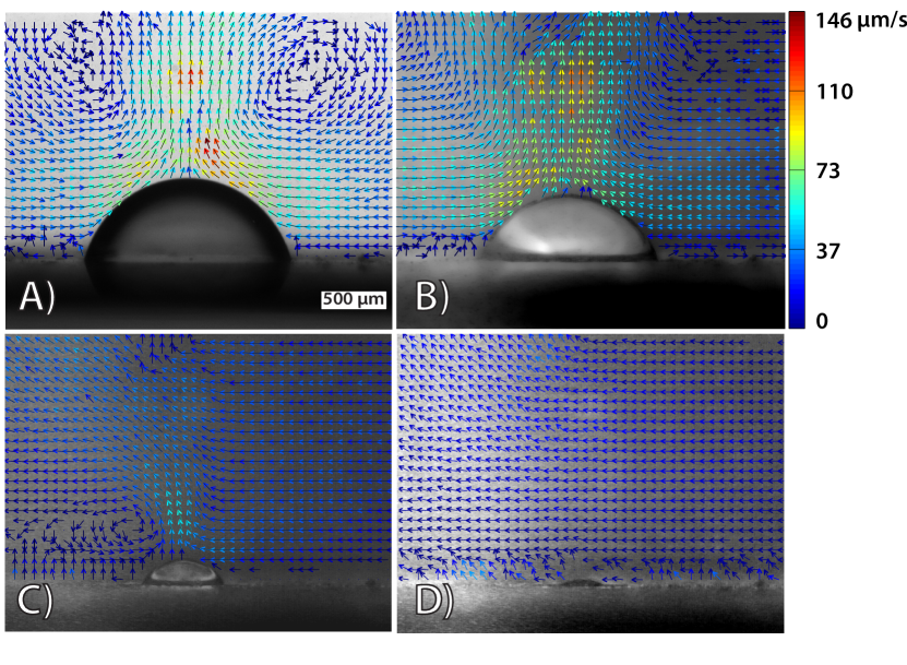
Figure 11: Velocity fields in water around a dissolving 1-pentanol droplet, 30 s after deposition of the droplet (A), and $600$ s (B), $2000$ s (C), and $2800$ s (D) after deposition.

To show that the plume is caused by solutal convection, and not simply by the presence of a spherical object at the interface, the experiment is repeated using an equally sized droplet of 1-decanol. This alcohol has negligible solubility ($c_{s}=0.037$ $\mathrm{g}\text{\,}{\mathrm{l}}^{-1}$ (Kinoshita et al., 1958)). For this droplet, $Ra\approx 10$ which means that solutal convection should be absent. The velocity field around this 1-decanol droplet is shown in figure 12. From this figure, it is clear that the presence of the droplet does not cause the formation of a plume. A slight mean flow is present, which can be seen to flow around the droplet. Although invisible from figure 2, it should be noted that in this particular experiment, tracer particles adhered to the droplet interface, something that did not happen in all other experiments where soluble droplets were studied.

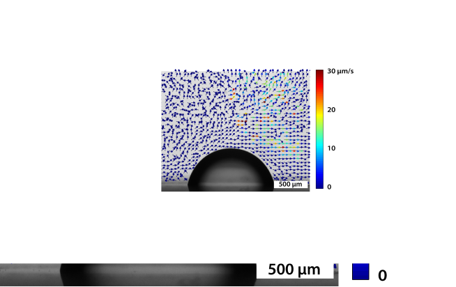
Figure 12: Velocity fields in water around an in-soluble 1-decanol droplet.

Hypothetically, the convection could be induced by surface tension gradients as well, developing over the droplet-water interface. These gradients would cause Marangoni convection over the alcohol-water interface (Kostarev et al., 2004). If this would be the case, the plume would always have the same shape and orientation with respect to the droplet and substrate, regardless the direction of gravity. To check whether this is the case, the substrate with a 1-pentanol droplet in place is mounted vertically in the center of the tank. The resulting flow, shown in figure 13, is found to be mainly parallel to the substrate. Liquid is replenished by inflow from the side and bottom, creating a large convection roll. The fact that the plume orients in a direction opposite to gravity, regardless the orientation of the substrate, confirms that the convection is buoyancy driven.

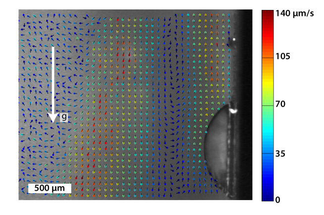
Figure 13: Velocity fields in water around a dissolving 1-pentanol droplet, sitting on a vertical wall, measured 300 s after deposition.

Appendix B: Derivation of the Sherwood number in the diffusion limited case

The Sherwood number has been defined in equation (2). In the diffusion limited case, the mass loss rate $\dot{m}$ can be calculated from the droplet properties and its size. For a spherical droplet with radius $R$, floating in an infinite bulk, the steady state mass loss is (Epstein & Plesset, 1950)

$$\frac{dm}{dt}=-4\pi RD\Delta c,$$ (17)

resulting in a Sherwood number of $\text{Sh}_{\text{d}}=1$.

For a sessile droplet, the presence of a substrate changes the dissolution, and a suitable correction factor has to be used (Popov, 2005):

$$\frac{dm}{dt}=-\pi R_{\rm{\rm{fp}}}D\Delta cf(\theta)$$ (18)

with

$$f(\theta)=\frac{\sin(\theta)}{1+\cos(\theta)}+4\int_{0}^{\infty}\frac{1+\cosh(2\theta\epsilon)}{\sinh(2\pi\epsilon)}\tanh[(\pi-\theta)\epsilon]\mathrm{d}\epsilon$$ (19)

and $R_{\rm{\rm{fp}}}$ the footprint diameter of the droplet. Using goniometry, both $R_{\rm{\rm{fp}}}$ and the droplet surface area $A$ can be expressed in terms of the volume (and thus the equivalent radius $R=(3V/2\pi)^{1/3}$), and the contact angle. From this, the Sherwood number for a sessile droplet with contact angle $\theta$, dissolving purely via diffusion is found to be

$$\text{Sh}_{\text{d}}=\frac{f(\theta)}{\sin\theta\left(1+\tan^{2}\frac{\theta}{2}\right)\left(\frac{2}{2-3\cos\theta+\cos^{3}\theta}\right)^{1/3}},$$ (20)

which indeed only depends on the droplet contact angle. Note that we defined the mass loss rate as a positive quantity, and dropped the minus sign from equation (18), resulting Sh${}_{\text{d}}>0$. By solving $f(\theta)$ numerically, $\text{Sh}_{\text{d}}(\theta)$ is plotted as the black line in figure 14. When $\theta=90$$\mathrm{\SIUnitSymbolDegree}$, the droplet has the shape of a hemisphere, and $\text{Sh}_{\text{d}}$ is equal to that of a free sphere, $\text{Sh}_{\text{d}}=1$. When $\theta>90$$\mathrm{\SIUnitSymbolDegree}$ the mass transport is reduced (as compared to that from a free sphere) and hence $\text{Sh}_{\text{d}}<1$.

When $\theta<90$$\mathrm{\SIUnitSymbolDegree}$, $\text{Sh}_{\text{d}}$ decreases towards zero, which is an implication of the choice of our characteristic length scale: For practical reasons, the equivalent radius $R$ is chosen as the characteristic length scale. In the extreme case of dissolution from a flat disk, $\theta\rightarrow 0$, $V\rightarrow 0$, and thus $R\rightarrow 0$ resulting in $\text{Sh}_{\text{d}}=0$. This does not provide a proper physical representation of the actual system, as it would result in zero mass exchange in the case of complete wetting.

Then an alternative characteristic length scale is the footprint radius $R_{\rm{\rm{fp}}}$, in which case $\text{Sh}_{\text{d}}$ is given by the red curve in figure 14. By using $R_{\rm{\rm{fp}}}$ as the characteristic length scale, $\text{Sh}_{\text{d}}$ for evaporation from a flat disk with radius $R_{\rm{fp}}$, can be calculated exactly. $f(\theta=0)=4/\pi$ (Stauber et al., 2014), which gives $\text{Sh}_{\text{d}}=\frac{4}{\pi}$. However, the drawback of using $R_{\rm{\rm{fp}}}$ as the length scale appears for $\theta>90$$\mathrm{\SIUnitSymbolDegree}$. Especially when $\theta\rightarrow 180^{\circ}$, $R_{\rm{\rm{fp}}}\rightarrow 0$, resulting once again in $\text{Sh}_{\text{d}}\rightarrow 0$.

So what experimental value for $\text{Sh}_{\text{d}}$ is expected? The Sherwood number scales mass exchange with respect to a diffusive, free, and spherical droplet. Hence $\text{Sh}_{\text{d}}=1$ when $\theta=90$$\mathrm{\SIUnitSymbolDegree}$. Due to the substrate, the mass loss from a surface droplet with $\theta<90$$\mathrm{\SIUnitSymbolDegree}$ is larger as compared to the mass exchange from the same segment of a free and spherical droplet (Hu & Larson, 2002). The opposite is true when $\theta>90^{\circ}$ (Stauber et al., 2015a). Still, $\text{Sh}_{\text{d}}$ is always of order $1$ for practical droplets ($10^{\circ}<\theta<160^{\circ}$), and independent of droplet size. The detailed dependence, as proposed in figure 14 could be the subject of future work, where small droplets (ensuring $\text{Ra}<10$) dissolve on substrates of various wettability.

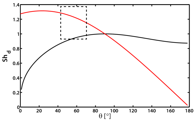
Figure 14: Diffusion limited Sherwood number $\text{Sh}_{\text{d}}$, as a function of the droplet contact angle $\theta$, calculated using the equivalent radius $R$ (black curve) or the footprint radius $R_{\text{fp}}$ (red curve), as characteristic length scale. Both curves cross at $\theta=90^{\circ}$, corresponding to a hemisphere with $R_{\text{fp}}=R$ and Sh${}_{\text{d}}=1$. The dotted region indicates the range of contact angles and experimentally observed values for $\text{Sh}_{\text{d}}$.

Acknowledegments

We gratefully acknowledge funding from The Netherlands Organisation for Scientific Research (NWO, project number 11431) and from the NWO Spinoza programme.

References

- Bejan (1993) Bejan, Adrian 1993 Heat Transfer. John Wiley & Sons, Inc.
- van der Bos et al. (2014) van der Bos, Arjan, van der Meulen, Mark-Jan, Driessen, Theo, van den Berg, Marc, Reinten, Hans, Wijshoff, Herman, Versluis, Michel & Lohse, Detlef 2014 Velocity profile inside piezoacoustic inkjet droplets in flight: Comparison between experiment and numerical simulation. Phys. Rev. Applied 1, 014004.
- Crittenden & Hixson (1954) Crittenden, Eugene D Jr. & Hixson, A. Norman 1954 Extraction of hydrogen chloride from aqueous solutions. Ind. Eng. Chem. 46, 265.
- Dehaeck et al. (2014) Dehaeck, Sam, Rednikov, Alexey & Colinet, Pierre 2014 Vapor-based interferometric measurement of local evaporation rate and interfacial temperature of evaporating droplets. Langmuir 30, 2002–2008.
- Demond & Lindner (1993) Demond, Avery H. & Lindner, Angela S. 1993 Estimation of interfacial tension between organic liquids and water. Environ. Sci. Technol. 27, 2318–2331.
- Dietrich et al. (2015) Dietrich, Erik, Kooij, E. Stefan, Zhang, Xuehua, Zandvliet, Harold J. W. & Lohse, Detlef 2015 Stick-jump mode in surface droplet dissolution. Langmuir 31, 4696–4703.
- Enríquez et al. (2014) Enríquez, Oscar R, Sun, Chao, Lohse, Detlef, Prosperetti, Andrea & van der Meer, Devaraj 2014 The quasi-static growth of bubbles. Journal of Fluid Mechanics 741, R1.
- Epstein & Plesset (1950) Epstein, P. S. & Plesset, M. S. 1950 On the stability of gas bubbles in liquid-gas solutions. J. Chem. Phys. 18, 1505–1509.
- Fujii (1963) Fujii, T. 1963 Theory of the steady laminar natural convection above a horizontal line heat source and a point heat source. Int. J. Heat Mass Transfer 6, 597–606.
- Gelderblom et al. (2011) Gelderblom, Hanneke, Marín, Álvaro G., Nair, Hrudya, van Houselt, Arie, Lefferts, Leon, Snoeijer, Jacco H. & Lohse, Detlef 2011 How water droplets evaporate on a superhydrophobic substrate. Phys. Rev. E 83, 026306.
- Hao & Leaist (1996) Hao, Ling & Leaist, Derek G. 1996 Binary mutual diffusion coefficients of aqueous alcohols. methanol to 1-heptanol. J. Chem. Eng. Data 41, 210–213.
- Høiland & Vikingstad (1976) Høiland, Harald & Vikingstad, Einar 1976 Partial molal volumes and additivity of group partial molal volumes of alcohols in aqueous solution at 25∘c and 35∘c. Acta Chemica Scandinavica A 30, 182–186.
- Hu & Larson (2002) Hu, Hua & Larson, Ronald G. 2002 Evaporation of a sessile droplet on a substrate. J. Phys. Chem. B. 106, 1334–1344.
- Karpitschka (2012) Karpitschka, S. 2012 Dynamics of liquid interfaces with compositional gradients. PhD thesis, Universität Potsdam.
- Kelly-Zion et al. (2013a) Kelly-Zion, P.L., Pursell, Christopher J., Hasbamrer, N, Cardozo, B, Gaughan, K & Nickels, Kevin 2013a Vapor distribution above an evaporating sessile drop. International Journal of Heat and Mass Transfer 65, 165–172.
- Kelly-Zion et al. (2013b) Kelly-Zion, P. L., Batra, J. & Pursell, C.J. 2013b Correlation for the convective and diffusive evaporation of a sessile drop. International Journal of Heat and Mass Transfer 64, 278 – 285.
- Kinoshita et al. (1958) Kinoshita, Kyoji, Ishikawa, Hidehiko & Shinoda, Kōzō 1958 Solubility of alcohols in water determined the surface tension measurements. Bulletin of the Chemical Society of Japan 31, 1081–1082.
- Kostarev et al. (2004) Kostarev, K, Zuev, Andrew & Viviani, Antonio 2004 Oscillatory marangoni convection around the air bubble in a vertical surfactant stratification. Comptes Rendus Mécanique 332, 1 – 7.
- Lohse & Zhang (2015) Lohse, Detlef & Zhang, Xuehua 2015 Surface nanobubbles and nanodroplets. Rev. Mod. Phys. 87, 981–1035.
- Peñas López et al. (2015) Peñas López, Pablo, Parrales, Miguel A. & Rodríguez-Rodríguez, Javier 2015 Dissolution of a spherical cap bubble adhered to a flat surface in air-saturated water. Journal of Fluid Mechanics 775, 53–76.
- Picknett & Bexon (1977) Picknett, R.G. & Bexon, R 1977 The evaporation of sessile or pendant drops in still air. Journal of Colloid and Interface Science 61, 336 – 350.
- Popov (2005) Popov, Yuri O. 2005 Evaporative deposition patterns: Spatial dimensions of the deposit. Phys. Rev. E 71, 036313.
- Raffel et al. (2007) Raffel, Markus, Willert, Christian E, Wereley, Steve T & Kompenhans, Jürgen 2007 Particle Image Velocimetry. Springer.
- Romero et al. (2007) Romero, Carmen M., Suárez, Andrés F. & Jiménez, Eulogio 2007 Effect of temperature on the volumetric properties of aliphatic alcohols in dilute aqueous solutions. Rev. Colomb. Quím. 36, 377–386.
- Settles (2001) Settles, G.S. 2001 Schlieren and Shadowgraph Techniques. Springer-Verlag.
- Shahidzadeh-Bonn et al. (2006) Shahidzadeh-Bonn, Noushine, Rafaï, Salima, Azouni, Aza & Bonn, Daniel 2006 Evaporating droplets. Journal of Fluid Mechanics 549, 307–313.
- Somasundaram et al. (2015) Somasundaram, S., Anand, T. N. C. & Bakshi, Shamit 2015 Evaporation-induced flow around a pendant droplet and its influence on evaporation. Physics of Fluids 27, 112105.
- Stauber et al. (2014) Stauber, J.M., Wilson, S.K., Duffy, B.R. & Sefiane, K. 2014 On the lifetimes of evaporating droplets. J. Fluid Mech. 744, R2.
- Stauber et al. (2015a) Stauber, Jutta M., Wilson, Stephen K. & Duffy, Brian R. 2015a Evaporation of droplets on strongly hydrophobic substrates. Langmuir 31, 3653–3660.
- Stauber et al. (2015b) Stauber, Jutta M., Wilson, Stephen K., Duffy, Brian R. & Sefiane, Khellil 2015b On the lifetimes of evaporating droplets with related initial and receding contact angles. Physics of Fluids 27, 122101.
- Stephenson et al. (1984) Stephenson, Richard, Stuart, James & Tabak, Mary 1984 Mutual solubility of water and aliphatic alcohols. Journal of Chemical & Engineering Data 29, 287–290.
- Vázquez et al. (1996) Vázquez, P. A., Pérez, A. T. & Castellanos, A. 1996 Thermal and electrohydrodynamic plumes. a comparative study. Physics of Fluids 8, 2091–2096.
- Yalkowsky et al. (2010) Yalkowsky, S.H., He, Y. & Jain, P. 2010 Handbook of Aqueous Solubility Data, Second Edition. Taylor & Francis.
- Zhang et al. (2015) Zhang, Xuehua, Wang, Jun, Bao, Lei, Dietrich, Erik, van der Veen, Roeland C. A., Peng, Shuhua, Friend, James, Zandvliet, Harold J. W., Yeo, Leslie & Lohse, Detlef 2015 Mixed mode of dissolving immersed nanodroplets at a solid-water interface. Soft Matter 11, 1889–1900.