Magnetic helicity in non-axisymmetric mean-field solar dynamo.

Abstract

The paper address the effects of magnetic helicity conservation in a non-linear non-axisymmetric mean-field solar dynamo model. We study the evolution of the shallow non-axisymmetric magnetic field perturbation with the strength about 10G in the solar convection zone. The dynamo evolves from the pure axisymmetric stage through the short (about 2 years) transient phase when the non-axisymmetric m=1 dynamo mode is dominant to the final stage where the axisymmetry of the dynamo is almost restored. It is found that magnetic helicity is transferred forth and back over the spectral space during the transient phase. Also our simulations shows that the non-axisymmetric distributions of magnetic helicity tend to follows the regions of the Hale polarity rule.

1 Introduction

Conservation of the magnetic helicity is significant for many physical process above and beneath the solar photosphere. After seminal papers [1] and [2] it was understood that the magnetic helicity is one of the key parameters which determine generation and evolution of the large-scale magnetic field in the solar dynamo. It is commonly believed that the solar magnetic fields are generated by the axisymmetric hydromagnetic dynamo instability in the solar convection zone due to the differential rotation and helical convective motions. Effects of magnetic helicity conservation in the axisymmetric dynamo inside convection zone and their impact on the activity in the regions above the photosphere are lively debated in the current literature (see, e.g., [3]). Despite the strong axisymmetry of solar magnetic activity on the long time-scale, deviations from the axisymmetry are rather strong at any particular moment of observations.

For the physical conditions of the modern Sun it was found that the large-scale non-axisymmetric magnetic field is linearly stable [4]. Using the nonlinear mean-field model, in [5] was found that the non-axisymmetric magnetic perturbations can result to transients in evolution of the axisymmetric fields if the perturbations are anchored to level of the rotational subsurface shear layer ($\approx 0.9R$). After relaxation of the non-axisymmetric magnetic perturbation the non-linear dynamo processes can maintain a weak non-axisymmetric field in expense of the axisymmetric magnetic field. It was also found that that the magnetic helicity conservation affects the interaction of the non-axisymmetric and axisymmetric magnetic fields.

The goal of the paper is to study the evolution of the magnetic helicity density using the non-axisymmetric mean-field dynamo model. Also, we are interesting to study redistribution of magnetic helicity density over the partial azimuthal modes (see [6]) of the large-scale magnetic field. The model was described in details in [5]. In the next two sections we briefly outline the basic equations of our model and discuss mechanisms of the non-linear interactions between the axisymmetric andd non-axisymmetric dynamos. The Section 4 contain the description of main results, discussion and the Section 5 summarizes conclusions of the study.

2 Basic equations

Evolution of the large-scale magnetic field in perfectly conductive media is described by the mean-field induction equation [6]:

$$\partial_{t}\left\langle\mathbf{B}\right\rangle=\boldsymbol{\nabla}\times\left(\mathbf{\boldsymbol{\boldsymbol{\mathcal{E}}}+}\left\langle\mathbf{U}\right\rangle\times\left\langle\mathbf{B}\right\rangle\right)$$ (1)

where $\boldsymbol{\mathcal{E}}=\left\langle\mathbf{u\times b}\right\rangle$ is the mean electromotive force; $\mathbf{u}$ and $\mathbf{b}$ are the turbulent fluctuating velocity and magnetic field respectively; and $\left\langle\mathbf{U}\right\rangle$ and $\left\langle\mathbf{B}\right\rangle$ are the mean velocity and magnetic field. For convenience we decompose the magnetic field into the axisymmetric, (hereafter $\overline{\mathbf{B}}$-field), and non-axisymmetric parts, (hereafter $\tilde{\mathbf{B}}$-field): $\left\langle\mathbf{B}\right\rangle=\overline{\mathbf{B}}+\tilde{\mathbf{B}}$. We assume that the mean flow is axisymmetric $\left\langle\mathbf{U}\right\rangle\equiv\overline{\mathbf{U}}$. Let $\hat{\boldsymbol{\phi}}=\mathbf{e_{\phi}}$ and $\hat{\mathbf{r}}=r\mathbf{e}_{r}$ be vectors in the azimuthal and radial directions respectively, then we represent the mean magnetic field vectors as follows:

$$\left\langle\mathbf{B}\right\rangle = \overline{\mathbf{B}}+\tilde{\mathbf{B}}$$ (2)

$$\mathbf{\overline{B}} = \hat{\boldsymbol{\phi}}B+\nabla\times\left(A\hat{\boldsymbol{\phi}}\right)$$ (3)

$$\tilde{\mathbf{B}} = \boldsymbol{\nabla}\times\left(\hat{\mathbf{r}}T\right)+\boldsymbol{\nabla}\times\boldsymbol{\nabla}\times\left(\hat{\mathbf{r}}S\right),$$ (4)

where $A$, $B$, $T$ and $S$ are scalar functions representing the axisymmetric and non-axisymmetric parts respectively. Assuming that $A$ and $B$ do not depend on longitude, Eqs(3, 4) ensure that the field $\left\langle\mathbf{B}\right\rangle$ is divergence-free. The integration domain includes the solar convection zone from $0.71$ to $0.99R_{\odot}$. The distribution of the mean flows is given by helioseismology ([7]). Profiles of the angular velocity is the same as in [5], (see Figure 1 there). For the sake of simplicity we neglect the meridional circulation in the model.

We use formulation for the mean electromotive force obtained in form:

$$\mathcal{E}_{i}=\left(\alpha_{ij}+\gamma_{ij}\right)\left\langle B\right\rangle_{j}-\eta_{ijk}\nabla_{j}\left\langle B\right\rangle_{k}.$$ (5)

where symmetric tensor $\alpha_{ij}$ models the generation of magnetic field by the $\alpha$- effect; antisymmetric tensor $\gamma_{ij}$ controls the mean drift of the large-scale magnetic fields in turbulent medium; tensor $\eta_{ijk}$ governs the turbulent diffusion. We take into account the effect of rotation and magnetic field on the mean-electromotive force (see, e.g., [8] for details). To determine unique solution we apply the following gauge (see, e.g., [6]):

$$\int_{0}^{2\pi}\int_{-1}^{1}Sd\mu d\phi=0,\,\,\int_{0}^{2\pi}\int_{-1}^{1}Td\mu d\phi=0,$$ (6)

where $\mu=\cos\theta$ and $\theta$ is the polar angle..

3 Nonlinear interaction of the axisymmetric and non-axisymmetric modes

Interaction between the axisymmetric and non-axisymmetric modes in the mean-field dynamo models can be due to nonlinear dynamo effects, for example, the $\alpha$-effect, [9, 10]. In our model the $\alpha$ effect takes into account the kinetic and magnetic helicities in the following form:

$$\alpha_{ij} = C_{\alpha}\sin^{2}\theta\psi_{\alpha}(\beta)\alpha_{ij}^{(H)}\eta_{T}+\alpha_{ij}^{(M)}\frac{\left\langle\chi\right\rangle\tau_{c}}{4\pi\overline{\rho}\ell^{2}}$$ (7)

where $C_{\alpha}$ is a free parameter which controls the strength of the $\alpha$- effect due to turbulent kinetic helicity; $\alpha_{ij}^{(H)}$ and $\alpha_{ij}^{(M)}$ express the kinetic and magnetic helicity parts of the $\alpha$-effect, respectively; $\eta_{T}$ is the magnetic diffusion coefficient, and $\left\langle\chi\right\rangle=\left\langle\mathbf{a}\cdot\mathbf{b}\right\rangle$ the helicity density of the small-scale magnetic field ( $\mathbf{a}$ and $\mathbf{b}$ are the fluctuating parts of magnetic field vector-potential and magnetic field vector). Both the $\alpha_{ij}^{(H)}$ and $\alpha_{ij}^{(M)}$ depend on the Coriolis number $\Omega^{*}=4\pi{\displaystyle\frac{\tau_{c}}{P_{rot}}}$, where $P_{rot}$ is the rotational period, $\tau_{c}$ is the convective turnover time, and $\ell$ is a typical length of the convective flows (the mixing length). Function $\psi_{\alpha}(\beta)$ controls the so-called “algebraic” quenching of the $\alpha$- effect where $\beta=\left|\mathbf{\left\langle B\right\rangle}\right|/\sqrt{4\pi\overline{\rho}u^{\prime 2}}$, $u^{\prime}$ is the r.m.s. of the convective velocity.

The magnetic helicity conservation results to the dynamical quenching of the dynamo. Contribution of the magnetic helicity to the $\alpha$-effect is expressed by the second term in Eq.(7). The magnetic helicity density of turbulent field, $\left\langle\chi\right\rangle$, is governed by the conservation law [11]:

$$\frac{\partial\left\langle\chi\right\rangle^{(tot)}}{\partial t}=-\frac{\left\langle\chi\right\rangle}{R_{m}\tau_{c}}-2\eta\left\langle\mathbf{B}\right\rangle\cdot\left\langle\mathbf{J}\right\rangle-\boldsymbol{\nabla\cdot}\boldsymbol{\boldsymbol{\mathcal{F}}}^{\chi},$$ (8)

where $\left\langle\chi\right\rangle^{(tot)}=\left\langle\chi\right\rangle+\left\langle\mathbf{A}\right\rangle\cdot\left\langle\mathbf{B}\right\rangle$ is the total magnetic helicity density of the mean and turbulent fields, $\boldsymbol{\boldsymbol{\mathcal{F}}}^{\chi}=-\eta_{\chi}\boldsymbol{\nabla}\left\langle\chi\right\rangle$ is the diffusive flux of the turbulent magnetic helicity, and $R_{m}$ is the magnetic Reynolds number. The coefficient of the turbulent helicity diffusivity, $\eta_{\chi}$, is chosen ten times smaller than the isotropic part of the magnetic diffusivity [12]: $\eta_{\chi}=\frac{1}{10}\eta_{T}$. Similarly to the magnetic field, the mean magnetic helicity density can be formally decomposed into the axisymmetric and non-axisymmetric parts: $\left\langle\chi\right\rangle^{(tot)}=\overline{\chi}^{(tot)}+\tilde{\chi}^{(tot)}$. The same can be done for the magnetic helicity density of the turbulent field: $\left\langle\chi\right\rangle=\overline{\chi}+\tilde{\chi}$, where $\overline{\chi}=\overline{\mathbf{a}\cdot\mathbf{b}}$ and $\tilde{\chi}=\tilde{\left\langle\mathbf{a}\cdot\mathbf{b}\right\rangle}$. Then we have,

$$\overline{\chi}^{(tot)} =\overline{\chi}+\overline{\mathbf{A}}\cdot\overline{\mathbf{B}}+\overline{\tilde{\mathbf{A}}\cdot\tilde{\mathbf{B}}},$$ (9)

$$\tilde{\chi}^{(tot)} =\tilde{\chi}+\overline{\mathbf{A}}\cdot\tilde{\mathbf{B}}+\tilde{\mathbf{A}}\cdot\overline{\mathbf{B}}+\tilde{\mathbf{A}}\cdot\tilde{\mathbf{B}},$$ (10)

Evolution of the $\overline{\chi}$ and $\tilde{\chi}$ is governed by the corresponding parts of Eq(8). Thus, the model takes into account contributions of the axisymmetric and non-axisymmetric fields in the whole magnetic helicity density balance, providing a non-linear coupling. We see that the $\alpha$-effect is dynamically linked to the longitudinally averaged magnetic helicity of the non-axisymmetric $\tilde{\mathbf{B}}$-field, which is the last term in Eq(9). Thus, the nonlinear $\alpha$-effect is non-axisymmetric, and it results in coupling between the axisymmetric and non-axisymmetric modes. The coupling works in both directions. For instance, the azimuthal $\alpha$-effect results in $\mathcal{E}_{\phi}=\alpha_{\phi\phi}\left\langle B_{\phi}\right\rangle$. If we denote the non-axisymmetric part of the $\alpha_{\phi\phi}$ by $\tilde{\alpha}_{\phi\phi}$ then the mean electromotive force is $\overline{\mathcal{E}}_{\phi}=\overline{\alpha}_{\phi\phi}\overline{B}_{\phi}+\overline{\tilde{\alpha}_{\phi\phi}\tilde{B}_{\phi}}$. This introduces a new generation source which is usually ignored in the axisymmetric dynamo models.

The numerical scheme employs the spherical harmonics decomposition for the non-axisymmetric part of the problem and the finite differences in radial direction. The axisymmetric part of the problem was integrated using the pseudo-spectral method in latitudinal direction and the finite differences in radial direction. The parameters of the solar convection zone are taken from Stix[13] and they were described in [5]. At the bottom of the convection zone we set up a perfectly conducting boundary condition for the axisymmetric magnetic field, and for the non-axisymmetric field we set the functions $S$ and $T$ to zero. At the top of the convection zone the poloidal field is smoothly matched to the external potential field. The magnetic helicity conservation is determined by the magnetic Reynolds number $R_{m}$. In this paper we employ $R_{m}=10^{4}$.

The axisymmetric field was started from a developed non-linear stage. This stage is characterized by the established oscillating dynamo waves drifting from the bottom to the top of the convection zone. In subsurface shear layer the wave of the axisymmetric toroidal magnetic field is deflected equator-ward. The model satisfactory reproduce the sunspot activity time-latitude diagram and reversals of the polar magnetic fields as results of dynamo wave of the axisymmetric poloidal magnetic fields.

Previously, it was found that in the nonlinear non-axisymmetric solar dynamo the non-axisymmetric magnetic field relax to the stage where its energy is about factor $10^{-6}$ off the equipartition level of the energy of the convective motions. However, the strong non-axisymmetric magnetic field could be maintained by the periodic seed from a decaying active regions or other process. In the paper we do not concern this important issue. Instead we restrict our study by the case of the single perturbation. For the seed field we consider a non-symmetric relative to the equator perturbation represented by a sum of the equatorial dipole (l=1, m=$\pm$1,2) and quadrupole ($l=2$, $m=\pm 1,2$) components (see [5]). We employ the initial non-axisymmetric perturbation to be concentrated in the near-surface shear layer.

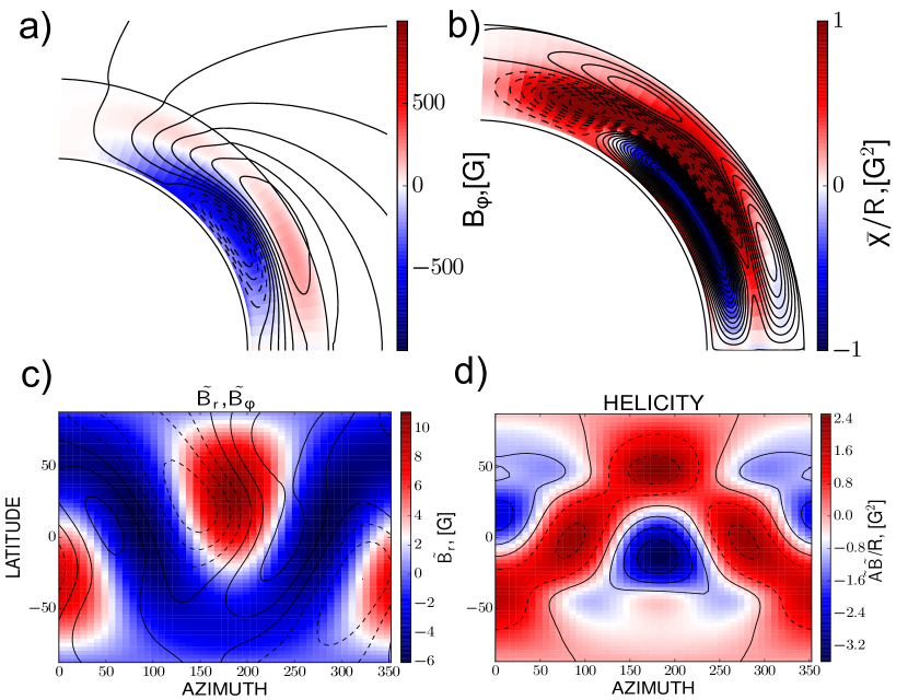
Figure 1: . Distribution of the axisymmetric and non-axisymmetric magnetic field just after initialization : a) the axisymmetric magnetic field in meridional cross-section, the geometry of the poloidal field is shown by contours; b) Color image shows the magnetic helicity density $\bar{\chi}$ and the $\overline{\mathbf{A}}\cdot\overline{\mathbf{B}}$ is shown by contours. It varies in the same range as the $\bar{\chi}$ ; c) color image shows the non-axisymmetric $\tilde{B_{r}}$ at the surface and contours show the azimuthal component of the non-axisymmetric magnetic field, $\tilde{B}_{\phi}$; d) color image shows distribution of the $\tilde{\mathbf{A}}\cdot\tilde{\mathbf{B}}$ and contours are for the non-axisymmetric part of the small-scale magnetic helicity density, $\tilde{\chi}$, which varies in the same interval of magnitude as the $\tilde{\mathbf{A}}\cdot\tilde{\mathbf{B}}$ .

4 Results and discussion

Distribution of the axisymmetric and non-axisymmetric magnetic field just after initialization is shown by Figure1(a,c). The dynamic of the system is started to evolve at the epoch of the solar minimum when the polar field has maximum amplitude and the strength of the toroidal field in the near-surface layer is minimal. Figure 1(b,c) show distributions of the magnetic helicity density for the axisymmetric and the non-axisymmetric parts respectively. At the Northern hemisphere the axisymmetric part of the small-scale magnetic helicity is negative near the bottom of the convection where the dynamo wave of the axisymmetric toroidal magnetic field zone is concentrated. Also we have the negative patch of the $\bar{\chi}$ at the near surface where the dynamo wave from the previous cycle is decaying. Note that the $\overline{\mathbf{A}}\cdot\overline{\mathbf{B}}$ is positive at the North and the sign of it is in balance with the sign of the $\bar{\chi}$ because of the helicity conservation in the model. At the initialization time the non-axisymmetric perturbation is of the strength about 10G at the surface and it decays to zero at the $r=0.9R$. Form Figure 1 it is seen that the injected helicity density of the non-axisymmetric magnetic field is about factor 2 larger than the helicity density of the axisymmetric part of the magnetic field..

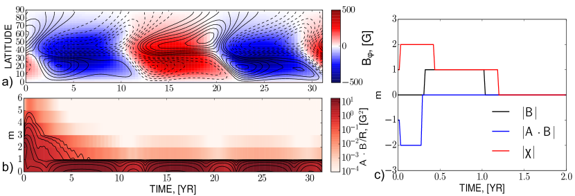
Figure 2: . a) Time-latitude diagram of the axisymmetric toroidal magnetic field at the r=0.9R (color image), contours show the radial magnetic field at the surface (they vary in range $\pm 5$G); b) Color image show variations of the integral of the $\left|\mathbf{\left\langle A\right\rangle\cdot}\left\langle\mathbf{B}\right\rangle\right|$ over latitudes with time at the r=0.9R. The first six partial dynamo modes are shown (m=0 corresponds to the axisymmetric magnetic field). Contours show the same for the small-scale helicity density, which varies within the same range of magnitudes as the $\left|\mathbf{\left\langle A\right\rangle\cdot}\left\langle\mathbf{B}\right\rangle\right|$; c) The number of the partial non-axisymmetric mode which has the strongest magnitude of the magnetic field (black line), the helicity density of the large-scale magnetic field (blue line, the number was reverted to avoid the overlap), and the small-scale magnetic helicity density (red line).

Figure 2(a) shows the time-latitude evolution of the axisymmetric magnetic field near the solar surface. Note that in compare with results of the previous paper, [5], the butterfly diagram is unchanged after initialization of the non-axisymmetric perturbation because the initialization time in these simulations corresponds to epoch of the minimum of the dynamo cycle. Figure 2(b) shows variations of the $\int\left|\left\langle\mathbf{A}\right\rangle\cdot\left\langle\mathbf{B}\right\rangle\right|d\mu$ at the radial distance $r=0.95R$. The first six partial dynamo modes are shown (m=0 corresponds to the axisymmetric magnetic field). It is seen that after initialization the helicity is transferred from the non-axisymmetric modes to the axisymmetric magnetic field. Figure 2(c) gives a more detailed information about redistribution of the magnetic energy and magnetic helicity among the partial modes of the non-axisymmetric magnetic field in the dynamo for period of the first two years after initialization. It is seen that for the short period about half an year after initialization the non-axisymmetric m=1 dynamo mode become the dominant. This happens after the maximum of the helicity density transfer to the m=2 modes.

The strength of the non-axisymmetric magnetic field decays at the time about 5 year to the level which is about $10^{-3}$off the strength of the axisymmetric magnetic field. The nonlinear interaction of the axisymmetric and non-axisymmetric magnetic fields via magnetic helicity helps to maintain the non-axisymmetric magnetic field from a complete decay.

Figure 3,4 show the snapshot of magnetic helicity density and the large-scale magnetic field distributions at the surface and configurations of the magnetic field above the photosphere during the transient phase (at the time of one year after initialization) and three years after. The initialization epoch corresponds to the minimum of the dynamo cycle. Due to this fact the dynamo model demonstrate inversions of the hemispheric helicity rule. This is supported from observations [14, 15] and axisymmetric dynamo models [11, 16]. It is interesting that the non-axisymmetric helicity density distribution tends to follow to patterns of the large-scale non-axisymmetric magnetic field during evolution. Therefore, according to our model the change of the helicity sign in the longitudinal direction could occurs at the sectoral boundaries of the large-scale magnetic field. During the transient phase of evolution the axisymmetric toroidal field at the near surface layer is positive in the Northern hemisphere and it is negative in the Southern hemisphere. The Figure 3(b) shows that in the Northern hemisphere the helicity density changes the sign from negative to positive at the anti-Hale sectoral boundary ([17]) and in opposite direction at the sectoral boundary which correspond to the Hale polarity rule for the given cycle. This is probably because of the local balance of the magnetic helicity for the large and small scales which is prescribed by simple anzatz given by Eq.(8). It is interesting to note that the flare activity is concentrated near the anti-Hale sectorial boundaries [17].

Figure 4 shows that about three years after initialization the model restores the dominance of the axisymmetric magnetic fields. The hemispheric helicity sign rule is also restored to the normal case when the Northern hemisphere has the negative sign of the magnetic helicity and the Southern has positive one.

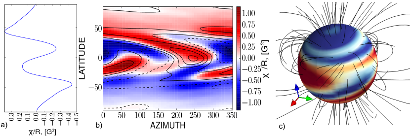
Figure 3: Snapshots of the magnetic helicity density and magnetic field distributions at the time one year after initialization of the non-axisymmetric perturbation: a) mean small-scale helicity density, $\bar{\chi}$; b) color image shows the sum of the non-axisymmetric and axisymmetric parts of the magnetic helicity density, $\left\langle\chi\right\rangle=\overline{\chi}+\tilde{\chi}$, contours show the strength of the radial magnetic field (within the range of $\pm 10$G);c) shows magnetic field lines and color image shows the strength of the radial magnetic field.

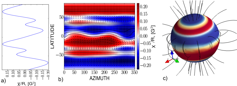
Figure 4: The same as Figure 3 for the time three years after initialization of the non-axisymmetric perturbation.

5 Conclusions

The main goal of the paper was to illustrate some effects of the magnetic helicity conservation in the non-axisymmetric dynamo model. It was found that the non-axisymmetric perturbations goes through the transient phase when the maximum of the magnetic energy in the near surface layer shift from the m=0 dynamo mode (the axisymmetric magnetic field) to the m=1 mode. At the same time the magnetic helicity density is transferred over the spectral modes in the same direction at the beginning of the transient phase and back shortly after while. Our simulations shows that the non-axisymmetric distributions of the small-scale magnetic helicity tend to follows the regions of the Hale polarity rule. The study is restricted to the case of the single perturbation at the particular moment of the dynamo cycle. Thus it would be interesting to extend our investigation for a more general case including a more realistic form of the non-axisymmetric perturbations.

Acknowledgments The work supported by RFBR under grants 14-02-90424, 15-02-01407 and the project II.16.3.1 of ISTP SB RAS.

References

- [1] U. Frisch, A. Pouquet, J. Léorat, and M. A. Possibility of an inverse cascade of magnetic helicity in magnetohydrodynamic turbulence. J. Fluid Mech., vol. 68 (1975), pp. 769–778.
- [2] A. Pouquet, U. Frisch, and J. Léorat. Strong MHD helical turbulence and the nonlinear dynamo effect. J. Fluid Mech., vol. 68 (1975), pp. 769–778.
- [3] A. Brandenburg and K. Subramanian. Astrophysical magnetic fields and nonlinear dynamo theory. Phys. Rep., vol. 417 (2005), pp. 1–209.
- [4] K.-H. Raedler. Investigations of spherical kinematic mean-field dynamo models. Astronomische Nachrichten, vol. 307 (1986), pp. 89–113.
- [5] V. V. Pipin and A. G. Kosovichev. Effects of large-scale non-axisymmetric perturbations in the mean-field solar dynamo. ApJ, 813, 134, (2015).
- [6] F. Krause and K.-H. Rädler. Mean-Field Magnetohydrodynamics and Dynamo Theory (Berlin: Akademie-Verlag, 1980).
- [7] R. Howe, T. P. Larson, J.Schou, F.Hill, R. Komm, J. Christensen-Dalsgaard, & M. J. Thompson First Global Rotation Inversions of HMI Data. Journal of Physics Conference Series, vol. 271 (2011), no. 1, p. 012061.
- [8] V. V. Pipin. Dependence of magnetic cycle parameters on period of rotation in non-linear solar-type dynamos. MNRAS, vol. 451 (2015), pp. 1528–1539.
- [9] K.-H. Rädler, E. Wiedemann, A. Brandenburg, R. Meinel, & I. Tuominen Nonlinear mean-field dynamo models - Stability and evolution of three-dimensional magnetic field configurations. A&A, vol. 239 (1990), pp. 413–423.
- [10] D. Moss. Non-axisymmetric solar magnetic fields. MNRAS, vol. 306 (1999), pp. 300–306.
- [11] V. V. Pipin, H. Zhang, D. D. Sokoloff, K. M. Kuzanyan, & Y. Gao The origin of the helicity hemispheric sign rule reversals in the mean-field solar-type dynamo. MNRAS, vol. 435 (2013), pp. 2581–2588.
- [12] D. Mitra, S. Candelaresi, P. Chatterjee, R. Tavakol, & A. Brandenburg Equatorial magnetic helicity flux in simulations with different gauges. Astronomische Nachrichten, vol. 331 (2010), pp. 130–+.
- [13] M. Stix. The sun: an introduction (Berlin : Springer, 2002), 2 ed.
- [14] H. Zhang, T. Sakurai, A. Pevtsov, Y. Gao, H. Xu, D. D. Sokoloff, & K. Kuzanyan A new dynamo pattern revealed by solar helical magnetic fields. MNRAS, vol. 402 (2010), pp. L30–L33.
- [15] S. Gosain, A. A. Pevtsov, G. V. Rudenko, and S. A. Anfinogentov. First Synoptic Maps of Photospheric Vector Magnetic Field from SOLIS/VSM: Non-radial Magnetic Fields and Hemispheric Pattern of Helicity. ApJ, vol. 772 (2013), p. 52.
- [16] D. Sokoloff, H. Zhang, D. Moss, N. Kleeorin, K. Kuzanyan, I. Rogachevski, Y. Gao, H. Xu Current helicity constraints in solar dynamo models. In A. G. Kosovichev, E. de Gouveia Dal Pino, and Y. Yan, editors, IAU Symposium (2013), vol. 294 of IAU Symposium, pp. 313–318.
- [17] L. Svalgaard, I. G. Hannah, and H. S. Hudson. Flaring Solar Hale Sector Boundaries. ApJ, vol. 733 (2011), p. 49.