A Theory of Local Matching
SIFT and Beyond

Abstract

Why has SIFT been so successful? Why its extension, DSP-SIFT, can further improve SIFT? Is there a theory that can explain both? How can such theory benefit real applications? Can it suggest new algorithms with reduced computational complexity or new descriptors with better accuracy for matching? We construct a general theory of local descriptors for visual matching. Our theory relies on concepts in energy minimization and heat diffusion. We show that SIFT and DSP-SIFT approximate the solution the theory suggests. In particular, DSP-SIFT gives a better approximation to the theoretical solution; justifying why DSP-SIFT outperforms SIFT. Using the developed theory, we derive new descriptors that have fewer parameters and are potentially better in handling affine deformations.

1 Introduction

Questions:

Why has SIFT been so successful? Why DSP-SIFT [Dong and Soatto, 2015] can further improve SIFT? Is there a theory that can explain both? How can such theory benefit real applications? Can it suggest new algorithms with reduced computational complexity or new descriptors with better accuracy for matching?

Contributions:

We construct a general theory of local descriptors for visual matching. Our theory relies on concepts in energy minimization and heat diffusion. We show that SIFT and DSP-SIFT approximate the solution the theory suggests. In particular, DSP-SIFT gives a better approximation to the theoretical solution; justifying why DSP-SIFT outperforms SIFT. We derive new algorithms based on this theory. Specifically, we present a computationally efficient approximation to DSP-SIFT algorithm [Dong and Soatto, 2015] by replacing the sampling procedure in DSP-SIFT with a closed-form approximation that does not need any sampling. This leads to a significantly faster algorithm compared to DSP-SIFT. In addition, we derive new descriptors directly from this theory. The new descriptors have fewer parameters as well as the potential of better handling affine deformations, compared to SIFT and DSP-SIFT.

2 Contributions

Throughout this text, isotropic multivariate Gaussian kernel and periodic univariate Gaussian are denoted by $k$ and $\tilde{k}$,

$$k_{\sigma}(\boldsymbol{x})\triangleq(2\pi\sigma^{2})^{-\dim(\boldsymbol{x})}\,e^{-\frac{\|\boldsymbol{x}\|^{2}}{2\sigma^{2}}}\quad,\quad\tilde{k}_{\sigma}(\phi)\triangleq\sum_{k=-\infty}^{\infty}k_{\sigma}(\phi+2\pi k)\,.$$ (1)

Consider an image $f$. Given an origin-centered detected key point $\boldsymbol{x}$ with assigned scale $\sigma$ and orientation $\beta$. The continuous form of a SIFT descriptor can be expressed as [Dong et al., 2015, Vedaldi and Fulkerson, 2010],

$$h_{SIFT}(\beta,\boldsymbol{x})\triangleq\int_{\mathcal{X}}\tilde{k}_{\sigma_{r}}(\beta-\angle\nabla f(\boldsymbol{y}))\,k_{\sigma_{d}}(\boldsymbol{y}-\boldsymbol{x})\,\|\nabla f(\boldsymbol{y})\|\,d\boldsymbol{y}\,,$$ (2)

where $\sigma_{r}$ resembles the size of each orientation bin, e.g. $\frac{2\pi}{8}$ for $8$ bins. $\sigma_{d}$ determines the spatial support of the descriptor as a function of $\sigma$, e.g. $\sigma_{d}\triangleq 3\sigma$.

By observing that the above descriptor is pooling (weighted averaging) across displacement, [Dong et al., 2015] adds domain size pooling to this construction and suggests,

$$h_{DSP}(\beta,\boldsymbol{x})\triangleq\int_{\mathcal{S}}\int_{\mathcal{X}}\tilde{k}_{\sigma_{r}}(\beta-\angle\nabla f(\boldsymbol{y}))\,k_{\sigma_{d}}(\boldsymbol{y}-\boldsymbol{x})\,\|\nabla f(\boldsymbol{y})\|\,d\boldsymbol{y}k_{\sigma_{s}}(\sigma_{d}-\sigma_{d_{0}})\,d\sigma_{d}\,,$$ (3)

where $\mathcal{S}\triangleq\mathbb{R}$ and $\sigma_{d_{0}}$ is a function of key point’s scale $\sigma$, e.g. $\sigma_{d_{0}}\triangleq 3\sigma$.

We develop a theory for descriptor construction by returning to the origin of the problem. Specifically we formulate matching as an energy optimization problem. It is known that the resulted cost function is nonconvex for a any realistic matching setup [Dong and Soatto, 2015]. Ideally, one would need to brute-force search across all possible transformations to find the right match. This is obviously not practical.

Recently a theory of nonconvex optimization by heat diffusion has been proposed [Mobahi and Fisher III, 2015a, Mobahi and Fisher III, 2015b]. The theory offers the best (in a certain sense) tractable solution for nonconvex problems. We show that SIFT and DSP-SIFT approximate the energy minimization solution that this theory suggests. By leveraging this connection, we present the following contributions.

The domain-size integration (3) is approximated by numerical sampling in [Dong et al., 2015], which is slow. Instead, we propose the following two closed-form approximations to this integral.

$$h_{DSP}(\beta,\boldsymbol{x})\approx\int_{\mathcal{X}}\tilde{k}_{\sigma_{r}}(\beta-\angle\nabla f(\boldsymbol{y}))\,k_{\sigma_{d}}(\boldsymbol{y}-\boldsymbol{x})\,\|\nabla f(\boldsymbol{y})\|\,\frac{\sigma_{d}}{\sqrt{\sigma_{d}^{2}+\|\boldsymbol{x}\|^{2}\sigma^{2}_{s}}}e^{\frac{\sigma^{2}_{s}(\|\boldsymbol{x}\|^{2}-\boldsymbol{x}^{T}\boldsymbol{y}-\sigma_{d}^{2})^{2}}{2\sigma_{d}^{2}(\sigma_{d}^{2}+\|\boldsymbol{x}\|^{2}\sigma^{2}_{s})}}\,.$$ (4)

$$h_{DSP}(\beta,\boldsymbol{x})\approx\int_{\mathcal{X}}\tilde{k}_{\sigma_{r}}(\beta-\angle\nabla f(\boldsymbol{y}))\,k_{\sigma_{d}}(\boldsymbol{y}-\boldsymbol{x})\,\|\nabla f(\boldsymbol{y})\|\,\frac{\sigma_{d}^{2}-\sigma_{s}\boldsymbol{x}^{T}\boldsymbol{y}}{(\sigma_{d}^{2}+\sigma_{s}^{2}\|\boldsymbol{x}\|^{2})^{\frac{3}{2}}}e^{-\frac{\sigma_{d}^{2}\|\boldsymbol{x}+\boldsymbol{y}\|^{2}+\sigma_{s}^{2}(\boldsymbol{x}^{T}\boldsymbol{y}^{\perp})^{2}}{2\sigma_{d}^{2}(\sigma_{d}^{2}+\sigma_{s}^{2}\|\boldsymbol{x}\|^{2})}}\,.$$ (5)

In addition, through this theory, we propose a new descriptor. This descriptor is exact in terms of what this theory suggests. In addition, this descriptor is derived from an affine matching formulation, hence may better tolerate affine transforms than SIFT and DSP-SIFT. Interestingly, despite handling a broader transformation space, it has fewer parameters than DSP-SIFT. Finally, it is analytical and does not need any sampling.

$$h_{heat}(\beta,\boldsymbol{x}) \triangleq \int_{\mathcal{X}}\frac{e^{-\frac{(\boldsymbol{y}^{T}\tilde{\nabla}f(\boldsymbol{y}))^{2}}{2\sigma_{d}^{2}}}w\big{(}-\frac{1}{2t}\,\tilde{\nabla}^{T}f(\boldsymbol{y})\,(\,\sigma_{d}^{-2}\,\boldsymbol{y}\boldsymbol{x}^{T}\,+\,\sigma_{a}^{-2}\,\boldsymbol{I}\,\big{)}\,\tilde{\boldsymbol{v}}(\beta,\boldsymbol{y})\big{)}}{\|\nabla f(\boldsymbol{y})\|^{2}\,t^{3}}$$ (6)

$$\quad\times k_{\sqrt{\sigma_{d}^{2}+\sigma_{a}^{2}\,\|\boldsymbol{x}\|^{2}}}(\frac{(\nabla f(\boldsymbol{y}))^{T}(\boldsymbol{x}-\boldsymbol{y})^{\perp}}{\|\nabla f(\boldsymbol{y})\|})\,d\boldsymbol{y}\,,$$

where $\tilde{\nabla}f(\boldsymbol{y})\triangleq\frac{\nabla f(\boldsymbol{y})}{\|\nabla f(\boldsymbol{y})\|}$, $\tilde{\boldsymbol{v}}(\beta,\boldsymbol{y})\triangleq\frac{(\cos(\beta),\sin(\beta))}{\|\nabla f(\boldsymbol{y})\|}$, $t\triangleq\sqrt{\frac{(\boldsymbol{x}^{T}\tilde{\boldsymbol{v}}(\beta,\boldsymbol{y}))^{2}}{2\sigma_{d}^{2}}+\frac{1}{2\sigma_{a}^{2}\,\|\nabla f(\boldsymbol{y})\|^{2}}}$, $w(x)\triangleq\sqrt{\pi}e^{x^{2}}(1+2x^{2})\operatorname{erfc}(x)-2x$, and $(a,b)^{\perp}\triangleq(b,-a)$.

Note that compared to DSP-SIFT, this descriptor reduces number of parameters from two ($\sigma_{r}$ and $\sigma_{s}$) to one ($\sigma_{a})$.

An illustration of how $h_{heat}$ differs from $h_{SIFT}$ is as follows. Consider a pair of images, namely image 1 and image 2, each consisting of two patches returned by some key point detector. The goal is to establish correspondence between patches using the $\ell_{2}$ distance between normalized descriptors,

$$d(h_{1}\,,\,h_{2})\triangleq\int_{0}^{2\pi}\int_{\mathcal{X}}\Big{(}\frac{h_{1}(\beta,\boldsymbol{x})}{\big{(}\int_{0}^{2\pi}\int_{\mathcal{X}}h_{1}^{2}(\beta^{\dagger},\boldsymbol{x}^{\dagger})\,d\boldsymbol{x}^{\dagger}\,d\beta^{\dagger}\big{)}^{\frac{1}{2}}}-\frac{h_{2}(\beta,\boldsymbol{x})}{\big{(}\int_{0}^{2\pi}\int_{\mathcal{X}}h_{2}^{2}(\beta^{\dagger},\boldsymbol{x}^{\dagger})\,d\boldsymbol{x}^{\dagger}\,d\beta^{\dagger}\big{)}^{\frac{1}{2}}}\Big{)}^{2}\,d\boldsymbol{x}\,d\beta\,,$$ (7)

where $\mathcal{X}\triangleq\mathcal{X}_{1}\cap\mathcal{X}_{2}$. There are two possible matches: $P_{A}^{1}\leftrightarrow P_{A}^{2}\wedge P_{B}^{1}\leftrightarrow P_{B}^{2}$ or $P_{A}^{1}\leftrightarrow P_{B}^{2}\wedge P_{B}^{1}\leftrightarrow P_{A}^{2}$; obviously only the former is correct. Distance of matches using SIFT are listed in table 1. Note that SIFT descriptor attains lower distance for the wrong match and thus fails, while the heat descriptor finds the correct match. A visualization of SIFT descriptor and heat descriptor are presented in Figures 2 and 3 respectively.

	Correct: $P_{A}^{1}\leftrightarrow P_{A}^{2}\wedge P_{B}^{1}\leftrightarrow P_{B}^{2}$	Wrong: $P_{A}^{1}\leftrightarrow P_{B}^{2}\wedge P_{B}^{1}\leftrightarrow P_{A}^{2}$
SIFT	0.20	0.11
Heat	1.02	1.19

Table 1: Table shows total distance between wrongly matched patches and correctly matched patches. Correctly matched patches need to attain lower distance. SIFT fails to do that in this example, while the new descriptor succeeds.

Figure 1: The two patches on the left are considered to belong to image 1, and on the right to image 2.

Image	$\beta=0$	$\beta=\frac{\pi}{8}$	$\beta=\frac{2\pi}{8}$	$\beta=\frac{3\pi}{8}$	$\beta=\frac{4\pi}{8}$	$\beta=\frac{5\pi}{8}$	$\beta=\frac{6\pi}{8}$	$\beta=\frac{7\pi}{8}$

Figure 2: Response map $h_{SIFT}(\beta,\,.\,)$ for different choices of $\beta$.

Image	$\beta=0$	$\beta=\frac{\pi}{8}$	$\beta=\frac{2\pi}{8}$	$\beta=\frac{3\pi}{8}$	$\beta=\frac{4\pi}{8}$	$\beta=\frac{5\pi}{8}$	$\beta=\frac{6\pi}{8}$	$\beta=\frac{7\pi}{8}$

Figure 3: Response map $h_{heat}(\beta,\,.\,)$ for different choices of $\beta$.

Although this work focuses on SIFT, our diffusion theory can possible relate and extend other descriptors as well. For example, the recently developed distribution fields [Mears et al., 2013] are similar to (2) and (3), except that instead of histogram of gradient orientation, the histogram of intensity values are used,

$$h_{DF}(l,\boldsymbol{x})\triangleq\int_{\mathcal{X}}k_{\sigma_{l}}(l-f(\boldsymbol{y}))\,k_{\sigma_{d}}(\boldsymbol{y}-\boldsymbol{x})\,d\boldsymbol{y}\,,$$ (8)

where $\sigma_{l}$ determines the smoothing strength of pixel intensity values. Similar to SIFT arguments, the convolution $k_{\sigma_{d}}$ may correspond to diffusion w.r.t. translation, and thus diffusion w.r.t. larger class of transformation, e.g., affine, may lead to geometrically more robust descriptors. Such extensions of distribution fields are not studied in the report, but are subject of future research.

3 Matching as Energy Minimization

For clarity of presentation, we focus on a restricted matching setup with simplifying assumptions. Nevertheless, this setup has enough complexity to make the point on nonconvexity and diffusion.

3.1 Problem Setup

Notation:

An image is a map of form $f:\mathcal{X}\rightarrow[0,1]$, where $\mathcal{X}\subset\mathbb{R}^{2}$. Similarly, a patch is $p:\mathcal{P}\rightarrow[0,1]$, where $\mathcal{P}\subseteq\mathcal{X}$, i.e. the map is defined over a subset of the domain $\mathcal{X}$.

Assumptions:

Given a set of patches $p_{k}:\mathcal{X}_{k}\rightarrow[0,1]$ for $k=1,\dots,n$. We assume that one of these patches, indexed by $k^{*}$, appears somewhere in $f$ up to a geometric transformation $\tau^{*}:\mathcal{X}_{k^{*}}\rightarrow\mathcal{X}$ and some reasonable intensity noise,

$$\exists(k^{*},\tau^{*})\,\,\forall\boldsymbol{x}\in\mathcal{X}_{k^{*}}\,\,;\,\,f\big{(}\tau^{*}(\boldsymbol{x})\big{)}\approx p_{k^{*}}(\boldsymbol{x})\,\,.$$ (9)

Objective:

The goal is to estimate $(k^{*},\tau^{*})$. For tractability, the space of $\tau$ is parameterized by a vector $\boldsymbol{\theta}$. For mathematical convenience, we assume the noise effect is best minimized via $\ell_{2}$ discrepancy,

$$(k^{*},\boldsymbol{\theta}^{*})\triangleq\operatornamewithlimits{argmin}_{(k,\boldsymbol{\theta})}\int_{\mathcal{X}_{k}}\Big{(}f\big{(}\tau(\boldsymbol{x}\,;\,\boldsymbol{\theta})\big{)}-p_{k}(\boldsymbol{x})\Big{)}^{2}\,d\boldsymbol{x}\,.$$ (10)

The tools we later use apply to continuous variables, while (10) involves the integer variable $k$. However, we can equivalently rewrite the problem in the following continuous form,

$$(\boldsymbol{c}^{*},\boldsymbol{\theta}^{*})\triangleq\operatornamewithlimits{argmin}_{(\boldsymbol{c},\boldsymbol{\theta})}\sum_{k}c^{2}_{k}\int_{\mathcal{X}_{k}}\Big{(}f\big{(}\tau(\boldsymbol{x}\,;\,\boldsymbol{\theta})\big{)}-p_{k}(\boldsymbol{x})\Big{)}^{2}\,d\boldsymbol{x}$$

s.t $$\sum_{k}c_{k}=1\quad,\quad\forall k\,;\,c_{k}(1-c_{k})=0\,.$$ (11)

3.2 Intractability

Despite simplicity of the setup, estimation of $(k^{*},\boldsymbol{\theta}^{*})$ is generally intractable because the optimization problem (11) is nonconvex. Hence, local optimization methods may converge to a local minimum. In the following, we illustrate this by a toy example. The example involves a univariate signal $f(x)$, a pair of univariate templates $p_{1}(x)$ and $p_{2}(x)$ and a translation transform $\tau$ so that $f(\tau(x,\theta))\triangleq f(x-\theta)$. Thus, (11) can be expressed as below, after eliminating $c_{2}$ by the equality constraint $c_{1}+c_{2}=1$,

$$(c_{1}^{*},\theta^{*})\triangleq\operatornamewithlimits{argmin}_{(c_{1},\theta)} c_{1}^{2}\int_{\mathcal{X}_{1}}\big{(}f(x-\theta)-p_{1}(x)\big{)}^{2}\,d\boldsymbol{x}+(1-c_{1})^{2}\int_{\mathcal{X}_{2}}\big{(}f(x-\theta)-p_{2}(x)\big{)}^{2}\,d\boldsymbol{x}$$

s.t $$c_{1}(1-c_{1})=0\,.$$ (12)

The solution $c_{1}^{*}$ determines to which template $f$ belongs to; $p_{1}$ if $c_{1}^{*}=1$ and $p_{2}$ if $c_{1}^{*}=0$.

We proceed by choosing $f$, $p_{1}$, and $p_{2}$ as the blue, green, and red curves in Figure 4-a. Here $\mathcal{X}=[-2,2]$ and $\mathcal{X}_{1}=\mathcal{X}_{2}=[-1.2,1.2]$. The goal is to slide the blue curve to the left or right, such that it coincides with either the green or red curve. Recall from (11) that matching error is examined only over the support of the templates (gray shade). As shown in Figure 4-b, by sliding $f$ to the left by $\theta=0.25$ units, a perfect match with the green curve is achieved. However, there is no way to attain similar match with the red curve. Thus, by inspection we know that $\boldsymbol{c}^{*}=(1,0)$ and $\theta=0.25$.

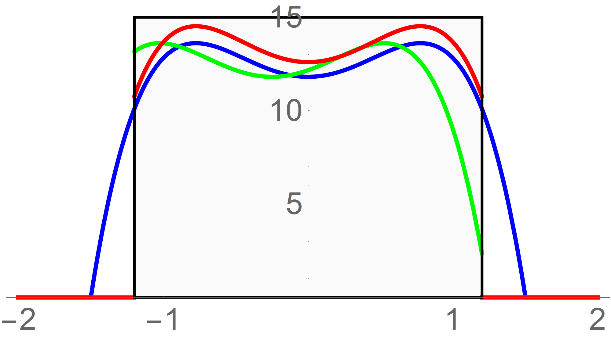
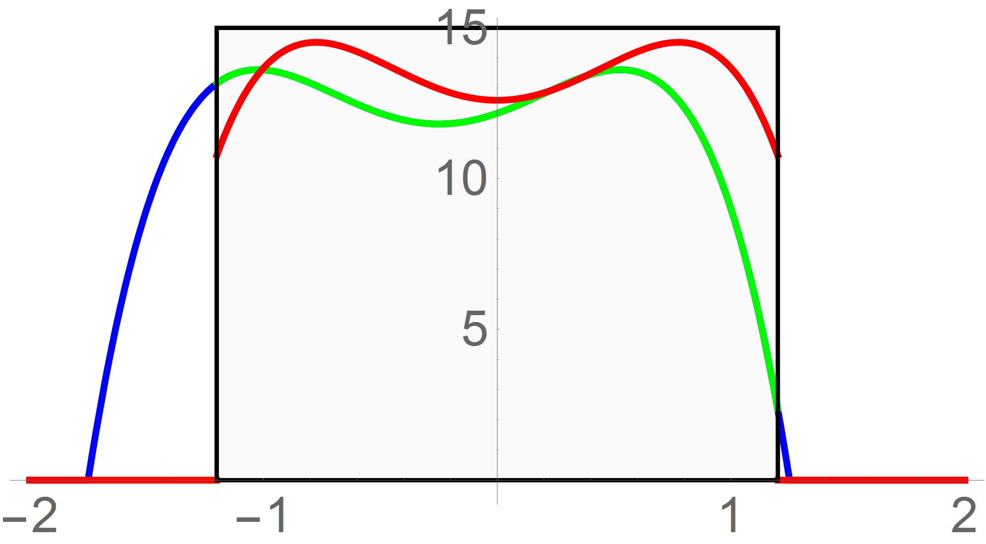
(a)	(b)

Figure 4: Toy example of signal matching through shift.

For visualization purpose, we replace the equality in (12) by a quadratic penalty. This encompasses both the objective and constraint into a single objective to be visualized. The resulted optimization landscape is shown in Figure 5. A local minimum is apparent around $c_{1}=0,\theta=0$ while the global minimum is around $c_{1}=1,\theta=0.25$.

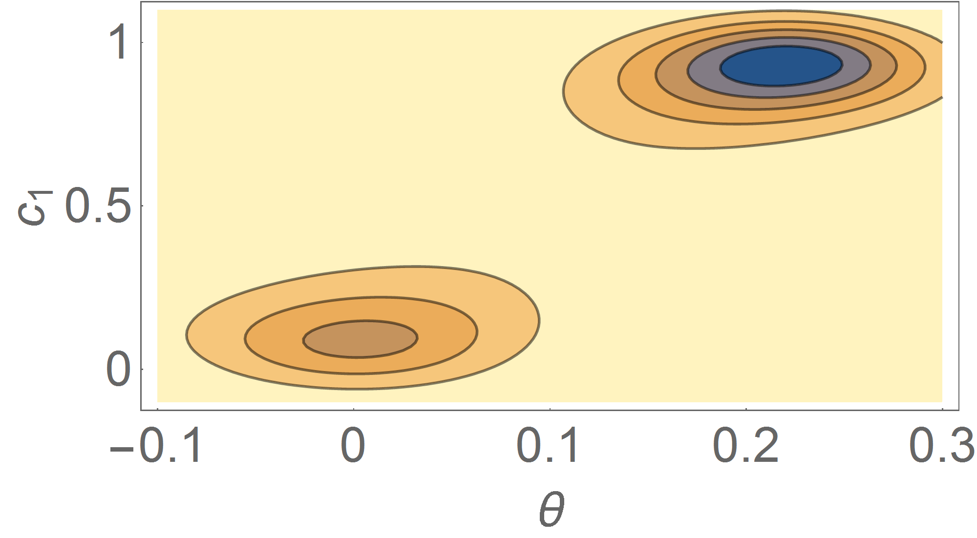
(a)	(b)

Figure 5: Objective landscape for the toy problem: signal matching through shift.

4 Diffusion

One way to approximate the solution of a nonconvex optimization problem is by diffusion and the continuation method. The idea is to follow the minimizer of the diffused cost function while progressively transforming that function to the original nonconvex cost. It has recently been shown that, this procedure with the choice of the heat kernel as the diffusion operator, provides the optimal transformation in a certain sense [Mobahi and Fisher III, 2015a]. In fact, some performance guarantees have been recently developed for this scheme [Mobahi and Fisher III, 2015b]. The procedure is defined more formally below. Given an unconstrained and nonconvex cost function $h:\mathbb{R}^{n}\rightarrow\mathbb{R}$ to be minimized. Instead of applying a local optimization algorithm directly to $h$, we embed $h$ into a family of functions parameterized by $\sigma$,

$$g(\boldsymbol{x}\,;\,\sigma)\triangleq[h\star k_{\sigma}](\boldsymbol{x})\,,$$ (13)

where $\star$ is the convolution operator and $k_{\sigma}(\boldsymbol{x})$ is the Gaussian function with zero mean and covariance $\sigma^{2}\boldsymbol{I}$. The Gaussian convolution appears here due to the known analytical solution form of the heat diffusion. Observe that $\lim_{\sigma\rightarrow\infty}g(\,.\,;\sigma)=h(\boldsymbol{x})$. Thus by starting from a large $\sigma$ and shrinking it toward zero, a sequence of cost function converging to $h$ is obtained. The optimization process then follows the path of the minimizer of $g(\,.\,;\sigma)$ through this sequence as listed in Algorithm 1.

Algorithm 1 Optimization by Diffusion and Continuation

1:  Input: $f:\mathcal{X}\rightarrow\mathbb{R}$, Sequence $\sigma_{0}>\sigma_{1}>\dots>\sigma_{n}=0$.

2:  $\boldsymbol{x}_{0}=$ global minimizer of $g(\boldsymbol{x};\sigma_{0})$.

3:  for $k=1$ to $n$ do

4:     $\boldsymbol{x}_{k}=$ Local minimizer of $g(\boldsymbol{x};\sigma_{k})$, initialized at $\boldsymbol{x}_{k-1}$.

5:  end for

6:  Output: $\boldsymbol{x}_{n}$

Now let us revisit the problem (12). Like before, we use a quadratic penalty to obtain an unconstrained approximate to (12). A sequence of diffused landscapes of this problem is shown in Figure 6. Note that the problem becomes convex, with a unique strict minimizer at the large $\sigma$. The solution path originated from that point eventually lands at the global minimum in this example.

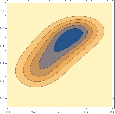
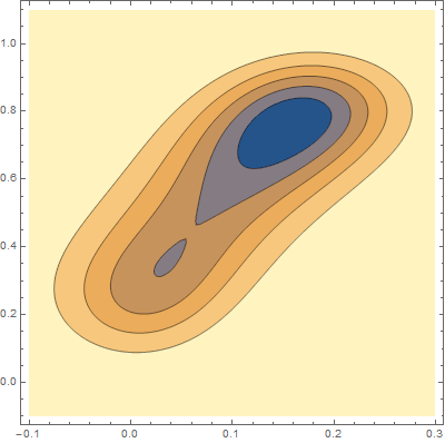
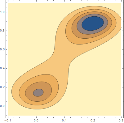
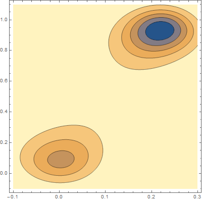
Figure 6: From left to right: diffused cost functions from a large $\sigma$ toward $\sigma=0$ for the toy example.

5 Deriving SIFT via the Diffusion Theory

Instead of pixel intensity as (11) to guide the matching, we switch to orientation of gradient. This change adds limited robustness to illumination changes [Dong and Soatto, 2015]. Nevertheless, the cost function remains nonconvex and difficult to minimize. Such nonconvex optimization may be treated via diffusion and continuation by the theory of [Mobahi and Fisher III, 2015a]. We show that SIFT descriptor emerges as an approximation to this process when $\tau$ is a similarity transformation, i.e. $\tau(\boldsymbol{x}\,;\,\boldsymbol{\theta})\triangleq e^{s}\boldsymbol{R}_{\alpha}\boldsymbol{x}+\boldsymbol{b}$, where $\boldsymbol{\theta}\triangleq(\alpha,s,\boldsymbol{b})$.

The approximation comes from two sources. First, the theory of [Mobahi and Fisher III, 2015a] suggests a continuation method by gradually reducing $\sigma$ while following the path of the minimizer. SIFT provides an approximation to this process by solving the optimization at only one value of $\sigma$, i.e. it terminates after the first iteration of the algorithm suggested by [Mobahi and Fisher III, 2015a]. Second, the cost function is diffused only w.r.t. a subset of optimization variables ($\alpha$ and $\boldsymbol{b}$). This deviates from the theory in [Mobahi and Fisher III, 2015a] that requires diffusion of the cost function in all variables, i.e. to use $[cost\star k_{\sigma}](\boldsymbol{c},\boldsymbol{\theta})$.

5.1 Energy Function

Define the density of gradient orientations of image $f$ as below,

$$h(\beta,\boldsymbol{x}\,;\,f)\triangleq\Sh(\angle\nabla f(\boldsymbol{x})-\beta)\,\|\nabla f(\boldsymbol{x})\|\,,$$ (14)

where denotes the Dirac comb of period $2\pi$, i.e. $\Sh(x)\triangleq\sum_{n=-\infty}^{\infty}\delta(x+2\pi n)$. The Dirac comb accounts for the periodicity of the angle (gradient orientation). Let the dissimilarity between a pair of density functions over a region $\mathcal{X}$ be expressed as the negated dot product,

$$d(f_{1},f_{2},\mathcal{X}) \triangleq -\int_{0}^{2\pi}\int_{\mathcal{X}}h(\beta,\boldsymbol{x}\,;\,f_{1})\,\,h(\beta,\boldsymbol{x}\,;\,f_{2})\,\,d\beta\,d\boldsymbol{x}\,.$$ (15)

In this setting, the problem of template matching is to find $\boldsymbol{\theta}$ such that the gradient orientations of $f(\tau(\boldsymbol{x}\,;\,\boldsymbol{\theta}))$ match that of a template,

$$(\boldsymbol{c}^{*},\boldsymbol{\theta}^{*})\triangleq\operatornamewithlimits{argmin}_{(\boldsymbol{c},\boldsymbol{\theta})}\sum_{k}c_{k}\,d(f\circ\tau_{\boldsymbol{\theta}},p_{k},\mathcal{X}_{k})$$

s.t $$\sum_{k}c_{k}=1\quad,\quad\forall k\,;\,c_{k}(1-c_{k})=0\,.$$ (16)

Replacing the equality constraint by some penalty function $q$ leads to the following unconstrained optimization,

$$cost(\boldsymbol{c},\boldsymbol{\theta})\triangleq q(\boldsymbol{c})\,+\,\sum_{k}c_{k}\,d(f\circ\tau_{\boldsymbol{\theta}},p_{k},\mathcal{X}_{k})\,.$$ (17)

5.2 Solution

1: Input: $\sigma_{0}>\sigma_{1}>\dots>\sigma_{n}=0$.

2: $(\boldsymbol{\theta}_{0},\boldsymbol{c}_{0})=\operatornamewithlimits{argmin}_{(\boldsymbol{\theta},\boldsymbol{c})}[cost\star k_{\sigma_{0}}](\boldsymbol{c},\boldsymbol{\theta})$.

3: for $k=1$ to $n$ do

4:    $(\boldsymbol{\theta}_{k},\boldsymbol{c}_{k})=$ Local min of $[cost\star k_{\sigma_{k}}](\boldsymbol{c},\boldsymbol{\theta})$, initialized at $(\boldsymbol{\theta}_{k-1},\boldsymbol{c}_{k-1})$.

5: end for

6: Output: $(\boldsymbol{\theta}_{n},\boldsymbol{c}_{n})$

1: Input: $\sigma_{0}$, $\Theta\triangleq\cup_{j}\{(\alpha_{j},s_{j},\boldsymbol{b}_{j})\}$.

2: $(\boldsymbol{\theta}_{0},\boldsymbol{c}_{0})=\operatornamewithlimits{argmin}_{(\boldsymbol{c},\alpha,s,\boldsymbol{b})}[cost(\boldsymbol{c},\,.\,s\,.\,)\star k_{\sigma_{0}}](\alpha,\boldsymbol{b})$ s.t. $(\alpha,s,\boldsymbol{b})\in\Theta$.

3: Output: $(\boldsymbol{\theta}_{0},\boldsymbol{c}_{0})$

1: Input: $\sigma_{0}$, $\Theta\triangleq\cup_{j}\{(\alpha_{j},s_{j},\boldsymbol{b}_{j})\}$.

2: $(j^{*},k^{*})=\operatornamewithlimits{argmax}_{j,k}\int_{0}^{2\pi}\int_{\mathcal{X}_{k}^{\dagger}}h(\beta,\boldsymbol{x}\,;\,p_{k})h_{SIFT}(\beta,\boldsymbol{x}\,,;\,f_{j})\,d\boldsymbol{x}\,d\beta$ s.t. $(\alpha,s,\boldsymbol{b})\in\Theta$.

3: Output: $(j^{*},k^{*})$

Table 2: Left: Ideal Minimization Strategy based on [Mobahi and Fisher III, 2015a]. Middle: Approximation due to a fixed $\sigma$ and partial diffusion. Right: Equivalence with SIFT up to the approximation (1).

The goal is to tackle the nonconvex problem (17) using the diffusion and continuation theory of [Mobahi and Fisher III, 2015a]. This would give the algorithm listed in Table 2-left.

SIFT based matching can be derived by simplifying this algorithm as described below,

• Partial Diffusion: Instead of diffusion w.r.t. all variables $(\alpha,s,\boldsymbol{b},\boldsymbol{c})$, diffuse the energy function (17) partially, i.e. only with respect to $(\alpha,\boldsymbol{b})$.

• Fixed $\sigma$: Instead of gradual refinement of the energy function by shrinking $\sigma$ toward zero, stick to a single choice $\sigma=\sigma_{0}$.

• Limited Optimization: Rather than searching the entire parameter space for $(\alpha,s,\boldsymbol{b})$ for the optimal solution, restrict to a small candidate set $\Theta\triangleq\cup_{j=1}^{J}\{(\alpha_{j},s_{j},\boldsymbol{b}_{j})\}$. This set is generated outside of the optimization loop by a keypoint detector. Consequently, $\Theta$ does not necessarily contain the optimal parameter as keypoint estimation is done for each image in isolation and thus separately from the full matching problem.

Applying these simplifications yields the algorithm in Table 2-middle. The central optimization in this algorithm is the following,

$$\min_{(\alpha,s,\boldsymbol{b})\in\Theta}\min_{\boldsymbol{c}}\big{[}\,[cost\big{(}\boldsymbol{c},(\,.\,,s,\,.\,)\big{)}\star k_{\sigma_{d}}](\boldsymbol{b})\,\star\tilde{k}_{\sigma_{r}}\,\big{]}(\alpha)\,,$$ (18)

where we have replaced the joint optimization $\min_{\boldsymbol{c},(\alpha,s,\boldsymbol{b})\in\Theta}$ by the equivalent nested form $\min_{(\alpha,s,\boldsymbol{b})\in\Theta}\min_{\boldsymbol{c}}$. The outer minimization is trivial; it just loops over the candidates and evaluates the resulted cost to pick the best one. Below we only focus on the inner optimization.

Assuming the penalty function $q(\boldsymbol{c})$ accurately enforces the constraint $c_{k}\in\{0,1\}$, the inner optimization becomes a winner take all problem; the winning patch $p_{k}$ to match $f$ is the one which minimizes the following cost,

$$k^{*} = \operatornamewithlimits{argmin}_{k}\big{[}\,[d(f\circ\tau_{(\,.\,,s,\,.\,)},p_{k},\mathcal{X}_{k})\star k_{\sigma_{d}}](\boldsymbol{b})\,\star\tilde{k}_{\sigma_{r}}\,\big{]}(\alpha)$$

$$= \operatornamewithlimits{argmax}_{k}\int_{0}^{2\pi}\int_{\mathcal{X}_{k}}\Big{(}\big{[}\,[h(\beta,\boldsymbol{x}\,;\,f\circ\tau_{(\,.\,,s,\,.\,)})\star k_{\sigma_{d}}](\boldsymbol{b})\,\star\tilde{k}_{\sigma_{r}}\,\big{]}(\alpha)\Big{)}\,\,h(\beta,\boldsymbol{x}\,;\,p_{k})\,\,d\beta\,d\boldsymbol{x}\,.$$

We doubt that the convolutions in (5.2) are computationally tractable. Thus, in order to derive a computationally tractable algorithm, we resort to a closed form approximation to the above convolutions. The approximation is stated in the following lemma.

Lemma 1

The following approximation holds,

$$\big{[}\,[h(\beta,\boldsymbol{x}\,;\,f\circ\tau_{(\,.\,,s,\,.\,)})\star k_{\sigma_{d}}](\boldsymbol{b})\,\star\tilde{k}_{\sigma_{r}}\,\big{]}(\alpha)$$

$$\approx \,-\,e^{s}\,\int_{\mathbb{R}^{2}}\tilde{k}_{\sigma_{r}}(\angle\nabla f(\boldsymbol{y})-\alpha-\beta)\|\nabla f(\boldsymbol{y})\|\,k_{\sigma_{d}}(\boldsymbol{y}-e^{s}\boldsymbol{R}_{\alpha}\boldsymbol{x}-\boldsymbol{b})\,d\boldsymbol{y}\,.$$

• See Appendix B for the proof.

Using this lemma, the computationally intractable optimization (18) is replaced by the following tractable approximation,

$$\max_{(\alpha,s,\boldsymbol{b})\in\Theta}\max_{k}\,e^{s}\,\int_{0}^{2\pi}\int_{\mathcal{X}_{k}}\int_{\mathbb{R}^{2}}\tilde{k}_{\sigma_{r}}(\angle\nabla f(\boldsymbol{y})-\alpha-\beta)\|\nabla f(\boldsymbol{y})\|\,k_{\sigma_{d}}(\boldsymbol{y}-e^{s}\boldsymbol{R}_{\alpha}\boldsymbol{x}-\boldsymbol{b})\,d\boldsymbol{y}$$

$$\hskip 130.08621pt\times h(\beta,\boldsymbol{x}\,;\,p_{k})\,d\boldsymbol{x}\,d\beta\,,$$ (20)

In the inner optimization, since $(\alpha,s,\boldsymbol{b})$ is fixed (to some $(\alpha_{j},s_{j},\boldsymbol{b}_{j})$), the image $f$ can be warped prior to optimization by $\tau(\,.\,;\alpha_{j},s_{j},\boldsymbol{b}_{j})$. This allows optimization w.r.t. $k$ to be performed for $\tau$ being the identity transform (because the effect of $(\alpha_{j},s_{j},\boldsymbol{b}_{j})$ is already taken care of by the warp), i.e. $(\alpha=0,s=0,\boldsymbol{b}=\boldsymbol{0})$. Denoting the warped $f$ due to $(\alpha_{j},s_{j},\boldsymbol{b}_{j})$ by $f_{j}\triangleq f\circ\tau_{\boldsymbol{\theta}_{j}}$, the inner optimization simplifies,

$$\max_{k}\,\int_{0}^{2\pi}\int_{\mathcal{X}_{k}}\underbrace{\int_{\mathbb{R}^{2}}\tilde{k}_{\sigma_{r}}(\angle\nabla f_{j}(\boldsymbol{y})-\beta)\|\nabla f_{j}(\boldsymbol{y})\|\,k_{\sigma_{d}}(\boldsymbol{y}-\boldsymbol{x})\,d\boldsymbol{y}}_{h_{SIFT}(\beta,\boldsymbol{x}\,;\,f_{j})}\,h(\beta,\boldsymbol{x}\,;\,p_{k})\,d\boldsymbol{x}\,d\beta\,,$$ (21)

Part of the computation involving $f_{j}$ is independent of $p_{k}$ and can be precomputed. This precomputed result in fact provides a new representation for $f_{j}$ that matches the definition of $h_{SIFT}$ in (2). This gives the algorithm presented in Table 2-Right.

6 Deriving DSP-SIFT via the Diffusion Theory

Here we show that the DSP-SIFT descriptor also relates to partial diffusion of the cost function. Specifically, this descriptor can be derived by considering the diffusion w.r.t. the transformation parameters $(\alpha,s,\boldsymbol{b})$. Note that this involves more of the optimization variables in diffusion compared to SIFT (which diffuses w.r.t. $(\alpha,\boldsymbol{b})$), and thus provides a better approximation to the theory of [Mobahi and Fisher III, 2015a] which suggests the diffusion must be applied to all optimization variables, i.e. to $(\boldsymbol{c},\boldsymbol{\theta})$. This improvement in approximation fidelity could be an explanation of why DSP-SIFT works better than SIFT in practice. However, it still misses diffusion of $\boldsymbol{c}$.

The derivation is quite similar to that of SIFT in Section 5. The is to minimize the same energy function in (17). However, on top of diffusion w.r.t. variables $(\alpha,\boldsymbol{b})$ we add a Gaussian convolution in $s$. By linearity of convolution, we can just take the diffused energy we obtained in (5.2) and put it under the Gaussian convolution in $s$. This leads to the following expression,

$$\max_{(\alpha,s,\boldsymbol{b})\in\Theta}\max_{k}\int_{0}^{2\pi}\int_{\mathcal{X}_{k}}\int_{\mathbb{R}^{2}}[\Big{(}\,e^{\,.\,}\,\tilde{k}_{\sigma_{r}}(\angle\nabla f(\boldsymbol{y})-\alpha-\beta)\|\nabla f(\boldsymbol{y})\|\,k_{\sigma_{d}}(\boldsymbol{y}-e^{\,.\,}\boldsymbol{R}_{\alpha}\boldsymbol{x}-\boldsymbol{b})$$

$$\hskip 130.08621pt\Big{)}\star k_{\sigma_{s}}](s)\,\,\,d\boldsymbol{y}\,h(\beta,\boldsymbol{x}\,;\,p_{k})\,d\boldsymbol{x}\,d\beta\,.$$ (22)

7 Implication for Future Algorithms

7.1 Closed Form Approximations for Domain Size Pooling

In DSP-SIFT, pooling over the scale is done numerically via sampling [Dong and Soatto, 2015]. Our theory suggests that the scale pooling should also be performed by Gaussian convolution, i.e. (6). Using this form, we present a closed-form approximation, which consequently does not require any sampling. Whether or not this approximation provides a satisfactory fidelity must be investigated by experiments.

Recall energy minimization formulation of DSP-SIFT (6) has the following form,

$$\max_{(\alpha,s,\boldsymbol{b})\in\Theta}\max_{k}\int_{0}^{2\pi}\int_{\mathcal{X}_{k}}\int_{\mathbb{R}^{2}}\Big{(}[\big{(}\,e^{\,.\,}\,\,k_{\sigma_{d}}(\boldsymbol{y}-e^{\,.\,}\boldsymbol{R}_{\alpha}\boldsymbol{x}-\boldsymbol{b})\big{)}\star k_{\sigma_{s}}](s)\Big{)}$$

$$\hskip 115.63243pt\,\tilde{k}_{\sigma_{r}}(\angle\nabla f(\boldsymbol{y})-\alpha-\beta)\|\nabla f(\boldsymbol{y})\|\,\,\,d\boldsymbol{y}\,h(\beta,\boldsymbol{x}\,;\,p_{k})\,d\boldsymbol{x}\,d\beta\,.$$ (23)

This convolution does not have a closed form. However, we consider approximating $e^{s}$ by its linearized form around $s=0$ (identity scaling transform), i.e. $e^{s}\approx 1+s$. Then the convolution will have a closed form. Below we present two approximation based on this idea.

Linearizing only the inner $e^{s}$

:

Proposition 2

$$[\Big{(}e^{\,.\,}\,k_{\sigma_{d}}(\boldsymbol{y}-(1+{\,.\,})\boldsymbol{R}_{\alpha}\boldsymbol{x}-\boldsymbol{b})\Big{)}\star k_{\sigma_{s}}](s)$$

$$= k_{\sigma_{d}}(\boldsymbol{y}-\boldsymbol{R}_{\alpha}\boldsymbol{x}-\boldsymbol{b})$$

$$\times k^{-1}_{\frac{\sigma_{d}}{\|\boldsymbol{x}\|}}(1+\frac{(\boldsymbol{R}_{\alpha}\boldsymbol{x})^{T}(\boldsymbol{b}-\boldsymbol{y})-\sigma_{d}^{2}}{\|\boldsymbol{x}\|^{2}})\times k_{\sqrt{\sigma_{s}^{2}+\frac{\sigma_{d}^{2}}{\|\boldsymbol{x}\|^{2}}}}(s+1+\frac{(\boldsymbol{R}_{\alpha}\boldsymbol{x})^{T}(\boldsymbol{b}-\boldsymbol{y})-\sigma_{d}^{2}}{\|\boldsymbol{x}\|^{2}})\,.$$

See Appendix A for the proof.

In particular, when the region is already warped, we can set $(\alpha,s,\boldsymbol{b})=(0,0,\boldsymbol{0})$. This allows the template matching solution (7.1) as below,

$\displaystyle\max_{j,k}\int_{0}^{2\pi}\int_{\mathcal{X}_{k}}\int_{\mathbb{R}^{2}}k_{\sigma_{d}}(\boldsymbol{y}-\boldsymbol{x})\times k^{-1}_{\frac{\sigma_{d}}{\|\boldsymbol{x}\|}}(1-\frac{\boldsymbol{x}^{T}\boldsymbol{y}+\sigma_{d}^{2}}{\|\boldsymbol{x}\|^{2}})\times k_{\sqrt{\sigma_{s}^{2}+\frac{\sigma_{d}^{2}}{\|\boldsymbol{x}\|^{2}}}}(1-\frac{\boldsymbol{x}^{T}\boldsymbol{y}+\sigma_{d}^{2}}{\|\boldsymbol{x}\|^{2}})$ $\displaystyle\hskip 72.26999pt\times\,\tilde{k}_{\sigma_{r}}(\angle\nabla f_{j}(\boldsymbol{y})-\beta)\|\nabla f_{j}(\boldsymbol{y})\|\,\,\,d\boldsymbol{y}\,h(\beta,\boldsymbol{x}\,;\,p_{k})\,d\boldsymbol{x}\,d\beta\,.$ (24)

Linearizing both the inner and outer $e^{s}$

:

We use the following identity,

$$[(1+\,.\,)k_{\sigma}(\boldsymbol{y}+(1+\,.\,)\boldsymbol{x})\star k_{scale}](s)$$ (25)

$$= \frac{\sigma^{2}(1+s)-\sigma_{scale}\boldsymbol{x}^{T}\boldsymbol{y}}{2\pi\sigma(\sigma^{2}+\sigma_{scale}^{2}\|\boldsymbol{x}\|^{2})^{\frac{3}{2}}}e^{-\frac{\sigma^{2}\|(1+s)\boldsymbol{x}+\boldsymbol{y}\|^{2}+\sigma_{scale}^{2}(\boldsymbol{x}^{T}\boldsymbol{y}^{\perp})^{2}}{2\sigma^{2}(\sigma^{2}+\sigma_{scale}^{2}\|\boldsymbol{x}\|^{2})}}$$ (26)

Thus,

$$[(1+\,.\,)k_{\sigma_{d}}(\boldsymbol{y}-\boldsymbol{b}-(1+\,.\,)\boldsymbol{R}_{\alpha}\,\boldsymbol{x})\star k_{\sigma_{s}}](s)$$ (27)

$$= \frac{\sigma_{d}^{2}(1+s)+\sigma_{s}\boldsymbol{x}^{T}\boldsymbol{R}^{T}_{\alpha}(\boldsymbol{y}-\boldsymbol{b})}{2\pi\sigma_{d}(\sigma_{d}^{2}+\sigma_{s}^{2}\|\boldsymbol{x}\|^{2})^{\frac{3}{2}}}e^{-\frac{\sigma_{d}^{2}\|-(1+s)\boldsymbol{R}_{\alpha}\boldsymbol{x}+\boldsymbol{y}-\boldsymbol{b}\|^{2}+\sigma_{s}^{2}((\boldsymbol{R}_{\alpha}\boldsymbol{x})^{T}(\boldsymbol{y}-\boldsymbol{b})^{\perp})^{2}}{2\sigma_{d}^{2}(\sigma_{d}^{2}+\sigma_{s}^{2}\|\boldsymbol{x}\|^{2})}}\,.$$ (28)

In particular, when the region is already warped, we can set $(\alpha,s,\boldsymbol{b})=(0,0,\boldsymbol{0})$. This allows the template matching solution (7.1) as below,

$\displaystyle\max_{j,k}\int_{0}^{2\pi}\int_{\mathcal{X}_{k}}\int_{\mathbb{R}^{2}}\frac{\sigma_{d}^{2}+\sigma_{s}\boldsymbol{x}^{T}\boldsymbol{y}}{(\sigma_{d}^{2}+\sigma_{s}^{2}\|\boldsymbol{x}\|^{2})^{\frac{3}{2}}}e^{-\frac{\sigma_{d}^{2}\|\boldsymbol{y}-\boldsymbol{x}\|^{2}+\sigma_{s}^{2}(\boldsymbol{x}^{T}\boldsymbol{y}^{\perp})^{2}}{2\sigma_{d}^{2}(\sigma_{d}^{2}+\sigma_{s}^{2}\|\boldsymbol{x}\|^{2})}}$ (29) $\displaystyle\hskip 72.26999pt\times\,\tilde{k}_{\sigma_{r}}(\angle\nabla f_{j}(\boldsymbol{y})-\beta)\|\nabla f_{j}(\boldsymbol{y})\|\,\,\,d\boldsymbol{y}\,h(\beta,\boldsymbol{x}\,;\,p_{k})\,d\boldsymbol{x}\,d\beta\,.$ (30)

7.2 Exact Diffusion for Affine Transform

Using the diffusion theory, by using a different parameterization for the geometric transformation, we can potentially improved SIFT and DSP-SIFT in two ways.

1. We can extend the descriptor from handling similarity transform to affine transform.

2. Recall that the computation of the diffusion in SIFT and DSP-SIFT relies on some approximation. In addition, regardless of the diffusion theory, DSP-SIFT involves sampling to approximate one of the required integrals. The finite sampling process is inaccurate and expensive to compute. Here despite working with a larger transformation space, the new parameterization allows deriving exact and closed form expression for the diffusion in all transformation parameters.

The formulation of the energy function is similar to that of SIFT and DSP-SIFT, except the parameterization. Instead of the similarity transform $\boldsymbol{\tau}$ as $\tau(\boldsymbol{x}\,;\,\alpha,s,\boldsymbol{b})\triangleq e^{s}\boldsymbol{R}_{\alpha}\boldsymbol{x}+\boldsymbol{b}$ we switch to the affine transform $\tau(\boldsymbol{x}\,;\,\boldsymbol{A},\boldsymbol{b})\triangleq\boldsymbol{A}\boldsymbol{x}+\boldsymbol{b}$, as listed below,

$$cost(\boldsymbol{c},\boldsymbol{A},\boldsymbol{b})\triangleq q(\boldsymbol{c})\,+\,\sum_{k}c_{k}\,d(f\circ\tau_{\boldsymbol{A},\boldsymbol{b}},p_{k},\mathcal{X}_{k})\,,$$ (31)

where the dissimilarity functional $d$ is defined as earlier in (15). Recall that the goal is to tackle the nonconvex problem (31) using the diffusion theory of [Mobahi and Fisher III, 2015a] and similar simplifications as in Section 5, we obtain the following solution for the template matching problem.

$$k^{*} = \operatornamewithlimits{argmin}_{k}\big{[}\,[d(f\circ\tau_{(\,.\,,\,.\,)},p_{k},\mathcal{X}_{k})\star k_{\sigma_{b}}](\boldsymbol{b})\,\star\tilde{k}_{\sigma_{a}}\,\big{]}(\boldsymbol{A})$$

$$= \operatornamewithlimits{argmax}_{k}\int_{0}^{2\pi}\int_{\mathcal{X}_{k}}\Big{(}\big{[}\,[h(\beta,\boldsymbol{x}\,;\,f\circ\tau_{(\,.\,,\,.\,)})\star k_{\sigma_{b}}](\boldsymbol{b})\,\star\tilde{k}_{\sigma_{a}}\,\big{]}(\boldsymbol{A})\Big{)}\,\,h(\beta,\boldsymbol{x}\,;\,p_{k})\,\,d\beta\,d\boldsymbol{x}\,.$$

Interesting, we can replace the above convolutions by a closed form and exact expression. This is stated in the following lemma.

Lemma 3

$$\big{[}\big{(}[h(\beta,\boldsymbol{x}\,;\,f\circ\tau_{(\,.\,,\,.\,)})\star k_{\sigma_{b}}](\boldsymbol{b})\big{)}\star k_{\sigma_{a}}\big{]}(\boldsymbol{A})$$

$$= \frac{e^{-\frac{((\boldsymbol{b}-\boldsymbol{y})^{T}\tilde{\nabla}f(\boldsymbol{y}))^{2}}{2\sigma_{b}^{2}}-\frac{\|\boldsymbol{A}^{T}\tilde{\nabla}f(\boldsymbol{y})\|^{2}}{2{\sigma_{a}}^{2}}}w(-\frac{\sigma_{b}^{-2}\tilde{\nabla}^{T}f(\boldsymbol{y})(\boldsymbol{y}-\boldsymbol{b})\boldsymbol{x}^{T}\tilde{\boldsymbol{v}}(\beta,\boldsymbol{y})+{\sigma_{a}}^{-2}\tilde{\nabla}^{T}f(\boldsymbol{y})\boldsymbol{A}\tilde{\boldsymbol{v}}(\beta,\boldsymbol{y})}{2t})}{8\sqrt{2}\pi^{\frac{3}{2}}\sigma_{b}{\sigma_{a}}^{2}\,\|\nabla f(\boldsymbol{y})\|^{2}\,t^{3}}\,,$$

where $\tilde{\nabla}f(\boldsymbol{y})\triangleq\frac{\nabla f(\boldsymbol{y})}{\|\nabla f(\boldsymbol{y})\|}$, $\tilde{\boldsymbol{v}}(\beta,\boldsymbol{y})\triangleq\frac{\boldsymbol{v}(\beta)}{\|\nabla f(\boldsymbol{y})\|}$, and $t\triangleq\sqrt{\frac{(\boldsymbol{x}^{T}\tilde{\boldsymbol{v}}(\beta,\boldsymbol{y}))^{2}}{2\sigma_{b}^{2}}+\frac{1}{2{\sigma_{a}}^{2}\,\|\nabla f(\boldsymbol{y})\|^{2}}}$ and $w(x)\triangleq\sqrt{\pi}e^{x^{2}}(1+2x^{2})\operatorname{erfc}(x)-2x$.

• See Appendix C for the proof.

Similar to the arguments about SIFT solution in Section 5, the inner optimization in (7.2) can work with the warped $f$ so that the transformation $\tau(\boldsymbol{x}\,;\,\boldsymbol{A},\boldsymbol{b})$ simplifies to the identity transform $(\boldsymbol{A}=\boldsymbol{I},\boldsymbol{b}=\boldsymbol{0})$. Letting the warped $f$ be $f_{j}\triangleq f\circ\tau_{\boldsymbol{A}_{j},\boldsymbol{b}_{j}}$, the inner optimization simplifies,

where $h_{heat}$ is defined as the result in lemma 2 (diffused $h$) with $(\boldsymbol{A}=\boldsymbol{I},\boldsymbol{b}=\boldsymbol{0})$, $\sigma_{a}$ and $\sigma_{b}$ fixed, and all constants dropped,

$\displaystyle(j^{*},k^{*})$ $\displaystyle\triangleq$ $\displaystyle\operatornamewithlimits{argmax}_{j,k}\,\int_{0}^{2\pi}\int_{\mathcal{X}_{k}}h_{heat}(\beta,\boldsymbol{x}\,;\,f_{j})\,h(\beta,\boldsymbol{x}\,;\,p_{k})\,d\boldsymbol{x}\,d\beta$ $\displaystyle h_{heat}(\beta,\boldsymbol{x}\,;\,f)$ $\displaystyle\triangleq$ $\displaystyle\frac{e^{-\frac{(\boldsymbol{y}^{T}\tilde{\nabla}f(\boldsymbol{y}))^{2}}{2\sigma_{b}^{2}}}w\big{(}-\frac{1}{2t}\,\tilde{\nabla}^{T}f(\boldsymbol{y})\,(\,\sigma_{b}^{-2}\,\boldsymbol{y}\boldsymbol{x}^{T}\,+\,{\sigma_{a}}^{-2}\,\boldsymbol{I}\,\big{)}\,\tilde{\boldsymbol{v}}(\beta,\boldsymbol{y})\big{)}}{\|\nabla f(\boldsymbol{y})\|^{2}\,t^{3}}$ $\displaystyle\tilde{\nabla}f(\boldsymbol{y})$ $\displaystyle\triangleq$ $\displaystyle\frac{\nabla f(\boldsymbol{y})}{\|\nabla f(\boldsymbol{y})\|}$ $\displaystyle\tilde{\boldsymbol{v}}(\beta,\boldsymbol{y})$ $\displaystyle\triangleq$ $\displaystyle\frac{\boldsymbol{v}(\beta)}{\|\nabla f(\boldsymbol{y})\|}$ $\displaystyle t$ $\displaystyle\triangleq$ $\displaystyle\sqrt{\frac{(\boldsymbol{x}^{T}\tilde{\boldsymbol{v}}(\beta,\boldsymbol{y}))^{2}}{2\sigma_{b}^{2}}+\frac{1}{2{\sigma_{a}}^{2}\,\|\nabla f(\boldsymbol{y})\|^{2}}}$ $\displaystyle w(x)$ $\displaystyle\triangleq$ $\displaystyle\sqrt{\pi}e^{x^{2}}(1+2x^{2})\operatorname{erfc}(x)-2x\,.$

Appendix

Appendix A Proof of Proposition 1

We proceed with the following identity,

$$e^{s}\times k_{\sigma}(\boldsymbol{y}-(1+s)\boldsymbol{R}_{\alpha}\boldsymbol{x}-\boldsymbol{b})$$ (35)

$$= k_{\sigma}(\boldsymbol{y}-\boldsymbol{R}_{\alpha}\boldsymbol{x}-\boldsymbol{b})\times k^{-1}_{\frac{\sigma}{\|\boldsymbol{R}_{\alpha}\boldsymbol{x}\|}}(1+\frac{(\boldsymbol{R}_{\alpha}\boldsymbol{x})^{T}(\boldsymbol{b}-\boldsymbol{y})-\sigma^{2}}{\|\boldsymbol{R}_{\alpha}\boldsymbol{x}\|^{2}})\times k_{\frac{\sigma}{\|\boldsymbol{R}_{\alpha}\boldsymbol{x}\|}}(s+1+\frac{(\boldsymbol{R}_{\alpha}\boldsymbol{x})^{T}(\boldsymbol{b}-\boldsymbol{y})-\sigma^{2}}{\|\boldsymbol{R}_{\alpha}\boldsymbol{x}\|^{2}})$$ (36)

$$= k_{\sigma}(\boldsymbol{y}-\boldsymbol{R}_{\alpha}\boldsymbol{x}-\boldsymbol{b})\times k^{-1}_{\frac{\sigma}{\|\boldsymbol{x}\|}}(1+\frac{(\boldsymbol{R}_{\alpha}\boldsymbol{x})^{T}(\boldsymbol{b}-\boldsymbol{y})-\sigma^{2}}{\|\boldsymbol{x}\|^{2}})\times k_{\frac{\sigma}{\|\boldsymbol{x}\|}}(s+1+\frac{(\boldsymbol{R}_{\alpha}\boldsymbol{x})^{T}(\boldsymbol{b}-\boldsymbol{y})-\sigma^{2}}{\|\boldsymbol{x}\|^{2}})$$ (37)

In this form, it is now very easy to compute convolution with $k_{\sigma_{{scale}}}(s)$,

$$[e^{\,.\,}\times k_{\sigma}(\boldsymbol{y}-(1+\,.\,)\boldsymbol{R}_{\alpha}\boldsymbol{x}-\boldsymbol{b})\star k_{\sigma_{{scale}}}](s)$$ (39)

$$= k_{\sigma}(\boldsymbol{y}-\boldsymbol{R}_{\alpha}\boldsymbol{x}-\boldsymbol{b})\times k^{-1}_{\frac{\sigma}{\|\boldsymbol{x}\|}}(1+\frac{(\boldsymbol{R}_{\alpha}\boldsymbol{x})^{T}(\boldsymbol{b}-\boldsymbol{y})-\sigma^{2}}{\|\boldsymbol{x}\|^{2}})\times k_{\sqrt{\sigma^{2}_{{scale}}+\frac{\sigma^{2}}{\|\boldsymbol{x}\|^{2}}}}(s+1+\frac{(\boldsymbol{R}_{\alpha}\boldsymbol{x})^{T}(\boldsymbol{b}-\boldsymbol{y})-\sigma^{2}}{\|\boldsymbol{x}\|^{2}})$$ (40)

Therefore,

$$[\Big{(}e^{\,.\,}\int_{\mathbb{R}^{2}}\tilde{k}_{\tilde{\sigma}}(\angle\nabla f(\boldsymbol{y})-\alpha-\beta)\|\nabla f(\boldsymbol{y})\|\,k_{\sigma}(\boldsymbol{y}-(1+{\,.\,})\boldsymbol{R}_{\alpha}\boldsymbol{x}-\boldsymbol{b})\,d\boldsymbol{y}\Big{)}\star k_{\sigma_{{scale}}}](s)$$ (42)

$$= \int_{\mathbb{R}^{2}}\tilde{k}_{\tilde{\sigma}}(\angle\nabla f(\boldsymbol{y})-\alpha-\beta)\|\nabla f(\boldsymbol{y})\|\,k_{\sigma}(\boldsymbol{y}-\boldsymbol{R}_{\alpha}\boldsymbol{x}-\boldsymbol{b})$$

$$\times k^{-1}_{\frac{\sigma}{\|\boldsymbol{x}\|}}(1+\frac{(\boldsymbol{R}_{\alpha}\boldsymbol{x})^{T}(\boldsymbol{b}-\boldsymbol{y})-\sigma^{2}}{\|\boldsymbol{x}\|^{2}})\times k_{\sqrt{\sigma^{2}_{{scale}}+\frac{\sigma^{2}}{\|\boldsymbol{x}\|^{2}}}}(s+1+\frac{(\boldsymbol{R}_{\alpha}\boldsymbol{x})^{T}(\boldsymbol{b}-\boldsymbol{y})-\sigma^{2}}{\|\boldsymbol{x}\|^{2}})\,d\boldsymbol{y}\,.$$

Appendix B Proof of Lemma 1

$$cost(\boldsymbol{c},\boldsymbol{\theta})$$ (44)

$$\triangleq q(\boldsymbol{c})\,+\,\sum_{k}c_{k}\,d(f\circ\tau_{(\alpha\,,s,\,\boldsymbol{b}\,)},p_{k},\mathcal{X}_{k})$$ (45)

$$= q(\boldsymbol{c})\,+\,\sum_{k}c_{k}\,\int_{0}^{2\pi}\Big{(}h(\beta\,;\,f\circ\tau_{(\alpha,s,\,\boldsymbol{b}\,)},\mathcal{X}_{k})-h(\beta\,;\,p_{k},\mathcal{X}_{k})\Big{)}^{2}\,d\beta\,.$$ (46)

Note that,

$$h(\beta\,;\,f\circ\tau_{(\alpha,s,\,\boldsymbol{b}\,)},\mathcal{X}_{k})$$ (47)

$$= \int_{\mathcal{X}_{k}}\Sh(\angle\nabla(f(e^{s}\boldsymbol{R}_{\alpha}\boldsymbol{x}+\boldsymbol{b}))-\beta)\|\nabla f(e^{s}\boldsymbol{R}_{\alpha}\boldsymbol{x}+\boldsymbol{b})\|\,d\boldsymbol{x}$$ (48)

$$= \int_{\mathcal{X}_{k}}\Sh(\angle e^{s}\boldsymbol{R}^{T}_{\alpha}[\nabla f](e^{s}\boldsymbol{R}_{\alpha}\boldsymbol{x}+\boldsymbol{b})-\beta)\|e^{s}\boldsymbol{R}^{T}_{\alpha}\nabla f(e^{s}\boldsymbol{R}_{\alpha}\boldsymbol{x}+\boldsymbol{b})\|\,d\boldsymbol{x}$$ (49)

$$= \int_{\mathcal{X}_{k}}\Sh(\angle\nabla f(e^{s}\boldsymbol{R}_{\alpha}\boldsymbol{x}+\boldsymbol{b})-\alpha-\beta)e^{s}\|\nabla f(e^{s}\boldsymbol{R}_{\alpha}\boldsymbol{x}+\boldsymbol{b})\|\,d\boldsymbol{x}\,,$$ (50)

where (49) uses the chain rule of derivative $\nabla\big{(}f(\boldsymbol{Ax}+\boldsymbol{b})\big{)}=\boldsymbol{A}^{T}\big{(}[\nabla f](\boldsymbol{Ax}+\boldsymbol{b})\big{)}$. Also, for any $a>0$, (50) uses the identities $\|a\boldsymbol{R}\boldsymbol{x}\|=a\|\boldsymbol{x}\|$ and $\angle a\boldsymbol{R}_{\alpha}\boldsymbol{x}=\alpha+\angle\boldsymbol{x}$. Thus, it follows that,

$$cost(\boldsymbol{c},\boldsymbol{\theta})$$ (51)

$$= q(\boldsymbol{c})\,+\,\sum_{k}c_{k}\,\int_{0}^{2\pi}\Big{(}\int_{\mathcal{X}_{k}}\Sh(\angle\nabla f(e^{s}\boldsymbol{R}_{\alpha}\boldsymbol{x}+\boldsymbol{b})-\alpha-\beta)e^{s}\|\nabla f(e^{s}\boldsymbol{R}_{\alpha}\boldsymbol{x}+\boldsymbol{b})\|\,d\boldsymbol{x}-h(\beta\,;\,p_{k},\mathcal{X}_{k})\Big{)}^{2}\,d\beta\,.$$ (52)

By the linearity of the convolution operator and the unity of Gaussian’s total mass, smoothed $cost$ amounts only to replacing $\Big{(}\int_{\mathcal{X}_{k}}\Sh(\angle\nabla f(e^{s}\boldsymbol{R}_{\alpha}\boldsymbol{x}+\boldsymbol{b})-\alpha-\beta)e^{s}\|\nabla f(e^{s}\boldsymbol{R}_{\alpha}\boldsymbol{x}+\boldsymbol{b})\|\,d\boldsymbol{x}-h(\beta\,;\,p_{k},\mathcal{X}_{k})\Big{)}^{2}$ by its smoothed version. Expansion of the quadratic form yields,

$$\Big{(}\int_{\mathcal{X}_{k}}\Sh(\angle\nabla f(e^{s}\boldsymbol{R}_{\alpha}\boldsymbol{x}+\boldsymbol{b})-\alpha-\beta)e^{s}\|\nabla f(e^{s}\boldsymbol{R}_{\alpha}\boldsymbol{x}+\boldsymbol{b})\|\,d\boldsymbol{x}-h(\beta\,;\,p_{k},\mathcal{X}_{k})\Big{)}^{2}$$ (53)

$$= \Big{(}\int_{\mathcal{X}_{k}}\Sh(\angle\nabla f(e^{s}\boldsymbol{R}_{\alpha}\boldsymbol{x}+\boldsymbol{b})-\alpha-\beta)e^{s}\|\nabla f(e^{s}\boldsymbol{R}_{\alpha}\boldsymbol{x}+\boldsymbol{b})\|\,d\boldsymbol{x}\Big{)}^{2}+h^{2}(\beta\,;\,p_{k},\mathcal{X}_{k})$$ (55)

$$-2\Big{(}\int_{\mathcal{X}_{k}}\Sh(\angle\nabla f(e^{s}\boldsymbol{R}_{\alpha}\boldsymbol{x}+\boldsymbol{b})-\alpha-\beta)e^{s}\|\nabla f(e^{s}\boldsymbol{R}_{\alpha}\boldsymbol{x}+\boldsymbol{b})\|\,d\boldsymbol{x}\Big{)}\times h(\beta\,;\,p_{k},\mathcal{X}_{k})\,.$$

The first term can be rewritten as below,

$$\Big{(}\int_{\mathcal{X}_{k}}\Sh(\angle\nabla f(e^{s}\boldsymbol{R}_{\alpha}\boldsymbol{x}+\boldsymbol{b})-\alpha-\beta)e^{s}\|\nabla f(e^{s}\boldsymbol{R}_{\alpha}\boldsymbol{x}+\boldsymbol{b})\|\,d\boldsymbol{x}\Big{)}^{2}$$ (56)

$$= e^{2s}\int_{\mathcal{X}_{k}}\,\,|\{\boldsymbol{x}_{2}\,|\,\angle\nabla f(e^{s}\boldsymbol{R}_{\alpha}\boldsymbol{x}_{2}+\boldsymbol{b})=\angle\nabla f(e^{s}\boldsymbol{R}_{\alpha}\boldsymbol{x}+\boldsymbol{b})\}|$$ (58)

$$\times\Sh(\angle\nabla f(e^{s}\boldsymbol{R}_{\alpha}\boldsymbol{x}+\boldsymbol{b})-\alpha-\beta)\,\|\nabla f(e^{s}\boldsymbol{R}_{\alpha}\boldsymbol{x}+\boldsymbol{b})\|^{2}\,d\boldsymbol{x}\,.$$

Note that $|\{\boldsymbol{x}_{2}\,|\,\angle\nabla f(e^{s}\boldsymbol{R}_{\alpha}\boldsymbol{x}_{2}+\boldsymbol{b})=\angle\nabla f(e^{s}\boldsymbol{R}_{\alpha}\boldsymbol{x}+\boldsymbol{b})\}|\geq 1$ because at least there is one such $\boldsymbol{x}_{2}$ for which $\angle\nabla f(e^{s}\boldsymbol{R}_{\alpha}\boldsymbol{x}_{2}+\boldsymbol{b})=\angle\nabla f(e^{s}\boldsymbol{R}_{\alpha}\boldsymbol{x}+\boldsymbol{b})$ holds, that is $\boldsymbol{x}_{2}=\boldsymbol{x}$. However, we assume that the cardinality of the set is exactly one, i.e. besides $\boldsymbol{x}_{2}=\boldsymbol{x}$, there is no other choice for $\boldsymbol{x}_{2}$ so that the condition $\angle\nabla f(e^{s}\boldsymbol{R}_{\alpha}\boldsymbol{x}_{2}+\boldsymbol{b})=\angle\nabla f(e^{s}\boldsymbol{R}_{\alpha}\boldsymbol{x}+\boldsymbol{b})$ can hold. The rationale is that the variables are continuous and thus their representation has infinite precision. The odds that the gradient orientation at two different points in the image are exactly the same is almost impossible, although they might be very close. With this assumption, the quadratic form simplifies as below,

$$\Big{(}\int_{\mathcal{X}_{k}}\Sh(\angle\nabla f(e^{s}\boldsymbol{R}_{\alpha}\boldsymbol{x}+\boldsymbol{b})-\alpha-\beta)e^{s}\|\nabla f(e^{s}\boldsymbol{R}_{\alpha}\boldsymbol{x}+\boldsymbol{b})\|\,d\boldsymbol{x}-h(\beta\,;\,p_{k},\mathcal{X}_{k})\Big{)}^{2}$$ (59)

$$= e^{2s}\int_{\mathcal{X}_{k}}\,\Sh(\angle\nabla f(e^{s}\boldsymbol{R}_{\alpha}\boldsymbol{x}+\boldsymbol{b})-\alpha-\beta)\,\|\nabla f(e^{s}\boldsymbol{R}_{\alpha}\boldsymbol{x}+\boldsymbol{b})\|^{2}\,d\boldsymbol{x}+h^{2}(\beta\,;\,p_{k},\mathcal{X}_{k})$$ (61)

$$-2e^{s}\Big{(}\int_{\mathcal{X}_{k}}\Sh(\angle\nabla f(e^{s}\boldsymbol{R}_{\alpha}\boldsymbol{x}+\boldsymbol{b})-\alpha-\beta)\|\nabla f(e^{s}\boldsymbol{R}_{\alpha}\boldsymbol{x}+\boldsymbol{b})\|\,d\boldsymbol{x}\Big{)}\times h(\beta\,;\,p_{k},\mathcal{X}_{k})$$

$$= e^{2s}\int_{\mathcal{X}_{k}}\int_{\mathbb{R}^{2}}\,\Sh(\angle\nabla f(\boldsymbol{y})-\alpha-\beta)\,\|\nabla f(\boldsymbol{y})\|^{2}\,\delta(\boldsymbol{y}-e^{s}\boldsymbol{R}_{\alpha}\boldsymbol{x}-\boldsymbol{b})\,d\boldsymbol{y}\,d\boldsymbol{x}+h^{2}(\beta\,;\,p_{k},\mathcal{X}_{k})$$ (63)

$$-2e^{s}\Big{(}\int_{\mathcal{X}_{k}}\int_{\mathbb{R}^{2}}\Sh(\angle\nabla f(\boldsymbol{y})-\alpha-\beta)\|\nabla f(\boldsymbol{y})\|\,\delta(\boldsymbol{y}-e^{s}\boldsymbol{R}_{\alpha}\boldsymbol{x}-\boldsymbol{b})\,d\boldsymbol{y}\,d\boldsymbol{x}\Big{)}\times h(\beta\,;\,p_{k},\mathcal{X}_{k})\,,$$

where (63) and (63) use the sifting property of the delta function. The goal is to convolve $cost$ with a multivariate Gaussian kernel of covariance $\sigma^{2}\boldsymbol{I}$ in variables jointly in $(\alpha,\boldsymbol{b})$. Due to the diagonal form of the covariance, the convolution can be decoupled to that of $\alpha$ and $\boldsymbol{b}$.

We first proceed with smoothing w.r.t. $\boldsymbol{b}$. By linearity of the convolution operator and that the Gaussian kernel integrates to one, we obtained the following,

$$[cost(\boldsymbol{c},\alpha,s,\boldsymbol{\,.\,})\star k_{\sigma}](\boldsymbol{b})$$ (64)

$$= q(\boldsymbol{c})\,+\,\sum_{k}c_{k}\,\int_{0}^{2\pi}[\Big{(}\int_{\mathcal{X}_{k}}\Sh(\angle[\nabla f](e^{s}\boldsymbol{R}_{\alpha}\boldsymbol{x}+\,.\,)-\alpha-\beta)e^{s}\|[\nabla f](e^{s}\boldsymbol{R}_{\alpha}\boldsymbol{x}+\,.\,)\|\,d\boldsymbol{x}-h(\beta\,;\,p_{k},\mathcal{X}_{k})\Big{)}^{2}\star k_{\sigma}](\boldsymbol{b})\,d\beta$$ (65)

$$= q(\boldsymbol{c})\,+\,\sum_{k}c_{k}\,\int_{0}^{2\pi}\Bigg{(}$$ (68)

$$e^{2s}\int_{\mathcal{X}_{k}}\int_{\mathbb{R}^{2}}\,\Sh(\angle\nabla f(\boldsymbol{y})-\alpha-\beta)\,\|\nabla f(\boldsymbol{y})\|^{2}\,k_{\sigma}(\boldsymbol{y}-e^{s}\boldsymbol{R}_{\alpha}\boldsymbol{x}-\boldsymbol{b})\,d\boldsymbol{y}\,d\boldsymbol{x}+h^{2}(\beta\,;\,p_{k},\mathcal{X}_{k})$$

$$-2e^{s}\Big{(}\int_{\mathcal{X}_{k}}\int_{\mathbb{R}^{2}}\Sh(\angle\nabla f(\boldsymbol{y})-\alpha-\beta)\|\nabla f(\boldsymbol{y})\|\,k_{\sigma}(\boldsymbol{y}-e^{s}\boldsymbol{R}_{\alpha}\boldsymbol{x}-\boldsymbol{b})\,d\boldsymbol{y}\,d\boldsymbol{x}\Big{)}\times h(\beta\,;\,p_{k},\mathcal{X}_{k})\Bigg{)}\,d\beta\,.$$

We now continue by trying to smooth w.r.t. $\alpha$.

$$[\,\,[\,\,cost(\boldsymbol{c},\,.\,,s,\boldsymbol{\,.\,})\star k_{\sigma}\,\,]\,\,(\boldsymbol{b})\,\star k_{\tilde{\sigma}}\,\,]\,\,(\alpha)$$ (69)

$$= q(\boldsymbol{c})\,+\,\sum_{k}c_{k}\,\int_{0}^{2\pi}\Bigg{(}$$ (72)

$$e^{2s}\int_{\mathcal{X}_{k}}\,\int_{\mathbb{R}^{2}}\,\|\nabla f(\boldsymbol{y})\|^{2}\,\big{(}[\Sh(\angle\nabla f(\boldsymbol{y})-\,.\,-\beta)k_{\sigma}(\boldsymbol{y}-e^{s}\boldsymbol{R}_{\,.\,}\boldsymbol{x}-\boldsymbol{b})\star k_{\tilde{\sigma}}](\alpha)\big{)}\,d\boldsymbol{y}\,d\boldsymbol{x}+h^{2}(\beta\,;\,p_{k},\mathcal{X}_{k})$$

$$-2e^{s}\Big{(}\int_{\mathcal{X}_{k}}\int_{\mathbb{R}^{2}}\,\|\nabla f(\boldsymbol{y})\|\,\big{(}[\Sh(\angle\nabla f(\boldsymbol{y})-\,.\,-\beta)k_{\sigma}(\boldsymbol{y}-e^{s}\boldsymbol{R}_{\,.\,}\boldsymbol{x}-\boldsymbol{b})\star k_{\tilde{\sigma}}](\alpha)\big{)}\,d\boldsymbol{y}\,d\boldsymbol{x}\Big{)}\times h(\beta\,;\,p_{k},\mathcal{X}_{k})\Bigg{)}\,d\beta\,.$$

Computation of the convolution $\Sh(\angle\nabla f(\boldsymbol{y})-\,.\,+\beta)k_{\sigma}(\boldsymbol{y}-e^{s}\boldsymbol{R}_{\,.\,}\boldsymbol{x}-\boldsymbol{b})\star k_{\tilde{\sigma}}$ is intractable. However, it can be approximated by applying the convolution only to the function. The rationale behind this approximation is that Gaussian convolution affects delta function much more than the Gaussian factor.

$$[\Sh(\angle\nabla f(\boldsymbol{y})-\,.\,-\beta)k_{\sigma}(\boldsymbol{y}-e^{s}\boldsymbol{R}_{\,.\,}\boldsymbol{x}-\boldsymbol{b})\star k_{\tilde{\sigma}}](\alpha)$$ (73)

$$\approx \Big{(}[\Sh(\angle\nabla f(\boldsymbol{y})-\,.\,-\beta)\star k_{\tilde{\sigma}}](\alpha)\Big{)}k_{\sigma}(\boldsymbol{y}-e^{s}\boldsymbol{R}_{\alpha}\boldsymbol{x}-\boldsymbol{b})$$ (74)

$$= \tilde{k}_{\tilde{\sigma}}(\angle\nabla f(\boldsymbol{y})-\alpha-\beta)k_{\sigma}(\boldsymbol{y}-e^{s}\boldsymbol{R}_{\alpha}\boldsymbol{x}-\boldsymbol{b})\,.$$ (75)

Using this approximation, it follows that,

$$[\,\,[\,\,cost(\boldsymbol{c},\,.\,,s,\boldsymbol{\,.\,})\star k_{\sigma}\,\,]\,\,(\boldsymbol{b})\,\star k_{\tilde{\sigma}}\,\,]\,\,(\alpha)$$ (76)

$$\approx q(\boldsymbol{c})\,+\,\sum_{k}c_{k}\,\int_{0}^{2\pi}\Bigg{(}$$ (79)

$$e^{2s}\int_{\mathcal{X}_{k}}\int_{\mathbb{R}^{2}}\,\tilde{k}_{\tilde{\sigma}}(\angle\nabla f(\boldsymbol{y})-\alpha-\beta)\,\|\nabla f(\boldsymbol{y})\|^{2}\,k_{\sigma}(\boldsymbol{y}-e^{s}\boldsymbol{R}_{\alpha}\boldsymbol{x}-\boldsymbol{b})\,d\boldsymbol{y}\,d\boldsymbol{x}+h^{2}(\beta\,;\,p_{k},\mathcal{X}_{k})$$

$$-2e^{s}\Big{(}\int_{\mathcal{X}_{k}}\int_{\mathbb{R}^{2}}\tilde{k}_{\tilde{\sigma}}(\angle\nabla f(\boldsymbol{y})-\alpha-\beta)\|\nabla f(\boldsymbol{y})\|\,k_{\sigma}(\boldsymbol{y}-e^{s}\boldsymbol{R}_{\alpha}\boldsymbol{x}-\boldsymbol{b})\,d\boldsymbol{y}\,d\boldsymbol{x}\Big{)}\times h(\beta\,;\,p_{k},\mathcal{X}_{k})\Bigg{)}\,d\beta\,.$$

Appendix C Proof of Lemma 2

1. revert to previous proof with Z, just for the propsotiion. Do poper variable replacement in the proof.

Use proposition. Justify why Df having no zero component makes sense.

Mention integration w.r.t y is over $X\cap X_{k}$. We assume that this integral is zero outside of the domain $R^{2}-X$.

Proposition 4

$$\delta(r\,\boldsymbol{v}(\beta)-\boldsymbol{A}^{T}\nabla f(\boldsymbol{y}))\,k_{\sigma}(\boldsymbol{y}-\boldsymbol{A}\boldsymbol{x}-\boldsymbol{b})$$ (80)

$$= k_{\sigma}(\frac{\boldsymbol{x}^{T}\boldsymbol{z}-(\boldsymbol{y}-\boldsymbol{b})^{T}\nabla f(\boldsymbol{y})}{\|\nabla f(\boldsymbol{y})\|})\,k_{\sqrt{\sigma^{2}+{\sigma^{\dagger}}^{2}\,\|\boldsymbol{x}\|^{2}}}(\frac{(\nabla f(\boldsymbol{y}))^{T}(\boldsymbol{Ax}+\boldsymbol{b}-\boldsymbol{y})^{\perp}}{\|\nabla f(\boldsymbol{y})\|})\,k_{\sigma^{\dagger}\,\|\nabla f(\boldsymbol{y})\|}(\boldsymbol{z}-\boldsymbol{A}^{T}\nabla f(\boldsymbol{y}))\,.$$ (81)

$$\nabla f(\boldsymbol{y}) \leftrightarrow \boldsymbol{g}$$ (82)

$$-\boldsymbol{z} \leftrightarrow \boldsymbol{c}$$ (83)

$$\boldsymbol{b}-\boldsymbol{y} \leftrightarrow \boldsymbol{d}$$ (84)

Proposition 5

$$[\big{(}\delta({\,\boldsymbol{.}\,}^{T}\boldsymbol{g}+\boldsymbol{c})\,\,k_{\sigma}(\,\boldsymbol{.}\,\boldsymbol{x}+\boldsymbol{d})\big{)}\star k_{\sigma^{\dagger}}](\boldsymbol{A})$$ (86)

$$= k_{\sigma}(\frac{\boldsymbol{g}^{T}\boldsymbol{d}-\boldsymbol{x}^{T}\boldsymbol{c}}{\|\boldsymbol{g}\|})\,k_{\sqrt{\sigma^{2}+{\sigma^{\dagger}}^{2}\,\|\boldsymbol{x}\|^{2}}}(\frac{\boldsymbol{g}^{T}(\boldsymbol{Ax}+\boldsymbol{d})^{\perp}}{\|\boldsymbol{g}\|})\,k_{\sigma^{\dagger}\,\|\boldsymbol{g}\|}(\boldsymbol{A}^{T}\boldsymbol{g}+\boldsymbol{c})\,.$$ (87)

We first provide an outline of the proof. The $\delta$ function can be replaced by the limit of a Gaussian whose variance tends to zero $\lim_{\epsilon\rightarrow 0}k_{\epsilon}$. Now $k_{\epsilon}$ and $k_{\sigma^{\dagger}}$ form the product of Gaussians. The idea is to write this product as a new single Gaussian in $\boldsymbol{A}$ (because then we know how to convolve two Gaussians). We do this by replacing the pair with a single exponential whose exponent is trivially the sum of the original exponents. Using completing the square method for the joint exponent, the center and covariance of the single Gaussian emerges. There is a problem though; the resulted quadratic form will have a singular covariance whose inverse does not exist. We tackle this problem by the change of coordinate system.

We begin with the coordinate system transform. Since the covariance of the Gaussian kernel is isotropic, the resulted Gaussian is radially symmetric, i.e. $k_{\sigma}(\boldsymbol{x})=k_{\sigma}(\boldsymbol{R}\boldsymbol{x})$ for any rotation matrix $\boldsymbol{R}$. Consequently, instead of directly smoothing the above expression, we can rotate the coordinate system, smooth in the latter system, and then invert the rotation to obtain the smoothed function in the original coordinate. In particular, we use the following rotation matrix,

$$\boldsymbol{R}\triangleq\frac{1}{\|\boldsymbol{x}\|\,\,\|\boldsymbol{g}\|}\left[\begin{array}[]{cccc}g_{2}x_{2}\operatorname{sign}\big{(}g_{1}x_{1}\big{)}&-g_{2}\,|x_{1}|\,\operatorname{sign}\big{(}g_{1}\big{)}&-x_{2}\,|g_{1}|\,\operatorname{sign}(x_{1})&\,|g_{1}x_{1}|\\ -g_{1}x_{2}\operatorname{sign}\big{(}g_{2}x_{1}\big{)}&g_{1}\,|x_{1}|\,\operatorname{sign}\big{(}g_{2}\big{)}&-x_{2}\,|g_{2}|\,\operatorname{sign}(x_{1})&\,|g_{2}x_{1}|\\ -g_{2}x_{1}\operatorname{sign}\big{(}g_{1}x_{2}\big{)}&-g_{2}\,|x_{2}|\,\operatorname{sign}\big{(}g_{1}\big{)}&x_{1}\,|g_{1}|\,\operatorname{sign}(x_{2})&\,|g_{1}x_{2}|\\ g_{1}x_{1}\operatorname{sign}\big{(}g_{2}x_{2}\big{)}&g_{1}\,|x_{2}|\,\operatorname{sign}\big{(}g_{2}\big{)}&x_{1}\,|g_{2}|\,\operatorname{sign}(x_{2})&\,|g_{2}x_{2}|\end{array}\right]\,.$$ (88)

Due to the assumptions $g_{1}\neq 0$, $g_{2}\neq 0$, $x_{1}\neq 0$, and $x_{2}\neq 0$, $\boldsymbol{R}$ is well-defined. Let $\boldsymbol{a}\triangleq\operatorname{vec}(\boldsymbol{A})$, i.e. $\boldsymbol{a}=(a_{11},a_{12},a_{21},a_{22})$, and let $\boldsymbol{U}\triangleq\boldsymbol{R}\boldsymbol{A}$ and $\boldsymbol{u}\triangleq\operatorname{vec}(\boldsymbol{U})$. Changing the coordinate system from $\boldsymbol{A}$ to $\boldsymbol{U}$ leads to the following identity,

$$k_{\epsilon}({\,\boldsymbol{A}\,}^{T}\boldsymbol{g}+\boldsymbol{c})\,\,k_{\sigma}(\,\boldsymbol{A}\,\boldsymbol{x}+\boldsymbol{d})$$ (89)

$$= k_{\epsilon}({\,(\boldsymbol{R}^{T}\boldsymbol{U})\,}^{T}\boldsymbol{g}+\boldsymbol{c})\,\,k_{\sigma}(\,\boldsymbol{R}^{T}\boldsymbol{U}\,\boldsymbol{x}+\boldsymbol{d})$$ (90)

$$= \frac{1}{\sqrt{2\pi}}e^{\frac{-\epsilon^{2}\|\boldsymbol{x}\|^{2}(\boldsymbol{d}^{T}\boldsymbol{g}^{\perp})^{2}-\sigma^{2}\|\boldsymbol{g}\|^{2}(\|\boldsymbol{g}\|^{2}\|\boldsymbol{d}\|^{2}+(2(-\boldsymbol{d})^{T}\boldsymbol{g}+\boldsymbol{x}^{T}\boldsymbol{c})(\boldsymbol{x}^{T}\boldsymbol{c}))}{2\sigma^{2}\|\boldsymbol{g}\|^{2}(\sigma^{2}\|\boldsymbol{g}\|^{2}+\epsilon^{2}\|\boldsymbol{x}\|^{2})}}$$ (95)

$$\times e^{\frac{(g_{1}(-d_{2})-g_{2}(-d_{1}))^{2}}{2\sigma^{2}\|\boldsymbol{g}\|^{2}}}$$

$$\times\frac{1}{\|\boldsymbol{g}\|}\,k_{\frac{\epsilon}{\|\boldsymbol{g}\|}}(u_{2}-\frac{-x_{1}c_{2}+x_{2}c_{1}}{\|\boldsymbol{g}\|\,\|\boldsymbol{x}\|\operatorname{sign}(g_{2}x_{1})})$$

$$\times\frac{1}{\|\boldsymbol{x}\|}k_{\frac{\sigma}{\|\boldsymbol{x}\|}}(u_{3}-\frac{g_{1}(-d_{2})-g_{2}(-d_{1})}{\|\boldsymbol{g}\|\,\|\boldsymbol{x}\|\operatorname{sign}(g_{1}x_{2})})$$

$$\times\frac{1}{\sqrt{\sigma^{2}\|\boldsymbol{g}\|^{2}\,+\epsilon^{2}\|\boldsymbol{x}\|^{2}}}\,k_{\frac{\sigma\epsilon}{\sqrt{\sigma^{2}\|\boldsymbol{g}\|^{2}\,+\epsilon^{2}\|\boldsymbol{x}\|^{2}}}}(u_{4}-\frac{\epsilon^{2}\|\boldsymbol{x}\|^{2}(-\boldsymbol{d})^{T}\boldsymbol{g}-\sigma^{2}\|\boldsymbol{g}\|^{2}\,\boldsymbol{x}^{T}\boldsymbol{c}}{\|\boldsymbol{g}\|\,\|\boldsymbol{x}\|\,(\sigma^{2}\|\boldsymbol{g}\|^{2}\,+\epsilon^{2}\|\boldsymbol{x}\|^{2})\operatorname{sign}(g_{2}x_{2})})\,.$$

The value of the coordinate transformation is that we can now write this expression as the product of independent Gaussian kernels. Convolution of this expression with the isotropic kernel $k_{\sigma^{\dagger}}(\boldsymbol{u})$ is straightforward,

$$\delta(\boldsymbol{z}-\boldsymbol{A}^{T}\nabla f(\boldsymbol{y}))\,k_{\sigma}(\boldsymbol{y}-\boldsymbol{A}\boldsymbol{x}-\boldsymbol{b})$$ (96)

$$\leftrightarrow \frac{1}{\sqrt{2\pi}}e^{\frac{\epsilon^{2}\|\boldsymbol{x}\|^{2}(((\boldsymbol{y}-\boldsymbol{b})^{T}\nabla f(\boldsymbol{y}))^{2}-\|\nabla f(\boldsymbol{y})\|^{2}\|\boldsymbol{y}-\boldsymbol{b}\|^{2})-\sigma^{2}\|\nabla f(\boldsymbol{y})\|^{2}(\|\nabla f(\boldsymbol{y})\|^{2}\|\boldsymbol{y}-\boldsymbol{b}\|^{2}-(2(\boldsymbol{y}-\boldsymbol{b})^{T}\nabla f(\boldsymbol{y})-\boldsymbol{x}^{T}\boldsymbol{z})(\boldsymbol{x}^{T}\boldsymbol{z}))}{2\sigma^{2}\|\nabla f(\boldsymbol{y})\|^{2}(\sigma^{2}\|\nabla f(\boldsymbol{y})\|^{2}+\epsilon^{2}\|\boldsymbol{x}\|^{2})}}$$ (101)

$$\times e^{\frac{(f_{1}(\boldsymbol{y})(y_{2}-b_{2})-f_{2}(\boldsymbol{y})(y_{1}-b_{1}))^{2}}{2\sigma^{2}\|\nabla f(\boldsymbol{y})\|^{2}}}$$

$$\times\frac{1}{\|\nabla f(\boldsymbol{y})\|}\,k_{\sqrt{{\sigma^{\dagger}}^{2}+\frac{\epsilon^{2}}{\|\nabla f(\boldsymbol{y})\|^{2}}}}(u_{2}-\frac{x_{1}z_{2}-x_{2}z_{1}}{\|\nabla f(\boldsymbol{y})\|\,\|\boldsymbol{x}\|\operatorname{sign}(f_{2}(\boldsymbol{y})x_{1})})$$

$$\times\frac{1}{\|\boldsymbol{x}\|}k_{\sqrt{{\sigma^{\dagger}}^{2}+\frac{\sigma^{2}}{\|\boldsymbol{x}\|^{2}}}}(u_{3}-\frac{f_{1}(\boldsymbol{y})(y_{2}-b_{2})-f_{2}(\boldsymbol{y})(y_{1}-b_{1})}{\|\nabla f(\boldsymbol{y})\|\,\|\boldsymbol{x}\|\operatorname{sign}(f_{1}(\boldsymbol{y})x_{2})})$$

$$\times\frac{1}{\sqrt{\sigma^{2}\|\nabla f(\boldsymbol{y})\|^{2}\,+\epsilon^{2}\|\boldsymbol{x}\|^{2}}}\,k_{\sqrt{{\sigma^{\dagger}}^{2}+\frac{\sigma^{2}\epsilon^{2}}{\sigma^{2}\|\nabla f(\boldsymbol{y})\|^{2}\,+\epsilon^{2}\|\boldsymbol{x}\|^{2}}}}(u_{4}-\frac{\epsilon^{2}\|\boldsymbol{x}\|^{2}(\boldsymbol{y}-\boldsymbol{b})^{T}\nabla f(\boldsymbol{y})+\sigma^{2}\|\nabla f(\boldsymbol{y})\|^{2}\,\boldsymbol{x}^{T}\boldsymbol{z}}{\|\nabla f(\boldsymbol{y})\|\,\|\boldsymbol{x}\|\,(\sigma^{2}\|\nabla f(\boldsymbol{y})\|^{2}\,+\epsilon^{2}\|\boldsymbol{x}\|^{2})\operatorname{sign}(f_{2}(\boldsymbol{y})x_{2})})\,.$$

Setting $\epsilon\rightarrow 0$, and given that $\sigma>0$ and $\|\nabla f(\boldsymbol{y})\|\neq 0$, it follows thats,

$$\delta(\boldsymbol{z}-\boldsymbol{A}^{T}\nabla f(\boldsymbol{y}))\,k_{\sigma}(\boldsymbol{y}-\boldsymbol{A}\boldsymbol{x}-\boldsymbol{b})$$ (102)

$$\leftrightarrow \frac{1}{\sqrt{2\pi}}e^{-\frac{((\boldsymbol{b}-\boldsymbol{y})^{T}\nabla f(\boldsymbol{y})+\boldsymbol{x}^{T}\boldsymbol{z})^{2}}{2\sigma^{2}\|\nabla f(\boldsymbol{y})\|^{2}}}$$ (106)

$$\times\frac{1}{\|\nabla f(\boldsymbol{y})\|}\,k_{\sigma^{\dagger}}(u_{2}-\frac{x_{1}z_{2}-x_{2}z_{1}}{\|\nabla f(\boldsymbol{y})\|\,\|\boldsymbol{x}\|\operatorname{sign}(f_{2}(\boldsymbol{y})x_{1})})$$

$$\times\frac{1}{\|\boldsymbol{x}\|}k_{\sqrt{{\sigma^{\dagger}}^{2}+\frac{\sigma^{2}}{\|\boldsymbol{x}\|^{2}}}}(u_{3}-\frac{f_{1}(\boldsymbol{y})(y_{2}-b_{2})-f_{2}(\boldsymbol{y})(y_{1}-b_{1})}{\|\nabla f(\boldsymbol{y})\|\,\|\boldsymbol{x}\|\operatorname{sign}(f_{1}(\boldsymbol{y})x_{2})})$$

$$\times\frac{1}{\sigma\|\nabla f(\boldsymbol{y})\|}\,k_{\sigma^{\dagger}}(u_{4}-\frac{\boldsymbol{x}^{T}\boldsymbol{z}}{\|\nabla f(\boldsymbol{y})\|\,\|\boldsymbol{x}\|\,\operatorname{sign}(f_{2}(\boldsymbol{y})x_{2})})\,.$$

By inverting the coordinate system from $\boldsymbol{u}$ to $(a_{11},a_{12},a_{21},a_{22})$ we obtain,

$$k_{\sigma}(\frac{\boldsymbol{x}^{T}\boldsymbol{z}-(\boldsymbol{y}-\boldsymbol{b})^{T}\nabla f(\boldsymbol{y})}{\|\nabla f(\boldsymbol{y})\|})\,k_{\sqrt{\sigma^{2}+{\sigma^{\dagger}}^{2}\,\|\boldsymbol{x}\|^{2}}}(\frac{(\nabla f(\boldsymbol{y}))^{T}(\boldsymbol{Ax}+\boldsymbol{b}-\boldsymbol{y})^{\perp}}{\|\nabla f(\boldsymbol{y})\|})\,k_{\sigma^{\dagger}\,\|\nabla f(\boldsymbol{y})\|}(\boldsymbol{z}-\boldsymbol{A}^{T}\nabla f(\boldsymbol{y}))\,.$$ (107)

As a sanity check, we can see that the above expression becomes the same as the original non-smoothed function when $\sigma^{\dagger}\rightarrow 0$,

$$\lim_{\sigma^{\dagger}\rightarrow 0}k_{\sigma}(\frac{\boldsymbol{x}^{T}\boldsymbol{z}-(\boldsymbol{y}-\boldsymbol{b})^{T}\nabla f(\boldsymbol{y})}{\|\nabla f(\boldsymbol{y})\|})\,k_{\sqrt{\sigma^{2}+{\sigma^{\dagger}}^{2}\,\|\boldsymbol{x}\|^{2}}}(\frac{(\nabla f(\boldsymbol{y}))^{T}(\boldsymbol{Ax}+\boldsymbol{b}-\boldsymbol{y})^{\perp}}{\|\nabla f(\boldsymbol{y})\|})\,k_{\sigma^{\dagger}\,\|\nabla f(\boldsymbol{y})\|}(\boldsymbol{z}-\boldsymbol{A}^{T}\nabla f(\boldsymbol{y}))$$ (108)

$$= k_{\sigma}(\frac{\boldsymbol{x}^{T}\boldsymbol{z}-(\boldsymbol{y}-\boldsymbol{b})^{T}\nabla f(\boldsymbol{y})}{\|\nabla f(\boldsymbol{y})\|})\,k_{\sigma}(\frac{(\nabla f(\boldsymbol{y}))^{T}(\boldsymbol{Ax}+\boldsymbol{b}-\boldsymbol{y})^{\perp}}{\|\nabla f(\boldsymbol{y})\|})\,\delta(\boldsymbol{z}-\boldsymbol{A}^{T}\nabla f(\boldsymbol{y}))$$ (109)

$$= k_{\sigma}(\frac{\boldsymbol{x}^{T}(\boldsymbol{A}^{T}\nabla f(\boldsymbol{y}))-(\boldsymbol{y}-\boldsymbol{b})^{T}\nabla f(\boldsymbol{y})}{\|\nabla f(\boldsymbol{y})\|})\,k_{\sigma}(\frac{(\nabla f(\boldsymbol{y}))^{T}(\boldsymbol{Ax}+\boldsymbol{b}-\boldsymbol{y})^{\perp}}{\|\nabla f(\boldsymbol{y})\|})\,\delta(\boldsymbol{z}-\boldsymbol{A}^{T}\nabla f(\boldsymbol{y}))$$ (110)

$$= k_{\sigma,1}(\frac{(\nabla f(\boldsymbol{y}))^{T}(\boldsymbol{Ax}+\boldsymbol{b}-\boldsymbol{y})}{\|\nabla f(\boldsymbol{y})\|})\,k_{\sigma,1}(\frac{(\nabla f(\boldsymbol{y}))^{T}(\boldsymbol{Ax}+\boldsymbol{b}-\boldsymbol{y})^{\perp}}{\|\nabla f(\boldsymbol{y})\|})\,\delta(\boldsymbol{z}-\boldsymbol{A}^{T}\nabla f(\boldsymbol{y}))$$ (111)

$$= k_{\sigma,2}\Big{(}\frac{1}{\|\nabla f(\boldsymbol{y})\|}\big{(}(\nabla f(\boldsymbol{y}))^{T}(\boldsymbol{Ax}+\boldsymbol{b}-\boldsymbol{y})\,\,,\,\,(\nabla f(\boldsymbol{y}))^{T}(\boldsymbol{Ax}+\boldsymbol{b}-\boldsymbol{y})^{\perp}\big{)}\Big{)}\,\delta(\boldsymbol{z}-\boldsymbol{A}^{T}\nabla f(\boldsymbol{y}))$$ (112)

$$= k_{\sigma,2}\Big{(}\frac{1}{\|\nabla f(\boldsymbol{y})\|}\|\nabla f(\boldsymbol{y})\|\,\,(\boldsymbol{Ax}+\boldsymbol{b}-\boldsymbol{y})\Big{)}\,\delta(\boldsymbol{z}-\boldsymbol{A}^{T}\nabla f(\boldsymbol{y}))$$ (113)

$$= k_{\sigma}(\boldsymbol{Ax}+\boldsymbol{b}-\boldsymbol{y})\,\delta(\boldsymbol{z}-\boldsymbol{A}^{T}\nabla f(\boldsymbol{y}))$$ (114)

$\Box$

The goal is to convolve $d(f\circ\tau_{(\boldsymbol{A},\boldsymbol{b})},p_{k},\mathcal{X}_{k})$ with the Gaussian kernel. By linearity of the convolution operator we obtain,

$$\big{[}\big{(}[d(f\circ\tau_{(\,.\,,\,.\,)},p_{k},\mathcal{X}_{k})\star k_{\sigma_{b}}](\boldsymbol{b})\big{)}\star k_{\sigma_{a}}\big{]}(\boldsymbol{A})$$ (116)

$$\triangleq \big{[}\big{(}[-\int_{\mathcal{X}_{k}}\int_{0}^{2\pi}h(\beta,\boldsymbol{x}\,;\,f\circ\tau_{(\,.\,,\,.\,)})\times h(\beta,\boldsymbol{x}\,;\,p_{k})\,d\beta\,d\boldsymbol{x}\star k_{\sigma_{b}}](\boldsymbol{b})\big{)}\star k_{\sigma_{a}}\big{]}(\boldsymbol{A})\,d\boldsymbol{x}$$ (117)

$$= -\int_{\mathcal{X}_{k}}\int_{0}^{2\pi}\Big{(}\big{[}\big{(}[h(\beta,\boldsymbol{x}\,;\,f\circ\tau_{(\,.\,,\,.\,)})\star k_{\sigma_{b}}](\boldsymbol{b})\big{)}\star k_{\sigma_{a}}\big{]}(\boldsymbol{A})\Big{)}\times h(\beta,\boldsymbol{x}\,;\,p_{k})\,d\beta\,d\boldsymbol{x}\,.$$ (118)

Thus in the following we focus on $h(\beta,\boldsymbol{x}\,;\,f\circ\tau_{(\,.\,,\,.\,)})\star k_{\sigma_{b}}\star k_{\sigma_{a}}$. We first manipulate $h(\beta,\boldsymbol{x}\,;\,f\circ\tau_{(\boldsymbol{A},\boldsymbol{b})})$ by applying the chain rule of derivate $\nabla\big{(}f(\boldsymbol{Ax}+\boldsymbol{b})\big{)}=\boldsymbol{A}^{T}\big{(}[\nabla f](\boldsymbol{Ax}+\boldsymbol{b})\big{)}$ followed by the sifting property of the delta function,

$$h(\beta,\boldsymbol{x}\,;\,f\circ\tau_{(\boldsymbol{A},\boldsymbol{b})})$$ (119)

$$\triangleq \Sh(\beta-\angle\nabla(f(\boldsymbol{A}\boldsymbol{x}+\boldsymbol{b})))\|\nabla f(\boldsymbol{A}\boldsymbol{x}+\boldsymbol{b})\|$$ (120)

$$= \Sh(\beta-\angle\boldsymbol{A}^{T}[\nabla f](\boldsymbol{A}\boldsymbol{x}+\boldsymbol{b}))\|\boldsymbol{A}^{T}\nabla f(\boldsymbol{A}\boldsymbol{x}+\boldsymbol{b})\|$$ (121)

$$= \int_{\mathbb{R}^{2}}\Sh(\beta-\angle\boldsymbol{A}^{T}\nabla f(\boldsymbol{y}))\|\boldsymbol{A}^{T}\nabla f(\boldsymbol{y})\|\,\delta(\boldsymbol{y}-\boldsymbol{A}\boldsymbol{x}-\boldsymbol{b})\,d\boldsymbol{y}\,.$$ (122)

Computing the inner convolution, i.e. w.r.t. $\boldsymbol{b}$, is straightforward,

$$[h(\beta,\boldsymbol{x}\,;\,f\circ\tau_{(\boldsymbol{A},\,.\,)})\star k_{\sigma_{b}}](\boldsymbol{b})$$ (123)

$$= [\Big{(}\int_{\mathbb{R}^{2}}\Sh(\beta-\angle\boldsymbol{A}^{T}\nabla f(\boldsymbol{y}))\|\boldsymbol{A}^{T}\nabla f(\boldsymbol{y})\|\,\delta(\boldsymbol{y}-\boldsymbol{A}\boldsymbol{x}-\boldsymbol{b})\,d\boldsymbol{y}\Big{)}\star k_{\sigma_{b}}](\boldsymbol{b})$$ (124)

$$= \int_{\mathbb{R}^{2}}\Sh(\beta-\angle\boldsymbol{A}^{T}\nabla f(\boldsymbol{y}))\|\boldsymbol{A}^{T}\nabla f(\boldsymbol{y})\|\,k_{\sigma_{b}}(\boldsymbol{y}-\boldsymbol{A}\boldsymbol{x}-\boldsymbol{b})\,d\boldsymbol{y}\,.$$ (125)

The latter can be expressed by the sifting property of the delta function as below,

$$[h(\beta,\boldsymbol{x}\,;\,f\circ\tau_{(\boldsymbol{A},\,.\,)})\star k_{\sigma_{b}}](\boldsymbol{b})$$ (126)

$$= \int_{\mathbb{R}^{2}}\int_{\mathbb{R}^{2}}\delta\Big{(}\boldsymbol{z}-\boldsymbol{A}^{T}\nabla f(\boldsymbol{y})\Big{)}\,\Sh(\beta-\angle\boldsymbol{z})\|\boldsymbol{z}\|\,k_{\sigma_{b}}(\boldsymbol{y}-\boldsymbol{A}\boldsymbol{x}-\boldsymbol{b})\,d\boldsymbol{z}\,d\boldsymbol{y}\,.$$ (127)

We now apply a change of variable to move from the Cartesian coordinate $(z_{1},z_{2})$ to the polar coordinate $(r,\phi)$ such that $(z_{1},z_{2})=(r\cos(\phi),r\sin(\phi))$. This results in replacing $\int_{\mathbb{R}^{2}}f(z_{1},z_{2})\,dz_{1}\,dz_{2}$ by $\int_{0}^{\infty}\int_{0}^{2\pi}r\,f(r\,\boldsymbol{v}(\phi))\,d\phi\,dr$, where $\boldsymbol{v}(\phi)\triangleq(\cos(\phi),\sin(\phi))$.

$$[h(\beta,\boldsymbol{x}\,;\,f\circ\tau_{(\boldsymbol{A},\,.\,)})\star k_{\sigma_{b}}](\boldsymbol{b})$$ (128)

$$= \int_{\mathbb{R}^{2}}\int_{0}^{\infty}\int_{0}^{2\pi}r\,\delta\Big{(}r\boldsymbol{v}(\phi)-\boldsymbol{A}^{T}\nabla f(\boldsymbol{y})\Big{)}\,\Sh(\beta-\angle r\boldsymbol{v}(\phi))\|r\boldsymbol{v}(\phi)\|\,k_{\sigma_{b}}(\boldsymbol{y}-\boldsymbol{A}\boldsymbol{x}-\boldsymbol{b})\,d\phi\,dr\,d\boldsymbol{y}$$ (129)

$$= \int_{\mathbb{R}^{2}}\int_{0}^{\infty}\int_{0}^{2\pi}r\,\delta\Big{(}r\boldsymbol{v}(\phi)-\boldsymbol{A}^{T}\nabla f(\boldsymbol{y})\Big{)}\,\Sh(\beta-\angle\boldsymbol{v}(\phi))\,r\,\,k_{\sigma_{b}}(\boldsymbol{y}-\boldsymbol{A}\boldsymbol{x}-\boldsymbol{b})\,d\phi\,dr\,d\boldsymbol{y}$$ (130)

$$= \int_{\mathbb{R}^{2}}\int_{0}^{\infty}r^{2}\,\delta\Big{(}r\boldsymbol{v}(\beta)-\boldsymbol{A}^{T}\nabla f(\boldsymbol{y})\Big{)}\,k_{\sigma_{b}}(\boldsymbol{y}-\boldsymbol{A}\boldsymbol{x}-\boldsymbol{b})\,dr\,d\boldsymbol{y}\,.$$ (131)

We are now ready to smooth this form w.r.t. $\boldsymbol{A}$. That is, we want to compute convolution of this expression with a multivariate Gaussian in $(a_{11},a_{12},a_{21},a_{22})$ of covariance $\sigma^{2}\boldsymbol{I}$.

Using this result, we can continue as below,

$$[[cost(\boldsymbol{c},\,.\,,\boldsymbol{\,.\,})\star k_{\sigma}](\boldsymbol{b})\star k_{\sigma^{\dagger}}](\boldsymbol{A})$$ (132)

$$= q(\boldsymbol{c})\,+\,\sum_{k}c_{k}\,\int_{0}^{2\pi}\Bigg{(}$$ (135)

$$\int_{\mathcal{X}_{k}}\int_{\mathbb{R}^{2}}\,\int_{\mathbb{R}^{2}}\delta(\boldsymbol{v}^{T}(\beta)\boldsymbol{z})\,\|\boldsymbol{z}\|^{2}\,[\big{(}\delta(\boldsymbol{z}-\,.\,^{T}\nabla f(\boldsymbol{y}))\,k_{\sigma}(\boldsymbol{y}-\,.\,\boldsymbol{x}-\boldsymbol{b})\big{)}\star k_{\sigma^{\dagger}}](\boldsymbol{A})\,d\boldsymbol{z}\,d\boldsymbol{y}\,d\boldsymbol{x}+h^{2}(\beta\,;\,p_{k},\mathcal{X}_{k})$$

$$-2\Big{(}\int_{\mathcal{X}_{k}}\int_{\mathbb{R}^{2}}\int_{\mathbb{R}^{2}}\delta(\boldsymbol{v}^{T}(\beta)\boldsymbol{z})\,\|\boldsymbol{z}\|\,[\big{(}\delta(\boldsymbol{z}-\,.\,^{T}\nabla f(\boldsymbol{y}))\,k_{\sigma}(\boldsymbol{y}-\,.\,\boldsymbol{x}-\boldsymbol{b})\big{)}\star k_{\sigma^{\dagger}}](\boldsymbol{A})\,d\boldsymbol{z}\,d\boldsymbol{y}\,d\boldsymbol{x}\Big{)}\times h(\beta\,;\,p_{k},\mathcal{X}_{k})\Bigg{)}\,d\beta$$

$$= q(\boldsymbol{c})\,+\,\sum_{k}c_{k}\,\int_{0}^{2\pi}\Bigg{(}$$ (140)

$$\int_{\mathcal{X}_{k}}\int_{\mathbb{R}^{2}}\,\int_{\mathbb{R}^{2}}\delta(\boldsymbol{v}^{T}(\beta)\boldsymbol{z})\,\|\boldsymbol{z}\|^{2}\,k_{\sigma}(\frac{\boldsymbol{x}^{T}\boldsymbol{z}-(\boldsymbol{y}-\boldsymbol{b})^{T}\nabla f(\boldsymbol{y})}{\|\nabla f(\boldsymbol{y})\|})\,k_{\sigma^{\dagger}\,\|\nabla f(\boldsymbol{y})\|}(\boldsymbol{z}-\boldsymbol{A}^{T}\nabla f(\boldsymbol{y}))\,d\boldsymbol{z}$$

$$\times k_{\sqrt{\sigma^{2}+{\sigma^{\dagger}}^{2}\,\|\boldsymbol{x}\|^{2}}}(\frac{(\nabla f(\boldsymbol{y}))^{T}(\boldsymbol{Ax}+\boldsymbol{b}-\boldsymbol{y})^{\perp}}{\|\nabla f(\boldsymbol{y})\|})\,d\boldsymbol{y}\,d\boldsymbol{x}+h^{2}(\beta\,;\,p_{k},\mathcal{X}_{k})$$

$$-2\Big{(}\int_{\mathcal{X}_{k}}\int_{\mathbb{R}^{2}}\int_{\mathbb{R}^{2}}\delta(\boldsymbol{v}^{T}(\beta)\boldsymbol{z})\,\|\boldsymbol{z}\|\,k_{\sigma}(\frac{\boldsymbol{x}^{T}\boldsymbol{z}-(\boldsymbol{y}-\boldsymbol{b})^{T}\nabla f(\boldsymbol{y})}{\|\nabla f(\boldsymbol{y})\|})\,k_{\sigma^{\dagger}\,\|\nabla f(\boldsymbol{y})\|}(\boldsymbol{z}-\boldsymbol{A}^{T}\nabla f(\boldsymbol{y}))\,d\boldsymbol{z}$$

$$\times k_{\sqrt{\sigma^{2}+{\sigma^{\dagger}}^{2}\,\|\boldsymbol{x}\|^{2}}}(\frac{(\nabla f(\boldsymbol{y}))^{T}(\boldsymbol{Ax}+\boldsymbol{b}-\boldsymbol{y})^{\perp}}{\|\nabla f(\boldsymbol{y})\|})\,d\boldsymbol{y}\,d\boldsymbol{x}\Big{)}\times h(\beta\,;\,p_{k},\mathcal{X}_{k})\Bigg{)}\,d\beta\,.$$

We now apply a change of variable to move from the Cartesian coordinate $(z_{1},z_{2})$ to the polar coordinate $(r,\phi)$ such that $(z_{1},z_{2})=(r\cos(\phi),r\sin(\phi))$. This transforms the form $\int_{\mathbb{R}^{2}}f(z_{1},z_{2})\,dz_{1}\,dz_{2}$ to $\int_{0}^{\infty}\int_{0}^{2\pi}r\,f(r\cos(\phi),r\sin(\phi))\,d\phi\,dr$.

$$\int_{\mathbb{R}^{2}}\Sh(\beta-\angle\boldsymbol{z})\,\|\boldsymbol{z}\|\,k_{\sigma}(\frac{\boldsymbol{x}^{T}\boldsymbol{z}-(\boldsymbol{y}-\boldsymbol{b})^{T}\nabla f(\boldsymbol{y})}{\|\nabla f(\boldsymbol{y})\|})\,k_{\sigma^{\dagger}\,\|\nabla f(\boldsymbol{y})\|}(\boldsymbol{z}-\boldsymbol{A}^{T}\nabla f(\boldsymbol{y}))\,d\boldsymbol{z}$$ (141)

$$= \int_{0}^{\infty}\int_{0}^{2\pi}r\Sh(\beta-\phi)\,r\,k_{\sigma}(\frac{r\boldsymbol{x}^{T}\boldsymbol{v}(\phi)-(\boldsymbol{y}-\boldsymbol{b})^{T}\nabla f(\boldsymbol{y})}{\|\nabla f(\boldsymbol{y})\|})\,k_{\sigma^{\dagger}\,\|\nabla f(\boldsymbol{y})\|}(r\boldsymbol{v}(\phi)-\boldsymbol{A}^{T}\nabla f(\boldsymbol{y}))\,d\phi\,dr$$ (142)

$$= \int_{0}^{\infty}\,r^{2}\,k_{\sigma}(r\frac{\boldsymbol{x}^{T}\boldsymbol{v}(\beta)}{\|\nabla f(\boldsymbol{y})\|}+\frac{(\boldsymbol{b}-\boldsymbol{y})^{T}\nabla f(\boldsymbol{y})}{\|\nabla f(\boldsymbol{y})\|})\,k_{\sigma^{\dagger}\,\|\nabla f(\boldsymbol{y})\|}(r\boldsymbol{v}(\beta)-\boldsymbol{A}^{T}\nabla f(\boldsymbol{y}))\,dr$$ (143)

$$= \frac{e^{-\frac{((\boldsymbol{b}-\boldsymbol{y})^{T}\tilde{\nabla}f(\boldsymbol{y}))^{2}}{2\sigma^{2}}-\frac{\|\boldsymbol{A}^{T}\tilde{\nabla}f(\boldsymbol{y})\|^{2}}{2{\sigma^{\dagger}}^{2}}}w(-\frac{\sigma^{-2}\tilde{\nabla}^{T}f(\boldsymbol{y})(\boldsymbol{y}-\boldsymbol{b})\boldsymbol{x}^{T}\tilde{\boldsymbol{v}}(\beta,\boldsymbol{y})+{\sigma^{\dagger}}^{-2}\tilde{\nabla}^{T}f(\boldsymbol{y})\boldsymbol{A}\tilde{\boldsymbol{v}}(\beta,\boldsymbol{y})}{2t})}{8\sqrt{2}\pi^{\frac{3}{2}}\sigma{\sigma^{\dagger}}^{2}\,\|\nabla f(\boldsymbol{y})\|^{2}\,t^{3}}\,,$$ (144)

where $\tilde{\nabla}f(\boldsymbol{y})\triangleq\frac{\nabla f(\boldsymbol{y})}{\|\nabla f(\boldsymbol{y})\|}$, $\tilde{\boldsymbol{v}}(\beta,\boldsymbol{y})\triangleq\frac{\boldsymbol{v}(\beta)}{\|\nabla f(\boldsymbol{y})\|}$, and $t\triangleq\sqrt{\frac{(\boldsymbol{x}^{T}\tilde{\boldsymbol{v}}(\beta,\boldsymbol{y}))^{2}}{2\sigma^{2}}+\frac{1}{2{\sigma^{\dagger}}^{2}\,\|\nabla f(\boldsymbol{y})\|^{2}}}$ and $w(x)\triangleq\sqrt{\pi}e^{x^{2}}(1+2x^{2})\operatorname{erfc}(x)-2x$. In (144) we use an elementary identity.

References

[Dong et al., 2015]
Dong, J., Karianakis, N., Davis, D., Hernandez, J., Balzer, J., and Soatto, S.
(2015).
Multi-view feature engineering and learning.
[Dong and Soatto, 2015]
Dong, J. and Soatto, S. (2015).
Domain-size pooling in local descriptors: Dsp-sift.
In The IEEE Conference on Computer Vision and Pattern
Recognition (CVPR).
[Lucas and Kanade, 1981]
Lucas, B. D. and Kanade, T. (1981).
An iterative image registration technique with an application to
stereo vision.
In Proceedings of the 7th International Joint Conference on
Artificial Intelligence - Volume 2, IJCAI’81, pages 674–679.
[Mears et al., 2013]
Mears, B., Sevilla-Lara, L., and Learned-Miller, E. G. (2013).
Distribution fields with adaptive kernels for large displacement
image alignment.
In British Machine Vision Conference, BMVC 2013, Bristol, UK,
September 9-13, 2013.
[Mobahi and Fisher III, 2015a]
Mobahi, H. and Fisher III, J. W. (2015a).
On the Link between Gaussian Homotopy Continuation and Convex
Envelopes.
In Tai, X.-C., Bae, E., Chan, T., and Lysaker, M., editors, Energy Minimization Methods in Computer Vision and Pattern Recognition,
volume 8932 of Lecture Notes in Computer Science, pages 43–56.
Springer International Publishing.
[Mobahi and Fisher III, 2015b]
Mobahi, H. and Fisher III, J. W. (2015b).
A theoretical analysis of optimization by gaussian continuation.
In Twenty-Ninth AAAI Conference on Artificial Intelligence.
[Vedaldi and Fulkerson, 2010]
Vedaldi, A. and Fulkerson, B. (2010).
Vlfeat: An open and portable library of computer vision algorithms.
In Proceedings of the International Conference on Multimedia,
MM ’10, pages 1469–1472. ACM.