Causal Nature and Dynamics of Trapping Horizons in Black Hole Collapse

Abstract

In calculations of gravitational collapse to form black holes, trapping horizons (foliated by marginally trapped surfaces) make their first appearance either within the collapsing matter or where it joins on to a vacuum exterior. Those which then move outwards with respect to the matter have been proposed for use in defining black holes, replacing the global concept of an “event horizon” which has some serious drawbacks for practical applications. We here present results from a study of the properties of both outgoing and ingoing trapping horizons, assuming strict spherical symmetry throughout. We have investigated their causal nature (i.e. whether they are spacelike, timelike or null), making contact with the Misner-Sharp-Hernandez formalism, which has often been used for numerical calculations of spherical collapse. We follow two different approaches, one using a geometrical quantity related to expansions of null geodesic congruences, and the other using the horizon velocity measured with respect to the collapsing matter. After an introduction to these concepts, we then implement them within numerical simulations of stellar collapse, revisiting pioneering calculations from the 1960s where some features of the emergence and subsequent behaviour of trapping horizons could already be seen. Our presentation here is aimed firmly at “real world” applications of interest to astrophysicists and includes the effects of pressure, which may be important for the asymptotic behaviour of the ingoing horizon.

Published in Class. Quantum Grav.34, 135012 (2017)

1 Introduction

The usual concept of a black hole is associated with a region of spacetime from which nothing can ever escape, including light rays. Any observer who remains outside its outer boundary (called the event horizon) can never know anything about what happens inside. In the simplest mathematical picture, black holes are envisaged as eternal unchanging vacuum objects for which one knows the entire global structure of the spacetime, but real black holes are not eternal and unchanging: they are born, interact with their surroundings and will probably eventually evaporate away.

Astrophysical black holes can be formed in various ways, with their masses spanning a large range, from very small ones formed in the early Universe up to supermassive ones formed in the centres of galaxies. The simplest formation scenario concerns collapse of a single object, such as a star or gas cloud, whose internal pressure becomes inadequate to support it. The collapse is a dynamical process and subsequent accretion or interactions with surrounding objects can lead to further dynamical changes. For calculating the evolution of dynamical black holes without having to know the entire global structure of the four-dimensional spacetime, they need to be characterized in terms of some quasi-local concept rather than by the global concept of an event horizon. The notion of trapped surfaces, from which null-rays cannot expand outwards, may provide such a quasi-local characterization, with the black hole being thought of as a region of closed trapped surfaces. (Note that trapped surfaces are “quasi-local” rather than local, both because they are extended rather than point-like, and also because it is necessary to move infinitessimally away from the surface in order to measure any expansion of null rays [1, 2, 3].) The issue of correctly defining the boundary of the trapped surfaces, or “trapping boundary”, is an important and delicate one [4, 5, 6, 7, 8], but it is not one which we are addressing in the present paper. Indeed, we are here focusing entirely on spherical symmetry, both as regards the spacetime and the trapped surfaces. We are not treating the so-called “non-round spheres” (surfaces having spherical topology but not spherical symmetry) which are often discussed in connection with precisely defining the trapping boundary, even within spherically-symmetric spacetimes [9, 10]. We chose to restrict our attention to analyzing the behaviour of the spherical marginally-trapped surfaces appearing during collapse to form black holes in spherical symmetry, following common practice in the literature [11, 12, 13, 14].

There are several different quasi-local definitions of black hole horizons in the literature, e.g. the apparent horizon [15], the trapping horizon [4], the isolated horizon [16], the dynamical horizon [17, 18], and the slowly-evolving horizon [19]. We recommend [20] and [21] for extensive reviews of these concepts.

We recall that while physical objects are constrained to follow either timelike trajectories (if they have non-zero rest mass) or null trajectories (if they are massless), horizons do not have this constraint and could also be spacelike (i.e. they could be superluminal, moving outside the local lightcone). An alternative way of saying this is that the signature of the horizon could be spacelike, as well as null or timelike. A main focus of the work presented here is on following this causal nature of horizons during gravitational collapse to form a black hole. Within the different definitions of quasi-local horizons, the isolated horizon is always null, the dynamical horizon can only be spacelike or null and the slowly evolving horizon has to remain close to being null. These different definitions each refer to restricted classes, and we preferred to work here with the more general concept of trapping horizons, as defined by Hayward [4], which can have any signature. As we will see, this notion is very general and applies also in cosmology and for other situations where trapping occurs [4, 22]. The full trapping horizon is a 3D surface in 4D spacetime, but in order to follow collapse as a Cauchy problem, with the specification of initial data which is then evolved forward in time, we follow the standard practice of considering the horizon as a 2D surface which evolves with time. (Whenever we are discussing simulation results here, we will always be using the term “horizon” in this sense.) This 2D surface is usually called an “apparent horizon”, but in the literature the terms apparent/trapping horizons are often used as synonymous [1, 23].

As a preliminary for our analysis, we relate the standard geometrical machinery used for studying trapping horizons with the Misner-Sharp-Hernandez hydrodynamical formalism [24, 25, 26], which we use later for studying dynamical black holes in spherical symmetry. We show that the geometrical and Misner-Sharp-Hernandez approaches are completely consistent with each other but give alternative frameworks for understanding the behaviour being studied. Following either approach, one reaches the result that the condition $R=2M$ (where $M$ is the “mass contained within radius $R$”, see Section 2 for more precise definitions) is not only associated with the event horizon of the vacuum Schwarzschild metric, but applies for all spherically symmetric trapping horizons in spherically symmetric spacetimes, whether of dynamical black holes or in cosmology. In collapse to form black holes, the horizons are usually seen to form in pairs: the two horizons emerge from a single marginally trapped surface, with one of them then moving inwards and the other moving outwards (with respect to the matter). The outward-moving one is often the only object of study, under the names “dynamical” or “apparent” horizon (further considerations apply here; see [20]). However, the ingoing one can also be of interest (cf. [27]).

When following the geometrical and Misner-Sharp-Hernandez approaches, we use two different (but related) quantities for discussing the causal nature of the trapping horizons: with the geometrical approach we use the quantity $\alpha$, as in [28], while with the Misner-Sharp-Hernandez approach we use the horizon three velocity $v_{H}$, measured in the local comoving frame of the fluid. By tracking the $R=2M$ condition, we have followed the evolution of $\alpha$ and $v_{H}$ for each horizon during numerical simulations for collapse of idealized stellar models, observing how varying the initial density profiles and the equation of state affects the horizon evolution and its signature. Our results supplement ones from previous work studying pressureless fluid collapse [13] and a case including angular momentum [29]. As well as presenting results which highlight some important new features and cast light on aspects of the previous literature, our work also contributes new insights gained by using the parallel geometrical and Misner-Sharp-Hernandez approaches.

The structure of the paper is as follows: in Section 2, we first review the fundamentals of the Misner-Sharp-Hernandez approach and the concept of trapped surfaces, and then demonstrate the connection between the geometrical and Misner-Sharp-Hernandez formalisms. In Section 3, we introduce the definition of the parameters $\alpha$ and $v_{H}$, explaining how they are related to each other. In Sections 4 and 5, which contain the main results of the paper, we implement these concepts within numerical simulations of stellar collapse, studying the behaviour of the ingoing and outgoing horizons in various cases, and then give a broader perspective using a hyperbola diagram. Finally, Section 6 contains a summary and conclusions. Throughout, we work entirely within spherical symmetry for both the spacetime and the trapped surfaces, and we use the standard convention of setting $c=G=1$.

2 Trapping Horizons in the Misner-Sharp-Hernandez approach

2.1 Introduction to the Misner-Sharp-Hernandez formalism

The Schwarzschild metric, usually written as

$$ds^{2}=-\left(1-\frac{2M}{R}\right)dt^{2}+\left(1-\frac{2M}{R}\right)^{-1}dR^{2}+R^{2}d\Omega^{2}\ ,$$ (1)

where $d\Omega^{2}=d\theta^{2}+\sin^{2}(\theta)d\varphi^{2}$ is the element of a 2-sphere, is the unique static, spherically symmetric solution of the vacuum Einstein equations describing the spacetime outside an object having mass $M$ but no charge or angular momentum. It may represent the spacetime outside an extended object (e.g. a star) but, if Eq.(1) is taken to hold everywhere, then it represents a black hole with the mass $M$ being collapsed to $R=0$, creating a spacetime singularity there. If Eq.(1) is taken to hold for all time, the black hole is said to be eternal, and the Schwarzschild radius $R_{S}=2M$ then gives the location of its event horizon. For studying horizon evolution in dynamical situations, involving a fluid medium, we are following the Misner-Sharp-Hernandez approach [24, 25, 26], using a metric of the form

$$ds^{2}=-a^{2}(r,t)dt^{2}+b^{2}(r,t)dr^{2}+R^{2}(r,t)d\Omega^{2}\ ,$$ (2)

where the radial coordinate $r$ is taken to be comoving with the collapsing fluid, which then has four-velocity $u^{a}=(a^{-1},0,0,0)$, and $t$ is sometimes referred to as “cosmic time”. This metric corresponds to an orthogonal comoving foliation of the spacetime, where $a$, $b$ and $R$ are positive definite functions of $r$ and $t$; $R$ is called the “circumference coordinate” in [24] (being the proper circumference of a sphere with coordinate labels $(r,t)$, divided by $2\pi$ - this is equivalent to the quantity referred to as the “areal” coordinate), and $d\Omega$ is the element of a 2-sphere of symmetry. The metric 2 can apply to any spherically symmetric spacetime; in the particular case of a homogeneous and isotropic universe, it can be rewritten in the form of the FLRW metric.

In the Misner-Sharp-Hernandez approach, two basic differential operators are introduced

$$D_{t}\equiv\frac{1}{a}\frac{\partial}{\partial t}\ \ \textrm{and}\ \ D_{r}\equiv\frac{1}{b}\frac{\partial}{\partial r}\ ,$$ (3)

representing derivatives with respect to proper time and radial proper distance in the comoving frame of the fluid. These operators are then applied to $R$, and doing this gives the quantities

$$U\equiv D_{t}R=\frac{1}{a}\frac{\partial R}{\partial t}\ ,$$ (4)

$$\Gamma\equiv D_{r}R=\frac{1}{b}\frac{\partial R}{\partial r}\ ,$$ (5)

with $U$ being the radial component of four-velocity in an “Eulerian” (non comoving) frame where $R$ is used as the radial coordinate, and $\Gamma$ being a generalized Lorentz factor (which reduces to the standard one in the special relativistic limit). These two quantities are related to the Misner-Sharp-Hernandez mass $M$ (mathematically appearing as a first integral of the $G^{0}_{0}$ and $G^{1}_{1}$ components of the Einstein equations) by the constraint equation

$$\Gamma^{2}=1+U^{2}-\frac{2M}{R}\ ,$$ (6)

where the interpretation of $M$ as a mass becomes transparent when the form of the stress energy tensor, on the right hand side of the Einstein equations, is specified. In this paper we will be considering matter described as a perfect fluid, with the stress energy tensor

$$T^{ab}=(e+p)u^{a}u^{b}+pg^{ab}\,,$$ (7)

where $e$ and $p$ are the fluid energy density and pressure, as measured in the comoving frame of the fluid, and $u^{a}$ is the fluid four-velocity; $M$ is then given by

$$M=\int_{0}^{R}4\pi R^{2}e\,dR\ .$$ (8)

It has been argued in [30] and [31] that, in spherically symmetric spacetimes, this mass can be seen as a local gravitational energy for matter internal to a sphere of circumferential radius $R$. It can be written in a covariant way as

$$M=\frac{R}{2}\left(1-\nabla^{a}R\,\nabla_{a}R\right)\ ,$$ (9)

with $\nabla^{a}R\,\nabla_{a}R=\Gamma^{2}-U^{2}$.

2.2 Trapping Horizons

The definitions of the various quasi-local horizons mentioned in the Introduction are based on the concept of trapped surfaces [32], and on the limit notion of a marginally trapped surface. We first give a review of these ideas within the geometrical approach, where they have their origin, and then demonstrate how they transfer to the Misner-Sharp-Hernandez approach.

We follow here the geometrical approach and terminology of Hayward [4]. Consider a spatial 2-sphere $S$ in any spacetime: there are two unique future null directions normal to $S$ used in the double-null formalism. One may then compute the expansion $\theta$ of a null geodesic congruence (i.e. the expansion/contraction of a bundle of null-rays) by Lie-dragging the surface $S$ along one of our two null directions (see [34] for more details and a pictorial explanation). If this expansion $\theta$ is negative, then the area of the surface $S$ is shrinking in the chosen null direction, and the null-rays are converging. Instead if $\theta>0$, the area of $S$ is growing in the direction under consideration, and the null-rays are diverging. In the limiting case of $\theta=0$, the area of $S$ is not varying in the corresponding direction. Our common intuition from Minkowski spacetime is that one null direction will have a strictly positive $\theta$ while the other has a strictly negative $\theta$, corresponding respectively to the divergence of outgoing null-rays and the convergence of ingoing null-rays. In Minkowski spacetime we can have only this type of configuration, where the compact 2-surface $S$ is called an untrapped or “normal” surface.

However there are spacetimes which contain some compact 2-surfaces for which both expansions have the same sign: when both are negative, the surface is said to be “future-trapped” (as occurs inside a black hole); when both are positive, the surface is said to be “past-trapped” (as occurs in an expanding universe). The transition from a normal region, where compact 2-surfaces are of the Minkowski type, to future-trapped or past-trapped regions is characterized by the change of sign of an expansion in one of the two null directions. Let us label this particular null direction by the letter $v$ (which stands for “vanishing”) and the other radial null direction by $nv$ (which stands for “non-vanishing”): $\theta_{v}$ can change sign and vanish while $\theta_{nv}$ can never change sign or vanish. The surfaces with $\theta_{v}=0$ are called “marginally trapped surfaces”. A quasi-local horizon is then a hypersurface foliated by marginally trapped surfaces.

As explained in the Introduction, among the family of quasi-local horizons, the trapping horizon seems the best suited for the purposes of the present paper. Following the definition introduced by Hayward [4], a trapping horizon is the closure of a three-surface $H$ foliated by marginally trapped surfaces ($\theta_{v}=0$) on which $\theta_{nv}\neq 0$ and where the Lie derivative $\mathcal{L}_{nv}\theta_{v}\neq 0$ (see Figure 1 for a more intuitive understanding of the Lie derivative). A further characterisation given in [4] discriminates among different cases by saying that the trapping horizon is:

• outer if $\mathcal{L}_{nv}\theta_{v}<0$.

• inner if $\mathcal{L}_{nv}\theta_{v}>0$.

• future if $\theta_{nv}<0$. Then the “non-vanishing” direction is the ingoing radial null direction and the “vanishing” direction is the outgoing radial null direction. Denoting the outgoing and ingoing directions with $+$ and $-$ indices respectively, we then have: $\theta_{-}<0$ and $\theta_{+}=0$. This is the case for a black hole.

• past if $\theta_{nv}>0$. Then the “non-vanishing” direction is the outgoing null radial direction, i.e. $\theta_{+}>0$ and $\theta_{-}=0$. This is the case for an expanding universe.

All of the expansions $\theta$ and Lie derivatives $\mathcal{L}$ used above are evaluated at the horizon. We will use this terminology in the remainder of the paper, and apply it to 3D hypersurfaces as well as 2D surfaces for convenience, as explained in the Introduction.

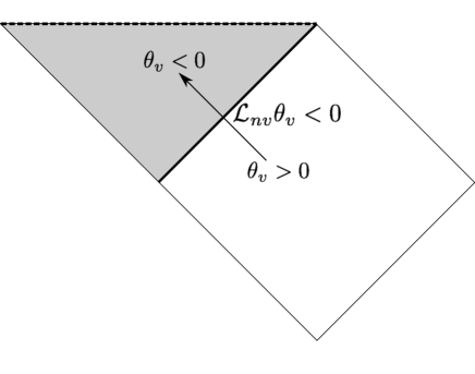
Figure 1: Penrose-Carter diagram for a Schwarzschild black hole. The dashed line represents the $R=0$ singularity and the heavy solid line represents a trapping horizon that is future ($\theta_{nv}=\theta_{-}<0$) and outer ($\mathcal{L}_{nv}\theta_{v}<0$, represented here by the null arrow).

Using this formalism within the Misner-Sharp-Hernandez approach, we can compute the expansion along the two future radial null directions. For the metric (2), the future outgoing radial null vector is

$$k^{a}=\left(\frac{1}{a},+\frac{1}{b},0,0\right)\ ,$$

and the future ingoing radial null vector is

$$l^{a}=\left(\frac{1}{a},-\frac{1}{b},0,0\right)\ ,$$

with normalisation $k^{a}l_{a}=-2$. We can then define the induced metric on the 2-spheres of symmetry, denoted by $h_{ab}$, as

$$h_{ab}=g_{ab}+\frac{1}{2}(k_{a}l_{b}+l_{a}k_{b})\ ,$$ (10)

and compute the expansions $\theta_{\pm}$ of outgoing and ingoing bundles of null-rays

$$\theta_{+} =h^{cd}\nabla_{c}k_{d}=\frac{2}{R}(U+\Gamma)\ ,$$ (11)

and

$$\theta_{-} =h^{cd}\nabla_{c}l_{d}=\frac{2}{R}(U-\Gamma)\ .$$ (12)

For a future trapping horizon (the black hole case), $\theta_{+}$ vanishes and $\Gamma=-U$ at the horizon, while for a past trapping horizon (in an expanding universe) $\theta_{-}=0$ and $\Gamma=+U$ at the horizon. In both cases

$$\theta_{+}\theta_{-}=\theta_{v}\theta_{nv}=\frac{4}{R^{2}}(U^{2}-\Gamma^{2})\ ,$$ (13)

with $\theta_{v}=0$ corresponding to $\Gamma^{2}=U^{2}$ and so, using Eq.(6), the result $R=2M$ (familiar for the event horizon of a Schwarzschild black hole) emerges as the condition for all spherically symmetric trapping horizons in spherically symmetric spacetimes. The general nature of this condition was already noted in the 1960s by Misner and his colleagues [25, 33] in the work which we are using as a basis for our present study.

An alternative way to arrive at this result is as follows. The general expression for changes in $R$ along a radial worldline

$$dR=\frac{\partial R}{\partial t}\,dt+\frac{\partial R}{\partial r}\,dr\,,$$ (14)

can be rewritten as

$$\frac{1}{a}\frac{dR}{dt}\!=\!\frac{dR}{d\tau}\!=\!\left(\frac{1}{a}\frac{\partial R}{\partial t}+\frac{1}{b}\frac{\partial R}{\partial r}\frac{b}{a}\frac{dr}{dt}\right)\!=\!\left(U+\Gamma v\right)\ ,$$ (15)

where

$$v\equiv\frac{b}{a}\frac{dr}{dt}\,,$$ (16)

is the 3-velocity of the object whose worldine is being considered, measured with respect to the local comoving frame of the fluid.

For radial null rays, inserting $ds=d\Omega=0$ into the metric (2) gives $a^{2}dt^{2}=b^{2}dr^{2}$, so that $v=\pm 1$, as expected, with the $+$ sign for an outgoing null ray and the $-$ sign for an ingoing one. Putting this into Eq.(15), and setting the right hand side to zero gives the condition for the trapping horizons as

$$\left.\frac{1}{a}\frac{dR}{dt}\right|_{\pm}=\left(U\pm\Gamma\right)=0\ ,$$ (17)

with $\Gamma=-U$ for future horizons and $\Gamma=+U$ for past horizons, as above, which again then both lead to $R=2M$.

Comparing Eq.(17) with Eqs.(11) and (12) gives

$$\theta_{\pm}=\frac{2}{R}(U\pm\Gamma)=\frac{2}{aR}\left.\frac{dR}{dt}\right|_{\pm}\ ,$$ (18)

which connects the geometrical approach involving the expansion $\theta$ used in [35] with the fluid approach used in [36]. Finally, note that the so-called apparent horizon of a black hole (a section of the future trapping horizon) is the outermost trapped surface for outgoing radial null rays while the trapping horizon for an expanding universe (which is a past trapping horizon) is foliated by the innermost past-trapped surfaces for ingoing radial null rays.

3 Causal Nature and Horizon Velocity

3.1 Causal Nature

Within the geometrical approach, the causal nature of the horizons mentioned above can be determined using the ratio of the Lie derivatives of the expansion that changes sign ($\theta_{v}$) in the two radial null directions [28]. This ratio, often denoted by $\alpha$, is defined as follows

$$\alpha\equiv\frac{\mathcal{L}_{v}\theta_{v}}{\mathcal{L}_{nv}\theta_{v}}\ ,$$ (19)

where evaluation at the horizon is implicit. The parameter $\alpha$ is negative/positive for timelike/spacelike horizons respectively, and goes to zero or infinity for null horizons. Now relating these Lie derivatives to the operators $D_{t}$ and $D_{r}$ of the Misner-Sharp-Hernandez formalism, we get

$$\mathcal{L}_{+}\theta_{v}=\mathcal{L}_{k^{a}}\theta_{v}=k^{a}\partial_{a}\theta_{v}\!=\!\left(\frac{1}{a}\frac{\partial}{\partial t}+\frac{1}{b}\frac{\partial}{\partial r}\right)\theta_{v}$$

$$\mathcal{L}_{-}\theta_{v}=\mathcal{L}_{l^{a}}\theta_{v}=l^{a}\partial_{a}\theta_{v}\!=\!\left(\frac{1}{a}\frac{\partial}{\partial t}-\frac{1}{b}\frac{\partial}{\partial r}\right)\theta_{v}$$

which gives

$$\mathcal{L}_{\pm}\theta_{v}=\left(D_{t}\pm D_{r}\right)\theta_{v}\ .$$ (20)

Then for the black hole case, where $\theta_{v}=\theta_{+}\propto(U+\Gamma)$ we have

$$\alpha=\frac{\mathcal{L}_{+}\theta_{+}}{\mathcal{L}_{-}\theta_{+}}=\frac{(D_{t}+D_{r})\theta_{+}}{(D_{t}-D_{r})\theta_{+}}=\left.\frac{(D_{t}U+D_{t}\Gamma)+(D_{r}U+D_{r}\Gamma)}{(D_{t}U+D_{t}\Gamma)-(D_{r}U+D_{r}\Gamma)}\right|_{H}\ ,$$ (21)

whereas in the case of an expanding universe, where $\theta_{v}=\theta_{-}\propto(U-\Gamma)$, we get

$$\alpha=\frac{\mathcal{L}_{-}\theta_{-}}{\mathcal{L}_{+}\theta_{-}}=\frac{(D_{t}-D_{r})\theta_{-}}{(D_{t}+D_{r})\theta_{-}}=\left.\frac{(D_{t}U-D_{t}\Gamma)-(D_{r}U-D_{r}\Gamma)}{(D_{t}U-D_{t}\Gamma)+(D_{r}U-D_{r}\Gamma)}\right|_{H}\ .$$ (22)

Using the Misner-Sharp-Hernandez equations, these two expressions for $\alpha$ turn out to give the same result, valid for both black holes and cosmology

$${\left.\alpha=\frac{4\pi R^{2}(e+p)}{1-4\pi R^{2}(e-p)}\right|_{H}}$$ (23)

where the $H$ indicates that the quantities are evaluated at the horizon location. (We note that this equation is equivalent to Eq.(2.7) of [37], with the quantity $C$ used in that work being equal to $2\alpha$ here.)

In A we briefly introduce the Misner-Sharp-Hernandez equations, guiding the reader through the algebra to derive Eq.(23).

3.2 Horizon Velocity

An alternative way of determining the nature and behaviour of the horizons is to calculate how they move with respect to the matter. This can be done by following the location where either of the defining conditions $\theta_{v}=0$ or $R=2M$ is satisfied. The two methods give the same result; for analogy with the derivation of $\alpha$, we choose also here to work with the expansion $\theta$. Maintaining $\theta_{v}=0$ along the worldline gives

$$d\theta_{v}=\frac{\partial\theta_{v}}{\partial t}\,dt+\frac{\partial\theta_{v}}{\partial r}\,dr=0\,,$$ (24)

leading to

$$D_{t}\theta_{v}+\frac{b}{a}\frac{dr}{dt}D_{r}\theta_{v}=0$$ (25)

at the horizon, so that its 3-velocity with respect to the matter, using the general definition of $v$ given by Eq.(16) evaluated here at the horizon location (cf. [37]), is then

$$v_{H}\equiv-\frac{D_{t}\theta_{v}}{D_{r}\theta_{v}}\ .$$ (26)

This expression is somewhat analogous to Eq.(19): in the hydrodynamical approach the proper time and proper space derivatives of the expansion $\theta_{v}$ are playing a similar role to that played in the geometrical approach by the Lie derivatives in the two null directions.

Differentiating through Eq.(13) and setting $\theta_{v}=0$, the expression for $v_{H}$ can be rewritten as

$$v_{H}=-\left.\frac{D_{t}\left(\Gamma^{2}-U^{2}\right)}{D_{r}\left(\Gamma^{2}-U^{2}\right)}\right|_{H}\ ,$$ (27)

or, by inserting into Eq.(26) the sum and difference of the two expressions in Eq.(20), it can be written as

$$v_{H}=-\left.\frac{\mathcal{L}_{+}\theta_{v}+\mathcal{L}_{-}\theta_{v}}{\mathcal{L}_{+}\theta_{v}-\mathcal{L}_{-}\theta_{v}}\right|_{H}\ ,$$ (28)

which leads to a direct relation between $\alpha$ and $v_{H}$

$$v_{H}=\pm\frac{1+\alpha}{1-\alpha}\ ,$$ (29)

with the plus for black hole formation and the minus for an expanding universe. Finally we can obtain an expression for $v_{H}$, analogous to Eq.(23) for $\alpha$, either by substituting that expression for $\alpha$ into Eq.(29) or by using Eq.(27) together with Eqs.(44) and (47) of A. This gives

$${v_{H}=-\left.\frac{U}{\Gamma}\right|_{H}\left.\frac{1+8\pi R^{2}p}{1-8\pi R^{2}e}\right|_{H}}$$ (30)

from which $v_{H}$ can be calculated in terms of quantities evaluated at the horizon location; $-\left.\frac{U}{\Gamma}\right|_{H}=\pm 1$ for future (black hole) and past (expanding universe) horizons respectively.

By definition, $v_{H}$ is positive for an outward-moving horizon and negative for an inward-moving one, with the “motion” here being measured with respect to the matter. In the following we refer to these respectively as outgoing and ingoing horizons, which does not always coincide with “outer” and “inner” horizons in the terminology of [4], as we will appreciate better in Section 4.

As mentioned earlier, because the horizon is a “mathematical” surface which does not correspond to any physical object, its velocity with respect to the fluid can be larger or smaller than the speed of light. More precisely, if $|v_{H}|>1$ (with $c=1$) the horizon is spacelike, if $|v_{H}|<1$ the horizon is timelike and if $|v_{H}|=1$ the horizon is null.

Evaluating Eq.(15) at the horizon location, with $v=v_{H}$, gives the evolution of the circumferential radius of the horizon $R_{H}$, which we will be discussing in Section 5. We note that this expression is nothing other than the Lie derivative of the circumferential radius $R$ taken along the vector field

$$t^{a}=\frac{1}{a}\left(1,-\frac{\partial_{t}(U\pm\Gamma)}{\partial_{r}(U\pm\Gamma)},0,0\right)\,,$$ (31)

which is tangent to the horizon (upper sign for black hole formation, lower sign for an expanding universe).

4 Black Hole Horizons

In this section, we implement the formalism and notation introduced in previous sections for studying the emergence and behaviour of trapping horizons during gravitational collapse to form black holes, focusing mainly on stellar collapse. While we will be using various simplifications, our eventual interest here is firmly focused on obtaining results having relevance for realistic astrophysical situations. We are considering here only “standard matter” for which $e$ is always positive and $p$ is non-negative, so that the null energy condition ($e+p\geq 0$) always holds.

We are restricting attention here to spherically symmetric non-rotating models. While this is certainly an important restriction (and we note the very interesting related work by Schnetter et al. [29] including rotation) the main features of interest for us are already present for non-rotating models. A number of the characteristic features seen in our present work confirm behaviour reported in [29]. The most important simplifications in our treatment are that we limit our matter model to representing an unmagnetized perfect fluid with a polytropic equation of state $p=K\rho^{\gamma}$, where $\rho$ is the rest-mass density and $K$ and $\gamma$ are constants (see B). Note that, while simplified, this does include pressure effects in a meaningful way if suitable values are taken for $K$ and $\gamma$. The case $K=0$ corresponds to idealised pressureless matter, often referred to as “dust”.

There have been important studies related to trapping horizons made in the context of pressureless matter. Some of this work has been extremely interesting (see, for example, [13] and [38]) but pressure effects play an important role in real stellar collapse to form black holes and can seriously change the picture as far as our present considerations are concerned. Viewing dust as a pressureless particle gas, the particles would strictly need to have zero velocity dispersion, corresponding to zero temperature, in violation of the third law of thermodynamics. Using dust as an approximation for collapse calculations can be relevant under certain circumstances but requires care since any initial non-zero velocity dispersion will tend to be amplified during collapse. While pressure gradients (the first term on the right hand side of Eq.(40) in A) become ineffective in the advanced stages of collapse due to falling values of $\Gamma$, the other effects of pressure typically become large then and should not be neglected.

Historically, some basic features of the behaviour of trapping horizons during collapse can already be seen in the paper by May & White [26], published fifty years ago, where they presented results from computations made with their version of the Misner-Sharp-Hernandez equations in A, going beyond the treatment given in the earlier classic paper by Oppenheimer & Snyder [39] by including non-zero pressure in the collapsing matter. We will start this section by briefly recalling the situation for the Oppenheimer-Snyder solution [39] for pressureless matter starting from constant density.

4.1 Oppenheimer-Snyder collapse

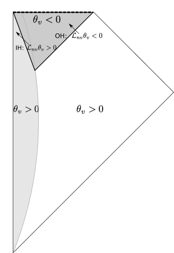
Figure 2: Oppenheimer-Snyder collapse. (Left) $2M/R$ plotted against $R/M_{*}$ (with $M_{*}$ being the total mass of the configuration) at successive levels of the coordinate time $t$, with the time increasing upwards. (Right) Penrose-Carter diagram for Oppenheimer-Snyder collapse: the collapsing ball of pressureless matter is represented in light grey, while the trapped region is shown in dark grey. The latter is bounded by solid lines representing the horizons, with IH indicating the inner horizon and OH indicating the outer one, according to the classification of [4] ($\mathcal{L}_{nv}\theta_{v}>0$ and $\mathcal{L}_{nv}\theta_{v}<0$ respectively, represented by the null arrows). Both OH and IH are here future horizons ($\theta_{nv}=\theta_{-}<0$). Note that in the special case of Oppenheimer-Snyder collapse, OH is also outgoing ($v_{H}>0$) and IH is ingoing ($v_{H}<0$).

In the Oppenheimer-Snyder solution, one has zero pressure and uniform energy-density on each time level, with the singular condition being reached simultaneously by all of the collapsing matter in terms of the cosmic time used in Eq.(2) which, for pressureless matter, is equivalent to the proper time of comoving observers. (From Eq.(43) it follows that if $p=0$ the lapse is constant and can be normalised to $1$).

For this, we have

$$M=\frac{4}{3}\pi R^{3}e\ ,$$ (32)

so that

$$\frac{2M}{R}=\frac{8}{3}\pi R^{2}e\ ,$$ (33)

from which it is clear that, since the energy density $e$ is a constant on each time slice, the condition $2M/R=1$ is first reached at the surface of the configuration, where the energy density drops discontinuously from its uniform interior value to zero. Figure 2 (left) shows the time evolution of the $2M/R$ curves, with the rising part of the curves corresponding to the matter configuration and the decreasing part to the vacuum outside. The horizons (occurring where $R=2M$, which is shown with the dashed line) are here formed first at the surface of the configuration (at the gradient discontinuity), and the subsequent locations of the ingoing horizon correspond to successive intersections of the $2M/R$ curves with the dashed line. One should think of the “outgoing” horizon as being formed in the vacuum outside the configuration, where it is immediately null with

$$v_{H}=1\ ,\quad\quad\quad\alpha=0\ ,$$ (34)

and it then remains at a constant value of $R$; the ingoing horizon is formed just inside the matter with $8\pi R^{2}e=3$ so that

$$v_{H}=-1/2\ ,\quad\ \alpha=-3\ ,$$ (35)

values which continue to apply through all of its subsequent evolution. The fact of the horizons being born as null and timelike in this case comes from the very special nature of the Oppenheimer-Snyder solution, for which the birthplace of the two horizons coincides with the density discontinuity going from the non-vacuum interior to the vacuum exterior. One can here interpret the ingoing and outgoing horizons as two separate surfaces appearing at the same location, already having different values of $\alpha$ and $v_{H}$, whereas for all of the other cases studied here, the horizons emerge from the separation into two parts of a single marginally trapped surface which at the moment of formation is neither ingoing nor outgoing.

Figure 2 (right) shows the Penrose-Carter diagram for this case, with IH and OH indicating the inner and outer horizons respectively. Note that, consistently with the behaviour in Figure 2 (left), IH and OH do not join to form a single smooth hypersurface in this case, there being a discontinuity in the tangent vector where they join, corresponding to the density discontinuity at the stellar surface.

4.2 Simulation I: the May & White case

In Figure 14 of the May & White paper [26], where $2M/R$ is plotted against their comoving rest-mass coordinate $\mu$ at a succession of times during the collapse, the peak local value of $2M/R$ can be seen rising to become equal to $1$ and then increasing further, leaving two locations where $2M/R=1$ which then separate, one going outwards with respect to the matter and the other going inwards (i.e. outgoing and ingoing horizons in the sense explained in the Introduction). The feature of the horizons forming in pairs has subsequently been discussed in various contexts by many other authors (including [29, 40, 41]). We decided that it would be interesting to repeat their calculations more or less exactly, but adding on the concepts which we have been presenting here regarding trapping horizons. In this sense, the following discussion can be seen as an addendum to their paper.

In a subsequent article, [42] they gave a very full account of how their computations were made, and we followed their methodology with only minor modifications (apart from needing to implement excision, so as to be able to follow the outgoing horizon all the way to the stellar surface). They used a standard type of largely explicit Lagrangian finite-difference method, with the comoving grid consisting of a succession of concentric spherical shells. The comoving radial coordinate of the outer boundary of each shell was identified with the time-independent value of the rest-mass $\mu$ contained within the sphere having this as its surface (i.e. $r$ was set equal to $\mu$, giving $b=1/4\pi R^{2}\rho$). They used 200 of these grid-zones, each containing the same amount of rest-mass $\Delta\mu$.

The 1966 paper deals both with stellar collapses which “bounce” and with continued collapse. We deal with just the latter here, for which they presented numerical results for collapse from rest of a $\gamma=5/3$, $21M_{\odot}$ polytropic sphere of matter having an initially uniform rest-mass density ($\rho_{0}=10^{7}{\rm g/cm^{3}}$) and specific internal energy ($\epsilon_{0}/c^{2}=9.61\times 10^{-7}$). (The $21M_{\odot}$ refers to the rest-mass of the configuration but, at this initial density, the rest-mass is essentially equal to the gravitational mass.) We successfully reproduced their results with these settings, but for the discussion below we needed a higher resolution and so used 2000 zones rather than 200. Also, we found that we could not get sufficiently clean results with their methodology if we started from a density as low as $10^{7}{\rm g/cm^{3}}$ and so we started instead from $10^{11}{\rm g/cm^{3}}$ but with the same value of $K$. This gave results with only surprisingly minor differences from theirs.

Figure 3: $2M/R$ is plotted against $\mu$ at successive levels of the coordinate time $t$, with the time increasing upwards. This is for a collapse starting from a constant-density initial model with $\gamma=5/3$. See text for further details.

The left hand frame of Figure 3 shows our plot of $2M/R$ versus $\mu$ corresponding to their Figure 14 but highlighting the points of interest to us here. The curves represent the solution at successive levels of the coordinate time $t$, with the time increasing upwards. (The total coordinate time for our run is two orders of magnitude smaller than May & White’s value, because of us starting from a higher density, but this is not relevant for our discussion.) Following the first (lowest) curve, representing the initial data, the next one up shows the moment when the curve first touches the condition $2M/R=1$ (marked by the dashed horizontal line). At later times, there are then two points of intersection of the respective curves with the horizontal line, marking the locations of the ingoing and outgoing horizons which then move apart as time progresses further (cf. Figure 1 of [43]). Note that these are locations with respect to the comoving coordinate $\mu$. The right hand frame shows an expanded view of the eventual approach of the ingoing horizon to the inner edge of the grid. When it reaches the outer edge of the innermost zone (the last point shown) it can no longer be tracked with the present version of the code; we will return to discussion of the behaviour close to $\mu=0$ at the end of this section.

These features are characteristic of collapses where the $R=2M$ condition is first reached within the bulk of the matter under conditions which are non-singular. Figure 4 shows a schematic representation of the growth of the trapped region: initially a single horizon forms (at $t=t_{1}$) which then separates into ingoing and outgoing horizons which move apart ($t=t_{2}$) until eventually the ingoing horizon approaches the centre of symmetry ($t=t_{3}$) while the outgoing horizon approaches the outer edge of the matter and goes on to become an event horizon when it reaches the vacuum outside. The fact that the initial trapped surface should separate into ingoing and outgoing parts, rather than into two parts going in the same direction (with respect to the matter, as discussed above) follows from the fact that, during collapse of classical matter ($p\geq 0$), the compactness $M/R$ calculated at constant values of $\mu$ is always increasing, as can be seen by calculating its time derivative:

$$D_{t}\left(\frac{M}{R}\right)=-\frac{U}{R}\left(\frac{M}{R}+4\pi R^{2}p\right)\,,$$ (36)

where Eq.(47) has been used. This is always positive when the matter is collapsing ($U<0$) and so the two locations where $R=2M$, arising after the separation, must then move in opposite directions (cf. Figure 3).

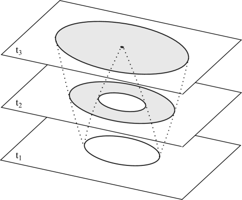
Figure 4: Schematic representation of the time-foliation of our spacetime. The non-shaded parts of the drawing are the untrapped regions ($\theta_{+}>0$), the shaded parts are the trapped regions ($\theta_{+}<0$), and the solid lines are the horizons ($\theta_{+}=0$). At first a single trapped surface appears, which then separates into an outgoing horizon and an ingoing horizon. Their evolution in terms of the radial coordinate $r=\mu$ is shown by the dotted lines.

In the left frame of Figure 5, we have plotted the energy density $e$ as $e/c^{2}$ (in units of ${\rm g/cm^{3}}$) against $\mu$, for the same case as in Figure 3. Here the horizontal dashed line marks the initial data, the next curve up is for the time at which the condition $2M/R=1$ is first reached, and the successive curves are then for subsequent times (time increasing upwards). (May & White plotted instead the rest mass density $\rho$, but it is the energy density which will concern us here.) The dots show locations of the ingoing horizon and will enter into our discussion below (the locations of the outgoing horizon are not shown here because they get confused among the closely-packed curves in the outer region). Initially there is a step discontinuity of the density (and pressure) at the surface of the configuration and this subsequently decays, giving a pressure gradient which works its way inwards. For a region where the pressure gradient remains zero, the density remains uniform (in this slicing), i.e. $e=e(t)$ with no dependence on $\mu$. Eventually (after the time of the third solid curve) the uniform region disappears completely and a density cusp appears at $\mu=0$. Finally, an off-centred density maximum appears which goes on to form the curvature singularity, as was widely discussed in the 1960s (see [33], for example). The right-hand frame of Figure 5 shows a similar plot for $R$ (in units of km) versus $\mu$ (here time is increasing downwards). Note that at the curvature singularity, $R=0$ (as expected) but $\mu\neq 0$ and, indeed, comprises a considerable fraction of the total rest mass. However, one needs to be cautious about this because the picture depends on the slicing used and while $\mu$ is defined in a clear physical way, the time coordinate $t$ is not, and depends on an arbitrary slicing choice. We are seeing here curves drawn at a succession of constant values of this coordinate $t$.

Figure 5: Plots of $e/c^{2}$ (in units of ${\rm g/cm^{3}}$) and $R$ (in units of km) against $\mu$ at successive levels of the coordinate time $t$, for the same case as in Figure 3, with the time increasing upwards in the left-hand panel and downwards in the right-hand one. See text for further details.

At this point, it is relevant to make some general comments (and we apologize to readers for whom this is well-known and obvious). General relativity is fully four-dimensional and reality resides in the full four-dimensional spacetime. It is a matter of convenience for us, in making calculations, to split the spacetime into 3 dimensions of space plus 1 of time. How this slicing is made is a matter of choice, and which events appear as simultaneous depends on this choice. Also, whether particular events in the four-dimensional spacetime appear or not with the slicing being used, depends on whether it reaches far enough to “see” them. Because an event in the 4D spacetime is not “seen” by a given slicing does not mean that it does not exist. It is fundamental to the idea of a trapping horizon that it is a spacetime concept, defined quasi-locally, which does not depend on the asymptotic behaviour of a Cauchy slice [20, 21]. Of the quantities which we are using here in our discussion, $R$ is invariantly defined (either as proper circumference divided by $2\pi$ or as an areal radius), $\mu$ is a physically-defined quantity, $b\,d\mu$ and $a\,dt$ are intervals of radial proper distance and proper time, as measured by observers comoving with the fluid, $v_{H}$ and $\alpha$ are defined directly in terms of $b\,d\mu$ and $a\,dt$, and $e$ and $p$ are measured in the fluid rest frame. It is true that working in the local comoving frame represents a choice, but comoving observers form a privileged class (see also [14]).

Figure 6: Plots of $|v_{H}|-1$ (solid curves) and $1/\alpha$ (dot-dashed curves) as functions of $\mu$; this is for the standard $\gamma=5/3$ case for collapse from rest of a $21M_{\odot}$ model with constant-density initial conditions. The right-hand frame shows an enlargement of the behaviour at small $\mu$. The arrows in the left-hand frame show the directions of time increasing along the horizon curves, the circle and vertical dashed line mark where the horizons form.

Bearing in mind that Figures 3 and 5 need to be treated with some caution, we now proceed to discuss the behaviour of the trapping horizons using the quantities listed above. It is, of course, important to use a slicing for our numerical calculations in which the events which we want to study can be “seen”, but the diagonal slicing used by May & White does satisfy that. Figure 6 shows the behaviour of the locally-measured horizon three-velocity $v_{H}$ and the parameter $\alpha$ for the outgoing and ingoing horizons from our standard run as described above (the right-hand frame shows an enlargement of the behaviour at small $\mu$). We have plotted the quantities $|v_{H}|-1$ (solid curves) and $1/\alpha$ (dot-dashed curves); each of these is greater than zero if the horizon is spacelike, equal to zero if it is null, and less than zero if it is timelike. The behaviour seen can be summarized as follows. The horizons are born as a pair by the separation into two parts of the initial single marginally trapped surface formed when the $2M/R$ curve becomes tangent to $1$, as seen in Figure 3. They begin to separate with infinite velocity, one going outwards with respect to the matter and the other going inwards. At the birth ($|v_{H}|\to\infty$), $\alpha=1$; this can be understood from the fact that the first contact between the slicing and the 3-horizon is tangential. It then follows from Eq.(30) that $8\pi R^{2}e=1$ at the point of birth, i.e. $e=1/2A_{H}$ there, where $A_{H}$ is the area of the horizon - an intriguing result. Both horizons then slow down as they move, the outgoing horizon becoming asymptotically null as it approaches the surface of the configuration and becoming a static event horizon when it reaches the vacuum. (Note that $v_{H}$ is always measured with respect to the local infalling matter; the event horizon is outgoing and null with respect to local light cones but is static in that it remains at a constant value of $R$.) Meanwhile, $1/\alpha\to\infty$, so that $\alpha\to 0$ at the surface, as expected. As the ingoing horizon slows down, it becomes timelike for a while before becoming spacelike again and eventually going back to the conditions ($|v_{H}|\to\infty$, $\alpha=1$) which it had at birth. Comparing this with Figure 5, note that the pair of horizons first forms at a value of $\mu$ outward of that for the singularity and that the uniform-density region is reached by the ingoing horizon while it is timelike. The rise of $|v_{H}|$ back towards infinity happens when the ingoing horizon encounters the rising part of the profile for $e$, leading towards the cusp at $\mu=0$. All of the latter parts of this happen at values of $\mu$ smaller than that at which the singularity forms. As mentioned in connection with Figure 3, we are not able to follow evolution of the ingoing horizon extremely close to $\mu=0$ with our current methodology due to the finite resolution of the code: the last point shown for it in the figures is where it reaches the outer edge of our innermost zone, and $|v_{H}|$ has not yet diverged to infinity there ($\alpha$ is extremely close to $1$ but not coincident with it). It seems clear that the behaviour seen must be modified very close to $\mu=0$ and we suspect that the ingoing horizon is stopped before reaching there, as we will discuss further in Section 4.4.

The behaviour seen in this simulation is rather different from that for the Oppenheimer-Snyder collapse described in the previous subsection, where the ingoing and outgoing horizons first appear already as separate entities. Another special feature of the Oppenheimer-Snyder solution is the one-to-one correspondence between outgoing/ingoing horizons and outer/inner horizons in the Hayward terminology, which does not arise for our simulations with non-zero pressure. Also, the combination of homogeneity and zero pressure preserves the density discontinuity at the surface which non-zero pressure instead removes due to the action of pressure gradients during the collapse. Note, however, that if one makes a dust calculation for models with non-uniform initial density profiles having no density discontinuity at the surface, such as the Lemaître-Tolman-Bondi (LTB) models discussed in [13] (we have repeated those calculations), one again observes some cases where the horizons first emerge from a single trapped surface formed within the matter, which then separates into ingoing and outgoing horizons with a smooth join between them, reproducing the standard behaviour observed in Figure 3. In those cases, the horizons again start with $\alpha=1$ and $|v_{H}|\to\infty$ but if the inner part of the initial density profile is nearly constant, one observes the Oppenheimer-Snyder values of $\alpha$ and $v_{H}$ being reached asymptotically as limiting values with no eventual return to the conditions at birth.

Figure 7: Equivalent plots to those in Figure 6, but this time with $\gamma=4/3$ rather than $5/3$. The solid curves again show $|v_{H}|-1$ while the dot-dashed curves show $1/\alpha$. The directions of time increasing along the horizon curves are the same as in Figure 6 with the circle marking the location of horizon formation while the arrows show the directions of time increasing along the horizon curves.

4.3 Simulations II & III: further polytropic models

We wanted to investigate how the situation shown in Figure 6 would change when the polytropic model for the configuration was altered. May & White had chosen to use a model with a rest mass of $21M_{\odot}$ with a $\gamma=5/3$ polytropic equation of state (representing a non-relativistic monatomic particle gas). For our first alternative model, we replaced $\gamma=5/3$ by $\gamma=4/3$, but kept everything else the same, including the initial value of $p/\rho$ (checking that this still ensured continuing collapse rather than a collapse and bounce). We chose $\gamma=4/3$ (corresponding to a relativistic particle gas) because in the limit where the internal energy becomes very much larger than the rest-mass energy, this tends towards a $p=we$ equation of state with $w=1/3$, as used for cosmological calculations in the radiative era of the early universe. The internal energy becomes progressively larger with respect to the rest-mass energy as the collapse proceeds but, in our calculation, it never quite reached the asymptotic regime. Our results are shown in Figure 7. The initial and final conditions for the horizons are similar to before; the most important difference seen is the long horizontal part of the curves for $|v_{H}|-1$ and $1/\alpha$ when the ingoing horizon is timelike. The reason for this can be understood by looking again at Figure 5 (for $\gamma=5/3$). The horizontal regions of uniform energy density are longer in the $\gamma=4/3$ case, so that the ingoing horizon is traversing spatially uniform matter for longer, meaning that there is a substantial part of the evolution which is similar to the Oppenheimer-Snyder solution ($p/e$ is quite small there). In contrast, for the $\gamma=5/3$ case the ingoing horizon only reached the uniform density region just before that disappeared.

Figure 8: Equivalent plots to those in Figure 6, using a $\gamma=5/3$ equation of state but starting from a $21M_{\odot}$ model in hydrostatic equilibrium, which was then destabilized by decreasing $K$. The solid curves again show $|v_{H}|-1$ while the dot-dashed curves show $1/\alpha$. The directions of time increasing along the horizon curves are the same as before with the circle marking the location of horizon formation while the arrows show the directions of time increasing along the horizon curves.

The next trial returned to $\gamma=5/3$ but abandoned constant density for the initial model, using instead a model in hydrostatic equilibrium, near to the radial instability limit, which was then made unstable to collapse by decreasing $K$. We again retained $21M_{\odot}$ as the mass, for uniformity with the May & White value. Results are shown in Figure 8.

Here, the pair of horizons are born at a much smaller value of $\mu$, because of the density being much higher in the central regions than further out, and there is never any uniform density region. In this case, the ingoing horizon is always spacelike (the reverse situation to the Oppenheimer-Snyder case). The other main features have been seen in all of the polytropic simulations which we have investigated here (horizons born as a pair, separating initially with infinite velocity and then slowing down; outgoing horizon being always spacelike but becoming asymptotically null as it reaches the stellar surface; ingoing horizon always being spacelike at the end and tending to infinite velocity close to $\mu=0$).

Figure 9 shows $8\pi R^{2}e$ (evaluated at the horizon location) plotted as a function of $\mu$ for each of the polytropic simulations. This is the key quantity appearing in the denominator of Eq.(30). The circles mark the join between the results for the ingoing and outgoing horizons, at the point where they form (with $8\pi R^{2}e=1$ as mentioned earlier). Note the long horizontal section at the Oppenheimer-Snyder value of $8\pi R^{2}e=3$ for the $\gamma=4/3$ case starting from constant density, while this value is only barely reached for the corresponding $\gamma=5/3$ case. For the run starting from hydrostatic equilibrium, $8\pi R^{2}e$ at the horizon peaks at a value less than $3$. In the two runs starting with a homogeneous profile, the horizon is forming closer to the surface of the star and the ingoing horizon is able to become timelike, eventually reaching the homogeneous condition $8\pi R^{2}e=3$, whereas in the run starting from hydrostatic equilibrium the horizon forms much closer to the centre and the ingoing horizon remains always spacelike. In all of the cases, there is eventually a rapid fall towards $1$ as the horizon enters the region of increasing density leading up to the cusp.

Figure 9: The quantity $8\pi R_{H}^{2}e_{H}$ is plotted against $\mu$ for each of the three cases studied. HOM indicates cases where the initial model was homogeneous (i.e. had constant density); TOV indicates that the initial model was obtained by solving the TOV equations of hydrostatic equilibrium and then making it unstable to collapse by reducing $K$. The circles indicate the join between ingoing and outgoing horizons.

4.4 LTB models and the final state of the ingoing horizon

If $|v_{H}|\to\infty$ (with $\alpha=1$ and $e_{H}=1/2A_{H}$) is genuinely the “final” condition for the ingoing horizon, as seems to be indicated by each of our three simulations, the fact that $e_{H}$ is not diverging there (see Figure 5) indicates that $A_{H}$ should also be finite at the end and, if so, the ingoing horizon must be stopped before reaching $\mu=0$ (unless $A_{H}$ could somehow be non-zero there). Our simulations, made following the methodology of May & White [26], are limited in seeing very small-scale phenomena by the use of a finite-spaced grid, but we thought it useful to look for hints about the possible eventual behaviour of the ingoing horizon from the quasi-analytic LTB dust models. As mentioned previously, the very interesting LTB calculations with smooth non-uniform density profiles presented in [13] include cases where the initial behaviour is rather similar to that seen in our simulations, and there is one case where the ingoing horizon is indeed beingstopped before reaching the centre (although this is not commented on in their paper). In Figure 10, we show results from our re-calculation of this case in terms of the quantities which we are using in this paper, apart from following the previous authors’ use as a comoving coordinate of the circumferential (areal) radius of each shell at the initial time, which they denote by $r$. The model concerned is the $\sigma=2$ model from Section 3.3.2 of their paper, and we refer the reader to [13] for further details of this and other associated models. Note that the use of $r$ as a radial coordinate effectively expands the innermost regions and contracts the outer ones with respect to what one would see using our mass coordinate $\mu$.

Figure 10: The left-hand frame shows $2M/R$ plotted against $r$, at successive values of the comoving proper time, for the LTB model of [13] with $\sigma=2$. The right-hand frame shows the corresponding behaviour for $\alpha$ and $v_{H}$ with the solid curves representing $|v_{H}|-1$ and the dot-dashed curves representing $1/\alpha$. The directions of time increasing along the horizon curves are the same as in Figure 8 with the addition of a secondary outgoing horizon forming at $r=0$ which moves outward along the $\alpha$ and $v_{H}$ curves until it meets and annihilates with the ingoing horizon at the inner location where $v_{H}$ diverges.

In the left-hand frame, we have plotted the behaviour of $2M/R$ at successive levels of the comoving proper time (with time increasing upwards). The lowest curve is for the initial time, the next one up is at the time when $2M/R$ first becomes equal to $1$ and then the following curves are at equal time intervals around the time when the ingoing horizon is stopped. The ingoing and outgoing horizons (located at the points where $2M/R=1$) initially form together inside the matter and then separate, as seen in the simulations, but the ingoing horizon eventually meets a secondary outgoing one emerging from $r=0$, where a singularity has formed, and annihilates with it, leaving only the outer outgoing horizon. The right-hand frame shows the corresponding behaviour of $|v_{H}|$ and $\alpha$, with the arrows marking the direction of motion along the $|v_{H}|$ curves. The two main horizons form as a pair at $r\simeq 2$ where $|v_{H}|$ diverges and $\alpha=1$ (marked with an open circle). They then separate as usual, both being spacelike. The velocity $|v_{H}|$ of the ingoing horizon first decreases but reaches a minimum velocity (still spacelike) and then increases again towards the left-hand divergence at $r\simeq 0.33$. There it approaches the inner outgoing horizon and annihilates with it at the point where $\alpha$ is again equal to $1$ (filled circle). The processes of formation and annihilation appear as identical here, only with opposite directions of the arrow of time.

It can be seen that this reproduces some of the key points of the phenomenology seen in the simulations: the horizons forming together with $|v_{H}|\to\infty$ and $\alpha=1$ and then separating, followed by the ingoing horizon ending again with the same conditions. However, other aspects (including the nature of the singularity formation) are significantly different because of pressure effects and associated changes in the time slicing. It remains to be seen the extent to which the process described above for the stopping of the ingoing horizon, corresponds to what occurs in physical cases where there is non-zero pressure.

5 Causal Nature: a general perspective

Here we give a more general overview of the types of behaviour which we have observed in the numerical simulation results, summarising the different phenomenologies within a coherent picture. We stress that everything in this section refers to strictly spherically symmetric horizons within a spherically symmetric spacetime. First we recall that for black hole trapping horizons, it is the outward expansion $\theta_{+}$ which vanishes, these being future horizons in the Hayward terminology, with $\Gamma=-U$ at the horizon location. As we show in the following, it is useful to exhibit the simulation results on a plot of $v_{H}$ against $\alpha$, since this allows identification of all of the conceivable horizon behaviours within the scenario being considered here, together with indicating the corresponding conditions for energy density and pressure. Using Eq.(29) written for the black hole case, we have

$$v_{H}=\frac{1+\alpha}{1-\alpha}\,,$$ (37)

which is represented by a rectangular hyperbola, as shown in Figure 11. This expression is very general, based only on the definitions of these quantities in spherical symmetry (see Section 3), and does not depend on the particular form of the equation of state or of the stress energy tensor. It links together the geometrical approach to the causal nature, represented by $\alpha$, and the hydrodynamical one, represented by $v_{H}$, corresponding to the two sides of the Einstein equation. Although $\alpha$ and $v_{H}$ are not independent quantities, we suggest that discussing both of them together is useful for clarifying the physical meaning of some key features, creating a common ground of understanding between the geometrical and hydrodynamical approaches.

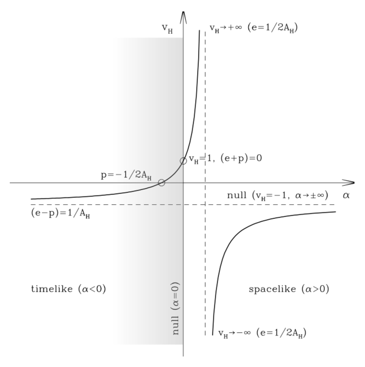
Figure 11: Plot of $v_{H}$ versus $\alpha$ for the black hole horizons. The significance of the points indicated in the figure is described in the text.

For collapse of a perfect fluid $\alpha$ and $v_{H}$ are given by

$$\alpha=\frac{4\pi R_{H}^{2}(e+p)}{1-4\pi R_{H}^{2}(e-p)}\ ,\phantom{spacing}v_{H}=\frac{1+8\pi R_{H}^{2}p}{1-8\pi R_{H}^{2}e}\ ,$$ (38)

(in this sub-section, $e$ and $p$ will always be evaluated at the horizon location and so we omit the subscript $H$ for them). For normal matter, not violating the null energy condition (NEC) $e+p\geq 0$, the numerator of the expression for $\alpha$ is always positive and the sign of $\alpha$ (determining the signature of the horizon) is the same as that of the denominator (proportional to $-{\mathcal{L}_{-}\theta_{+}}$). The behaviour of this depends on the initial density profile of the configuration and on the equation of state, as we have seen from the simulation results presented here.

As we have already mentioned when discussing Figure 3: for collapses where the $R=2M$ condition is first reached within bulk of the matter, under conditions which are non-singular, a single marginally trapped surface appears there with $\alpha=1$ and with the local value of the energy density being $e=1/2A_{H}$, independently of the pressure. As can be seen from Figure 11, this is the only location in the diagram where a horizon with $e$ and $p$ non negative is neither ingoing or outgoing. The initial marginally trapped surface then separates into a pair of horizons, one outgoing and one ingoing, with $v_{H}\to\pm\infty$. The outgoing horizon, which is always spacelike, starts at the top of the upper branch of the hyperbola and then rolls down it, eventually reaching the stationary state corresponding to a null isolated horizon with $v_{H}=1$ when all of the collapsing matter has passed through it, so that $(e+p)=0$ at the horizon location. The ingoing horizon is also initially spacelike but starts at the bottom of the lower branch of the hyperbola, and then rolls up it, possibly passing to the upper branch (the two branches are connected via $\alpha\rightarrow\pm\infty$) where it comes in from the left as a timelike horizon and continues to roll upwards.

The change from spacelike to timelike corresponds to satisfying the condition $e-p=1/A_{H}$, for which the denominator of the left hand relation in Eq.(38) vanishes. Once again, we observe here a connection between fluid quantities (energy density and pressure) and a geometrical one (horizon area). Whether or not the change to timelike occurs seems to depend on the initial density profile of the configuration and on the equation of state. We have observed it happening for the constant-density initial models (with both $\gamma=4/3$ and $\gamma=5/3$) but not for the model starting from hydrostatic equilibrium, where the ingoing horizon always remained spacelike.

In each of our three cases, whether the ingoing horizon passes to the upper branch or not, it eventually reaches a maximum height on the plot and then rolls down the hyperbola again, ending on the lower branch, going back to $v_{H}\to-\infty$ and $\alpha=1$ from where it started. This is different from what happens with the the constant-density, zero-pressure Oppenheimer-Snyder collapse model, where the behaviour is characterised by constant values of $\alpha$ and $v_{H}$. However, as discussed above, that is a limiting case of the set of pressureless LTB models studied in [13] which have no density discontinuity at the surface and for many of which the horizon formation follows the standard picture described above (with $\alpha=1$), even if other aspects of the evolution are significantly different from the situation with non-zero pressure. In one of the LTB models ($\sigma=2$) where the Oppenheimer-Snyder limit is not approached in the centre, we see a second outgoing horizon emerging from the singularity formed at $r=0$ with $v_{H}\simeq 1$, rolling along the upper branch of the hyperbola up to $v_{H}\to+\infty$ where it meets and annihilates with the ingoing horizon which is rolling along the lower branch down to $v_{H}\to-\infty$. This is consistent with what we have seen in our runs near $\mu=0$, and shows the identical geometrical nature of the formation/annihilation processes for ingoing and outgoing horizons.

We now give a coordinate-independent interpretation of the increase (or decrease) of the horizon area using Eq.(15), which gives

$$\mathcal{L}_{t^{a}}R_{H}=\left.\frac{dR}{d\tau}\right|_{H}=U_{H}(1-v_{H})\ ,$$ (39)

with $U$ always being negative because the matter is collapsing. Thus the area $A_{H}$ increases along the path of the horizon if $v_{H}>1$, and decreases if $v_{H}<1$. For a classical fluid, energy and pressure are both positive and the NEC is not violated. Under these circumstances the outgoing horizon is spacelike, (null just in the limit, as in the vacuum Schwarzschild solution) and $A_{H}$ is always increasing, while in general $A_{H}$ is always decreasing for an ingoing horizon. If the NEC is violated, with the pressure becoming negative, the outgoing horizon is allowed to roll down the upper branch of the hyperbola beyond $v_{H}=1$, becoming timelike with a decreasing $A_{H}$, signifying a shrinking surface. This happens in the presence of Hawking radiation, consistently with the fact that a timelike outgoing horizon ($0<v_{H}<1$), allows emission to go through the horizon [44, 45]. Note also the consistency of the horizon still being outgoing in the presence of Hawking radiation, remembering that $v_{H}$ is measured with respect to the collapsing matter.

In our simulations, we considered only classical matter with $e$ and $p$ positive which excludes one conceivable horizon configuration, i.e. the inner and outgoing horizon. Indeed, the latter simultaneously has $\mathcal{L}_{-}\theta_{+}\propto[(e-p)-1/A_{H}]>0$ because it is inner, and $v_{H}>0$ because it is outgoing, and therefore from Eq.(38) we must have $p<-1/2A_{H}<0$. Hence for a classical fluid the outgoing horizon can only be outer. Whenever the NEC is satisfied (as it is for a classical fluid) there is a strict one-to-one correspondence between spacelike and outer on the one hand, and timelike and inner on the other hand (see theorem 2 of [4], and [13]). Since the outgoing horizon can only be outer for classical matter, it must therefore be spacelike whereas the ingoing horizon can sometimes be spacelike (outer) and sometimes timelike (inner). Having this classically excluded configuration (inner and outgoing) seems to confirm the possibility of using the relation between $\alpha$ and $v_{H}$ also within the context of quantum effects (such as Hawking evaporation, mentioned before) which indeed allow having negative pressure and/or violation of the energy conditions.

The intersection with the horizontal axis is another special point of the hyperbola with $\alpha=-1$ and $v_{H}=0$, corresponding to the geometrical relation $p=-1/2A_{H}$, which for a homogeneous and isotropic fluid corresponds to $(e+3p)=0$. In this case the value of $A_{H}$ is independent of the energy density and depends only on the pressure, a symmetric relation to the one at the point of horizon formation ($\alpha=1$ and $v_{H}=\pm\infty$, with $e=1/2A_{H}$ independently of the value of the pressure). This point of the hyperbola represents the situation for a horizon which is neither outgoing nor ingoing, but is instead comoving with the collapsing matter. Rolling down the hyperbola, an outgoing horizon passing through this point would then become ingoing, while an ingoing horizon rolling up along the hyperbola would instead become outgoing. This corresponds to a turnaround of the horizon with respect to the matter. The location of the transition point for the ingoing horizon where it goes from positive values of the pressure to negative ones, depends on the particular value of the energy density. If this value is always smaller than or equal to the value for the homogeneous regime ($e=3/8\pi R^{2}$), as seen in Figure 9 for our simulations, the pressure will become negative for values of $v_{H}$ limited by the Oppenheimer-Snyder value (i.e. $v_{H}\leq-1/2$). Instead, if the energy density is reaching values larger than the homogeneous regime, then the pressure will change sign between the Oppenheimer-Snyder value and the point where the horizon is comoving with the matter (i.e $-1/2<v_{H}<0$). In Figure 11 the region of possible negative pressure has been highlighted in grey, degrading where the change of sign would occur.

If an ingoing horizon becomes outgoing with a turnaround and keeps rolling up to $v_{H}=1$ and $\alpha=0$, then from Eq.(39) $A_{H}$ will start increasing, signifying that the horizon bounces. Such a bounce has been proposed as an alternative to the classical result of black hole singularity formation [46, 47, 48, 49]. Although these scenarios are quite speculative, and we are not trying to draw any conclusion regarding them here, we think that it is worth pointing out that they could in principle be included within this sort of discussion of $\alpha$ and $v_{H}$. In future, we plan to investigate some of these possibilities using an equation of state including quantum phenomenology which allows for violation of the energy conditions.

6 Summary and Conclusions

In the present paper, we have brought together the Misner-Sharp-Hernandez hydrodynamical formalism for calculations in spherical symmetry and the geometrical formalism normally used for discussing trapping horizons. We have given our motivations and explained why quasi-local horizons are useful in dynamical situations such as collapse to form black holes. By relating the expansion of the null geodesic congruence $\theta$ to the hydrodynamical parameters $U$ and $\Gamma$, we have confirmed that the horizons which appear in the Misner-Sharp-Hernandez formalism are precisely trapping horizons (we have used this term for 3D hypersurfaces as well as 2D surfaces here) and can be defined equivalently as loci where $U\pm\Gamma$ vanishes or where $\theta_{\pm}=0$, both corresponding to $R=2M$.

We then used this unified framework to study trapping horizons, focusing on the geometrical $\alpha$ (the sign of which gives the causal nature of the horizon), and the hydrodynamical $v_{H}$, which is the three velocity of the horizon with respect to the collapsing/expanding fluid. For a perfect fluid medium, each can be expressed as a simple algebraic function of the energy density and pressure of the fluid at the location of the horizon, and they can also be expressed as simple functions of each other.

We applied this formalism and notation to the study of black hole formation, presenting results from numerical simulations of spherically symmetric stellar collapse similar to those made in 1966 by May & White [26] but focusing now on the behaviour of the trapping horizons. Following the line of the previous work, we investigated three sample cases, all including pressure effects using a polytropic equation of state. Two started from constant density but with different values of the adiabatic index $\gamma$ ($5/3$ and $4/3$), while the third, more realistic, case started from a configuration in hydrostatic equilibrium which was then made unstable to collapse by reducing the parameter $K$. We note that, in many respects, our results are rather different from those given by the analytic Oppenheimer-Snyder solution [39] for pressureless collapse from constant-density initial conditions. More elaborate studies of pressureless collapse, using LTB models with non-uniform density [13] show greater similarity with the present work but there are still significant differences and, in general, one should treat with caution the use of calculations with pressureless matter as a guide for realistic physical situations in the present context.

Our simulations all show the formation of a marginally trapped surface within the collapsing matter with $\alpha=1$ which then separates into two parts, one moving outwards ($v_{H}>0$) and the other moving inwards ($v_{H}<0$) with respect to the matter. Both of these horizons form spacelike with $v_{H}\to\pm\infty$. For any classical fluid not violating the NEC, it is known that the outgoing horizon (which is an outer horizon according to Hayward’s terminology) must remain spacelike while passing through the collapsing matter and this is indeed seen in the simulations with the horizon eventually becoming null when all of the collapsing matter has passed through it. At the final stage, it is an isolated horizon in vacuum, equivalent to the event horizon of the Schwarzschild solution. For the two cases starting from constant density, the ingoing horizon starts spacelike, subsequently becomes timelike, and then goes back to being spacelike again at the end; for the case starting from hydrostatic equilibrium, it always remains spacelike. In all cases, the ingoing horizon continues to move towards $\mu=0$, finally shrinking away there with $\alpha\to 1$ and $v_{H}\to-\infty$, the same conditions as when it was formed. Plotting the functional relationship between $\alpha$ and $v_{H}$ gives a rectangular hyperbola, and we found that this gives a convenient way of exhibiting the horizon evolution, leading to additional insights. The roles of differing initial configurations and differing equations of state require further investigation with a more systematic analysis, and we are now embarking on that.

Appendix A Misner-Sharp-Hernandez equations

Here we present the Misner-Sharp-Hernandez equations in the composite form based on [24, 25, 26] which we have used for the work reported in this paper. Consider the “cosmic time” metric given by Eq.(2) with the definitions of $U$, $\Gamma$ and $M$ given in Eqs.(4), (5), (9) and a perfect fluid with stress energy tensor $T^{a}_{\phantom{a}b}=\textrm{diag}(-e,p,p,p)$ (consistent with Eq.(7)), where $e$ is the energy density and $p$ is the pressure. Then the Misner-Sharp-Hernandez hydrodynamic equations obtained from the Einstein equations and the conservation of the stress energy tensor are:

$$D_{t}U=-\frac{\Gamma}{e+p}D_{r}p-\frac{M}{R^{2}}-4\pi Rp\,,$$ (40)

$$D_{t}\rho=-\frac{\rho}{\Gamma R^{2}}D_{r}(R^{2}U)\,,$$ (41)

$$D_{t}e=\frac{e+p}{\rho}D_{t}\rho\,,$$ (42)

$$D_{r}a=-\frac{a}{e+p}D_{r}p\,,$$ (43)

$$D_{r}M=4\pi R^{2}\Gamma e\,,$$ (44)

where $\rho$ in Eqs.(41) and (42) is the rest mass density (or the compression factor for a fluid of particles without rest mass). These form the basic set, together with the constraint equation given already by Eq.(6),

$$\Gamma^{2}=1+U^{2}-\frac{2M}{R}\,.$$ (45)

Two other useful expressions coming from the Einstein equations are

$$D_{t}\Gamma=-\frac{U}{e+p}D_{r}p\,,$$ (46)

$$D_{t}M=-4\pi R^{2}Up\,.$$ (47)

In order to derive the expression for $\alpha$ given by Eq.(23) we need to make some manipulation of these equations. Combining Eqs.(40) and (46) gives

$$D_{t}U\pm D_{t}\Gamma=-\frac{\Gamma\pm U}{e+p}D_{r}p-\frac{M}{R^{2}}-4\pi Rp\,.$$ (48)

Differentiating $\Gamma$ with respect to $r$ in Eq.(45) gives

$$D_{r}\Gamma=\frac{U}{\Gamma}D_{r}U+\frac{M}{R^{2}}-\frac{1}{\Gamma R}D_{r}M\,,$$ (49)

that combined with Eq.(44) allows one to write

$$D_{r}U\pm D_{r}\Gamma=\frac{\Gamma\pm U}{\Gamma}D_{r}U\pm\frac{M}{R^{2}}\mp 4\pi Re\,.$$ (50)

Using now expressions (48) and (50) appearing in Eqs.(21) and (22) with the corresponding conditions for the black hole horizons ($\Gamma=-U$) and for the cosmological horizon in an expanding universe ($\Gamma=U$), we obtain

$$\alpha=\left.\frac{4\pi R^{2}(e+p)}{1-4\pi R^{2}(e-p)}\right|_{H}$$ (51)

in both cases, which is Eq.(23).

Appendix B Equation of state

In order to solve the set of equations presented in the previous Appendix we need to supply an equation of state specifying the relation between the pressure and the different components of the energy density. For a simple ideal particle gas, we have that

$$p=(\gamma-1)\rho\epsilon\,,$$ (52)

where $\epsilon$ is the specific internal energy, related to the velocity dispersion (temperature) of the fluid particles and $\gamma$ is the adiabatic index. The total energy density $e$ is the sum of the rest mass density and the internal energy density:

$$e=\rho(1+\epsilon)\,.$$ (53)

Putting these equations into the energy equation (42), one gets the standard polytropic form used for stellar models

$$p=K\rho^{\gamma}\,,$$ (54)

where $K$ is a constant of integration (varying with the specific entropy if the process is not adiabatic), and $\gamma$ is the adiabatic index depending on the type of the matter.

In general, if $\gamma\neq 1$, Eq.(53) can be written as

$$e=\rho+\frac{p}{\gamma-1}$$ (55)

showing that, when the contribution of the rest mass of the particles to the total energy density is negligible ($e\gg\rho$, $\epsilon\gg 1$) we get the standard (one-parameter) equation of state used for a cosmological fluid

$$p=we$$ (56)

setting $w=\gamma-1$. A pressureless fluid ($w=0$) corresponds to the case where the specific internal energy $\epsilon$ is effectively zero.

In the case of Eq.(56) the equation of state has a constant ratio of pressure over energy density given by $w$, while in the polytropic case given by Eq.(54) this ratio is varying with the density, increasing during the collapse. For an ideal gas in general we have

$$\frac{p}{e}=\frac{\epsilon}{1+\epsilon}(\gamma-1)\,,$$ (57)

varying from $\epsilon(\gamma-1)$ when $\epsilon\ll 1$ to the limit of $w$ when $\epsilon\gg 1$.

References

References

- [1] M. Visser, Phys. Rev. D 90, 127502 (2014).
- [2] B. Krishnan, in Springer Handbook of Spacetime (Springer-Verlag, Berlin, 2014), p. 527. doi:10.1007/978-3-642-41992-8-25
- [3] V. Faraoni, Lect. Notes Phys. 907, 1 (2015). doi:10.1007/978-3-319-19240-6
- [4] S. A. Hayward, Phys. Rev. D 49, 6467 (1994).
- [5] I. Booth, Can. J. Phys. 83 (2005) 1073 doi:10.1139/p05-063
- [6] I. Bengtsson and J. M. M. Senovilla, Phys. Rev. D 83 (2011) 044012 doi:10.1103/PhysRevD.83.044012
- [7] D. M. Eardley, Phys. Rev. D 57 (1998) 2299 doi:10.1103/PhysRevD.57.2299
- [8] I. Ben-Dov, Phys. Rev. D 75 (2007) 064007 doi:10.1103/PhysRevD.75.064007
- [9] R. M. Wald and V. Iyer, Phys. Rev. D44, R3719 (1991).
- [10] E. Schnetter and B. Krishnan, Phys. Rev. D 73 (2006) 021502 doi:10.1103/PhysRevD.73.021502
- [11] M. Dafermos, Class. Quant. Grav. 22 (2005) 2221 doi:10.1088/0264-9381/22/11/019
- [12] C. Williams, Annales Henri Poincare 9 (2008) 1029 doi:10.1007/s00023-008-0385-5
- [13] I. Booth, L. Brits, J. A. Gonzalez and C. Van Den Broeck, Class. Quant. Grav. 23, 413 (2006). doi:10.1088/0264-9381/23/2/009
- [14] V. Faraoni, G. F. R. Ellis, J. T. Firouzjaee, A. Helou and I. Musco, Phys. Rev. D 95 024008 (2017)
- [15] S. W. Hawking and G.F.R. Ellis, The Large Scale Structure of Space-Time (Cambridge University Press, 1973).
- [16] A. Ashtekar, C. Beetle, O. Dreyer, S. Fairhurst, B. Krishnan, J. Lewandowski and J. Wisniewski, Phys. Rev. Lett. 85, 3564 (2000). doi:10.1103/PhysRevLett.85.3564
- [17] A. Ashtekar and B. Krishnan, Phys. Rev. Lett. 89, 261101 (2002). doi:10.1103/PhysRevLett.89.261101
- [18] A. Ashtekar and B. Krishnan, Phys. Rev. D 68, 104030 (2003). doi:10.1103/PhysRevD.68.104030
- [19] I. Booth and S. Fairhurst, Phys. Rev. Lett. 92, 011102 (2004). doi:10.1103/PhysRevLett.92.011102
- [20] A. Ashtekar and B. Krishnan, Living Rev. Rel. 7 (2004) 10 doi:10.12942/lrr-2004-10
- [21] V. Faraoni, Galaxies 1(3), 114 (2013). doi:10.3390/galaxies1030114
- [22] A. Helou, arXiv:1505.07371 [gr-qc].
- [23] E. Poisson, A Relativist’s Toolkit: the Mathematics of Black-Hole Mechanics (Cambridge University Press, Cambridge, 2004), p. 172.
- [24] C. W. Misner and D. H. Sharp, Phys. Rev. 136, B571 (1964).
- [25] W. C. Hernandez and C. W. Misner, Astrophys. J. 143, 452 (1966).
- [26] M. M. May and R. H. White, Phys. Rev. 141, 1232 (1966). doi:10.1103/PhysRev.141.1232
- [27] J. L. Jaramillo, R. P. Macedo, P. Moesta and L. Rezzolla, Phys. Rev. D 85, 084031 (2012).
- [28] O. Dreyer, B. Krishnan, D. Shoemaker and E. Schnetter, Phys. Rev. D 67, 024018 (2003). doi:10.1103/PhysRevD.67.024018
- [29] E. Schnetter, B. Krishnan and F. Beyer, Phys. Rev. D 74, 024028 (2006).
- [30] C. W. Misner, K. S. Thorne and J. A. Wheeler, Gravitation (W.H. Freeman, San Francisco 1973).
- [31] S. A. Hayward, Phys. Rev. D 53, 1938 (1996)
- [32] R. Penrose, Phys. Rev. Lett. 14, 57 (1965). doi:10.1103/PhysRevLett.14.57
- [33] C. W. Misner, in Astrophysics and General Relativity, Vol.1, 1968 Brandeis Summer Institute, eds. M. Chretien, S. Deser, J. Goldstein (Gordon & Breach, New York), (1969) p. 113.
- [34] E. Gourgoulhon and J. L. Jaramillo, New Astron. Rev. 51, 791 (2008). doi:10.1016/j.newar.2008.03.026
- [35] P. Binétruy and A. Helou, Class. Quant. Grav. 32, 205006 (2015). doi:10.1088/0264-9381/32/20/205006
- [36] J. C. Miller and I. Musco, arXiv:1412.8660 [gr-qc].
- [37] I. Booth, Can. J. Phys. 86, 669 (2008).
- [38] I. Bengtsson, E. Jakobsson and J. M. M. Senovilla, Phys. Rev. D 88, 064012 (2013). doi:10.1103/PhysRevD.88.064012
- [39] J. R. Oppenheimer and H. Snyder, Phys. Rev. 56, 455 (1939). doi:10.1103/PhysRev.56.455
- [40] J. L. Jaramillo, M. Ansorg and N. Vasset, “Application of initial data sequences to the study of black hole dynamical trapping horizons,” AIP Conf. Proc. 1122 (2009) 308 doi:10.1063/1.3141305 [arXiv:1103.6180 [gr-qc]].
- [41] J. L. Jaramillo, Int. J. Mod. Phys. D 20 (2011) 2169 doi:10.1142/S0218271811020366 [arXiv:1108.2408 [gr-qc]].
- [42] M. M. May and R. H. White, in Relativity Theory and Astrophysics, Vol.3: Stellar Structure. Lectures in Applied Mathematics, Vol.10, Ed. J. Ehlers. (Providence, Rhode Island: American Mathematical Society), p.219 (1967).
- [43] P. Csizmadia and I. Racz, Class. Quant. Grav. 27, 015001 (2010). doi:10.1088/0264-9381/27/1/015001
- [44] G. F. R. Ellis, arXiv:1310.4771 [gr-qc].
- [45] J. T. Firouzjaee and G. F. R. Ellis, Gen. Rel. Grav. 47, 6 (2015). doi:10.1007/s10714-014-1848-2
- [46] V. P. Frolov and G. Vilkovisky, ICTP preprint IC/79/69, 1979, Trieste.
- [47] T. A. Roman and P. G. Bergmann, Phys. Rev. D 28, 1265 (1983).
- [48] C. Rovelli and F. Vidotto, Int. J. Mod. Phys. D 23, 1442026 (2014).
- [49] C. Barcelo, R. Carballo-Rubio, L. J. Garay and G. Jannes, Class. Quant. Grav. 32 (2015) no.3, 035012 doi:10.1088/0264-9381/32/3/035012