Randomness in the Dark Sector:
Emergent Mass Spectra and Dynamical Dark Matter Ensembles
Abstract
In general, non-minimal models of the dark sector such as Dynamical Dark Matter posit the existence of an ensemble of individual dark components with differing masses, cosmological abundances, and couplings to the Standard Model. Perhaps the most critical among these features is the spectrum of masses, as this goes a long way towards determining the cosmological abundances and lifetimes of the corresponding states. Many different underlying theoretical structures can be imagined for the dark sector, each giving rise to its own mass spectrum and corresponding density of states. In this paper, by contrast, we investigate the spectrum of masses that emerges statistically from underlying processes which are essentially random. We find a density of states which decreases as a function of mass and actually has an upper limit beyond which . We also demonstrate that this “emergent” density of states is particularly auspicious from the perspective of the Dynamical Dark Matter framework, leading to cosmological abundances and decay widths that are suitably balanced against each other across the dark-matter ensemble. Thus randomness in the dark sector coexists quite naturally with Dynamical Dark Matter, and we examine the prospects for observing the signals of such scenarios in dark-matter indirect-detection experiments.
I Introduction
Dynamical Dark Matter DDM1 ; DDM2 (DDM) is an alternative framework for dark-matter physics in which the dark sector consists of a large (potentially vast) ensemble of individual dark-matter particles, each with its own mass, cosmological abundance, and decay width for decays into Standard-Model (SM) states. Within the DDM framework, the phenomenological viability of such an ensemble is then achieved through a balancing of lifetimes against cosmological abundances across the entire set of states comprising the ensemble. Specifically, states within the DDM ensemble which have greater decay widths into SM states must have smaller cosmological abundances, while states with smaller decay widths may have larger cosmological abundances DDM1 ; DDM2 . As such, DDM furnishes what may be considered to be the most general example of a non-minimal dark sector, and even reduces to (and thereby incorporates) the simple case of a single hyperstable dark-matter particle as the number of individual states within the DDM ensemble is taken to one. However, as the number of dark-sector states becomes larger, these ensembles give rise to rich collider-based, astrophysical, and cosmological phenomenologies DDMAxion ; DDMLHC ; DDMDD ; DDMAMS ; DDMComplementarity ; CutsAndCorrelations ; DDMJeff which generalize and even transcend what is possible with a single dark-matter particle alone.
At first glance, it might seem that the masses, abundances and lifetimes of the individual components of the dark ensemble might be completely arbitrary. Such a scenario would then require the introduction of a plethora of undetermined parameters, and would hardly be compelling from a theoretical perspective. However, as has been discussed in prior and ongoing work (see, e.g., Refs. DDM1 ; DDM2 ; DDMString ; DesigningDDMPaper ) the structures of such DDM ensembles are not arbitrary — they are determined according to internal organizing principles which describe the entire dark-sector ensemble as a single collective entity, with the properties of all constituents of the ensemble specified in relation to each other. As a result, realistic DDM ensembles are characterized by only a handful of free parameters, and are thus every bit as predictive and as natural as more traditional dark-matter candidates.
The presence of an organizing principle underpinning the structure of the ensemble has been a universal feature of all realistic DDM models to date. Indeed, in all cases, such organizing principles are then ultimately manifested in scaling relations which characterize how the different properties of the ensemble constituents scale with respect to each other across the ensemble as a whole. There are ultimately three different scaling relations which are critical for the phenomenology (and eventual viability) of the DDM ensemble. The first of these is the relationship between the mass of an ensemble constituent and its cosmological abundance. This usually depends on the theoretical structure of the ensemble along with the additional choice of a particular the additional choice of a particular cosmological history. The second is a relationship between the mass of the constituent and its decay width into SM states. This usually depends on the structure of the ensemble along with the additional choice of particular couplings between the ensemble and SM states. However, there is a third scaling relation which follows directly from the structure of the ensemble itself, without any additional assumptions. This is the relationship between the mass of the constituent and the number of constituents with similar masses — i.e., the density of states for the ensemble. In some sense, this latter scaling relation can be viewed as the most fundamental, describing the intrinsic spectral structure of the ensemble as a single entity.
There are many possible underlying theoretical structures — i.e., many possible over-arching theoretical constructions — that have been shown to give rise to viable DDM ensembles. For example, viable DDM scenarios are known to exist in which the constituents are the Kaluza-Klein modes of a single higher-dimensional field DDM1 ; DDM2 ; DDMAxion . Alternatively, viable DDM scenarios exist in which the constituents are the “hadronic” resonances which appear in the confining phase of a strongly-coupled theory DDMString , or as the oscillator states of a fundamental string DDMString . In such cases, the sets of scaling relations which characterize the ensemble are fully determined by the underlying parameters of the theory.
In this paper, however, we shall consider another possibility entirely, one in which the properties of the ensemble constituents are not dictated by an underlying theoretical construction, but are instead determined by random dynamical processes in the early universe. As we shall demonstrate, this need not be problematic because the required scaling relations can actually arise statistically, as emergent phenomena. Indeed, although the mass, decay width, and cosmological abundance of each individual ensemble constituent continues to be essentially random, there exists a well-defined probability distribution function (PDF) for each of these quantities across the ensemble as a whole. As the number of constituents in the ensemble grows large — the regime of interest for DDM — the distribution of each such quantity across the ensemble conforms to the corresponding PDF with an increasingly overwhelming probability. Thus, such scenarios naturally give rise to robust — albeit probabilistic — predictions for one or more of the fundamental scaling relations that characterize the ensemble. Moreover, in scenarios of this sort, the properties of the ensemble continue to be determined — up to statistical fluctuations — by only a few model parameters.
In this paper we shall provide a concrete example of a scenario in which a “statistical” DDM ensemble of this sort arises. This will happen in essentially two steps. First, we shall demonstrate how random processes can give rise to a unique mass spectrum for a non-trivial dark sector. As required, this spectrum can be recast as a scaling relationship between the masses and density of states across a dark-sector ensemble. To do this, we consider a class of models in which there exists a hidden sector comprising one or more fields which transform in some non-trivial multiplet representation of a large hidden-sector symmetry group. Hidden-sector symmetries of this sort are well-motivated both in grand unified theories and in string theory. If this symmetry remains unbroken, the masses of the individual component fields within these multiplets — the fields which play the role of the DDM ensemble constituents in models of this sort — remain equal. However, in cases in which this symmetry group is spontaneously broken, the degeneracy is lifted and a non-trivial mass spectrum for these component fields is generated. This mass spectrum depends on the particular location on the vacuum manifold chosen by the symmetry-breaking dynamics. Since this choice is essentially arbitrary, the masses of the individual ensemble constituents are essentially random. Nevertheless, as we shall demonstrate, a predictable density-of-states function emerges in the limit that the number of component fields is large. Moreover, we shall find that this emergent density-of-states function is quite unlike those that emerge for KK towers, dark “hadrons”, or other theoretical constructs. Indeed, we shall see that it exhibits classic hallmarks that reflect its essentially random, statistical origin.
The second step is then to use this statistical scaling relation between masses and density of states in order to derive the additional required scaling relations involving decay widths/lifetimes and cosmological abundances. However, this second step need not necessarily involve additional random dynamics. Indeed, once our statistical density-of-states function is specified, we shall see that standard, well-established mechanisms for deriving these additional scaling relations will suffice. In our case, however, we shall nevertheless introduce a second (relatively minor) source of randomness into this step as well. Our purpose in doing this will be to remain as general as possible; we shall nevertheless find that this additional randomness does not disturb the main phenomenological features of our construction.
The ultimate result of our construction will be a collection of particles whose scaling relations are emergent and satisfy the basic criteria for a viable DDM ensemble, with lifetimes suitably balanced against abundances. Moreover, as we shall see, our underlying “statistical” density-of-states function will be responsible in large measure for this success. Thus, in this sense, we shall conclude that randomness in the dark sector coexists quite naturally with DDM.
This paper is organized as follows. In Sect. II, we present a simple toy model of the sort described above — i.e., a model in which our non-minimal dark-sector constituents transform as the elements of a multiplet of a large hidden-sector symmetry group, and in which a non-trivial mass spectrum for these fields is generated via the random spontaneous breaking of this symmetry. Then, in Sect. III, using the methods of random-matrix theory, we analyze the statistical properties of the resulting mass spectrum and the corresponding density of states. We stress that our results up to this point are completely general, and need not have any particular connection to DDM. However, in Sect. IV, we then examine how these ensemble constituents can be coupled in a self-consistent manner to other fields of the theory, including the fields of the SM. Such couplings to the SM will then enable us to translate our statistical mass spectra into statistical relations governing the spectra of decay widths and cosmological abundances, and we shall find that ensembles exhibiting the properties of viable DDM ensembles naturally emerge. Finally, in Sect. V, we investigate the prospects for observing the signals of such scenarios in dark-matter indirect-detection experiments. Our conclusions are summarized in Sect. VI.
II Randomness in the Dark Sector: An Example Model
In this section, we introduce a simple toy model of the dark sector in which the mass of each component within the resulting ensemble of states is determined through an essentially random process. Our discussion in this section will be limited to setting up the model itself and the method by which these masses are generated. Sect. III will then be devoted to an analysis of the statistical properties of the resulting mass spectrum and the scaling behaviors it exhibits.
Our toy model of the dark sector is as follows. We begin by considering a scalar field which transforms in the fundamental representation of some symmetry — a symmetry which may in principle be either global or local. The individual complex components of this multiplet will collectively constitute our ensemble. In addition to , our toy model also includes a real scalar field which transforms in the adjoint representation of the same symmetry. For notational convenience, we can expand in an basis
| (1) |
where are the generators of and where the fields are the corresponding real coefficients in the expansion. In addition, we assume that and are charged under distinct symmetries which we call and , respectively. The most general renormalizable scalar potential for and consistent with these symmetries is then given by
| (2) | |||||
where and are parameters with dimensions of mass, and where , , , and are dimensionless coupling constants.
Let us consider the regime in which and , with the values of the remaining model parameters such that . Moreover, for simplicity, let us assume that is sufficiently small that its effects on the vacuum structure of the theory can safely be neglected. In this regime, the potential in Eq. (2) is minimized for any set of vacuum expectation values (VEVs) which satisfy the condition
| (3) |
Thus, we see that the vacuum manifold for this toy theory is the surface of an -sphere, and that the can be thought of as the components of an -dimensional vector with length . The vacuum-manifold condition in Eq. (3) implies that one or more of the always acquires a non-zero VEV. Thus, the symmetry is at least partially broken. For a generic configuration of VEVs which satisfy this condition, all of the are non-zero.
Since the vacuum manifold is an equipotential surface, there is no dynamical principle which determines the direction of this -dimensional vector in field space. In the absence of such a dynamical principle, this direction — and the corresponding values of the — are essentially arbitrary. It is therefore reasonable to assume that the particular assignment of values within the vacuum manifold are determined by random fluctuations in the early universe and that this assignment itself can therefore also be considered to be effectively random.
Although the assignment of values within the vacuum manifold specified by Eq. (3) does not affect , this assignment does have physical consequences. Chief among the items affected is the spectrum of masses of the individual components of the multiplet. The mass matrix for the individual components of the multiplet receives an additional contribution from the in the broken phase of the theory. In particular, the elements of this matrix become
| (4) | |||||
where is the identity matrix and where
| (5) |
is the VEV of the matrix in Eq. (1). This contribution lifts the mass degeneracy among the and results in a non-trivial spectrum of masses for the corresponding physical particles — a mass spectrum which is sensitive to the particular assignment of values. It is therefore in this way that the randomness of the dark sector affects the masses of the components of the dark-matter ensemble. Indeed, the resulting squared masses of the ensemble constituents are simply the eigenvalues of the mass matrix in Eq. (4), i.e.,
| (6) |
where are the eigenvalues of the matrix .
We conclude this section with several important comments. First, we note that while the mass spectrum of the is in large part determined by the random values assigned to the , certain properties of the mass-squared matrix for our ensemble constituents are nevertheless ensured by the symmetry structure of the theory. For example, the symmetry ensures that the eigenvalues of be positive-definite by forbidding operators such as from appearing in the scalar potential in Eq. (2). This, in turn, ensures that the symmetry remain unbroken at the minimum of the potential. Thus, in the absence of any additional source of -symmetry breaking, the lightest of the mass eigenstates is absolutely stable.
It is perhaps also worth emphasizing that no splitting between the masses of the real and imaginary components of the complex scalars results from the spontaneous breaking of the symmetry in this model. Indeed, even in the broken phase of the theory, the Lagrangian for our toy model remains invariant under independent phase rotations of each of the . This is a reflection of the fact that even in the case in which all of the are non-zero, the symmetry is not broken completely. Indeed, the breaking of a symmetry by the VEV of an adjoint field cannot reduce the rank of the group. Rather, a residual symmetry always remains; this may be either global or local, depending on the construction. Moreover, it can be seen from Eq. (2) that our theory is also invariant under an “accidental” global symmetry which corresponds to an overall phase rotation of the multiplet . This overall symmetry corresponds to the invariance of the Lagrangian under phase rotations of the different fields .
Finally, we remark that we have yet to specify whether the symmetry is local or global. Indeed, this choice does not have any effect on the mass spectrum of the dark-sector ensemble — at least at tree level. However, this choice does have other important phenomenological consequences. In the case in which this symmetry is global, for example, a massless Goldstone boson will appear in the spectrum of the low-energy theory for each spontaneously-broken symmetry generator. The presence of such a large number of Goldstone bosons is difficult to reconcile with observational data. These particles can violate bounds on the number of light, thermalized degrees of freedom derived from Cosmic Microwave Background (CMB) data Ade:2015xua . They may also potentially mediate long-range interactions between dark-matter particles which conflict with bounds from observations of large- and small-scale structure (see, e.g., Ref. Ackerman:mha ). There are two ways of evading these constraints. One is to gauge the symmetry. In this case, the Goldstone bosons are absorbed into the longitudinal polarizations of the massive gauge bosons, and no new light degrees of freedom remain in the theory. The other is to introduce an additional, explicit breaking of the symmetry which leads to the generation of a small but non-zero mass for each would-be Goldstone boson. Such explicit breaking will have a negligible effect on the mass spectrum of the ensemble constituents, provided that the associated symmetry-breaking terms are small compared to .
III Randomness in the Dark Sector: The Emergent Mass Spectrum
We have seen in the previous section that the mass spectrum of the fields in our toy model is sensitive to the effectively random assignment of values along the vacuum manifold via Eq. (6). Since these particles are to play the role of the ensemble constituents, it is critical to understand how this assignment affects the spectrum of and whether a randomly chosen set of values consistent with Eq. (3) can potentially give rise to an emergent, universal behavior for the corresponding spectrum.
In practice, this randomness can be incorporated into our toy model as follows. We begin by choosing a set of numbers at random from a Gaussian distribution centered around zero with unit variance. We then obtain a set of VEVs for the components of our adjoint field by rescaling these numbers by a universal constant, chosen such that the vacuum-manifold constraint in Eq. (3) is satisfied:
| (7) |
From this set of VEVs, we construct the matrix according to Eq. (5). This matrix is required by invariance to be traceless and Hermitian and required by construction to satisfy Eq. (3), but is otherwise a generic complex matrix. Our aim, then, is to study the statistical properties of an ensemble of such matrices, and in particular the distribution of their eigenvalues .
A substantial literature exists concerning the statistical properties of ensembles of randomly generated matrices. Indeed, this is the central subject of random-matrix theory (for reviews, see, e.g., Ref. Mehta ). We emphasize that the structure of the matrix in our toy model differs from the canonical matrix structures commonly studied in the random-matrix literature. Nevertheless, for purposes of comparison, it is useful for us to begin our analysis of the properties our ensemble of matrices with a brief review of the properties of similar matrix ensembles whose properties are well documented.
We begin by reviewing the properties of the case of a Gaussian Unitary Ensemble (GUE) — a statistical ensemble consisting of Hermitian matrices . The off-diagonal elements with of this matrix are complex numbers drawn from a complex Gaussian distribution centered around zero with variance for some constant . Likewise, the diagonal elements (no sum implied) are real numbers drawn from a standard Gaussian distribution with the same mean and variance. The joint probability distribution function (PDF) for obtaining a particular set of eigenvalues from the GUE is
| (8) |
where is a normalization constant. Note that this joint PDF vanishes whenever two or more of the are equal, a phenomenon called eigenvalue repulsion. The corresponding eigenvalue density — i.e., the PDF for a particular eigenvalue within this matrix ensemble — is obtained by integrating the joint PDF in Eq. (8) over the remaining . The result is
| (9) |
where denotes the Hermite polynomial of degree .
While our ensemble of is closely related to the GUE, it is even more closely related to a class of matrix ensembles known as fixed-trace ensembles (FTE). In particular, this class of ensembles includes ensembles of complex, Hermitian matrices which are generated in the same manner as those of the GUE, but subject to the additional constraint for some constant . The joint PDF for the eigenvalues of such an FTE is LloydPagels ; ZyczkowskiSommers
| (10) | |||||
where denotes the Dirac -function and where is a normalization constant, which is in general different from . Note that this PDF vanishes if for any , as the -function constraint can no longer be satisfied in such cases. As with the GUE, an analytic expression for the eigenvalue density within the FTE can be obtained by integrating this joint PDF over the remaining . In particular, for within the range , we find Akemann ; Delannay
| (14) | |||||
where is the Euler gamma function and where is the ordinary hypergeometric function. By contrast, for all .
Had we chosen the symmetry group in our toy model to be rather than , our matrices would be the members of precisely this fixed-trace ensemble. By contrast, for the case, not only does Eq. (3) impose a constraint
| (15) |
on the squares of the eigenvalues , but the tracelessness condition on the generators imposes an additional constraint
| (16) |
on the eigenvalues themselves. Thus, the joint PDF for our ensemble of matrices takes the form
| (17) | |||||
To the best of our knowledge, no analytic expression for the corresponding eigenvalue density for arbitrary currently exists in the literature. However, as we shall see, the eigenvalue densities which we obtain numerically for matrices drawn from this ensemble bear many similarities to and for the same value of . Perhaps the most important of these similarities is that , , and all begin to coincide for . In particular, for , all three of these eigenvalue-density functions converge to the Wigner semicircle distribution Wigner
| (18) |
Given the relationship in Eq. (6) between the eigenvalues and the corresponding ensemble masses , it is relatively straightforward to convert the eigenvalue-density function associated with any matrix ensemble into a corresponding density-of-states function for the mass-eigenstate fields . In general, the density-of-states function with respect to the ensemble-constituent mass is simply the product of the number of states in the ensemble and the PDF for that value of within the ensemble:
| (19) |
The PDF can be obtained directly from the corresponding eigenvalue density via a change of variables. It is more convenient, however, for us to express the density of states of ensemble constituents as a function of the dimensionless mass variable rather than the mass itself. We also define the similarly rescaled mass parameter . The density-of-states function with respect to is then given by
| (20) |
where the factor of two in this expression arises due to the fact that is positive-definite. The corresponding density-of-states function with respect to the constituent mass rather than the dimensionless variable is then given by
| (21) |
Without an analytic expression for , we cannot write down a closed-form expression for for arbitrary . Nevertheless, for (where the Wigner semicircle approximation holds), we can obtain an analytic approximation for by taking in Eq. (20). Moreover, we can gain insight into the behavior of for smaller values of by examining the properties of the density-of-states functions and which one would obtain for a GUE and FTE, respectively. Indeed, exact analytic expressions for these functions can be obtained for arbitrary by substituting the eigenvalue densities in Eqs. (9) and (14) into Eq. (20). These analytic expressions, as well as the Wigner semicircle expression to which , , and all tend for , are given below:
| (22) |
With these analytic expressions as a guide, we now numerically examine the distributions of masses obtained for statistical ensembles based on an symmetry group. In particular, we perform a numerical analysis of these distributions according to the following procedure. For a given value of , we randomly generate a number of matrices following the procedure described above Eq. (7), where is chosen such that the total number of individual eigenvalues in the data set is fixed to a reference value which we take to be . For each of these matrices, we diagonalize the corresponding mass-squared matrix for the ensemble constituents in order to obtain their masses . We then combine the values for all of the matrices in our sample into a single data set, a histogram of which provides a numerical approximation to the corresponding analytic density-of-states function . For purposes of comparison, we also derive a numerical approximation for — the density-of-states function obtained for a rather than an symmetry group — using the same procedure.
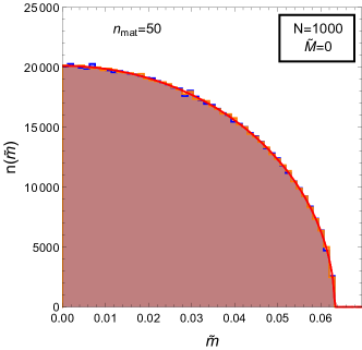
In Fig. 1, we show the density-of-states function for the ensemble constituents generated by diagonalizing randomly generated mass matrices, for and . The blue histogram corresponds to the case, while the orange histogram corresponds to the case. In each case, the results correspond to a data set comprising the ensemble-constituent masses obtained for a sample of randomly generated matrices. By contrast, the red curve in Fig. 1 represents the analytical function in Eq. (22). As evident from Fig. 1, the function provides an excellent approximation to the histogram data, as claimed. Moreover, for such a large value of , the functions and are essentially indistinguishable from . Thus all three functions do an excellent job of approximating the data for .
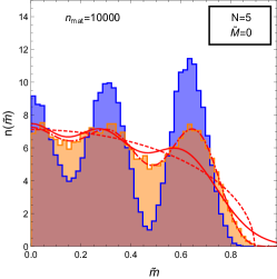
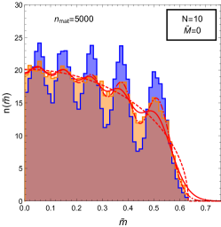
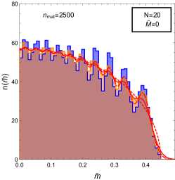
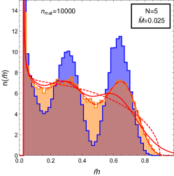
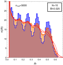
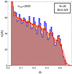
It is also interesting to examine how the results are modified in the regime in which is small and the Wigner semicircle distribution provides a less reliable approximation for the true density of states for the ensemble. In Fig. 2, we show the corresponding results for (left panel), (center panel), and (right panel). In each panel, the blue and orange histograms each represent a data set comprising the ensemble-constituent masses obtained for a sample of randomly generated matrices, where is chosen in each case such that the total number of individual mass eigenvalues in the data set is . As in Fig. 1, the blue histogram corresponds to a model in which the symmetry group is while the orange histogram corresponds to a model in which the symmetry group is . The solid, dot-dashed, and dashed curves in each panel correspond to , , and , respectively.
We see from Fig. 2 that aptly characterizes the overall “envelope” of the true density of states for small in both the and cases, just as it does for large . However, for small , the true density of states for these cases also exhibits oscillations around this envelope — oscillations which grow increasingly pronounced with decreasing . For the case in which the symmetry group is , the histogram data are distributed according to the density-of-states function , as expected; this function actually includes the oscillations, and the histogram differs from only because of random fluctuations. However, for the case in which the symmetry group is , the amplitude of the oscillations is significantly more pronounced, and we see that neither nor are accurate descriptions of the density of states for the case of an symmetry group at small . However, as grows larger (as illustrated in the right panel of Fig. 2), the oscillations fade away in relative magnitude for both the and cases, and the actual distributions qualitatively begin to approach .
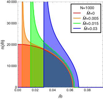
We now turn to consider how the density of states for our ensemble depends on . In Fig. 3, we display curves of the Wigner density-of-states function for different values of . For each of these curves, we have taken — a suitably large value of for which this function provides an excellent approximation to the exact density-of-states function , in the case of either a or symmetry group. We see that for , the presence of the additional contribution to the mass matrix in Eq. (4) distorts the density-of-states function away from the semicircle form which arises in the case. This is simply a reflection of the fact that states in the ensemble which receive comparatively small contributions to their squared masses from symmetry breaking will have masses .
In Fig. 4, we show the corresponding densities of states (similar to Fig. 2) for smaller values of but non-zero . These results exhibit the same qualitative behavior as in Fig. 2.
The main results of this section thus far can be summarized as follows. We have shown that in scenarios in which the ensemble constituents are the component fields of a multiplet which transforms under a spontaneously-broken symmetry group, the PDF for the masses of those constituents takes a well-defined form. As the number of component fields in the multiplet increases, the density-of-states function for our ensemble becomes overwhelmingly statistically likely to coincide with that PDF. Moreover, the properties of this PDF function for the density of states are also significant. In particular we observe that the density-of-states function generally decreases with increasing , and does so in a predictable way with a well-defined upper limit beyond which . By contrast, other natural scenarios which naturally give rise to large numbers of dark particles, such as Kaluza-Klein towers DDM1 ; DDM2 , bound-state resonances in strongly coupled theories DDMString , or oscillator states of a fundamental string DDMString give rise to density-of-state functions which are either independent of or else rise exponentially with .
The emergent mass spectrum we have found in this section is ultimately the hallmark of the underlying randomness within our toy model. Indeed, this behavior for the emergent mass spectrum — and the Wigner semi-circle rule from which it is derived — apply more generally to large classes of random matrices Mehta , only one example of which we have focused on here.
Finally, before concluding this section, it is important to realize that we have only partially tackled the central problem that we face when discussing our random dark sector. Thus far, we have focused on the extent to which a collection of matrices, each yielding eigenvalues, together produce a set of eigenvalues which match our expected “emergent” eigenvalue distributions. This was done holding fixed, so that larger values of required fewer random matrices.
This is fine for a mathematical study of random matrices. However, for practical purposes, the physics question we wish to address is somewhat different. Given the fact that we have only one observable universe, we expect to see only one possible mass spectrum for our DDM ensemble. In other words, although the underlying symmetry-breaking process is random, in reality we expect to get only one “roll of the dice”. Thus, the real question we need to face has to do with the extent to which a given single roll of the dice — i.e., the extent to which a single randomly-generated matrix — generates eigenvalues matching the expected eigenvalue-distribution function . This is similar to the mathematical question we have already studied except that we now wish to hold .
To study this question for any , we randomly generate an matrix following the procedures outlined above, and calculate its eigenvalues. We then place these eigenvalues into bins of equal size based on their magnitudes, and calculate the goodness-of-fit statistic
| (23) |
where labels the bin, where indicates the total number of bins, where is the “observed” number of eigenvalues in the bin, and where is the “expected” number of eigenvalues in the bin according to the eigenvalue-distribution function. Given that we do not have an analytic form for , we obtain our values of via the methods outlined above, choosing a value of for each such that a suitably large total number of random eigenvalues are generated.
The value of in Eq. (23) represents the extent to which the eigenvalues of a single randomly-generated matrix match , as desired. Of course, depending on the particular matrix generated, the corresponding could have values which are extremely large or extremely small. What interests us is therefore , i.e., the average value that might have if we repeat this process times. To help us interpret the result, we then calculate a Gaussian-equivalent significance by comparing to a -distribution with degrees of freedom in order to obtain a -value, and then asking to what statistical significance this -value would correspond for a Gaussian distribution. This value of thus represents the degree to which, on average, the eigenvalues from a single random matrix seem not to have been drawn from the expected distribution. A lower significance thus indicates better agreement with our expectations.
Our results are shown in Fig. 5 for the case of , , and . We have also taken . Note that none of the qualitative results in this figure would change significantly if other values were chosen. We also remark that when establishing our bins, we have we have assumed an eigenvalue range from to , where is the maximum possible eigenvalue that can be obtained for the Wigner semicircle distribution for that same value of . Although eigenvalues values larger than are possible for the true ensemble, we have already seen that such eigenvalues are exceedingly rare and populate a low-statistics regime in which the “expected” bin population is extremely small. Including data in this regime therefore tends to skew the statistics in non-meaningful ways.
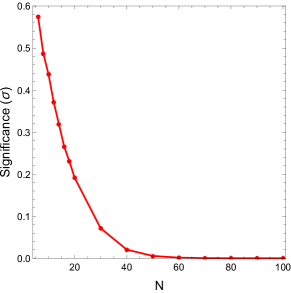
Several features are immediately clear from Fig. 5. As expected, we see that decreases with increasing , indicating that our distributions — oscillations and all — become increasingly precise as grows large. In fact, given the results in Fig. 5, we find that
| (24) |
We thus see that the accuracy of our emergent mass distribution actually grows exponentially with . But perhaps most importantly, we see that our values are themselves extremely small throughout the range of plotted, even for which are relatively small. Thus we can conclude that our emergent eigenvalue distributions do an extremely good job of describing the distributions of masses across the dark sector — even if the symmetries governing the dark sector are not overwhelmingly large.
IV Towards a DDM Ensemble: Couplings, Decay Widths, and Cosmological Abundances
In the previous section, we analyzed the emergent mass spectrum for the example model presented in Sect. II and showed that for the density-of-states function for the converges to the Wigner semicircle function given in Eq. (22). However, in order for these particles to constitute a viable DDM ensemble, they must collectively manifest an appropriate balancing between decay widths and abundances. In this section, we discuss how a spectrum of decay widths and abundances can be generated for the and how the interplay between the corresponding scaling relations and the density-of-states function derived in the previous section can give rise to a DDM-like balancing between decay widths and abundances across the ensemble as a whole. Indeed, as we shall see, a density-of-states function which decreases with the mass — as emerges for our random ensemble — can accommodate a broader range of scaling relations between decay width and mass, and between abundance and mass, than is possible for other distributions.
Note that here and in the following, indices now label the different mass eigenstates .
IV.1 Dark-Matter Decay
We begin with a discussion of the decay properties of the ensemble constituents. The toy model introduced in Sect. II involves only two additional matter fields beyond those of the SM: the multiplets and . Given the symmetry structure of the model, these fields couple to the fields of the SM only via gravitational interactions. Moreover, the symmetry of the model forbids all scattering and decay processes wherein number of particles in the initial and final states differ by an odd number. As a consequence, the lightest of the is absolutely stable. Furthermore, the decay widths of the heavier ensemble constituents are typically dominated by intra-ensemble decays — i.e., decays to final states involving other, lighter . The most relevant intra-ensemble decay processes include , , and, in cases in which the symmetry is local, , where denotes one of the gauge fields.
While channels of this sort provide a natural decay mechanism for the ensemble constituents within the context of this minimal statistical DDM model, these channels are phenomenologically problematic for two reasons. First, the corresponding decay widths are typically far too large. Second, because the final states consist solely of hidden-sector particles, these decays are essentially invisible and yield no observable indirect detection signals. Thus, in order to ensure phenomenological viability, we must find a way to suppress these contributions while at the same time arranging additional mechanisms through which the can decay.
The simplest and most natural way of suppressing processes involving or in the final state is to arrange for the masses of the to be parametrically small in comparison with the masses of the and . Indeed, this is not difficult to arrange. The overall mass scale for the is determined by the mass parameter in Eq. (2) and by the parameter combination . By contrast, the overall mass scales for the and the are both independent of and . Thus, suppressing decays such as and is simply a matter of taking and to be sufficiently small. Indeed, this parametric separation is analogous to the situation in the SM lepton sector, where Majorana masses and Yukawa couplings of the light fermions play the roles of and , respectively.
Intra-ensemble decay processes such as , in which one of the decays to a final state involving only other, lighter ensemble constituents, can also naturally be suppressed in a number of ways. First of all, contributions to such processes which arise due to the quartic interaction in Eq. (2) can be suppressed simply by taking the coupling coefficient , which plays no other important role in the phenomenology of the model, to be sufficiently small. Moreover, the remaining contributions, which proceed via diagrams involving virtual or fields, can likewise be suppressed by taking and to be sufficiently small. Alternatively, intra-ensemble decay processes of this sort can also be forbidden simply by kinematical considerations. For example, processes of the form are kinematically forbidden unless , where is the mass of the lightest ensemble constituent. If the mass spectrum of the theory is such that this condition is not satisfied for even the heaviest of the , such intra-ensemble decays cannot occur. This is not difficult to arrange. Indeed, is essentially determined by , while the splitting between the masses of the heaviest and lightest of the ensemble constituents is essentially determined by ; thus, the lightest mass and the largest mass splitting are parametrically independent.
Having discussed how contributions from processes such as , , and to the decay widths of the can be suppressed, we now turn to examine how decay widths of the correct order of magnitude can be generated for these fields. For concreteness, we present an example of how the ensemble constituents can be coupled to the fields of the SM — and in particular the photon field. We emphasize that this is merely one example, and that other self-consistent coupling scenarios which lead to alternative decay phenomenologies for the are possible as well.
As discussed above, our first step is to break the symmetry. In order to do this in a controlled manner, we introduce an additional field which is odd under and transforms in the fundamental representation of . Given the symmetry structure of the visible and hidden sectors, the simplest method of coupling the to the photon field is via an effective operator of the form
| (25) |
where is the field-strength tensor for the SM photon field, where is the cutoff scale of the effective theory, and where is a dimensionless operator coefficient.
We shall assume that acquires a VEV due to some additional dynamics. Provided that this dynamics is uncorrelated with the dynamics which gives rise to the mass matrix for the , the direction of this VEV in field space is arbitrary. For convenience, we choose to parametrize the VEVs of the individual components of (in the mass eigenbasis of the ) as
| (26) |
Here, the different are dimensionless and subject to the constraint
| (27) |
Note that since the characterize the direction of the VEV in field space, all of them are generically non-zero. By contrast, is a parameter with dimensions of mass which characterizes the overall magnitude of the collective contribution to the breaking of and from the . Since the results derived in Sect. III are predicated on the being the dominant source of symmetry-breaking, we require that . Moreover, as discussed in greater detail below, controls the strength of the effective couplings between the ensemble constituents and the photon field, and therefore the lifetimes of these constituents. Thus, phenomenological considerations associated with dark-matter decay — including, at the very least, the requirement that the longest-lived particle in the ensemble have a lifetime that exceeds the present age of the universe — likewise constrain to be quite small.
Expanding the around their VEVs in Eq. (25) yields an effective tree-level interaction between each of the ensemble constituents and a pair of photons:
| (28) |
Note that in principle, the generically breaks any remaining continuous symmetries under which the are charged, including the residual symmetry associated with phase rotations of each complex scalar . As a result, the generically break the degeneracy between the real and imaginary components of each . Thus, in principle, these degrees of freedom should be treated as distinct real fields. However, because the induced mass splitting between these fields is proportional to , which is constrained to be small in comparison with the masses of the , as discussed above, this splitting has a negligible effect on the mass spectrum of the theory. Therefore, in practice, we may safely neglect the splitting between the real and imaginary parts of the and continue to treat the ensemble constituents as complex fields in what follows.
Under the assumption that the operator in Eq. (28) provides the leading contribution to the decay width of each ensemble constituent , the decay rate of each component is then given by
| (29) |
It is noteworthy that the effect of the randomness in these decay widths is reflected in the coefficients which in turn must satisfy the constraint in Eq. (27). This indicates that while randomness can produce fluctuations in the sizes of these decay widths, these decay widths must nevertheless satisfy the bound
| (30) |
These decay widths therefore cannot grow without limit. As a result, by adjusting the parameters in Eq. (30), it is possible to ensure that our ensemble does not violate observational limits on dark-matter decays to photons (see, e.g., Ref. Slatyer:2012yq ) — all despite the inherent randomness introduced into the decay widths through the coefficients .
IV.2 Annihilation and Abundances
A number of mechanisms exist through which a spectrum of primordial abundances for a set of dark-sector particles can be established. For concreteness, we focus here on one particular mechanism, namely a variation DesigningDDMPaper of thermal freeze-out which yields particularly interesting scaling relations between the masses and abundances of ensemble constituents.
The spectrum of primordial abundances for the depends principally on the masses of these particles and on the cross-sections for the processes through which they annihilate. One of the simplest ways of arranging a set of cross-sections of the correct order of magnitude is to introduce DesigningDDMPaper an additional dark fermion with a mass into which the can annihilate (where is the mass of the lightest ensemble constituent), as well as an additional Abelian gauge group under which both and the multiplet are charged. For phenomenological reasons, we shall also assume that is broken by some additional dynamics, and therefore that the gauge field is massive. In what follows, we shall assume that the breaking of this symmetry is essentially unrelated to the breaking of . In other words, we shall assume that the Goldstone boson which provides the longitudinal polarization of transforms as a singlet under . Under this assumption, all components of will have identical charges and the couplings between and the mass eigenstates may be taken to be diagonal.
In this scenario, the cross-section for dark-matter annihilation processes of the form receives a contribution from diagrams involving an -channel , whereas the cross-section for coannihilation processes of the form with receives no such contribution. Contributions to the cross-sections for annihilation process of the form with (also involving an -channel ) are also generated. Moreover, contributions to the cross-sections for processes of the form are generated for ensemble constituents with directly from the corresponding gauge-kinetic terms in the field Lagrangian. However, in situations in which the effective coupling between and the field is much larger than the coupling between and , the process will dominate. We shall henceforth assume that for all , and thus that the process provides the dominant contribution to the annihilation cross-section of all of the . Moreover, we shall also take and in order to ensure that the annihilation process remains perturbative at all relevant scales.
Under these assumptions, the thermally averaged annihilation cross-section for each ensemble constituent is entirely determined by the masses , , and the couplings , . Following the analysis of Ref. DesigningDDMPaper , we find that the corresponding thermal contribution to the relic abundance of each ensemble constituent takes the form
| (31) |
Alternatively, the may be expressed in terms of the mass , abundance , and coupling of the lightest ensemble constituent. The result is
| (32) |
We emphasize that in this expression the subscript ‘0’ is merely shorthand for that value of for which is minimized.
In interpreting the result in Eq. (32), it is instructive to consider the case in which the couplings between and all of the are identical — i.e., the case in which for all . Thus, as discussed in Ref. DesigningDDMPaper , we see that in the limit in which , the abundance increases with the mass of the ensemble constituent. In particular, . By contrast, in the opposite limit in which , we see that . Thus, in this limit, the heavier ensemble constituents have smaller abundances. Finally, we note that in the special case in which and annihilation of a particular ensemble constituent occurs on resonance, we obtain , where is the total decay width of .
IV.3 Random Ensembles as DDM Ensembles
We now seek to determine whether the scaling relations we have found for our random ensemble are consistent with the phenomenological balancing requirements that are the cornerstone of the DDM framework. As discussed in Refs. DDM1 ; DDM2 , these balancing requirements may be expressed as follows. First, we use our relation between decay widths and masses in order to express our abundance function and density-of-states function in terms of rather than . Note that while and are each densities per unit mass, what we now seek are the corresponding densities and per unit decay width:
| (33) |
Given these new functions, it was then shown in Ref. DDM1 that if scales with according to for some scaling coefficient , and if for some scaling coefficient , then the requirement
| (34) |
serves as a good rudimentary criterion for assessing whether decay widths are balanced against abundances in the appropriate manner to yield a viable DDM ensemble.
For the random toy model we have presented here, the abundance function and density-of-states function , expressed as functions of the constituent mass , are given in Eqs. (32) and (22) for , respectively. Likewise, the result in Eq. (29) implies that , whereupon we see that . As discussed above, in the limit; thus in this limit we have and . We therefore find for this toy model. By contrast, the density-of-states function for the Wigner semicircle distribution which emerges for large does not scale with according to a power law with a constant index , but rather according to a relation with a variable index . Since decreases monotonically with , this variable index is bounded from above: . This implies a corresponding bound on the variable index . Our random toy model therefore has
| (35) |
and this satisfies Eq. (34) for all values of . We thus conclude that our random ensemble indeed displays an appropriate balancing between lifetimes and abundances, as needed in order to serve as a potentially viable DDM ensemble.
It is important to note that this success is not merely restricted to situations in which our decay widths are dominated by dimension-five operators, such as we have considered above. In general, if is the dimension of the dominant decay operator and the daughter particles are light, dimensional analysis implies that . Repeating the above steps assuming then yields and , whereupon we see that , exactly as before. Thus the suitability of our random ensemble to serve as a DDM ensemble is a fairly robust phenomenon.
A few additional comments are in order. First of all, while we have taken the field into which the ensemble constituents annihilate to be a dark-sector fermion for concreteness, there is nothing special about this choice. For example, essentially none of our results would change were we to have taken to be a scalar. Indeed, the result in Eq. (32) does not depend on the spin of . Since the coupling is independent of , the scaling of with is determined by dimensional analysis alone. Moreover, need not be a dark-sector particle at all. For example, a SM fermion could potentially play the role of , provided that phenomenological constraints from indirect detection, collider physics, etc., are satisfied.
Finally, we observe that it is possible to get a sense of the overall mass scale for the DDM ensemble constituents for which a thermal relic density can be successfully obtained by analogy with the case of a standard WIMP. Once again, we focus our attention on the perturbative regime and take for all , so that . In the limit in which and the masses of the are approximately degenerate — i.e., for all — we find that the total abundance of the ensemble takes the form
| (36) |
For a standard WIMP which receives its abundance via thermal freeze-out, the usual constraint that arises due to the requirement that the annihilation cross-section be perturbative is GriestMassLimit . The corresponding constraint on a DDM ensemble of this sort in the degenerate limit in which the are approximately equal becomes
| (37) |
V Indirect-Detection Signals
We now discuss one possible observational signal which arises in this DDM scenario. In particular, we examine the spectrum of high-energy photons produced by the annihilation and decay of the . In principle, contributions to the photon spectrum can arise in this model both from the dark-matter decay process and from the annihilation process , followed by the decay of and and into SM particles. For simplicity, because the annnihilation contribution depends on additional model inputs not directly related to the decay widths or abundances of the — and, in particular, on the decay properties of — we concentrate on the decay contribution.
Under the assumption that the operator in Eq. (28) dominates the width of each of the , the primary injection spectrum of photons from dark-matter decay — i.e., the differential photon flux per unit energy , including the individual contributions from all ensemble constituents — takes the form
| (38) |
The overall normalization of this injection spectrum depends on the astrophysical properties of the object(s) under observation. Interesting possibilities might include, e.g., the galactic center and the halos of Milky-Way dwarf galaxies. However, we can assume that the local energy densities of the within the object(s) under study are proportional to the corresponding cosmological energy densities . In this case, the shape of the injection spectrum depends on particle-physics considerations alone.
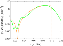
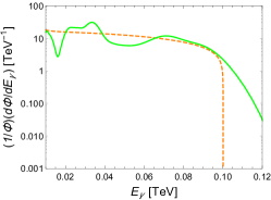
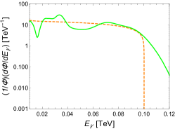
We now illustrate the qualitative features which arise in the photon spectrum of scenarios of this sort. In Fig. 6, we display the contribution to the photon flux from decay in a set of benchmark DDM models with , GeV, and TeV. The left, center, and right panels of Fig. 6 correspond to gauge-boson masses of GeV, TeV, and TeV, respectively, where these masses enter into the calculation of the cosmological abundances in Eq. (38). The green curve in each panel represents one possible spectrum of signal events which might be observed by a gamma-ray detector with a Gaussian energy resolution , given the inherent randomness in the mass matrix and the coupling parameters . Note that we have normalized each spectrum shown such that the total area under the curve is unity. By contrast, the orange curve shown in each panel represents the corresponding injection spectrum obtained by taking the analytic expression for as the density of states for the ensemble, and by taking a universal coupling between each and the photon field, all while ignoring detector effects. Thus, the orange curve can be viewed as representing the overall reference “baseline” around which the corresponding actual injection spectrum fluctuates due to the inherent randomness in the masses and couplings.
The gamma-ray spectra shown in Fig. 6 display a number of distinctive features. One such feature is the characteristic shape of the spectral baseline (i.e., the orange curve), which is primarily determined by the density-of-states function for our statistical DDM ensemble. Indeed, in the center and right panels of the figure, the influence of this density-of-states function on the spectral envelope is unmistakable. In the left panel, which corresponds to the case in which GeV, the shape of the envelope is modified at energies around GeV due to the effect of the annihilation resonance, which suppresses the abundances (and therefore the photon-flux contributions) of ensemble constituents with masses GeV. Nevertheless, even in this case, the influence of the density-of-states function on the spectral baseline is still evident — especially at large .
Another distinctive feature which emerges in the gamma-ray spectra of statistical DDM ensembles is the pattern of fluctuations in the observed spectrum around the spectral baseline. Indeed, in the regime in which the scale of the splitting between the exceeds the energy resolution of the detector, significant fluctuations are apparent across the relevant range of . These fluctuations (along with detector effects) can obscure features which would otherwise be apparent in the gamma-ray spectrum. For example, the pronounced dip in the spectral baseline due to the annihilation resonance is only partially evident in the observed gamma-ray spectrum for the corresponding DDM ensemble. By contrast, we see that in the regime in which is large and the energy resolution of the detector is less than or comparable to the rough scale of the splitting between the mass eigenvalues , the effect of the random alignment of the is smeared out by detector effects. Consequently, in this regime, the observed spectrum is reasonably well approximated by the spectral baseline up to the cutoff at GeV, which corresponds to the upper limit of the Wigner-Semicircle distribution for this choice of parameters. The divergence between the observed spectrum and the spectral baseline above this cutoff is solely a result of detector smearing.
We note that the flux spectrum shown in left panel of Fig. 6 displays fluctuations with magnitudes as large as 50% or more of the overall baseline. This is comparable to the fractional uncertainty in the measurement of the isotropic diffuse gamma-ray background at GeV Ackermann:2014usa . This implies that the potentially identifiable signals of statistical DDM ensembles of this sort may manifest themselves not only in the distinctive shape of the overall baseline associated with the gamma-ray spectrum, but also in the pattern of fluctuations in that spectrum.
VI Conclusions
In this paper, we studied the possibility that the properties of the dark sector are dominated by processes which are essentially random. We considered a dark sector composed of an ensemble of individual components with differing masses, cosmological abundances, and couplings to the SM, and constructed a toy model in which the mass spectrum associated with this ensemble is determined through an essentially random breaking of an internal dark-sector symmetry. Even though this mass spectrum is determined randomly, we were nevertheless able to bring the machinery of random-matrix theory to bear in order to derive predictions for the probability distribution of mass eigenvalues for these component fields. In this way, we were able to obtain a statistical prediction for a density-of-states function for the ensemble as a whole — a prediction which grows more and more robust as the number of ensemble constituents increases. Moreover, we found that this emergent density of states decreases as a function of mass and actually has an upper limit beyond which — behavior which is quite unlike the density-of-states functions for all other DDM ensembles which have previously been discussed in the literature.
Given these results for the dark-sector mass spectrum, we then proceeded to demonstrate that a set of corresponding cosmological abundances and decay widths for the ensemble constituents can be generated via well-established mechanisms — thermal freeze-out and the controlled breaking of a stabilizing symmetry, respectively. We then found that in scenarios of this sort, the fundamental scaling relations which govern the ensemble satisfy the basic criteria to be interpreted as potentially viable DDM ensembles — ensembles in which cosmological abundances and decay widths satisfy certain balancing relations across all constituents. Thus, we were able to demonstrate that randomness in the dark sector coexists quite naturally with DDM. Finally, we explored one possible observational signature of random DDM ensembles of this sort, namely the indirect detection of high-energy gamma rays produced from the decays of the ensemble constituents, and evaluated the prospects for the detection of such signals.
There are many ways in which the analysis of this paper might be generalized and extended. As we have discussed in the Introduction, there are three aspects of a dark-sector ensemble which are critical in determining the resulting phenomenology: the spectrum of constituent masses, the spectrum of constituent cosmological abundances, and the spectrum of constituent decay widths into SM states. While the first of these describes the properties of the ensemble unto itself, the second and third depend upon further information concerning how the ensemble emerges within a particular cosmological history and/or couples to SM states. In this paper, we investigated the case in which only the first of these — namely the mass spectrum — is determined randomly. Indeed, as have seen, the simple random mechanism which gives rise to the density-of-states function for our ensemble is essentially unrelated to the physics which determines the abundances and decay widths of the ensemble constituents.
Given this, we may view our random mechanism as a fundamental “kernel” for establishing an ensemble with a particular density-of-states function, a kernel which can be incorporated as an ingredient in any number of alternative scenarios. As discussed in Sect. III, the fact that the density of states for such ensembles decreases with increasing implies that this “kernel” should be compatible with a wide variety of scenarios for abundance and decay-width generation. Indeed, a broad class of models could be developed around ensembles of this sort whose detailed phenomenological implications might exhibit interesting and unanticipated characteristics. It would also be interesting to explore further scenarios in which the mechanisms for generating cosmological abundances and SM decay widths are themselves based on random processes.
It would also be interesting to consider more broadly the methods by which randomness in the dark sector might be detected. Identifying characteristic features in the gamma-ray spectra of those statistical DDM ensembles, as we have discussed in Sect. V, may represent only one possible way of distinguishing between such ensembles experimentally. Such ensembles clearly have a rich phenomenology and could potentially give rise to characteristic signals in the kinematic distributions of event-shape variables at colliders and as well as in distinctive recoil-energy spectra observed at direct-detection experiments.
Finally, near the end of Sect. III, we stated that a single universe can only exhibit one mass spectrum for the dark sector. In other words, as stated there, we get only “one roll of the dice”. Of course, there are certain situations in which this is not strictly true. For example, if the random effects which ultimately give rise to our dark-sector mass spectrum are associated with a first-order symmetry-breaking phase transition, then different regions of spacetime could each correspond to their own distinct roll of the dice. Likewise, multiple rolls of the dice could also arise if we live a full-fledged multiverse, as recent developments in string theory suggest. These questions are especially critical in the case of differing dark sectors because the dark sector carries a significant matter-based energy density and thus its properties play a major role in the time evolution of the universe.
In either case, however, the end result would be a series of different universes (or regions of spacetime) with different dark sectors, each existing within its own spatial domain and separated from the others by domain walls. Such domain-wall topological defects would undoubtedly give rise to dramatic effects of their own, even beyond those associated with the properties of the different dark sectors they separate, and consequently there are tight phenomenological and astrophysical/cosmological constraints that can already be placed on such scenarios coming from CMB anistropy limits and other energy-density constraints. However, if the only differences between the different universes are those that result from different random throws of the -breaking dice in the dark sector, then the probability distribution functions we have discussed in this paper might have an even greater relevance than we have imagined here, as averages across the entire universe or multiverse as a whole.
Acknowledgements.
We would like to thank Jonathan Feng and Shrihari Gopalakrishna for useful discussions. KRD is supported in part by the Department of Energy under Grant DE-FG02-13ER41976 and by the National Science Foundation through its employee IR/D program. JK is supported in part by NSF CAREER grant PHY-1250573. BT is supported in part by an internal research award from Reed College. KRD, JK, and BT would also like to thank the Center for Theoretical Underground Physics and Related Areas (CETUP∗) in Lead, South Dakota, for hospitality during the 2015 Summer Program. The opinions and conclusions expressed herein are those of the authors, and do not represent any funding agencies.References
- (1) K. R. Dienes and B. Thomas, Phys. Rev. D 85, 083523 (2012) [arXiv:1106.4546 [hep-ph]].
- (2) K. R. Dienes and B. Thomas, Phys. Rev. D 85, 083524 (2012) [arXiv:1107.0721 [hep-ph]].
- (3) K. R. Dienes and B. Thomas, Phys. Rev. D 86, 055013 (2012) [arXiv:1203.1923 [hep-ph]].
- (4) K. R. Dienes, S. Su and B. Thomas, Phys. Rev. D 86, 054008 (2012) [arXiv:1204.4183 [hep-ph]].
- (5) K. R. Dienes, J. Kumar and B. Thomas, Phys. Rev. D 86, 055016 (2012) [arXiv:1208.0336 [hep-ph]].
- (6) K. R. Dienes, J. Kumar and B. Thomas, Phys. Rev. D 88, 103509 (2013) [arXiv:1306.2959 [hep-ph]].
- (7) K. R. Dienes, S. Su and B. Thomas, Phys. Rev. D 91, 054002 (2015) [arXiv:1407.2606 [hep-ph]].
- (8) K. R. Dienes, J. Kumar, B. Thomas and D. Yaylali, Phys. Rev. Lett. 114, 051301 (2015) [arXiv:1406.4868 [hep-ph]].
- (9) K. R. Dienes, J. Kost and B. Thomas, arXiv:1509.00470 [hep-ph] (to appear in Phys. Rev. D).
- (10) K. R. Dienes, F. Huang, S. Su, and B. Thomas, to appear.
- (11) K. R. Dienes, J. Fennick, J. Kumar, and B. Thomas, to appear.
- (12) P. A. R. Ade et al. [Planck Collaboration], arXiv:1502.01589 [astro-ph.CO].
- (13) L. Ackerman, M. R. Buckley, S. M. Carroll and M. Kamionkowski, Phys. Rev. D 79, 023519 (2009) [arXiv:0810.5126 [hep-ph]].
- (14) M. L. Mehta, Random Matrices (3rd ed.), Amsterdam, Elsevier/Academic Press, 2004.
- (15) S. Lloyd and H. Pagels, Ann. Phys. 188 186 (1988).
- (16) K. Zyczkowski and H. Sommers, J. Phys. A 34 7111 (2001).
- (17) G. Akemann, G. M. Cicuta, L. Molinari, and G. Vernizzi, Phys. Rev. E 59 1489 (1999).
- (18) R. Delannay and G. Le Caër, J. Phys. A 33 2611 (2000).
- (19) E. Wigner, Annals Math. 62, 548 (1955); Annals Math. 67, 325 (1958).
- (20) T. R. Slatyer, Phys. Rev. D 87, 123513 (2013) [arXiv:1211.0283 [astro-ph.CO]].
- (21) K. Griest and M. Kamionkowski, Phys. Rev. Lett. 64, 615 (1990).
- (22) M. Ackermann et al. [Fermi-LAT Collaboration], Astrophys. J. 799, 86 (2015) [arXiv:1410.3696 [astro-ph.HE]].