PupilNet: Convolutional Neural Networks for Robust Pupil Detection

Abstract

Real-time, accurate, and robust pupil detection is an essential prerequisite for pervasive video-based eye-tracking. However, automated pupil detection in real-world scenarios has proven to be an intricate challenge due to fast illumination changes, pupil occlusion, non centered and off-axis eye recording, and physiological eye characteristics. In this paper, we propose and evaluate a method based on a novel dual convolutional neural network pipeline. In its first stage the pipeline performs coarse pupil position identification using a convolutional neural network and subregions from a downscaled input image to decrease computational costs. Using subregions derived from a small window around the initial pupil position estimate, the second pipeline stage employs another convolutional neural network to refine this position, resulting in an increased pupil detection rate up to 25% in comparison with the best performing state-of-the-art algorithm. Annotated data sets can be made available upon request.

1 Introduction

For over a century now, the observation and measurement of eye movements have been employed to gain a comprehensive understanding on how the human oculomotor and visual perception systems work, providing key insights about cognitive processes and behavior [32]. Eye-tracking devices are rather modern tools for the observation of eye movements. In its early stages, eye tracking was restricted to static activities, such as reading and image perception [33], due to restrictions imposed by the eye-tracking system – e.g., size, weight, cable connections, and restrictions to the subject itself. With recent developments in video-based eye-tracking technology, eye tracking has become an important instrument for cognitive behavior studies in many areas, ranging from real-time and complex applications (e.g., driving assistance based on eye-tracking input [11] and gaze-based interaction [31]) to less demanding use cases, such as usability analysis for web pages [3]. Moreover, the future seems to hold promises of pervasive and unobtrusive video-based eye tracking [14], enabling research and applications previously only imagined.

While video-based eye tracking has been shown to perform satisfactorily under laboratory conditions, many studies report the occurrence of difficulties and low pupil detection rates when these eye trackers are employed for tasks in natural environments, for instance driving [11, 21, 30] and shopping [13]. The main source of noise in such realistic scenarios is an unreliable pupil signal, mostly related to intricate challenges in the image-based pupil detection. A variety of difficulties occurring when using such eye trackers, such as changing illumination, motion blur, and pupil occlusion due to eyelashes, are summarized in [28]. Rapidly changing illumination conditions arise primarily in tasks where the subject is moving fast (e.g., while driving) or rotates relative to unequally distributed light sources, while motion blur can be caused by the image sensor capturing images during fast eye movements such as saccades. Furthermore, eyewear (e.g., spectacles and contact lenses) can result in substantial and varied forms of reflections (Figure 1a and Figure 1b), non-centered or off-axis eye position relative to the eye-tracker can lead to pupil detection problems, e.g., when the pupil is surrounded by a dark region (Figure 1c). Other difficulties are often posed by physiological eye characteristics, which may interfere with detection algorithms (Figure 1d). As a consequence, the data collected in such studies must be post-processed manually, which is a laborious and time-consuming procedure. Additionally, this post-processing is impossible for real-time applications that rely on the pupil monitoring (e.g., driving or surgery assistance). Therefore, a real-time, accurate, and robust pupil detection is an essential prerequisite for pervasive video-based eye-tracking.

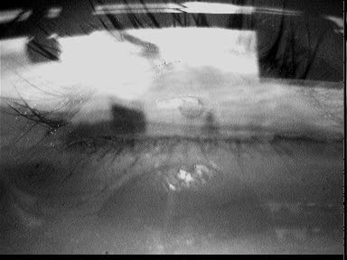
(a)

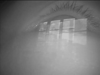
(b)

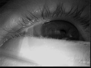
(c)

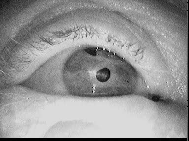
(d)

Figure 1: Images of typical pupil detection challenges in real-world scenarios: (a) and (b) reflections, (c) pupil located in dark area, and (d) unexpected physiological structures.

State-of-the-art pupil detection methods range from relatively simple methods such as combining thresholding and mass center estimation [25] to more elaborated methods that attempt to identify the presence of reflections in the eye image and apply pupil-detection methods specifically tailored to handle such challenges [7] – a comprehensive review is given in Section 2. Despite substantial improvements over earlier methods in real-world scenarios, these current algorithms still present unsatisfactory detection rates in many important realistic use cases (as low as 34% [7]). However, in this work we show that carefully designed and trained convolutional neural networks (CNN) [4, 17], which rely on statistical learning rather than hand-crafted heuristics, are a substantial step forward in the field of automated pupil detection. CNNs have been shown to reach human-level performance on a multitude of pattern recognition tasks (e.g., digit recognition [2], image classification [16]). These networks attempt to emulate the behavior of the visual processing system and were designed based on insights from visual perception research.

We propose a dual convolutional neural network pipeline for image-based pupil detection. The first pipeline stage employs a shallow CNN on subregions of a downscaled version of the input image to quickly infer a coarse estimate of the pupil location. This coarse estimation allows the second stage to consider only a small region of the original image, thus, mitigating the impact of noise and decreasing computational costs. The second pipeline stage then samples a small window around the coarse position estimate and refines the initial estimate by evaluating subregions derived from this window using a second CNN. We have focused on robust learning strategies (batch learning) instead of more accurate ones (stochastic gradient descent) [18] due to the fact that an adaptive approach has to handle noise (e.g., illumination, occlusion, interference) effectively.

The motivation behind the proposed pipeline is (i) to reduce the noise in the coarse estimation of the pupil position, (ii) to reliably detect the exact pupil position from the initial estimate, and (iii) to provide an efficient method that can be run in real-time on hardware architectures without an accessible GPU.

In addition, we propose a method for generating training data in an online-fashion, thus being applicable to the task of pupil center detection in online scenarios. We evaluated the performance of different CNN configurations both in terms of quality and efficiency and report considerable improvements over stat-of-the-art techniques.

2 Related Work

During the last two decades, several algorithms have addressed image-based pupil detection. Pérez et al. [25] first threshold the image and compute the mass center of the resulting dark pixels. This process is iteratively repeated in an area around the previously estimated mass center to determine a new mass center until convergence. The Starburst algorithm, proposed by Li et al. [19], first removes the corneal reflection and then locates pupil edge points using an iterative feature-based approach. Based on the RANSAC algorithm [6], a best fitting ellipse is then determined, and the final ellipse parameters are determined by applying a model-based optimization. Long et al. [22] first downsample the image and search there for an approximate pupil location. The image area around this location is further processed and a parallelogram-based symmetric mass center algorithm is applied to locate the pupil center. In another approach, Lin et al. [20] threshold the image, remove artifacts by means of morphological operations, and apply inscribed parallelograms to determine the pupil center. Keil et al. [15] first locate corneal reflections; afterwards, the input image is thresholded, the pupil blob is searched in the adjacency of the corneal reflection, and the centroid of pixels belonging to the blob is taken as pupil center. Agustin et al. [27] threshold the input image and extract points in the contour between pupil and iris, which are then fitted to an ellipse based on the RANSAC method to eliminate possible outliers. Świrski et al. [29] start with a coarse positioning using Haar-like features. The intensity histogram of the coarse position is clustered using k-means clustering, followed by a modified RANSAC-based ellipse fit. The above approaches have shown good detection rates and robustness in controlled settings, i.e., laboratory conditions.

Two recent methods, SET [10] and ExCuSe [7], explicitly address the aforementioned challenges associated with pupil detection in natural environments. SET [10] first extracts pupil pixels based on a luminance threshold. The resulting image is then segmented, and the segment borders are extracted using a Convex Hull method. Ellipses are fit to the segments based on their sinusoidal components, and the ellipse closest to a circle is selected as pupil. ExCuSe [7] first analyzes the input images with regard to reflections based on intensity histograms. Several processing steps based on edge detectors, morphologic operations, and the Angular Integral Projection Function are then applied to extract the pupil contour. Finally, an ellipse is fit to this line using the direct least squares method.

Although the latter two methods report substantial improvements over earlier methods, noise still remains a major issue. Thus, robust detection, which is critical in many online real-world applications, remains an open and challenging problem [7].

3 Method

The overall workflow for the proposed algorithm is shown in Figure 2. In the first stage, the image is downscaled and divided into overlapping subregions. These subregions are evaluated by the first CNN, and the center of the subregion that evokes the highest CNN response is used as a coarse pupil position estimate. Afterwards, this initial estimate is fed into the second pipeline stage. In this stage, subregions surrounding the initial estimate of the pupil position in the original input image are evaluated using a second CNN. The center of the subregion that evokes the highest CNN response is chosen as the final pupil center location. This two-step approach has the advantage that the first step (i.e., coarse positioning) has to handle less noise because of the bicubic downscaling of the image and, consequently, involves less computational costs than detecting the pupil on the complete upscaled image.

In the following subsections, we delineate these pipeline stages and their CNN structures in detail, followed by the training procedure employed for each CNN.

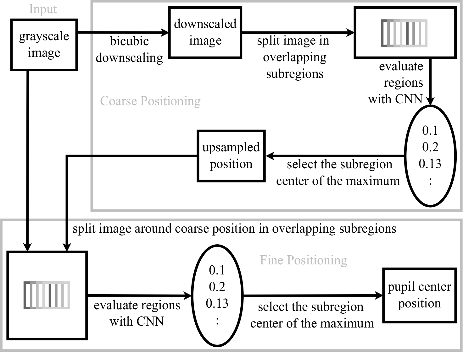
Figure 2: Workflow of the proposed algorithm. First a CNN is employed to estimate a coarse pupil position based on subregions from a downscaled version of the input image. This position is then refined using subregions around the coarse estimation in the original input image by a second CNN.

3.1 Coarse Positioning Stage

The grayscale input images generated by the mobile eye tracker used in this work are sized $384\times 288$ pixels. Directly employing CNNs on images of this size would demand a large amount of resources and would thus be computationally expensive, impeding their usage in state-of-the-art mobile eye trackers. Thus, one of the purposes of the first stage is to reduce computational costs by providing a coarse estimate that can in turn be used to reduce the search space of the exact pupil location. However, the main reason for this step is to reduce noise, which can be induced by different camera distances, changing sensory systems between head-mounted eye trackers [1, 5, 26], movement of the camera itself, or the usage of uncalibrated cameras (e.g., focus or white balance). To achieve this goal, first the input image is downscaled using a bicubic interpolation, which employs a third order polynomial in a two dimensional space to evaluate the resulting values. In our implementation, we employ a downscaling factor of four times, resulting in images of $96\times 72$ pixels. Given that these images contain the entire eye, we chose a CNN input size of $24\times 24$ pixels to guarantee that the pupil is fully contained within a subregion of the downscaled images. Subregions of the downscaled image are extracted by shifting a $24\times 24$ pixels window with a stride of one pixel (see Figure 3a) and evaluated by the CNN, resulting in a rating within the interval [0,1] (see Figure 3b). These ratings represent the confidence of the CNN that the pupil center is within the subregion. Thus, the center of the highest rated subregion is chosen as the coarse pupil location estimation.

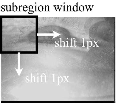
(a)

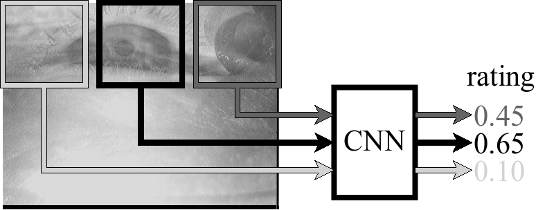
(b)

Figure 3: The downscaled image is divided in subregions of size $24\times 24$ pixels with a stride of one pixel (a), which are then rated by the first stage CNN (b).

The core architecture of the first stage CNN is summarized in Figure 4. The first layer is a convolutional layer with kernel size $5\times 5$ pixels, one pixel stride, and no padding. The convolution layer is followed by an average pooling layer with window size $4\times 4$ pixels and four pixels stride, which is connected to a fully-connected layer with depth one. The output is then fed to a single perceptron, responsible for yielding the final rating within the interval [0,1]. We have evaluated this architecture for different amounts of filters in the convolutional layer and varying numbers of perceptrons in the fully connected layer; these values are reported in Section 5. The main idea behind the selected architecture is that the convolutional layer learns basic features, such as edges, approximating the pupil structure. The average pooling layer makes the CNN robust to small translations and blurring of these features (e.g., due to the initial downscaling of the input image). The fully connected layer incorporates deeper knowledge on how to combine the learned features for the coarse detection of the pupil position by using the logistic activation function to produce the final rating.

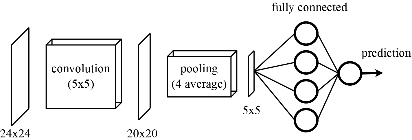
Figure 4: The coarse position stage CNN. The first layer consists of the shared weights or convolution masks, which are summarized by the average pooling layer. Then a fully connected layer combines the features forwarded from the previous layer and delegates the final rating to a single perceptron.

3.2 Fine Positioning Stage

Although the first stage yields an accurate pupil position estimate, it lacks precision due to the inherent error introduced by the downscaling step. Therefore, it is necessary to refine this estimate. This refinement could be attempted by applying methods similar to those described in Section 2 to a small window around the coarse pupil position estimate. However, since most of the previously mentioned challenges are not alleviated by using this small window, we chose to use a second CNN that evaluates subregions surrounding the coarse estimate in the original image.

The second stage CNN employs the same architecture pattern as the first stage (i.e., convolution $\Rightarrow$ average pooling $\Rightarrow$ fully connected $\Rightarrow$ single logistic perceptron) since their motivations are analogous. Nevertheless, this CNN operates on a larger input resolution to provide increased precision. Intuitively, the input image for this CNN would be $96\times 96$ pixels: the input size of the first CNN input ($24\times 24$) multiplied by the downscaling factor ($4$). However, the resulting memory requirement for this size was larger than available on our test device; as a result, we utilized the closest working size possible: $89\times 89$ pixels. The size of the other layers were adapted accordingly. The convolution kernels in the first layer were enlarged to $20$ pixels to compensate for increased noise and motion blur. The dimension of the pooling window was increased by one pixel on each side, leading to a decreased input size on the fully connected layer and reduced runtime. This CNN uses eight convolution filters and eight perceptrons due to the increased size of the convolution filter and the input region size. Subregions surrounding the coarse pupil position are extracted based on a window of size $89\times 89$ pixels centered around the coarse estimate, which is shifted from $-10$ to $10$ pixels (with a one pixel stride) horizontally and vertically. Analogously to the first stage, the center of the region with the highest CNN rating is selected as fine pupil position estimate.

Despite higher computational costs in the second stage, our approach is highly efficient and can be run on today’s conventional mobile computers.

3.3 CNN Training Methodology

Both CNNs were trained using supervised batch gradient descent [18] (which is explained in detail in the supplementary material) with a fixed learning rate of one. Unless specified otherwise, training was conducted for ten epochs with a batch size of 500. Obviously, these decisions are aimed at an adaptive solution, where the training time must be relatively short (hence the small number of epochs and high learning rate) and no normalization (e.g., PCA whitening, mean extraction) can be performed. All CNNs’ weights were initialized with random samples from a uniform distribution, thus accounting for symmetry breaking.

While stochastic gradient descent searches for minima in the error plane more effectively than batch learning [8, 23] when give valid examples, it is vulnerable to disastrous hops if given inadequate examples (e.g., due to poor performance of the traditional algorithm). On the contrary, batch training dilutes this error. Nevertheless, we explored the impact of stochastic learning (i.e., using a batch size of one) as well as an increased number of training epochs in Section 5.

3.3.1 Coarse Positioning CNN

The coarse position CNN was trained on subregions extracted from the downscaled input images that fall into two different data classes: containing a valid ($label=1$) or invalid ($label=0$) pupil center. Training subregions were extracted by collecting all subregions with center distant up to five pixels from the hand-labeled pupil center. Subregions with center distant up to one pixel were labeled as valid examples while the remaining subregions were labeled as invalid examples. As exemplified by Figure 5, this procedure results in nine valid and 32 invalid samples per hand-labeled data.

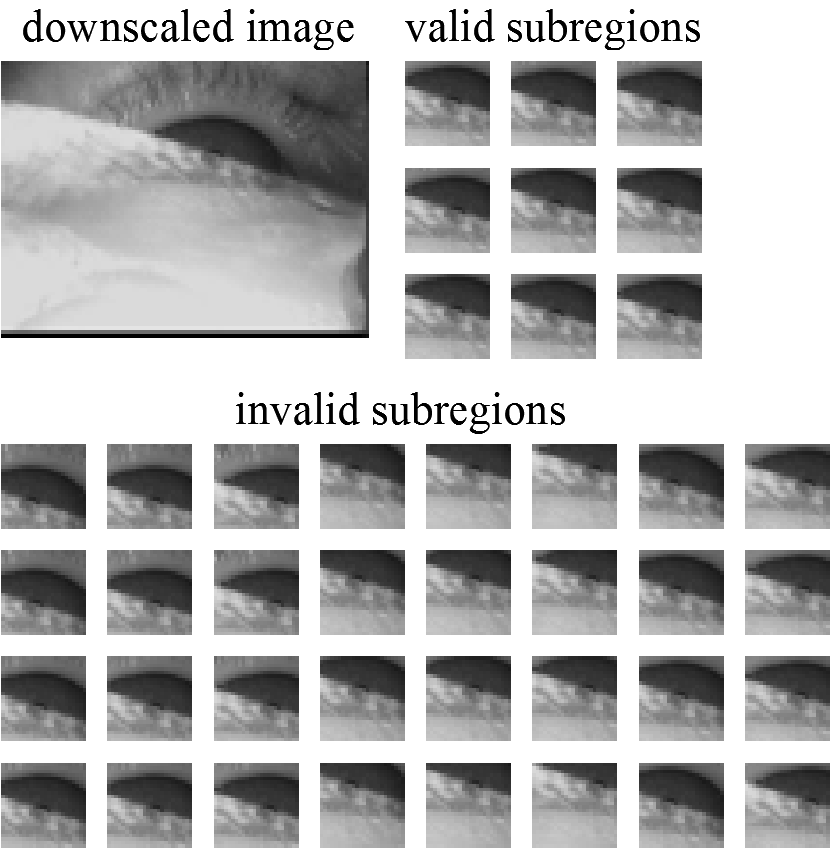
Figure 5: Nine valid (top right) and 32 invalid (bottom) training samples for the coarse position CNN extracted from a downscaled input image (top left).

We generated two training sets for the CNN responsible for the coarse position detection. The first training set consists of 50% of the images provided by related work from Fuhl et al. [7]. The remaining 50% of the images as well as the additional data sets from this work (see Section 4) are used to evaluate the detection performance of our approach. The purpose of this training is to investigate how the coarse positioning CNN behaves on data it has never seen before. The second training includes the first training set and 50% of the images of our new data sets and is employed to evaluate the complete proposed method (i.e., coarse and fine positioning).

3.3.2 Fine Positioning CNN

The fine positioning CNN (responsible for detecting the exact pupil position) is trained similarly to the coarse positioning one. However, we extract only one valid subregion sample centered at the hand-labeled pupil center and eight equally spaced invalid subregions samples centered five pixels away from the hand-labeled pupil center. This reduced amount of samples per hand-labeled data relative to the coarse positioning training is to constrain learning time, as well as main memory and storage consumption. We generated samples from 50% of the images from Fuhl et al. [7] and from the additional data sets. Out of these samples, we randomly selected 50% of the valid examples and 25% of the generated invalid examples for training.

4 Data Set

In this study, we used the extensive data sets introduced by Fuhl et al. [7], complemented by five additional hand-labeled data sets. Our additional data sets include 41,217 images collected during driving sessions in public roads for an experiment [12] that was not related to pupil detection and were chosen due the non-satisfactory performance of the proprietary pupil detection algorithm. These new data sets include fast changing and adverse illumination, spectacle reflections, and disruptive physiological eye characteristics (e.g., dark spot on the iris); samples from these data sets are shown in Figure 6.

Figure 6: Samples from the additional data sets employed in this work. Each column belongs to a distinct data set. The top row includes non-challenging samples, which can be considered relatively similar to laboratory conditions and represent only a small fraction of each data set. The other two rows include challenging samples with artifacts caused by the natural environment.

5 Evaluation

Training and evaluation were performed on an Intel^® Core™i5-4670 desktop computer with 8GB RAM. This setup was chosen because it provides a performance similar to systems that are usually provided by eye-tracker vendors, thus enabling the actual eye-tracking system to perform other experiments along with the evaluation. The algorithm was implemented using MATLAB (r2013b) combined with the deep learning toolbox [24]. During this evaluation, we employ the following name convention: K_n and P_k signify that the CNN has n filters in the convolution layer and k perceptrons in the fully connected layer. We report our results in terms of the average pupil detection rate as a function of pixel distance between the algorithmically established and the hand-labeled pupil center. Although the ground truth was labeled by experts in eye-tracking research, imprecision cannot be excluded. Therefore, the results are discussed for a pixel error of five (i.e., pixel distance between the algorithmically established and the hand-labeled pupil center), analogously to [7, 29].

5.1 Coarse Positioning

We start by evaluating the candidates from Table 1 for the coarse positioning CNN. All candidates follow the core architecture presented in Section 3.1 and each candidate has a specific number of filters in the convolution layer and perceptrons in the fully connected layer. Their names are prefixed with C for coarse and, as previously specified in Section 3.3, were trained for ten epochs with a batch size of 500. Moreover, since $CK_{8}P_{16}$ provided the best trade-off between performance and computational requirements, we chose this configuration to evaluate the impact of training for an extended period of time, resulting in the CNN $CK_{8}P_{16}$$ext$, which was trained for a hundred epochs with a batch size of 1000. Because of inferior performance and for the sake of space we omit the results for the stochastic gradient descent learning but will make them available online.

CNN	Conv. Kernels	Fully Conn. Perceptrons
$CK_{4}P_{8}$	04	08
$CK_{8}P_{8}$	08	08
$CK_{8}P_{16}$	08	16
$CK_{16}P_{32}$	16	32

Table 1: Evaluated configurations for the coarse positioning CNN (as described in Section 3.1).

Figure 7 shows the performance of the coarse positioning CNNs when trained using 50% of the images randomly chosen from all data sets and evaluated on all images. As can be seen in this figure, the number of filters in the first layer (compare $CK_{4}P_{8}$, $CK_{8}P_{8}$, and $CK_{16}P_{32}$) and extensive learning (see $CK_{8}P_{16}$ and $CK_{8}P_{16}$$ext$) have a higher impact than the number of perceptrons in the fully connected layer (compare $CK_{8}P_{8}$ to $CK_{8}P_{16}$). Moreover, these results indicate that the amount of filters in the convolutional layer still has not been saturated (i.e., there are still high level features that can be learned to improve accuracy). However, it is important to notice that this is the most expensive parameter in the proposed CNN architecture in terms of computation time and, thus, further increments must be carefully included.

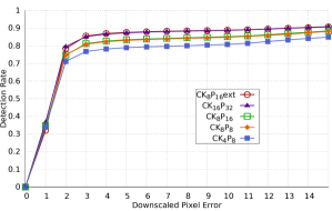
Figure 7: Performance for the evaluated coarse CNNs trained on 50% of images from all data sets and evaluated on all images from all data sets.

To evaluate the performance of the coarse CNNs only on data they have not seen before, we additionally retrained these CNNs from scratch using only 50% of the images in the data sets provided by Fuhl et al. [7] and evaluated their performance solely on the new data sets provided by this work. These results were compared to those from the CNNs that were trained on 50% of images from all data sets and are shown in Figure 8. The CNNs that have not learned on the new data sets are identified by the suffix nl. All nl-CNNs exhibited a similar decrease in performance relative to their counterparts that have been trained on samples from all the data sets. We hypothesize that this effect is due to the new data sets holding new information (i.e., containing new challenging patterns not present in the training data); nevertheless, the CNNs generalize well enough to handle even these unseen patterns decently.

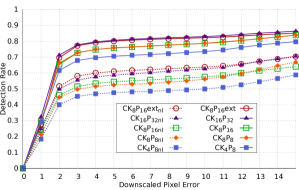
Figure 8: Performance of coarse positioning CNNs on all images provided by this work. The solid lines belong to the CNNs trained on 50% of all images from all data sets. The dotted lines belong to the nl-CNNs, which were trained only on 50% of the data set provided by Fuhl et al. [7] and, thus, have not learned on examples from the evaluation data sets.

5.2 Fine Positioning

The fine positioning CNN ($FK_{8}P_{8}$) uses the $CK_{8}P_{8}$ in the first stage and was trained on 50% of the data from all data sets. Evaluation was performed against four state-of-the-art algorithms, namely, ExCuSe [7], SET [10], Starburst [19], and Świrski [29]. Furthermore, we have developed two additional fine positioning methods for this evaluation:

• $CK_{8}P_{8}$$ray$: this method employs $CK_{8}P_{8}$ to determine a coarse estimation, which is then refined by sending rays in eight equidistant directions with a maximum range of thirty pixels. The difference between every two adjacent pixels in the ray’s trajectory is calculated, and the center of the opposite ray is calculated. Then, the mean of the two closest centers is used as fine position estimate. This method is used as reference for hybrid methods combining CNNs and traditional pupil detection methods.

• $SK_{8}P_{8}$: this method uses only a single CNN similar to the ones used in the coarse positioning stage, trained in an analogous fashion. However, this CNN uses an input size of $25\times 25$ pixels to obtain an even center. This method is used as reference for a parsimonious (although costlier than the original coarse positioning CNNs) single stage CNN approach and was designed to be employed on systems that cannot handle the second stage CNN.

For reference, the coarse positioning CNN used in the first stage of $FK_{8}P_{8}$ and $CK_{8}P_{8}$$ray$ (i.e., $CK_{8}P_{8}$) is also shown.

All CNNs in this evaluation were trained on 50% of the images randomly selected from all data sets. To avoid biasing the evaluation towards the data set introduced by this work, we considered two different evaluation scenarios. First, we evaluate the selected approaches only on images from the data sets introduced by Fuhl et al. [7], and, in a second step, we perform the evaluation on all images from all data sets. The outcomes are shown in the Figures 9a and 9b, respectively. Finally, we evaluated the performance on all images not used for training from all data sets. This provides a realistic evaluation strategy for the aforementioned adaptive solution. The results are shown in Figure 9c.

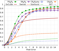
(a)

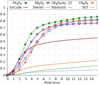
(b)

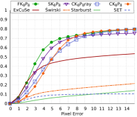
(c)

Figure 9: All CNNs were trained on 50% of images from all data sets. Performance for the selected approaches on (a) all images from the data sets from [7], (b) all images from all data sets, and (c) all images not used for training from all data sets.

In all cases, both $FK_{8}P_{8}$ and $SK_{8}P_{8}$ surpass the best performing state-of-the-art algorithm by approximately 25% and 15%, respectively. Moreover, even with the penalty due to the upscaling error, the evaluated coarse positioning approaches mostly exhibit an improvement relative to the state-of-the-art algorithms. The hybrid method $CK_{8}P_{8}$$ray$, did not display a significant improvement relative to the coarse positioning; as previously discussed, this behavior is expected as the traditional pupil detection methods are still afflicted by aforementioned challenges, regardless of the availability of the coarse pupil position estimate. Although the proposed method ($FK_{8}P_{8}$) exhibits the best pupil detection rate, it is worth highlighting the performance of the $SK_{8}P_{8}$ method combined with its reduced computational costs. Without accounting for the downscaling operation, $SK_{8}P_{8}$ has an operating cost of eight convolutions ($(6\times 6)*(20\times 20)*8=115200$ FLOPS) plus eight average-pooling operations ($(20\times 20)*8=3200$ FLOPS) plus $(5\times 5\times 8)*8=1600$ FLOPS from the fully connected layer and $8$ FLOPS from the last perceptron, totaling $120008$ FLOPS per run. Given an input image of size $96\times 72$ and the input size of $25\times 25$, $72\times 48=3456$ runs are necessary, requiring $\approx 415\times 10^{6}$ FLOPS without accounting for extra operations (e.g. load/store). These can be performed in real-time even on the accompanying eye tracker system CPU, which yields a baseline 48 GFLOPS [9].

5.3 CNN Operational Behavior Analysis

To analyze the patterns learned by the CNNs in detail, we further inspected the filters and weights of $CK_{8}P_{8}$. Notably, the CNNs had learned similar filters and weights. Representatively, we chose to report based on $CK_{8}P_{8}$ since it can be more easily visualized due to its reduced size.

The first row of Figure 10 shows the filters learned in the convolution layer, whereas the second row shows the sign of these filters’ weights where white and black represent positive and negative weights, respectively. Filter (e) resembles a center surround difference, and the remaining filters contain round shapes, most probably performing edge detections. It is worth noticing that the filters appear to have developed in complementing pairs (i.e., a filter and its inverse) to some extent. This behavior can be seen in the pairs (a,c), (b,d), and (f,g), while filter (e) could be paired with (h) if the latter further develops its top and bottom right corners. Furthermore, the convolutional layer response based on these filters when given a valid subregion as input is demonstrated in Figure 11. The first row displays the filters responses, and the second row shows positive (white) and negative (black) responses.

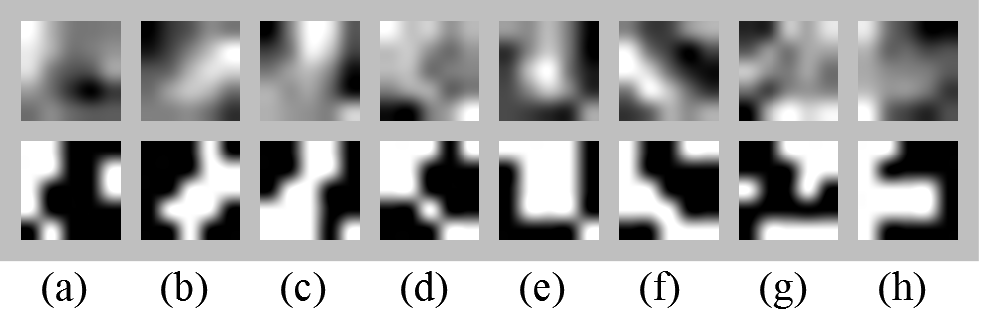
Figure 10: $CK_{8}P_{8}$ filters in the convolutional layer. The first row displays the intensity of the filters’ weights, and the second row indicates whether the weight was positive (white) or negative (black). For visualization, the filters were resized by a factor of twenty using bicubic interpolation and normalized to the range [0,1].

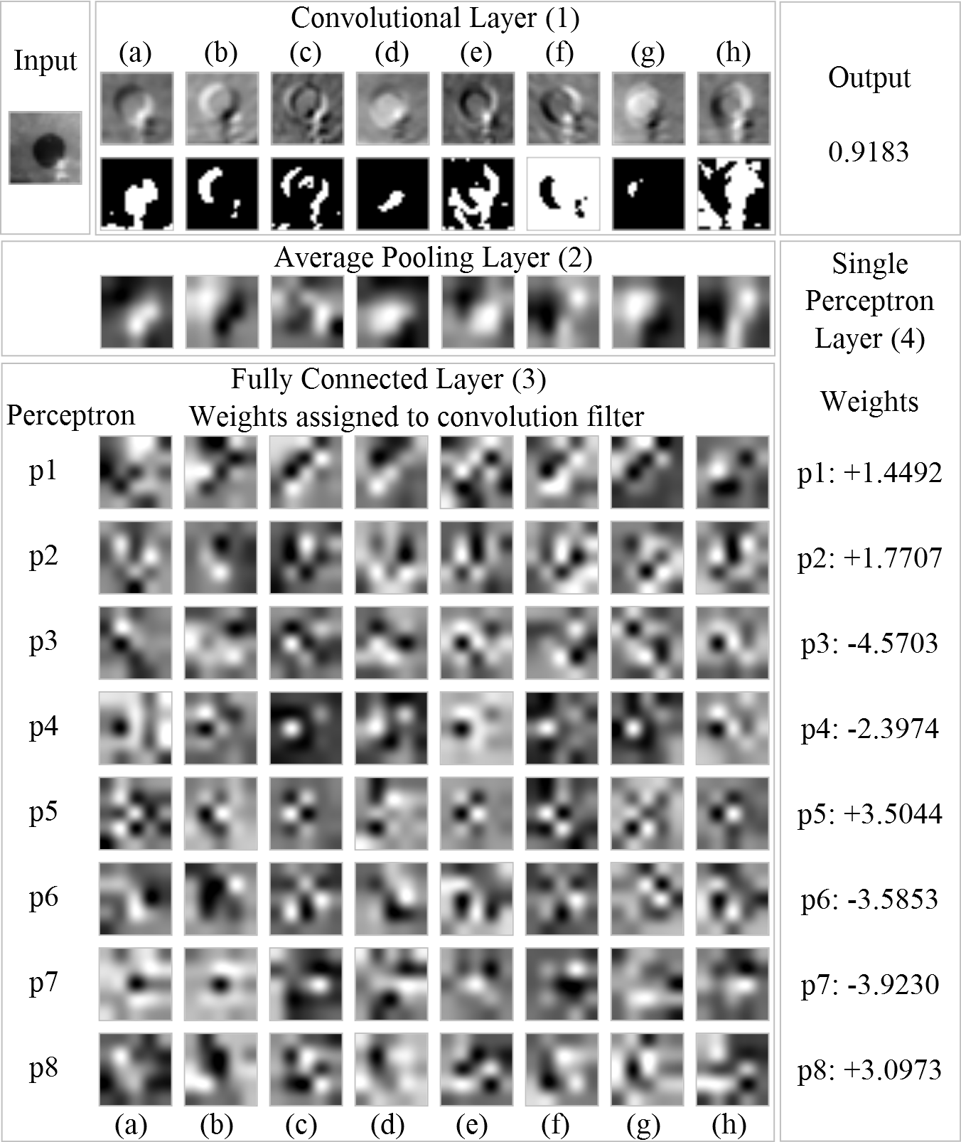
Figure 11: $CK_{8}P_{8}$ response to a valid subregion sample. The convolutional layer includes the filter responses in the first row and positive (in white) and negative (in black) responses in the second row. The fully connected layer shows the weight maps for each perceptron/filter pair. For visualization, the filters were resized by a factor of twenty using bicubic interpolation and normalized to the range [0,1]. The filter order (i.e., (a) to (b) ) matches that of Figure 10.

The weights of all perceptrons in the fully connected layer are also displayed in Figure 11. In the fully connected layer area, the first column identifies the perceptron in the fully connected layer (i.e., from p1 to p8), and the other columns display their respective weights for each of the filters from Figure 10 (i.e., from (a) to (h) ). Since the output weight assigned to perceptrons p1, p2, p5, and p8 are positive, these patterns will respond to centered pupils, while the opposite is true for perceptrons p3, p4, p6, and p7 (see the single perceptron layer in Figure 11). This behavior is caused by the use of a sigmoid function with outputs ranging between zero and one. If a tanh function was used instead, it could lead to negative weights being positive responses. Based on the negative and positive values (Figure 10, second rows of the convolutional layer), the filters (b) and (f) display opposite responses. Based on the input coming from the average pooling layer, p2 displays the best fitting positive weight map for the filter response (a) in the first row of the convolutional layer. Similarly, p1 provides a best fit for (b) and (d), and both p1 and p8 provide good fits for (c) and (f); no perceptron presented an adequate fit for (g) and (h), indicating that these filters are possibly employed to respond to off center pupils. Moreover, all negatively weighted perceptrons present high values at the center for the response filter (e) (the possible center surrounding filter), which could be employed to ignore small blobs. In contrast, p5 (a positively weighted perceptron) weights center responses high.

6 Conclusion

We presented a naturally motivated pipeline of specifically configured CNNs for robust pupil detection and showed that it outperforms state-of-the-art approaches by a large margin while avoiding high computational costs. For the evaluation we used over 79.000 hand labeled images – 41.000 of which were complementary to existing images from the literature – from real-world recordings with artifacts such as reflections, changing illumination conditions, occlusion, etc. Especially for this challenging data set, the CNNs reported considerably higher detection rates than state-of-the-art techniques. Looking forward, we are planning to investigate the applicability of the proposed pipeline to online scenarios, where continuous adaptation of the parameters is a further challenge.

References

- [1] R. A. Boie and I. J. Cox. An analysis of camera noise. IEEE Transactions on Pattern Analysis & Machine Intelligence, 1992.
- [2] D. Ciresan, U. Meier, and J. Schmidhuber. Multi-column deep neural networks for image classification. In Computer Vision and Pattern Recognition (CVPR), 2012 IEEE Conference on, pages 3642–3649. IEEE, 2012.
- [3] L. Cowen, L. J. Ball, and J. Delin. An eye movement analysis of web page usability. In People and Computers XVI-Memorable Yet Invisible, pages 317–335. Springer, 2002.
- [4] P. Domingos. A few useful things to know about machine learning. Communications of the ACM, 55(10):78–87, 2012.
- [5] D. Dussault and P. Hoess. Noise performance comparison of iccd with ccd and emccd cameras. In Optical Science and Technology, the SPIE 49th Annual Meeting, pages 195–204. International Society for Optics and Photonics, 2004.
- [6] M. A. Fischler and R. C. Bolles. Random sample consensus: a paradigm for model fitting with applications to image analysis and automated cartography. Communications of the ACM, 24(6):381–395, 1981.
- [7] W. Fuhl, T. Kübler, K. Sippel, W. Rosenstiel, and E. Kasneci. Excuse: Robust pupil detection in real-world scenarios. In CAIP 16th Inter. Conf. Springer, 2015.
- [8] T. M. Heskes and B. Kappen. On-line learning processes in artificial neural networks. North-Holland Mathematical Library, 51:199–233, 1993.
- [9] Intel Corporation. Intel®Core i7-3500 Mobile Processor Series. Accessed: 2015-11-02.
- [10] A.-H. Javadi, Z. Hakimi, M. Barati, V. Walsh, and L. Tcheang. Set: a pupil detection method using sinusoidal approximation. Frontiers in neuroengineering, 8, 2015.
- [11] E. Kasneci. Towards the automated recognition of assistance need for drivers with impaired visual field. PhD thesis, Universität Tübingen, Germany, 2013.
- [12] E. Kasneci, K. Sippel, K. Aehling, M. Heister, W. Rosenstiel, U. Schiefer, and E. Papageorgiou. Driving with Binocular Visual Field Loss? A Study on a Supervised On-road Parcours with Simultaneous Eye and Head Tracking. Plos One, 9(2):e87470, 2014.
- [13] E. Kasneci, K. Sippel, M. Heister, K. Aehling, W. Rosenstiel, U. Schiefer, and E. Papageorgiou. Homonymous visual field loss and its impact on visual exploration: A supermarket study. TVST, 3, 2014.
- [14] M. Kassner, W. Patera, and A. Bulling. Pupil: an open source platform for pervasive eye tracking and mobile gaze-based interaction. In Proceedings of the 2014 ACM International Joint Conference on Pervasive and Ubiquitous Computing: Adjunct Publication, pages 1151–1160. ACM, 2014.
- [15] A. Keil, G. Albuquerque, K. Berger, and M. A. Magnor. Real-time gaze tracking with a consumer-grade video camera. 2010.
- [16] A. Krizhevsky, I. Sutskever, and G. E. Hinton. Imagenet classification with deep convolutional neural networks. In Advances in neural information processing systems, pages 1097–1105, 2012.
- [17] Y. LeCun, L. Bottou, Y. Bengio, and P. Haffner. Gradient-based learning applied to document recognition. Proceedings of the IEEE, 86(11):2278–2324, 1998.
- [18] Y. A. LeCun, L. Bottou, G. B. Orr, and K.-R. Müller. Efficient backprop. In Neural networks: Tricks of the trade, pages 9–48. Springer, 2012.
- [19] D. Li, D. Winfield, and D. J. Parkhurst. Starburst: A hybrid algorithm for video-based eye tracking combining feature-based and model-based approaches. In CVPR Workshops 2005. IEEE Computer Society Conference on. IEEE, 2005.
- [20] L. Lin, L. Pan, L. Wei, and L. Yu. A robust and accurate detection of pupil images. In BMEI 2010, volume 1. IEEE, 2010.
- [21] X. Liu, F. Xu, and K. Fujimura. Real-time eye detection and tracking for driver observation under various light conditions. In Intelligent Vehicle Symposium, 2002. IEEE, volume 2, 2002.
- [22] X. Long, O. K. Tonguz, and A. Kiderman. A high speed eye tracking system with robust pupil center estimation algorithm. In EMBS 2007. IEEE, 2007.
- [23] G. B. Orr. Dynamics and algorithms for stochastic learning. PhD thesis, PhD thesis, Department of Computer Science and Engineering, Oregon Graduate Institute, Beaverton, OR 97006, 1995. ftp://neural. cse. ogi. edu/pub/neural/papers/orrPhDch1-5. ps. Z, orrPhDch6-9. ps. Z, 1995.
- [24] R. B. Palm. Prediction as a candidate for learning deep hierarchical models of data. Technical University of Denmark, 2012.
- [25] A. Peréz, M. Cordoba, A. Garcia, R. Méndez, M. Munoz, J. L. Pedraza, and F. Sanchez. A precise eye-gaze detection and tracking system. 2003.
- [26] Y. Reibel, M. Jung, M. Bouhifd, B. Cunin, and C. Draman. Ccd or cmos camera noise characterisation. The European Physical Journal Applied Physics, 21(01):75–80, 2003.
- [27] J. San Agustin, H. Skovsgaard, E. Mollenbach, M. Barret, M. Tall, D. W. Hansen, and J. P. Hansen. Evaluation of a low-cost open-source gaze tracker. In Proceedings of the 2010 Symposium on Eye-Tracking Research & Applications, pages 77–80. ACM, 2010.
- [28] S. K. Schnipke and M. W. Todd. Trials and tribulations of using an eye-tracking system. In CHI’00 ext. abstr. ACM, 2000.
- [29] L. Świrski, A. Bulling, and N. Dodgson. Robust real-time pupil tracking in highly off-axis images. In Proceedings of the Symposium on ETRA. ACM, 2012.
- [30] S. Trösterer, A. Meschtscherjakov, D. Wilfinger, and M. Tscheligi. Eye tracking in the car: Challenges in a dual-task scenario on a test track. In Proceedings of the 6th AutomotiveUI. ACM, 2014.
- [31] J. Turner, J. Alexander, A. Bulling, D. Schmidt, and H. Gellersen. Eye pull, eye push: Moving objects between large screens and personal devices with gaze and touch. In Human-Computer Interaction–INTERACT 2013, pages 170–186. Springer, 2013.
- [32] N. Wade and B. W. Tatler. The moving tablet of the eye: The origins of modern eye movement research. Oxford University Press, 2005.
- [33] A. Yarbus. The perception of an image fixed with respect to the retina. Biophysics, 2(1):683–690, 1957.