A Closed-Form Solution to Tensor Voting: Theory and Applications

Abstract

We prove a closed-form solution to tensor voting (CFTV): given a point set in any dimensions, our closed-form solution provides an exact, continuous and efficient algorithm for computing a structure-aware tensor that simultaneously achieves salient structure detection and outlier attenuation. Using CFTV, we prove the convergence of tensor voting on a Markov random field (MRF), thus termed as MRFTV, where the structure-aware tensor at each input site reaches a stationary state upon convergence in structure propagation. We then embed structure-aware tensor into expectation maximization (EM) for optimizing a single linear structure to achieve efficient and robust parameter estimation. Specifically, our EMTV algorithm optimizes both the tensor and fitting parameters and does not require random sampling consensus typically used in existing robust statistical techniques. We performed quantitative evaluation on its accuracy and robustness, showing that EMTV performs better than the original TV and other state-of-the-art techniques in fundamental matrix estimation for multiview stereo matching. The extensions of CFTV and EMTV for extracting multiple and nonlinear structures are underway. An addendum is included in this arXiv version.

Abstract

We respond to the comments paper [1] on the proof to the closed-form solution to tensor voting [2] or CFTV. First, the proof is correct and let ${\mathbf{S}}$ be the resulting tensor which may be asymmetric. Second, ${\mathbf{S}}$ should be interpreted using singular value decomposition (SVD), where the symmetricity of ${\mathbf{S}}$ is unimportant, because the corresponding eigensystems to the positive semidefinite (PSD) systems, namely, ${\mathbf{S}}{\mathbf{S}}^{T}$ or ${\mathbf{S}}^{T}{\mathbf{S}}$, are used in practice. Finally, we prove a symmetric version of CFTV, run extensive simulations and show that the original tensor voting, the asymmetric CFTV and symmetric CFTV produce practically the same empirical results in tensor direction except in high uncertainty situations due to ball tensors and low saliency.

1 Introduction

This paper reinvents tensor voting [19] for robust computer vision, by proving a closed-form solution to computing an exact structure-aware tensor after data communication in a feature space of any dimensions, where the goal is salient structure inference from noisy and corrupted data.

To infer structures from noisy data corrupted by outliers, in tensor voting, input points communicate among themselves subject to proximity and continuity constraints. Consequently, each point is aware of its structure saliency via a structure-aware tensor. Structure refers to surfaces, curves, or junctions if the feature space is three dimensional where a structure-aware tensor can be visualized as an ellipsoid: if a point belongs to a smooth surface, the resulting ellipsoid after data communication resembles a stick pointing along the surface normal; if a point lies on a curve the tensor resembles a plate, where the curve tangent is perpendicular to the plate tensor; if it is a point junction where surfaces intersect, the tensor will be like a ball. An outlier is characterized by a set of inconsistent votes it receives after data communication.

We develop in this paper a closed-form solution to tensor voting (CFTV), which is applicable to the special as well as general theory of tensor voting. This paper focuses on the special theory, where the above data communication is data driven without using constraints other than proximity and continuity. The special theory, sometimes coined as “first voting pass,” is applied to process raw input data to detect structures and outliers. In addition to structure detection and outlier attenuation, in the general theory of tensor voting, tensor votes are propagated along preferred directions to achieve data communication when such directions are available, typically after the first pass, such that useful tensor votes are reinforced whereas irrelevant ones are suppressed.

Figure 1: Inlier/outlier and tensor inverse illustration. (a) The normal votes received at a surface point cast by points in ${\mathbf{x}}$’s neighborhood. Three salient outliers are present. (b) For a non-surface point, there is no preference to any normals. (c) The structure-aware tensor induced by the normal observations in (a), which is represented by a $d$-D ellipsoid, where $d\geq 2$. The orange curve (dashed curve) represents the variance produced along all possible directions. (d) The structure-aware tensor collected after collecting the received votes in (b). (e) and (f) correspond to the inverse of (c) and (d), respectively.

Expressing tensor voting in a single and compact equation, or a closed-form solution, offers many advantages: not only an exact and efficient solution can be achieved with less implementation effort for salient structure detection and outlier attenuation, formal and useful mathematical operations such as differential calculus can be applied which is otherwise impossible using the original tensor voting procedure. Notably, we can prove the convergence of tensor voting on Markov random fields (MRFTV) where a structure-aware tensor at each input site achieves a stationary state upon convergence.

Using CFTV, we contribute a mathematical derivation based on expectation maximization (EM) that applies the exact tensor solution for extracting the most salient linear structure, despite that the input data is highly corrupted. Our algorithm is called EMTV, which optimizes both the tensor and fitting parameters upon convergence and does not require random sampling consensus typical of existing robust statistical techniques. The extension to extract salient multiple and nonlinear structures is underway.

While the mathematical derivation may seem involved, our main results for CFTV, MRFTV and EMTV, that is, Eqns (11), (12), (18), (19), (28), and (6.4). have rigorous mathematical foundations, are applicable to any dimensions, produce more robust and accurate results as demonstrated in our qualitative and quantitative evaluation using challenging synthetic and real data, but on the other hand are easier to implement. The source codes accompanying this paper are available in the supplemental material.

2 Related Work

While this paper is mainly concerned with tensor voting, we provide a concise review on robust estimation and expectation maximization.

Robust estimators. Robust techniques are widely used and an excellent review of the theoretical foundations of robust methods in the context of computer vision can be found in [20].

The Hough transform [13] is a robust voting-based technique operating in a parameter space capable of extracting multiple models from noisy data. Statistical Hough transform [6] can be used for high dimensional spaces with sparse observations. Mean shift [5] has been widely used since its introduction to computer vision for robust feature space analysis. The Adaptive mean shift [11] with variable bandwidth in high dimensions was introduced in texture classification and has since been applied to other vision tasks. Another popular robust method in computer vision is in the class of random sampling consensus (RANSAC) procedures [7] which have spawned a lot of follow-up work (e.g., optimal randomized RANSAC [4]).

Like RANSAC [7], robust estimators including the LMedS [22] and the M-estimator [14] adopted a statistical approach. The LMedS, RANSAC and the Hough transform can be expressed as M-estimators with auxiliary scale [20]. The choice of scales and parameters related to the noise level are major issues. Existing works on robust scale estimation use random sampling [26], or operate on different assumptions (e.g., more than 50% of the data should be inliers [23]; inliers have a Gaussian distribution [15]). Among them, the Adaptive Scale Sample Consensus (ASSC) estimator [28] has shown the best performance where the estimation process requires no free parameter as input. Rather than using a Gaussian distribution to model inliers, the authors of [28] proposed to use a two-step scale estimator (TSSE) to refine the model scale: first, a non-Gaussian distribution is used to model inliers where local peaks of density are found by mean shift [5]; second, the scale parameter is estimated by a median scale estimator with the estimated peaks and valleys. On the other hand, the projection-based M-estimator (pbM) [3], an improvement made on the M-estimator, uses a Parzen window for scale estimation, so the scale parameter is automatically found by searching for the normal direction (projection direction) that maximizes the sharpest peak of the density. This does not require an input scale from the user. While these recent methods can tolerate more outliers, most of them still rely on or are based on RANSAC and a number of random sampling trials is required to achieve the desired robustness.

To reject outliers, a multi-pass method using $L_{\infty}$-norms was proposed to successively detect outliers which are characterized by maximum errors [24].

Expectation Maximization. EM has been used in handling missing data and identifying outliers in robust computer vision [8], and its convergence properties were studied [18]. In essence, EM consists of two steps [2, 18]:

1. E-Step. Computing an expected value for the complete data set using incomplete data and the current estimates of the parameters.

2. M-Step. Maximizing the complete data log-likelihood using the expected value computed in the E-step.

EM is a powerful inference algorithm, but it is also well-known from [8] that: 1) initialization is an issue because EM can get stuck in poor local minima, and 2) treatment of data points with small expected weights requires great care. They should not be regarded as negligible, as their aggregate effect can be quite significant. In this paper we initialize EMTV using structure-aware tensors obtained by CFTV. As we will demonstrate, such initialization not only allows the EMTV algorithm to converge quickly (typically within 20 iterations) but also produces accurate and robust solution in parameter estimation and outlier rejection.

3 Data Communication

In the tensor voting framework, a data point, or voter, communicates with another data point, or vote receiver, subject to proximity and continuity constraints, resulting in a tensor vote cast from the voter to the vote receiver (Fig. 1). In the following, we use $\mathbf{n}$ to denote a unit voting stick tensor, ${\bf v}$ to denote a stick tensor vote received. Stick tensor vote may not be unit vectors when they are multiplied by vote strength. These stick tensors are building elements of a structure-aware tensor vote.

Here, we first define a decay function $\eta$ to encode the proximity and smoothness constraints (Eqns 1 and 2). While similar in effect to the decay function used in the original tensor voting, and also to the one used in [9] where a vote attenuation function is defined to decouple proximity and curvature terms, our modified function, which also differs from that in [21], enables a closed-form solution for tensor voting without resorting to precomputed discrete voting fields.

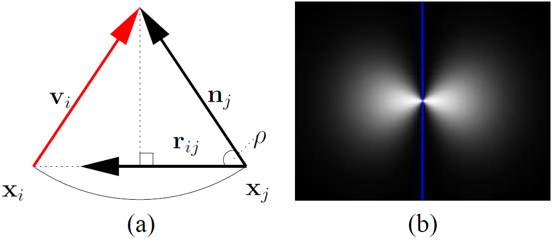
Figure 2: (a) The normal vote ${\mathbf{v}}_{i}$ received at ${\mathbf{x}}_{i}$ using an arc of the osculating circle between ${\mathbf{x}}_{i}$ and ${\mathbf{x}}_{j}$, assuming the normal voter at ${\mathbf{x}}_{j}$ is $\mathbf{n}_{j}$, where $\mathbf{n}_{j}$, ${\mathbf{r}}_{ij}$, and ${\mathbf{v}}_{i}$ are unit vectors in this illustration. (b) Plot of Eqn. (1) in 2D.

Refer to Fig. 2. Consider two points ${\mathbf{x}}_{i}\in\mathbb{R}^{d}$ and ${\mathbf{x}}_{j}\in\mathbb{R}^{d}$ (where $d>1$ is the dimension) that are connected by some smooth structure in the feature/solution space. Suppose that the unit normal $\mathbf{n}_{j}$ at ${\mathbf{x}}_{j}$ is known. We want to generate at ${\mathbf{x}}_{i}$ a normal (vote) ${\mathbf{v}}_{i}$ so that we can calculate $\mathbf{K}_{i}\in\mathbb{R}^{d}\times\mathbb{R}^{d}$, where $\mathbf{K}_{i}$ is the structure-aware tensor at ${\mathbf{x}}_{i}$ in the presence of ${\mathbf{n}}_{j}$ at ${\mathbf{x}}_{j}$. In tensor voting, a structure-aware tensor is a second-order symmetric tensor which can be visualized as an ellipsoid.

While many possibilities exist, the unit direction ${\mathbf{v}}_{i}$ can be derived by fitting an arc of the osculating circle between the two points. Such an arc keeps the curvature constant along the hypothesized connection, thus encoding the smoothness constraint. $\mathbf{K}_{i}$ is then given by ${\mathbf{v}}_{i}{\mathbf{v}}_{i}^{T}$ multiplied by $\eta({\mathbf{x}}_{i},{\mathbf{x}}_{j},\mathbf{n}_{j})$ defined as:

$$\eta({\mathbf{x}}_{i},{\mathbf{x}}_{j},\mathbf{n}_{j})=c_{ij}(1-(\mathbf{r}_{ij}^{T}\mathbf{n}_{j})^{2})$$ (1)

where

$$c_{ij}=\exp(-\frac{||{\mathbf{x}}_{i}-{\mathbf{x}}_{j}||^{2}}{\sigma_{d}})$$ (2)

is an exponential function using Euclidean distance for attenuating the strength based on proximity. $\sigma_{d}$ is the size of local neighborhood (or the scale parameter, the only free parameter in tensor voting).

In Eqn. (1), ${\mathbf{r}}_{ij}\in\mathbb{R}^{d}$ is a unit vector at ${\mathbf{x}}_{j}$ pointing to ${\mathbf{x}}_{i}$, and $1-({\mathbf{r}}_{ij}^{T}\mathbf{n}_{j})^{2}$ is a squared-sine function for attenuating the contribution according to curvature. Similar to the original tensor voting framework, Eqn. (1) favors nearby neighbors that produce small-curvature connections, thus encoding the smoothness constraint. A plot of the 2D version of Eqn. (1) is shown in Fig. 2(b), where ${\mathbf{x}}_{j}$ is located at the center of the image and ${\mathbf{n}}_{j}$ is aligned with the blue line. The higher the intensity, the higher the value Eqn. (1) produces at a given pixel location.

Next, consider the general case where the normal $\mathbf{n}_{j}$ at ${\mathbf{x}}_{j}$ is unavailable. Here, let ${\mathbf{K}}_{j}$ at ${\mathbf{x}}_{j}$ be any second-order symmetric tensor, which is typically initialized as an identity matrix if no normal information is available.

To compute $\mathbf{K}_{i}$ given ${\mathbf{K}}_{j}$, we consider equivalently the set of all possible unit normals $\{\mathbf{n}_{\theta j}\}$ associated with the corresponding length $\{\tau_{\theta j}\}$ which make up ${\mathbf{K}}_{j}$ at ${\mathbf{x}}_{j}$, where $\{\mathbf{n}_{\theta j}\}$ and $\{\tau_{\theta j}\}$ are respectively indexed by all possible directions $\theta$. Each $\tau_{\theta j}\mathbf{n}_{\theta j}$ postulates a normal vote ${\bf v}_{\theta}({\mathbf{x}}_{i},{\mathbf{x}}_{j})$ at ${\mathbf{x}}_{i}$ under the same smoothness constraint prescribed by the corresponding arc of the osculating circle as illustrated in Fig. 3.

Let ${\mathbf{S}}_{ij}$ be the second-order symmetric tensor vote obtained at ${\mathbf{x}}_{i}$ due to this complete set of normals at ${\mathbf{x}}_{j}$ defined above. We have

$${\mathbf{S}}_{ij}=\int_{\mathbf{N}_{\theta j}\in\nu}{\bf v}_{\theta}({\mathbf{x}}_{i},{\mathbf{x}}_{j}){\bf v}_{\theta}({\mathbf{x}}_{i},{\mathbf{x}}_{j})^{T}\eta({\mathbf{x}}_{i},{\mathbf{x}}_{j},\mathbf{n}_{\theta j})d\mathbf{N}_{\theta j}$$ (3)

where

$$\mathbf{N}_{\theta j}=\mathbf{n}_{\theta j}\mathbf{n}_{\theta j}^{T}$$ (4)

and $\nu$ is the space containing all possible $\mathbf{N}_{\theta j}$. For example, if $\nu$ is 2D, the complete set of unit normals $\mathbf{n}_{\theta}$ describes a unit circle. If $\nu$ is 3D, the complete set of unit normals $\mathbf{n}_{\theta}$ describes a unit sphere.

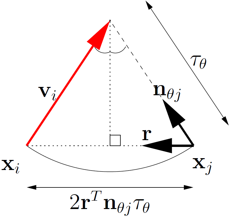
Figure 3: Illustration of Eqn. (5). Normal vote ${\mathbf{v}}_{i}={\mathbf{v}}_{\theta}({\mathbf{x}}_{i},{\mathbf{x}}_{j})$ received at ${\mathbf{x}}_{i}$ using the arc of the osculating circle between ${\mathbf{x}}_{i}$ and ${\mathbf{x}}_{j}$, considering one of the normal voters at ${\mathbf{x}}_{j}$ is $\mathbf{n}_{\theta j}$. Here, $\mathbf{n}_{\theta j}$ and ${\mathbf{r}}$ are unit vectors.

In a typical tensor voting implementation, Eqn. (3) is precomputed as discrete voting fields (e.g., plate and ball voting fields in 3D tensor voting [19]): the integration is implemented by rotating and summing the contributions using matrix addition. Although precomputed once, such discrete approximations involve uniform and dense sampling of tensor votes $\mathbf{n}_{\theta}\mathbf{n}_{\theta}^{T}$ in higher dimensions where the number of dimensions depends on the problem. In the following section, we will prove a closed-form solution to Eqn. (3), which provides an efficient and exact solution to computing ${\mathbf{K}}$ without resorting to discrete and dense sampling.

Figure 4: (a) 3D ball voting field. A slice generated using the closed-form solution Eqn (11), which has similar tensor orientations (but different tensor strengths) as the ball voting field in [19]. (b) 3D plate voting field. Left: a cut of the voting field (direction of $\hat{e}_{3}$ normal to the page). Right: a cut of the same voting field, showing the $(\lambda_{2}-\lambda_{3})\hat{e}_{3}$ component (i.e., component parallel to the tangent direction). The field is generated by using Eqn (11) showing similar tensor orientations as the plate voting field in [19]. (c) 3D stick voting field. A slice after zeroing out votes lying in the 45-degree zone as done in [19]. The stick tensor orientations shown in the figure are identical to those in the 3D stick voting field in [19]. (d) Vote computation using the closed-form solution in one single step by Eqn (11).

4 Closed-Form Solution

Theorem 1

(Closed-Form Solution to Tensor Voting) The tensor vote at ${\mathbf{x}}_{i}$ induced by ${\mathbf{K}}_{j}$ located at ${\mathbf{x}}_{j}$ is given by the following closed-form solution:

$${\mathbf{S}}_{ij}=c_{ij}{\mathbf{R}}_{ij}{\mathbf{K}}_{j}{\mathbf{R}}^{\prime}_{ij}$$

where ${\mathbf{K}}_{j}$ is a second-order symmetric tensor, ${\mathbf{R}}_{ij}={\mathbf{I}}-2{\mathbf{r}}_{ij}{\mathbf{r}}_{ij}^{T}$, ${\mathbf{R}}^{\prime}_{ij}=({\mathbf{I}}-\frac{1}{2}{\mathbf{r}}_{ij}{\mathbf{r}}_{ij}^{T}){\mathbf{R}}_{ij}$, ${\mathbf{I}}$ is an identity, ${\mathbf{r}}_{ij}$ is a unit vector pointing from ${\mathbf{x}}_{j}$ to ${\mathbf{x}}_{i}$ and $c_{ij}=\exp(-\frac{||{\mathbf{x}}_{i}-{\mathbf{x}}_{j}||^{2}}{\sigma_{d}})$ with $\sigma_{d}$ as the scale parameter.

Proof 2

For simplicity of notation, set ${\mathbf{r}}={\mathbf{r}}_{ij}$, $\mathbf{n}_{\theta}=\mathbf{n}_{\theta j}$ and ${\mathbf{N}}_{\theta}={\mathbf{N}}_{\theta j}$. Now, using the above-mentioned osculating arc connection, ${\bf v}_{\theta}({\mathbf{x}}_{i},{\mathbf{x}}_{j})$ can be expressed as

$${\bf v}_{\theta}({\mathbf{x}}_{i},{\mathbf{x}}_{j})=(\mathbf{n}_{\theta}-2\mathbf{r}(\mathbf{r}^{T}\mathbf{n}_{\theta}))\tau_{\theta}$$ (5)

Recall that $\mathbf{n}_{\theta}$ is the unit normal at ${\mathbf{x}}_{j}$ with direction $\theta$, and that $\tau_{\theta}$ is the length associated with the normal. This vector subtraction equation is shown in Fig. 3 where the roles of ${\bf v}_{\theta},\mathbf{n}_{\theta},\mathbf{r}$, and $\tau_{\theta}$ are illustrated.

Let

$$\mathbf{R}=(\mathbf{I}-2\mathbf{r}\mathbf{r}^{T}),$$ (6)

where $\mathbf{I}$ is an identity, we can rewrite Eqn. (3) into the following form:

$${\mathbf{S}}_{ij}=c_{ij}\int_{\mathbf{N}_{\theta}\in\nu}\tau_{\theta}^{2}\mathbf{R}\mathbf{n}_{\theta}\mathbf{n}_{\theta}^{T}\mathbf{R}^{T}(1-(\mathbf{n}_{\theta}^{T}\mathbf{r})^{2})d\mathbf{N}_{\theta}.$$ (7)

Following the derivation:

$${\mathbf{S}}_{ij} = c_{ij}\int_{\mathbf{N}_{\theta}\in\nu}\tau_{\theta}^{2}\mathbf{R}\mathbf{n}_{\theta}(1-(\mathbf{n}_{\theta}^{T}\mathbf{r})^{2})\mathbf{n}_{\theta}^{T}\mathbf{R}^{T}d\mathbf{N}_{\theta}$$ (8)

$$= c_{ij}\mathbf{R}\left(\int_{\mathbf{N}_{\theta}\in\nu}\tau_{\theta}^{2}\mathbf{n}_{\theta}(1-\mathbf{n}_{\theta}^{T}\mathbf{r}\mathbf{r}^{T}\mathbf{n}_{\theta})\mathbf{n}_{\theta}^{T}d\mathbf{N}_{\theta}\right)\mathbf{R}^{T}$$

$$= c_{ij}\mathbf{R}\left(\int_{\mathbf{N}_{\theta}\in\nu}\tau_{\theta}^{2}\mathbf{N}_{\theta}-\tau_{\theta}^{2}\mathbf{N}_{\theta}\mathbf{r}\mathbf{r}^{T}\mathbf{N}_{\theta}d\mathbf{N}_{\theta}\right)\mathbf{R}^{T}$$

$$= c_{ij}\mathbf{R}\left(\mathbf{K}_{j}-\int_{\mathbf{N}_{\theta}\in\nu}\tau_{\theta}^{2}\mathbf{N}_{\theta}\mathbf{r}\mathbf{r}^{T}\mathbf{N}_{\theta}d\mathbf{N}_{\theta}\right)\mathbf{R}^{T}$$

The integration can be solved by integration by parts. Let $f(\theta)=\tau_{\theta}^{2}\mathbf{N}_{\theta}$, $f^{\prime}(\theta)=\tau_{\theta}^{2}\mathbf{I}$, $g(\theta)=\frac{1}{2}\mathbf{r}\mathbf{r}^{T}\mathbf{N}_{\theta}^{2}$ and $g^{\prime}(\theta)=\mathbf{r}\mathbf{r}^{T}\mathbf{N}_{\theta}$, and note that $\mathbf{N}_{\theta}^{q}=\mathbf{N}_{\theta}$ for all $q\in\mathbb{Z}^{+}$ (see this footnote), and ${\mathbf{K}}_{j}$, in the most general form, can be expressed as a generic tensor $\int_{\mathbf{N}_{\theta}\in\nu}\tau_{\theta}^{2}\mathbf{N}_{\theta}d\mathbf{N}_{\theta}$. So we have

$$\int_{\mathbf{N}_{\theta}\in\nu}\tau_{\theta}^{2}\mathbf{N}_{\theta}\mathbf{r}\mathbf{r}^{T}\mathbf{N}_{\theta}d\mathbf{N}_{\theta}$$

$$= \left[f(\theta)g(\theta)\right]_{\mathbf{N}_{\theta}\in\nu}-\int_{\mathbf{N}_{\theta}\in\nu}f^{\prime}(\theta)g(\theta)d\mathbf{N}_{\theta}$$

$$= \left[\frac{1}{2}\tau_{\theta}^{2}\mathbf{N}_{\theta}\mathbf{r}\mathbf{r}^{T}\mathbf{N}_{\theta}^{2}\right]_{\mathbf{N}_{\theta}\in\nu}-\frac{1}{2}\int_{\mathbf{N}_{\theta}\in\nu}\tau_{\theta}^{2}\mathbf{r}\mathbf{r}^{T}\mathbf{N}_{\theta}d\mathbf{N}_{\theta}$$

$$= \frac{1}{2}\int_{{\mathbf{N}}_{\theta}\in\nu}\left(\tau_{\theta}^{2}\frac{d}{d{\mathbf{N}}_{\theta}}[{\mathbf{N}}_{\theta}]{\mathbf{r}}{\mathbf{r}}^{T}{\mathbf{N}}_{\theta}^{2}+\tau_{\theta}^{2}{\mathbf{N}}_{\theta}\frac{d}{d{\mathbf{N}}_{\theta}}[{\mathbf{r}}{\mathbf{r}}^{T}{\mathbf{N}}_{\theta}^{2}]\right)d{\mathbf{N}}_{\theta}$$

$$-\frac{1}{2}{\mathbf{r}}{\mathbf{r}}^{T}{\mathbf{K}}_{j}.$$

The explanation for the last equality above is given in this footnote.

Finally, we apply the fact that $\mathbf{N}_{\theta}^{q}=\mathbf{N}_{\theta}$ (for all $q\in\mathbb{Z}^{+}$) to convert $\frac{d}{d{\mathbf{N}}_{\theta}}[{\mathbf{r}}{\mathbf{r}}^{T}{\mathbf{N}}_{\theta}^{2}]$ into $\frac{d}{d{\mathbf{N}}_{\theta}}[{\mathbf{r}}{\mathbf{r}}^{T}{\mathbf{N}}_{\theta}]$. We obtain

$$\frac{1}{2}\int_{{\mathbf{N}}_{\theta}\in\nu}\left(\tau_{\theta}^{2}{\mathbf{r}}{\mathbf{r}}^{T}{\mathbf{N}}_{\theta}^{2}+\tau_{\theta}^{2}{\mathbf{N}}_{\theta}{\mathbf{r}}{\mathbf{r}}^{T}\right)d{\mathbf{N}}_{\theta}-\frac{1}{2}{\mathbf{r}}{\mathbf{r}}^{T}{\mathbf{K}}_{j}$$ (9)

$$= \frac{1}{2}\left({\mathbf{r}}{\mathbf{r}}^{T}{\mathbf{K}}_{j}+{\mathbf{K}}_{j}{\mathbf{r}}{\mathbf{r}}^{T}-{\mathbf{r}}{\mathbf{r}}^{T}{\mathbf{K}}_{j}\right)$$

$$= \frac{1}{2}{\mathbf{K}}_{j}\mathbf{r}\mathbf{r}^{T}.$$

By substituting Eqn. (9) back to Eqn. (37), we obtain the result as follows:

$${\mathbf{S}}_{ij}=c_{ij}{\mathbf{R}}{\mathbf{K}}_{j}\left(\mathbf{I}-\frac{1}{2}\mathbf{r}\mathbf{r}^{T}\right){\mathbf{R}}^{T}.\\$$ (10)

Replace $\mathbf{r}$ by ${\mathbf{r}}_{ij}$ such that ${\mathbf{R}}_{ij}={\mathbf{I}}-2{\mathbf{r}}_{ij}{\mathbf{r}}_{ij}^{T}$ and let ${\mathbf{R}}^{\prime}_{ij}=({\mathbf{I}}-\frac{1}{2}{\mathbf{r}}_{ij}{\mathbf{r}}_{ij}^{T}){\mathbf{R}}_{ij}$, we obtain

$${\mathbf{S}}_{ij}=c_{ij}{\mathbf{R}}_{ij}{\mathbf{K}}_{j}{\mathbf{R}}^{\prime}_{ij}.$$ (11)

A structure-aware tensor ${\mathbf{K}}_{i}=\sum_{j}{\mathbf{S}}_{ij}$ can thus be assigned at each site ${\mathbf{x}}_{i}$. This tensor sum considers both geometric proximity and smoothness constraints in the presence of neighbors ${\mathbf{x}}_{j}$ under the chosen scale of analysis. Note also that Eqn. (11) is an exact equivalent of Eqn. (3), or (7), that is, the first principle. Since the first principle produces a positive semi-definite matrix, Eqn. (11) still produces a positive semi-definite matrix.

In tensor voting, eigen-decomposition is applied to a structure-aware tensor. In three dimensions, the eigensystem has eigenvalues $\lambda_{1}\geq\lambda_{2}\geq\lambda_{3}\geq 0$ with the corresponding eigenvectors $\hat{e}_{1},\hat{e}_{2}$, and $\hat{e}_{3}$. $\lambda_{1}-\lambda_{2}$ denotes surface saliency with normal direction indicated by $\hat{e}_{1}$; $\lambda_{2}-\lambda_{3}$ denotes curve saliency with tangent direction indicated by $\hat{e}_{3}$; junction saliency is indicated by $\lambda_{3}$.

While it may be difficult to observe any geometric intuition directly from this closed-form solution, the geometric meaning of the closed-form solution has been described by Eqn. (3) (or (7), the first principle), since Eqn. (11) is equivalent to Eqn. (3). Note that our solution is different from, for instance, [21], where the $N$-D formulation is approached from a more geometric point of view.

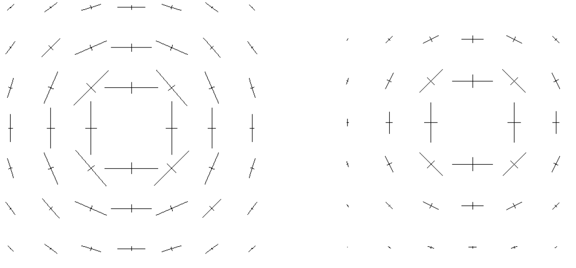
Figure 5: Close-ups of ball voting fields generated using the original tensor voting framework (left) and CFTV (right).

As will be shown in the next section on EMTV, the inverse of ${\mathbf{K}}_{j}$ is used. In case of a perfect stick tensor, which can be equivalently represented as a rank-1 matrix, does not have an inverse. Similar in spirit where a Gaussian function can be interpreted as an impulse function associated with a spread representing uncertainty, a similar statistical approach is adopted here in characterizing our tensor inverse. Specifically, the uncertainty is incorporated using a ball tensor, where $\epsilon{\mathbf{I}}$ is added to ${\mathbf{K}}_{j}$, $\epsilon$ is a small positive constant (0.001) and ${\mathbf{I}}$ an identity matrix. Fig. 1 shows a tensor and its inverse for some selected cases. The following corollary regarding the inverse of ${\mathbf{S}}_{ij}$ is useful:

Corollary 1

Let ${\mathbf{R}}{{}^{\prime\prime}}_{ij}={\mathbf{R}}_{ij}({\mathbf{I}}+{\mathbf{r}}_{ij}{\mathbf{r}}_{ij}^{T})$ and also note that ${\mathbf{R}}_{ij}^{-1}={\mathbf{R}}_{ij}$, the corresponding inverse of ${\mathbf{S}}_{ij}$ is:

$${\mathbf{S}}_{ij}^{\prime}=c_{ij}^{-1}{\mathbf{R}}{{}^{\prime\prime}}_{ij}{\mathbf{K}}_{j}^{-1}{\mathbf{R}}_{ij}$$ (12)

Proof 3

This corollary can simply be proved by applying inverse to Eqn (11).

Note the initial ${\mathbf{K}}_{j}$ can be either derived when input direction is available, or simply assigned as an identity matrix otherwise.

4.1 Examples

Using Eqn (11), given any input ${\mathbf{K}}_{j}$ at site $j$ which is a second-order symmetric tensor, the output tensor ${\mathbf{S}}_{ij}$ can be computed directly. Note that ${\mathbf{R}}_{ij}$ is a $d\times d$ matrix of the same dimensionality $d$ as ${\mathbf{K}}_{j}$. To verify our closed-form solution, we perform the following to compare with the voting fields used by the original tensor voting framework (Fig. 4):

• Set ${\mathbf{K}}$ to be an identity (ball tensor) in Eqn (11) and compute all votes ${\mathbf{S}}$ in a neighhorhood. This procedure generates the ball voting field, Fig. 4(a).

• Set ${\mathbf{K}}$ to be a plate tensor $\left[\begin{array}[]{ccc}1&0&0\\ 0&1&0\\ 0&0&0\end{array}\right]$ in Eqn (11) and compute all votes ${\mathbf{S}}$ in a neighborhood. This procedure generates the plate voting field, Fig. 4(b).

• Set ${\mathbf{K}}$ to be a stick tensor $\left[\begin{array}[]{ccc}1&0&0\\ 0&0&0\\ 0&0&0\end{array}\right]$ in Eqn (11) and compute all votes ${\mathbf{S}}$ in a neighborhood. This procedure generates the stick voting field, Fig. 4(c).

• Set ${\mathbf{K}}$ to be any generic second-order tensor in Eqn (11) to compute a tensor vote ${\mathbf{S}}$ at a given site. We do not need a voting field, or the somewhat complex procedure described in [21]. In one single step using the closed-form solution Eqn (11), we obtain ${\mathbf{S}}$ as shown in Fig. 4(d).

Note that the stick voting field generation is the same as the closed-form solution given by the arc of an osculating circle. On the other hand, since the closed-form solution does not remove votes lying beyond the 45-degree zone as done in the original framework, it is useful to compare the ball voting field generated using the CFTV and the original framework. Fig. 5 shows the close-ups of the ball voting fields generated using the original framework and CFTV. As anticipated, the tensor orientations are almost the same (with the maximum angular deviation at $4.531^{\circ}$), while the tensor strength is different due to the use of different decay functions. The new computation results in perfect vote orientations which are radial, and the angular discrepancies are due to the discrete approximations in the original solution.

While the above illustrates the usage of Eqn (11) in three dimensions, the equation applies to any dimensions $d$. All of the ${\mathbf{S}}$’s returned by Eqn (11) are second-order symmetric tensors and can be decomposed using eigen-decomposition. The implementation of Eqn (11) is a matter of a few lines of C++ code.

Our “voting without voting fields” method is uniform to any input tensors ${\mathbf{K}}_{j}$ that are second-order symmetric tensor in its closed-form expressed by Eqn (11), where formal mathematical operation can be applied on this compact equation, which is otherwise difficult on the algorithmic procedure described in previous tensor voting papers. Notably, using the closed-form solution, we are now able to prove mathematically the convergence of tensor voting in the next section.

4.2 Time Complexity

Akin to the original tensor voting formalism, each site (input or non-input) communicates with each other on an Markov random field (MRF) in a broad sense, where the number of edges depends on the scale of analysis, parameterized by $\sigma_{d}$ in Eqn (2). In our implementation, we use an efficient data structure such as ANN tree [1] to access a constant number of neighbors ${\mathbf{x}}_{j}$ of each ${\mathbf{x}}_{i}$. It should be noted that under a large scale of analysis where the number of neighbors is sufficiently large, similar number of neighbors are accessed in ours and the original tensor voting implementation.

The speed of accessing nearest neighbors can be greatly increased (polylogarithmic) by using ANN thus making efficient the computation of a structure-aware tensor. Note that the running time for this implementation of closed-from solution is $O(d^{3})$, while the running time for the original tensor voting (TV) is $O(u^{d-1})$, where $d$ is the dimension of the space and $u$ is the number of sampling directions for a given dimension. Because of this, a typical TV implementation precomputes and stores the dense tensor fields. For example, when $d=3$ and $u=180$ for high accuracy, our method requires 27 operation units, while a typical TV implementation requires 32400 operation units. Given 1980 points and the same number of neighbors, the time to compute a structure-aware tensor using our method is about $0.0001$ second; it takes about $0.1$ second for a typical TV implementation to output the corresponding tensor. The measurement was performed on a computer running on a core duo 2GHz CPU with 2GB RAM.

Note that the asymptotic running time for the improved TV in [21] is $O(d\gamma^{2})$ since it applies Gramm-Schmidt process to perform component decomposition, where $\gamma$ is the number of linearly independent set of the tensors. In most of the cases, $\gamma=d$. So, the running time for our method is comparable to [21]. However, their approach does not have a precise mathematical solution.

5 MRFTV

We have proved CFTV for the special theory of tensor voting, or the “first voting pass” for structure inference. Conventionally, tensor voting was done in two passes, where the second pass was used for structure propagation in the preferred direction after disabling the ball component in the structure-aware tensor. What happens if more tensor voting passes are applied? This has never been answered properly.

In this section we provide a convergence proof for tensor voting based on CFTV: the structure-aware tensor obtained at each site achieves a stationary state upon convergence. Our convergence proof makes use of Markov random fields (MRF), thus termed as MRFTV.

It should be noted that the original tensor voting formulation is also constructed on an MRF according to the broad definition, since random variables (that is, the tensors after voting) are defined on the nodes of an undirected graph in which each node is connected to all neighbors within a fixed distance. On the other hand, without CFTV, it was previously difficult to write down an objective function and to prove the convergence. One caveat to note in the following is that we do not disable the ball component in each iteration, which will be addressed in the future in developing the general theory of tensor voting in structure propagation. As we will demonstrate, MRFTV does not smooth out important features (Fig. 6) and still possesses high outlier rejection ability (Fig. 13).

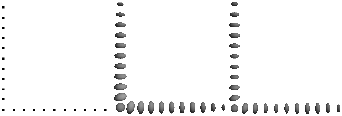
Figure 6: Convergence of MRF-TV. From left to right: input points, result after 2 passes, result after convergence (10 iterations). Visually, this simple example distinguishes tensor voting from smoothing as the sharp orientation discontinuity is preserved upon convergence.

Recall in MRF, a Markov network is a graph consisting of two types of nodes – a set of hidden variables ${\mathbf{E}}$ and a set of observed variables ${\mathbf{O}}$, where the edges of the graph are described by the following posterior probability $\text{P}({\mathbf{E}}|{\mathbf{O}})$ with standard Bayesian framework:

$$\text{P}({\mathbf{E}}|{\mathbf{O}})\propto\text{P}({\mathbf{O}}|{\mathbf{E}})\text{P}({\mathbf{E}})$$ (13)

By letting ${\mathbf{E}}=\{{\mathbf{K}}_{i}|i=1,2,\cdots,N\}$ and ${\mathbf{O}}=\{\tilde{{\mathbf{K}}}_{i}|i=1,2,\cdots,N\}$, where $N$ is total number of points and $\tilde{{\mathbf{K}}}_{i}$ is the known tensor at ${\mathbf{x}}_{i}$, and suppose that inliers follow Gaussian distribution, we obtain the likelihood $\text{P}({\mathbf{O}}|{\mathbf{E}})$ and the prior $\text{P}({\mathbf{E}})$ as follows:

$$\text{P}({\mathbf{O}}|{\mathbf{E}}) \propto \prod_{i}\text{p}(\tilde{{\mathbf{K}}}_{i}|{\mathbf{K}}_{i})=\prod_{i}e^{-\frac{||{\mathbf{K}}_{i}-\tilde{{\mathbf{K}}}_{i}||_{F}^{2}}{\sigma_{h}}}$$ (14)

$$\text{P}({\mathbf{E}}) \propto \prod_{i}\prod_{j\in{\cal N}(i)}\text{p}({\mathbf{S}}_{ij}|{\mathbf{K}}_{i})$$ (15)

$$= \prod_{i}\prod_{j\in{\cal N}(i)}e^{-\frac{||{\mathbf{K}}_{i}-{\mathbf{S}}_{ij}||_{F}^{2}}{\sigma_{s}}}$$ (16)

where $||\cdot||_{F}$ is the Frobenius norm, $\tilde{{\mathbf{K}}}_{i}$ is the known tensor at ${\mathbf{x}}_{i}$, ${\cal N}(i)$ is the set of neighbor corresponds to ${\mathbf{x}}_{i}$ and $\sigma_{h}$ and $\sigma_{s}$ are two constants respectively.

Note that we use the Frobenius norm to encode tensor orientation consistency as well as to reflect the necessary vote saliency information including distance and continuity attenuation. For example, suppose we have a unit stick tensor at ${\mathbf{x}}_{i}$ and a stick vote (received at ${\mathbf{x}}_{i}$), which is parallel to it but with magnitude equal to 0.8. In another scenario ${\mathbf{x}}_{i}$ receives from a voter farther away a stick vote with the same orientation but magnitude being equal to 0.2. The Frobenius norm reflects the difference in saliency despite the perfect orientation consistency in both cases. Notwithstanding, it is arguable that Frobenius norm may not be the perfect solution to encode orientation consistency constraint in the pertinent equations, while this current form works acceptably well in our experiments in practice.

By taking the logarithm of Eqn (13), we obtain the following energy function:

$$E({\mathbf{E}})=\sum_{i}||{\mathbf{K}}_{i}-\tilde{{\mathbf{K}}}_{i}||_{F}^{2}+g\sum_{i}\sum_{j\in{\cal N}(i)}||{\mathbf{K}}_{i}-{\mathbf{S}}_{ij}||_{F}^{2}$$ (17)

where $g=\frac{\sigma_{h}}{\sigma_{s}}$. Theoretically, this quadratic energy function can be directly solved by Singular Value Decomposition (SVD). Since $N$ can be large thus making direct SVD impractical, we adopt an iterative approach: by taking the partial derivative of Eqn (17) (w.r.t. to ${\mathbf{K}}_{i}$) the following update rule is obtained:

$${\mathbf{K}}_{i}^{*}=(\tilde{{\mathbf{K}}}_{i}+2g\sum_{j\in{\cal N}(i)}{\mathbf{S}}_{ij})({\mathbf{I}}+g\sum_{j\in{\cal N}(i)}({\mathbf{I}}+c_{ij}^{2}{{\mathbf{R}}_{ij}^{\prime}}^{2}))^{-1}$$ (18)

which is a Gauss-Seidel solution. When successive over-relaxation (SOR) is employed, the update rule becomes:

$${\mathbf{K}}_{i}^{(m+1)}=(1-q){\mathbf{K}}_{i}^{(m)}+q{\mathbf{K}}_{i}^{*}$$ (19)

where $1<q<2$ is the SOR weight and $m$ is the iteration number. After each iteration, we normalize ${\mathbf{K}}_{i}$ such that the eigenvalues of the corresponding eigensystem are within the range $(0,1]$.

The above proof on convergence of MRF-TV shows that structure-aware tensors achieve stationary states after a finite number Gauss-Seidel iterations in the above formulation. It also dispels a common pitfall that tensor voting is similar in effect to smoothing. Using the same scale of analysis (that is, in (2)) and same $\sigma_{h}$, $\sigma_{s}$ in each iteration, tensor saliency and orientation will both converge. We observe that the converged tensor orientation is in fact similar to that obtained after two voting passes using the original framework, where the orientations at curve junctions are not smoothed out. See Fig. 6 for an example where sharp orientation discontinuity is not smoothed out when tensor voting converges. Here, $\lambda_{1}$ of each structure-aware tensor is not normalized to 1 for visualizing its structure saliency after convergence. Table I summarizes the quantitative comparison with the ground-truth orientation.

TABLE I: Comparison with ground truth for the example in Fig. 6.

6 EMTV

Previously, while tensor voting was capable of rejecting outliers, it fell short of producing accurate parameter estimation, explaining the use of RANSAC in the final parameter estimation step after outlier rejection [27].

This section describes the EMTV algorithm for optimizing a) the structure-aware tensor ${\mathbf{K}}$ at each input site, and b) the parameters of a single plane ${\mathbf{h}}$ of any dimensionality containing the inliers. This algorithm will be applied to stereo matching.

We first formulate the three constraints to be used in EMTV. These constraints are not mutually exclusive, where knowing the values satisfying one constraint will help computing the values of the others. However, in our case, they are all unknowns, so EM is particularly suitable for their optimization, since the expectation calculation and parameter estimation are solved alternately.

6.1 Constraints

Data constraint Suppose we have a set of clean data. One necessary objective is to minimize the following for all ${\mathbf{x}}_{i}\in\mathbb{R}^{d}$ with $d>1$:

$$||{\mathbf{x}}_{i}^{T}{\mathbf{h}}||$$ (20)

where ${\mathbf{h}}\in\mathbb{R}^{d}$ is a unit vector representing the plane (or the model) to be estimated. This is a typical data term that measures the faithfulness of the input data to the fitting plane.

Orientation consistency The plane being estimated is defined by the vector ${\mathbf{h}}$. Since the tensor ${\mathbf{K}}_{i}\in\mathbb{R}^{d}\times\mathbb{R}^{d}$ encodes structure awareness, if ${\mathbf{x}}_{i}$ is an inlier, the orientation information encoded by ${\mathbf{K}}_{i}$ and ${\mathbf{h}}$ have to be consistent. That is, the variance ${\mathbf{h}}^{T}{\mathbf{K}}_{i}^{-1}{\mathbf{h}}$ produced by ${\mathbf{h}}$ should be minimal. Otherwise, ${\mathbf{x}}_{i}$ might be generated by other models even if it minimizes Eqn (20). Mathematically, we minimize:

$$||{\mathbf{h}}^{T}{\mathbf{K}}_{i}^{-1}{\mathbf{h}}||.$$ (21)

Neighborhood consistency While the estimated ${\mathbf{K}}_{i}$ helps to indicate inlier/outlier information, ${\mathbf{K}}_{i}$ has to be consistent with the local structure imposed by its neighbors (when they are known). If ${\mathbf{K}}_{i}$ is consistent with ${\mathbf{h}}$ but not the local neighborhood, either ${\mathbf{h}}$ or ${\mathbf{K}}_{i}$ is wrong. In practice, we minimize the following Frobenius norm as in Eqns (14)–(16):

$$||{\mathbf{K}}_{i}^{-1}-{\mathbf{S}}^{\prime}_{ij}||_{F}.$$ (22)

In the spirit of MRF, ${\mathbf{S}}^{\prime}_{ij}$ encodes the tensor information within ${\mathbf{x}}_{i}$’s neighborhood, thus a natural choice for defining the term for measuring neighborhood orientation consistency. This is also useful, as we will see, to the M-step of EMTV which makes the MRF assumption.

The above three constraints will interact with each other in the proposed EM algorithm.

6.2 Objective Function

Define ${\mathbf{O}}=\{o_{i}={\mathbf{x}}_{i}|i=1,\cdots,N\}$ to be the set of observations. Our goal is to optimize ${\mathbf{h}}$ and ${\mathbf{K}}_{i}^{-1}$ given ${\mathbf{O}}$. Mathematically, we solve the objective function:

$$\Lambda^{*}=\arg\max_{\Lambda}P({\mathbf{O}},{\mathbf{R}}|\Lambda)$$ (23)

where $P({\mathbf{O}},{\mathbf{R}}|\Lambda)$ is the complete-data likelihood to be maximized, ${\mathbf{R}}=\{r_{i}\}$ is a set of hidden states indicating if observation $o_{i}$ is an outlier ($r_{i}=0$) or inlier ($r_{i}=1$), and $\Lambda=\{\{{\mathbf{K}}_{i}^{-1}\},{\mathbf{h}},\alpha,\sigma,\sigma_{1},\sigma_{2}\}$ is a set of parameters to be estimated. $\alpha$, $\sigma$, $\sigma_{1}$ and $\sigma_{2}$ are parameters imposed by some distributions, which will be explained shortly by using an equation to be introduced. Our EM algorithm estimates an optimal $\Lambda^{*}$ by finding the value of the complete-data log likelihood with respect to ${\mathbf{R}}$ given ${\mathbf{O}}$ and the current estimated parameters $\Lambda^{\prime}$:

$$Q(\Lambda,\Lambda^{\prime})=\sum_{{\mathbf{R}}\in\psi}\log P({\mathbf{O}},{\mathbf{R}}|\Lambda)P({\mathbf{R}}|{\mathbf{O}},\Lambda^{\prime})$$ (24)

where $\psi$ is a space containing all possible configurations of ${\mathbf{R}}$ of size $N$. Although EM does not guarantee a global optimal solution theoretically, because CFTV provides good initialization, we will demonstrate empirically that reasonable results can be obtained.

6.3 Expectation (E-Step)

In this section, the marginal distribution $p(r_{i}|o_{i},\Lambda^{\prime})$ will be defined so that we can maximize the parameters in the next step (M-Step) given the current parameters.

If $r_{i}=1$, the observation $o_{i}$ is an inlier and therefore minimizes the first two conditions (Eqns 20 and 21) in Section 6.1, that is, the data and orientation constraints. In both cases, we assume that inliers follow a Gaussian distribution which explains the use of ${\mathbf{K}}_{i}^{-1}$ instead of ${\mathbf{K}}_{i}$. We model ${\rm p}(o_{i}|r_{i},\Lambda^{\prime})$ as

$$\propto\left\{\begin{array}[]{ll}\exp(-\frac{||{\mathbf{x}}_{i}^{T}{\mathbf{h}}||^{2}}{2\sigma^{2}})\exp(-\frac{||{\mathbf{h}}^{T}{\mathbf{K}}_{i}^{-1}{\mathbf{h}}||}{2\sigma_{1}^{2}}),&\hbox{if $r_{i}=1$;}\\ \frac{1}{C},&\hbox{if $r_{i}=0$.}\end{array}\right.$$ (27)

We assume that outliers follow uniform distribution where $C$ is a constant that models the distribution. Let $C_{m}$ be the maximum dimension of the bounding box of the input. In practice, $C_{m}\leq C\leq 2C_{m}$ produces similar results.

Since we have no prior information on a point being an inlier or outlier, we may assume that the mixture probability of the observations $p(r_{i}=1)=p(r_{i}=0)$ equals to a constant $\alpha=0.5$ such that we have no bias to either category (inlier/outlier). For generality in the following we will include $\alpha$ in the derivation.

Define $w_{i}=p(r_{i}|o_{i},\Lambda^{\prime})$ to be the probability of $o_{i}$ being an inlier. Then

$$w_{i} = {\rm p}(r_{i}=1|o_{i},\Lambda^{\prime})=\frac{{\rm p}(o_{i},r_{i}=1|\Lambda^{\prime})}{{\rm p}(o_{i}|\Lambda^{\prime})}$$ (28)

$$= \frac{\alpha\beta~{}\exp(-\frac{||{\mathbf{x}}_{i}^{T}{\mathbf{h}}||^{2}}{2\sigma^{2}})\exp(-\frac{||{\mathbf{h}}^{T}{\mathbf{K}}_{i}^{-1}{\mathbf{h}}||}{2\sigma_{1}^{2}})}{\alpha\beta~{}\exp(-\frac{||{\mathbf{x}}_{i}^{T}{\mathbf{h}}||^{2}}{2\sigma^{2}})\exp(-\frac{||{\mathbf{h}}^{T}{\mathbf{K}}_{i}^{-1}{\mathbf{h}}||}{2\sigma_{1}^{2}})+\frac{1-\alpha}{C}}$$

where $\beta=\frac{1}{2\sigma\sigma_{1}\pi}$ is the normalization term.

6.4 Maximization (M-Step)

In the M-Step, we maximize Eqn. (24) using $w_{i}$ obtained from the E-Step. Since neighborhood information is considered, we model $P({\mathbf{O}},{\mathbf{R}}|\Lambda)$ as a MRF:

$$P({\mathbf{O}},{\mathbf{R}}|\Lambda)=\prod_{i}\prod_{j\in{\cal G}(i)}p(r_{i}|r_{j},\Lambda)p(o_{i}|r_{i},\Lambda)$$ (29)

where ${\cal G}(i)$ is the set of neighbors of $i$. In theory, ${\cal G}(i)$ contains all the input points except $i$, since $c_{ij}$ in Eqn. (2) is always non-zero (because of the long tail of the Gaussian distribution). In practice, we can prune away the points in ${\cal G}(i)$ where the values of $c_{ij}$ are negligible. This can greatly reduce the size of the neighborhood. Again, using ANN tree [1], the speed of searching for nearest neighbors can be greatly increased.

Let us examine the two terms in Eqn. (29). $p(o_{i}|r_{i},\Lambda)$ has been defined in Eqn. (27). We define $p(r_{i}|r_{j},\Lambda)$ here. Using the third condition mentioned in Eqn. (22), we have:

$$p(r_{i}|r_{j},\Lambda)=\exp(-\frac{||{\mathbf{K}}_{i}^{-1}-{\mathbf{S}}^{\prime}_{ij}||^{2}_{F}}{2\sigma^{2}_{2}})$$ (30)

We are now ready to expand Eqn. (24). Since $r_{i}$ can only assume two values (0 or 1), we can rewrite $Q(\Lambda,\Lambda^{\prime})$ in Eqn. (24) into the following form:

$$\sum_{t\in\{0,1\}}\log(\prod_{i}\prod_{j\in{\cal G}(i)}p(r_{i}=t|r_{j},\Lambda)p(o_{i}|r_{i}=t,\Lambda))P({\mathbf{R}}|{\mathbf{O}},\Lambda^{\prime})$$

After expansion,

$$Q(\Lambda,\Lambda^{\prime}) = \sum_{i}\log(\alpha\frac{1}{\sigma\sqrt{2\pi}}\exp(-\frac{||{\mathbf{x}}_{i}^{T}{\mathbf{h}}||^{2}}{2\sigma^{2}}))w_{i}$$ (31)

$$+ \sum_{i}\log(\frac{1}{\sigma_{1}\sqrt{2\pi}}\exp(-\frac{||{\mathbf{h}}^{T}{\mathbf{K}}_{i}^{-1}{\mathbf{h}}||}{2\sigma_{1}^{2}}))w_{i}$$

$$+ \sum_{i}\log(\exp(-\frac{||{\mathbf{K}}_{i}^{-1}-{\mathbf{S}}^{\prime}_{ij}||_{F}^{2}}{2\sigma_{2}^{2}}))w_{i}w_{j}$$

$$+ \sum_{i}\log(\frac{1-\alpha}{C})(1-w_{i})$$

To maximize Eqn. (31), we set the first derivative of $Q$ with respect to ${\mathbf{K}}_{i}^{-1}$, ${\mathbf{h}}$, $\alpha$, $\sigma$, $\sigma_{1}$ and $\sigma_{2}$ to zero respectively to obtain the following set of update rules:

$$\alpha = \frac{1}{N}\sum_{i}w_{i}$$

$${\mathbf{K}}_{i}^{-1} = \frac{1}{\sum_{j\in{\cal G}(i)}w_{j}}(\sum_{j\in{\cal G}(i)}{\mathbf{S}}^{\prime}_{ij}w_{j}-\frac{\sigma_{2}^{2}}{2\sigma_{1}^{2}}{\mathbf{h}}{\mathbf{h}}^{T}w_{i})$$

$$\min||{\mathbf{M}}{\mathbf{h}}|| ||{\mathbf{h}}||=1$$ subject to

$$\sigma^{2} = \frac{\sum_{i}||{\mathbf{x}}_{i}^{T}{\mathbf{h}}||^{2}w_{i}}{\sum_{i}w_{i}}$$

$$\sigma_{1}^{2} = \frac{\sum_{i}||{\mathbf{h}}^{T}{\mathbf{K}}_{i}^{-1}{\mathbf{h}}||w_{i}}{\sum_{i}w_{i}}$$

$$\sigma_{2}^{2} = \frac{\sum_{i}\sum_{j\in{\cal G}(i)}||{\mathbf{K}}_{i}^{-1}-{\mathbf{S}}^{\prime}_{ij}||_{F}^{2}w_{i}w_{j}}{\sum_{i}w_{i}}$$

where ${\mathbf{M}}=\sum_{i}{\mathbf{x}}_{i}{\mathbf{x}}_{i}^{T}w_{i}+\frac{\sigma^{2}}{\sigma_{1}^{2}}\sum_{i}{\mathbf{K}}_{i}^{-1}w_{i}$ and ${\cal G}(i)$ is a set of neighbors of $i$. Eqn. (6.4) constitutes the set of update rules for the M-step.

In each iteration, after the update rules have been executed, we normalize ${\mathbf{K}}_{i}^{-1}$ onto the feasible solution space by normalization, that is, the eigenvalues of the corresponding eigensystem are within the range $(0,1]$. Also, ${\mathbf{S}}^{\prime}_{ij}$ will be updated with the newly estimated ${\mathbf{K}}_{i}^{-1}$.

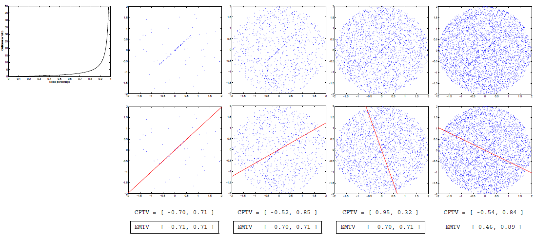
Figure 7: The top-left subfigure shows the plot of $\frac{R}{R+1}$. The four 2D data sets shown here have OI ratios $[1,20,45,80]$ respectively, which correspond to outlier percentages $[50\%,95\%,98\%,99\%]$. Our EMTV can tolerate OI ratios $\leq$ 51 in this example. The original input, the estimated line after the first EMTV iteration using CFTV to initialize the algorithm, and the line parameters after the first EMTV iteration and final EMTV convergence were shown. The ground-truth parameter is $[-0.71,0.71]$.

6.5 Implementation and Initialization

In summary, Eqns (12), (28) and (6.4) are all the equations needed to implement EMTV and therefore the implementation is straightforward.

Noting that initialization is important to an EM algorithm, to initialize EMTV, we set $\sigma_{1}$ to be a very large value, ${\mathbf{K}}_{i}=\mathbf{I}$ and $w_{i}=1$ for all $i$. ${\mathbf{S}}_{ij}^{\prime}$ is initialized to be the inverse of ${\mathbf{S}}_{ij}$, computed using the closed-form solution presented in the previous section. These initialization values mean that at the beginning we have no preference for the surface orientation. So all the input points are initially considered as inliers. With such initialization, we execute the first and the second rules in Eqn. (6.4) in sequence. Note that when the first rule is being executed, the term involving ${\mathbf{h}}$ is ignored because of the large $\sigma_{1}$, thus we can obtain ${\mathbf{K}}_{i}^{-1}$ for the second rule. After that, we can start executing the algorithm from the E-step. This initialization procedure is used in all the experiments in the following sections. Fig. 7 shows the result after the first EMTV iteration on an example; note in particular that even though the initialization is at times not close to the solution our EMTV algorithm can still converge to the desired ground-truth solution.

7 Experimental Results

First, quantitative comparison will be studied to evaluate EMTV with well-known algorithms: RANSAC [7], ASSC [28], and TV [19]. In addition, we also provide the result using the least squares method as a baseline comparison. Second, we apply our method to real data with synthetic outliers and/or noise where the ground truth is available, and perform comparison. Third, more experiments on multiview stereo matching on real images are performed.

As we will show, EMTV performed the best in highly corrupted data, because it is designed to seek one linear structure of known type (as opposed to multiple, potentially nonlinear structures of unknown type). The use of orientation constraints, in addition to position constraints, makes EMTV superior to the random sampling methods as well.

Outlier/inlier (OI) ratio  We will use the outlier/inlier (OI) ratio to characterize the outlier level, which is related to the outlier percentage $Z\in[0,1]$

$$Z=\frac{R}{R+1}$$ (33)

where $R$ is the OI ratio. Fig. 7 shows a plot of $Z=\frac{R}{R+1}$ indicating that it is much more difficult for a given method to handle the same percentage increase in outliers as the value of $Z$ increases. Note the rapid increase in the number of outliers as $Z$ increases from 50% to 99%. That is, it is more difficult for a given method to tolerate an addition of, say 20% outliers, when $Z$ is increased from 70% to 90% than from 50% to 70%. Thus the OI ratio gives more insight in studying an algorithm’s performance on severely corrupted data.

7.1 Robustness

We generate a set of 2D synthetic data to evaluate the performance on line fitting, by randomly sampling $44$ points from a line within the range $[-1,-1]\times[1,1]$ where the locations of the points are contaminated by Gaussian noise of $0.1$ standard deviation. Random outliers were added to the data with different OI ratios.

The data set is then partitioned into two:

• Set 1: OI ratio $\in[0.1,1]$ with step size 0.1,

• Set 2: OI ratio $\in[1,100]$ with step size 1.

In other words, the partition is done at 50% outliers. Note from the plot in Fig. 7 that the number of outliers increases rapidly after 50% outliers. Sample data sets with different OI ratios are shown in the top of Fig. 7. Outliers were added within a bounding circle of radius 2. In particular, the bottom of Fig. 7 shows the result of the first EMTV iteration upon initialization using CFTV.

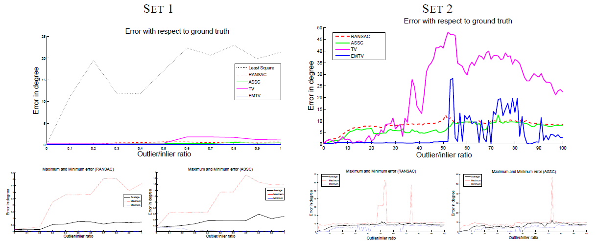
Figure 8: Error plots for Set 1 (OI ratio $=[0.1,1]$, up to 50% outliers) and Set 2 (OI ratio $=[1,100]$, $\geq$ 50% outliers). Left: for Set 1, all the tested methods except the least-squares demonstrated reliable results. EMTV is deterministic and converges quickly, capable of correcting Gaussian noise inherent in the inliers and rejecting spurious outliers, and resulting in the almost-zero error curve. Right: for Set 2, EMTV still has an almost-zero error curve up to an OI ratio of 51 ($\simeq$ 98.1% outliers). We ran 100 trials in RANSAC and ASSC and averaged the results. The maximum and minimum errors of RANSAC and ASSC are shown below each error plot.

The input scale, which is used in RANSAC, TV and EMTV, was estimated automatically by TSSE proposed in [28]. Note in principle these scales are not the same, because TSSE estimates the scales of residuals in the normal space. Therefore, the scale estimated by TSSE used in TV and EMTV are only approximations. As we will demonstrate below, even with such rough approximations, EMTV still performs very well showing that it is not sensitive to scale inaccuracy, a nice property of tensor voting which will be shown in an experiment to be detailed shortly. Note that ASSC [28] does not require any input scale.

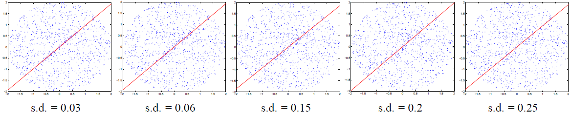
Figure 9: Inputs containing various measurement errors, with OI ratio = 10 and fixed outliers location. The estimated models (depicted by the red lines) obtained using EMTV are overlayed on the inputs. Notice the line cluster becomes less salient when s.d. = 0.25.

Set 1 – Refer to the left of Fig. 8 which shows the error produced by various methods tested on Set 1. The error is measured by the angle between the estimated line and the ground-truth. Except the least squares method, we observe that all the tested methods (RANSAC, ASSC, TV and EMTV) performed very well with OI ratios $\leq 1$. For RANSAC and ASSC, all the detected inliers were finally used in parameter estimation. Note that the errors measured for RANSAC and ASSC were the average errors in 100 executions, Fig. 8 also shows the maximum and minimum errors of the two methods after running 100 trials. EMTV does not have such maximum and minimum error plots because it is deterministic.

Observe that the errors produced by our method are almost zero in Set 1. EMTV is deterministic and converges quickly, capable of correcting Gaussian noise inherent in the inliers and rejecting spurious outliers, and resulting in the almost-zero error curve. RANSAC and ASSC have error $<0.6^{\circ}$ , which is still very acceptable.

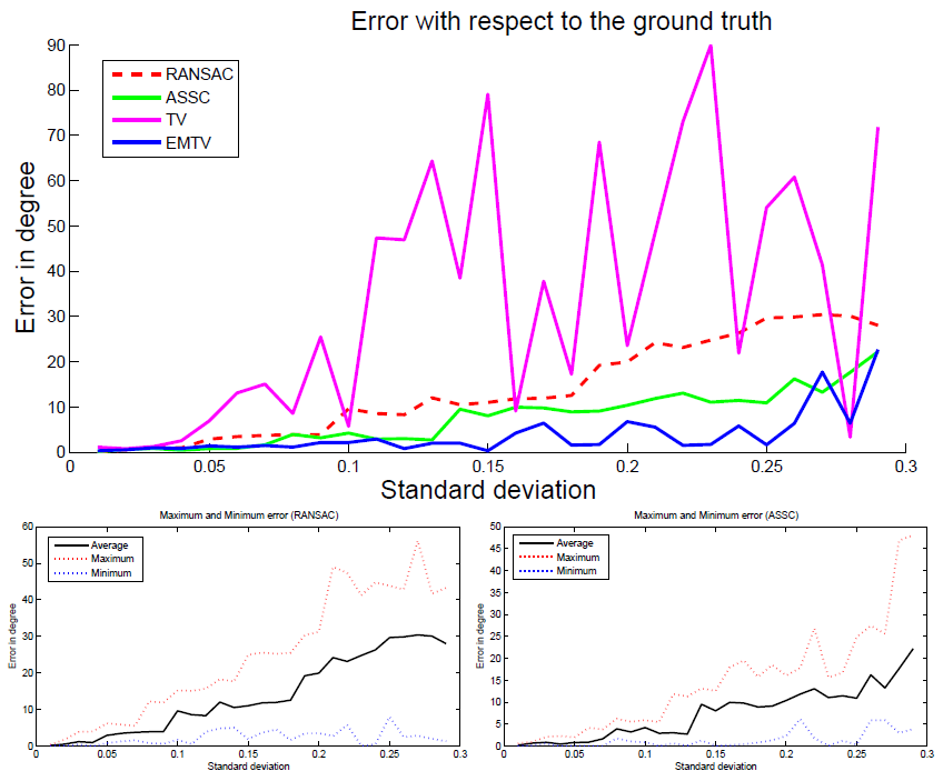
Figure 10: Measurement error: standard deviation varies from 0.01 to 0.29 with OI ratio at 10.

Set 2 – Refer to the right of Fig. 8 which shows the result for Set 2, from which we can distinguish the performance of the methods. TV breaks down at OI ratios $\geq 20$. After that, the performance of TV is unpredictable. EMTV breaks down at OI ratios $\geq$ 51, showing greater robustness than TV in this experiment due to the EM parameter fitting procedure.

The performance of RANSAC and ASSC were quite stable where the average errors are within 4 and 7 degrees over the whole spectrum of OI ratios considered. The maximum and minimum errors are shown in the bottom of Fig. 8, which shows that they can be very large at times. EMTV produces almost zero errors with OI ratio $\leq 51$, but then breaks down with unpredictable performance. From the experiments on Set 1 and Set 2 we conclude that EMTV is robust up to an OI ratio of 51 ($\simeq$98.1% outliers).

Insensitivity to choice of scale. We studied the errors produced by EMTV with different scales $\sigma_{d}$ (Eqn. (2)), given OI ratio of 10 ($\simeq$91% outliers). Even in the presence of many outliers, EMTV broke down only when $\sigma_{d}\simeq 0.7$ (the ground-truth $\sigma_{d}$ is 0.1), which indicates that our method is not sensitive to large deviations of scale. Note that the scale parameter can sometimes be automatically estimated (e.g., by modifying the original TSSE to handle tangent space) as was done in the previous experiment.

Large measurement errors. In this experiment, we increased the measurement error by increasing the standard deviation (s.d.) from 0.01 to 0.29, while keeping OI ratio equal to 10 and the location of the outliers fixed. Some of the input data sets are depicted in Fig. 9, showing that the inliers are less salient as the standard deviation (s.d.) increases. A similar experiment was also performed in [20]. Again, we compared our method with RANSAC, ASSC and TV.

According to the error plot in the top of Fig. 10, TV is very sensitive to the change of s.d.: when the s.d. is greater than 0.03, the performance is unpredictable. With increasing s.d., the performance of RANSAC and ASSC degrade gracefully while ASSC always outperforms RANSAC. The bottom of Fig. 10 shows the corresponding maximum and minimum error in 100 executions.

On the other hand, we observe the performance of EMTV (with $\sigma_{d}=0.05$) is extremely steady and accurate when s.d. $<0.15$. After that, although its error plot exhibits some perturbation, the errors produced are still small and the performance is quite stable compared with other methods.

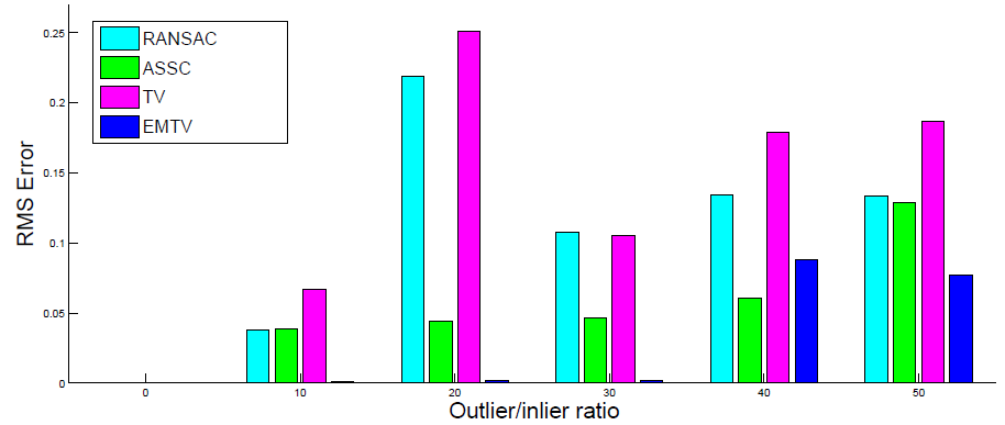
Figure 11: Corridor. RMS error plot of various methods.

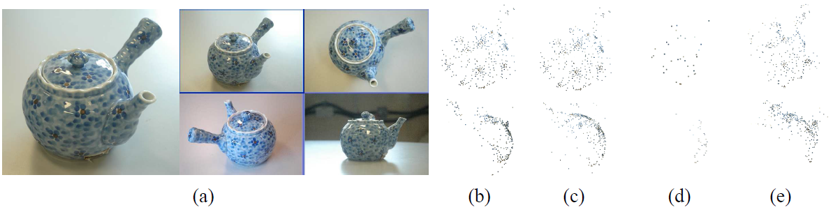
Figure 12: Teapot: (a) 4 images (one in enlarged view) from the input image set consisting of 30 images captured around the object in a casual manner. (b)–(f) show two views of the sparse reconstruction generated by using KeyMatchFull (398 points), linear_match (493 points), ransac_match (37 points), assc_match (208 points), and emtv_match (2152 points). The candidate matches returned by SIFT are extremely noisy due to the ambiguous patchy patterns. On average 17404 trials were run in ransac_match. It is time consuming to run more trials on this noisy and large input where an image pair can have as many as 5000 similar matches. Similarly for assc_match where additional running time is needed to estimate the scale parameter in each iteration. On the other hand, emtv_match does not require any random sampling.

7.2 Fundamental Matrix Estimation

Given an image pair with $p\geq 8$ correspondences ${\cal P}=\{(\mathbf{u}_{i},\mathbf{u^{\prime}}_{i})|8\leq i\leq p\}$, the goal is to estimate the $3\times 3$ fundamental matrix $\mathbf{F}=[f]_{a,b}$, where $a,b\in\{1,2,3\}$, such that

$$\mathbf{u^{\prime}}_{i}^{T}\mathbf{F}\mathbf{u}_{i}=0$$ (34)

for all $i$. $\mathbf{F}$ is of rank 2. Let $\mathbf{u}=(u,v,1)^{T}$ and $\mathbf{u^{\prime}}=(u^{\prime},v^{\prime},1)$, Eqn. (34) can be rewritten into:

$$\mathbf{U}_{i}^{T}\mathbf{h}=0$$ (35)

where

$$\mathbf{U} = (uu^{\prime},uv^{\prime},u,vu^{\prime},vv^{\prime}v,u^{\prime},v^{\prime},1)^{T}$$

$$\mathbf{v} = (f_{11},f_{21},f_{31},f_{12},f_{22},f_{32},f_{13},f_{23},f_{33})^{T}$$

Noting that Eqn. (35) is a simple plane equation, if we can detect and handle noise and outliers in the feature space, Eqn. (35) should enable us to produce a good estimation. Finally, we apply [12] to obtain a rank-2 fundamental matrix. Data normalization is similarly done as in [12] before the optimization.

We evaluate the results by estimating the fundamental matrix of the data set Corridor, which is available at www.robots.ox.ac.uk/$\sim$vgg/data.html. The matches of feature points (Harris corners) are available. Random outliers were added in the feature space.

Fig. 11 shows the plot of RMS error, which is computed by summing up and averaging $\sqrt{\frac{1}{p}\sum_{i}||\mathbf{U}_{i}^{T}\hat{\mathbf{h}}||^{2}}$ over all pairs, where $\mathbf{U}_{i}$ is the set of clean data, and $\hat{\mathbf{h}}$ is the 9D vector produced from the rank-2 fundamental matrices estimated by various methods. Note that all the images available in the Corridor data set are used, that is, all $C^{11}_{2}$ pairs were tested. It can be observed that RANSAC breaks down at an OI ratio $\simeq 20$, or 95.23% outliers. ASSC is very stable with RMS error $<0.15$. TV breaks down at an OI ratio $\simeq 10$. EMTV has negligible RMS error before it starts to break down at an OI ratio $\simeq 40$. This finding echoes that of [12] that linear solution is sufficient when outliers are properly handled.

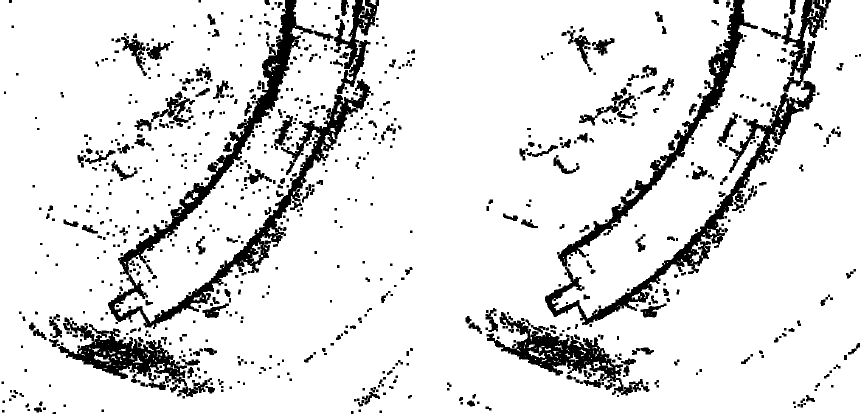
Figure 13: Results before and after filtering of Hall 3 (images shown in Fig. 14). All salient 3D structures are retained in the filtered result, including the bushes near the left facade and planters near the right facade in this top view of the building.

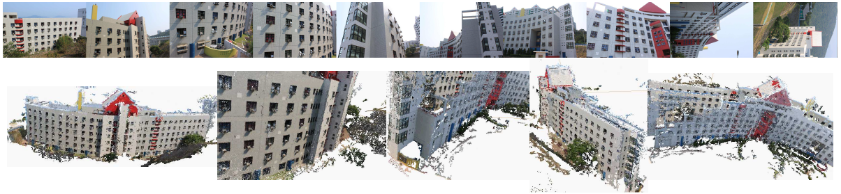
Figure 14: The Hall 3 reconstruction: ten of the input images (top) and five views of the quasi-dense 3D reconstruction (bottom).

7.3 Matching

In the uncalibrated scenario, EMTV estimates parameter accurately by employing CFTV, and effectively discards epipolar geometries induced by wrong matches. Typically, camera calibration is performed using nonlinear least-squares minimization and bundle adjustment [16] which requires good matches as input. In this experiment, candidate matches are generated by comparing the resulting 128D SIFT feature vectors [17], so many matched keypoints are not corresponding.

The epipolar constraint is enforced in the matching process using EMTV, which returns the fundamental matrix and the probability $w_{i}$ (Eqn (28)) of a keypoint pair $i$ being an inlier. In the experiment, we assume keypoint pair $i$ is an inlier if $w_{i}>0.8$. Fig. 12 shows our running example teapot which contains repetitive patterns across the whole object. Wrong matches can be easily produced by similar patterns on different parts of the teapot. This data set contains 30 images captured using a Nikon D70 camera. Automatic configuration was set during the image capture. Visually, the result produced using emtv_match is much denser than the results produced with KeyMatchFull [25], linear_match, assc_match [28], and ransac_match. Note in particular that only emtv_match recovers the overall geometry of the teapot, whereas the other methods can only recover one side of the teapot.

This example is challenging, because the teapot’s shape is quite symmetric and the patchy patterns look identical everywhere. As was done in [25], each photo was paired respectively with a number of photos with camera poses satisfying certain basic criteria conducive to matching or making the numerical process stable (e.g. wide-baseline stereo). We can regard this pair-up process as one of computing connected components. If the fundamental matrix between any successive images are incorrectly estimated, the corresponding components will no longer be connected, resulting in the situation that only one side or part of the object can be recovered.

Since KeyMatchFull and linear_match use simple distance measure for finding matches, the coverage of the corresponding connected components tend to be small. It is interesting to note that the worst result is produced by using ransac_match. This can be attributed to three reasons: (1) the fundamental matrix is of rank 2 which implies that ${\mathbf{h}}$ spans a subspace $\leq$ 8-D rather than a 9-D hyperplane; (2) the input matches contain too many outliers for some image pairs; (3) it is not feasible to fine tune the scale parameter for every possible image pair and so we used a single value for all of the images. A slight improvement could be found from ASSC. However, it still suffers from problems (1) and (2) and so the result is not very good even compared with KeyMatchFull and linear_match.

On the other hand, emtv_match utilizes the epipolar geometry constraint by computing the fundamental matrix in a data driven manner. Since the outliers are effectively filtered out, the estimated fundamental matrices are sufficiently accurate to pair up all of the images into a single connected component. Thus, the overall 3D geometry can be recovered from all the available views.

7.4 Multiview Stereo Reconstruction

This section outlines how CFTV and EMTV are applied to improve the match-propagate-filter pipeline in multiview stereo. Match-propagate-filter is a competitive approach to multiview stereo reconstruction for computing a (quasi) dense representation. Starting from a sparse set of initial matches with high confidence, matches are propagated using photoconsistency to produce a (quasi) dense reconstruction of the target shape. Visibility consistency can be applied to remove outliers. Among the existing works using the match-propagate-filter approach, patch-based multiview stereo (or PMVS) proposed in [10] has produced some best results to date.

We observe that PMVS had not fully utilized the 3D information inherent in the sparse and dense geometry before, during and after propagation, as patches do not adequately communicate among each other. As noted in [10], data communication should not be done by smoothing, but the lack of communication will cause perturbed surface normals and patch outliers during the propagation stage. In [29], we proposed tensor-based multiview stereo (TMVS) and used 3D structure-aware tensors which communicate among each other via CFTV. We found that such tensor communication not only improves propagation in MVS without undesirable smoothing but also benefits the entire match-propagate-filter pipeline within a unified framework.

We captured 179 photos around a building which were first calibrated as described in section 7.3. All images were taken on the ground level not higher than the building, so we have very few samples of the rooftop. The building facades are curved and the windows on the building look identical to each other. The patterns on the front and back facade look nearly identical. These ambiguities cause significant challenges in the matching stage especially for wide-baseline stereo. TMVS was run to obtain the quasi-dense reconstruction, where MRFTV was used to filter outliers as shown in Fig. 13. Fig. 14 shows the 3D reconstruction which is faithful to the real building. Readers are referred to [29] for more detail and experimental evaluation of TMVS.

8 Conclusions

A closed-form solution is proved for the special theory of tensor voting (CFTV) for computing an exact structure-aware tensor in any dimensions. For structure propagation, we derive a quadratic energy for MRFTV, thus providing a convergence proof for tensor voting which is impossible to prove using the original tensor voting procedure. Then, we derive EMTV for optimizing both the tensor and model parameters for robust parameter estimation. We performed quantitative and qualitative evaluation using challenging synthetic and real data sets. In the future we will develop a closed-form solution for the general theory of tensor voting, and extend EMTV to extract multiple and nonlinear structures. We have provided C$++$ source code, but it is straightforward to implement Eqns (11), (12), (28), (6.4), (18), and (19). We demonstrated promising results in multiview stereo, and will apply our closed-form solution to address important computer vision problems.

Tai-Pang Wu received the PhD degree in computer science from the Hong Kong University of Science and Technology (HKUST) in 2007. He was awarded the Microsoft Fellowship in 2006. After graduation, he has been employed as a postdoctoral fellow in Microsoft Research Asia Beijing (2007–2008) and the Chinese University of Hong Kong (2008–2010). He is currently a Senior Research at the Enterprise and Consumer Electronics Group of the Hong Kong Applied Science and Technology Research Institute (ASTRI). His research interests include computer vision and computer graphics. He is a member of the IEEE and the IEEE Computer Society.

Sai-Kit Yeung received his PhD degree in electronic and computer engineering from the Hong Kong University of Science and Technology (HKUST) in 2009. He received his BEng degree (First Class Honors) in computer engineering and MPhil degree in bioengineering from HKUST in 2003 and 2005 respectively. He is currently an Assistant Professor at the Singapore University of Technology and Design (SUTD). Prior to joining SUTD, he was a Postdoctoral Scholar in the Department of Mathematics, University of California, Los Angeles (UCLA) in 2010. His research interests include computer vision, computer graphics, computational photography, image/video processing, and medical imaging. He is a member of IEEE and IEEE Computer Society.

Jiaya Jia Jiaya Jia received the PhD degree in computer science from Hong Kong University of Science and Technology in 2004 and is currently an associate professor in Department of Computer Science and Engineering at the Chinese University of Hong Kong (CUHK). He was a visiting scholar at Microsoft Research Asia from March 2004 to August 2005 and conducted collaborative research at Adobe Systems in 2007. He leads the research group in CUHK, focusing on computational photography, 3D reconstruction, practical optimization, and motion estimation. He serves as an associate editor for TPAMI and as an area chair for ICCV 2011. He was on the program committees of several major conferences, including ICCV, ECCV, and CVPR, and co-chaired the Workshop on Interactive Computer Vision in conjunction with ICCV 2007. He received the Young Researcher Award 2008 and Research Excellence Award 2009 from CUHK. He is a senior member of the IEEE.

Chi-Keung Tang received the MSc and PhD degrees in computer science from the University of Southern California (USC), Los Angeles, in 1999 and 2000, respectively. Since 2000, he has been with the Department of Computer Science at the Hong Kong University of Science and Technology (HKUST) where he is currently a professor. He is an adjunct researcher at the Visual Computing Group of Microsoft Research Asia. His research areas are computer vision, computer graphics, and human-computer interaction. He is an associate editor of IEEE Transactions on Pattern Analysis and Machine Intelligence (TPAMI), and on the editorial board of International Journal of Computer Vision (IJCV). He served as an area chair for ACCV 2006 (Hyderabad), ICCV 2007 (Rio de Janeiro), ICCV 2009 (Kyoto), ICCV 2011 (Barcelona), and as a technical papers committee member for the inaugural SIGGRAPH Asia 2008 (Singapore), SIGGRAPH 2011 (Vancouver), and SIGGRAPH Asia 2011 (Hong Kong), SIGGRAPH 2012 (Los Angeles). He is a senior member of the IEEE and the IEEE Computer Society.

Gérard Medioni received the Diplôme d’Ingénieur from the École Nationale Supérieure des Télécommunications (ENST), Paris, in 1977 and the MS and PhD degrees from the University of Southern California (USC) in 1980 and 1983, respectively. He has been with USC since then and is currently a professor of computer science and electrical engineering, a codirector of the Institute for Robotics and Intelligent Systems (IRIS), and a codirector of the USC Games Institute. He served as the chairman of the Computer Science Department from 2001 to 2007. He has made significant contributions to the field of computer vision. His research covers a broad spectrum of the field, such as edge detection, stereo and motion analysis, shape inference and description, and system integration. He has published 3 books, more than 50 journal papers, and 150 conference articles. He is the holder of eight international patents. He is an associate editor of the Image and Vision Computing Journal, Pattern Recognition and Image Analysis Journal, and International Journal of Image and Video Processing. He served as a program cochair of the 1991 IEEE Computer Vision and Pattern Recognition (CVPR) Conference and the 1995 IEEE International Symposium on Computer Vision, a general cochair of the 1997 IEEE CVPR Conference, a conference cochair of the 1998 International Conference on Pattern Recognition, a general cochair of the 2001 IEEE CVPR Conference, a general cochair of the 2007 IEEE CVPR Conference, and a general cochair of the upcoming 2009 IEEE CVPR Conference. He is a fellow of the IEEE, IAPR, and AAAI and a member of the IEEE Computer Society.

Tai-Pang Wu, Sai-Kit Yeung, Chi-Keung Tang^∗Please direct all inquiries to the contact author. E-mail: cktang@cse.ust.hk,

Jiaya Jia and Gerard Medioni

Addendum

A closed-form solution to tensor voting or CFTV was proved in [2]. With CFTV, discrete voting field is no longer required where uniform sampling, computation and storage efficiency are issues in high dimensional inference.

We respond to the comments paper [1] on the proof to the closed-form solution to tensor voting [2] or CFTV. First, the proof is correct and let ${\mathbf{S}}$ be the resulting tensor which may be asymmetric. Second, ${\mathbf{S}}$ should be interpreted using singular value decomposition (SVD), where the symmetricity of ${\mathbf{S}}$ is unimportant, because the corresponding eigensystems to the positive semidefinite (PSD) systems, namely, ${\mathbf{S}}{\mathbf{S}}^{T}$ or ${\mathbf{S}}^{T}{\mathbf{S}}$, are used in practice. Finally, we prove a symmetric version of CFTV, run extensive simulations and show that the original tensor voting, the asymmetric CFTV and symmetric CFTV produce practically the same empirical results in tensor direction except in high uncertainty situations due to ball tensors and low saliency.

Dirty codes for the experimental section to show the practical equivalence of the asymmetric CFTV, symmetric CFTV, and original discrete tensor voting (that is, Eq. (2)) in 2D are available.

1 Asymmetric CFTV

We reprise here the main result in [2] in an equivalent form:

Theorem 1

(Closed-Form Solution to Tensor Voting) The tensor vote at ${\mathbf{x}}_{i}$ induced by ${\mathbf{K}}_{j}$ located at ${\mathbf{x}}_{j}$ is given by the following closed-form solution:

$${\mathbf{S}}_{ij}=c_{ij}{\mathbf{R}}_{ij}\left({\mathbf{K}}_{j}-\frac{1}{2}{\mathbf{K}}_{j}\mathbf{r}_{ij}\mathbf{r}_{ij}^{T}\right){\mathbf{R}}^{T}_{ij}$$ (36)

where ${\mathbf{K}}_{j}$ is a second-order symmetric tensor, ${\mathbf{R}}_{ij}={\mathbf{I}}-2{\mathbf{r}}_{ij}{\mathbf{r}}_{ij}^{T}$, ${\mathbf{I}}$ is an identity, ${\mathbf{r}}_{ij}$ is a unit vector pointing from ${\mathbf{x}}_{j}$ to ${\mathbf{x}}_{i}$ and $c_{ij}=\exp(-\frac{||{\mathbf{x}}_{i}-{\mathbf{x}}_{j}||^{2}}{\sigma_{d}})$ with $\sigma_{d}$ as the scale parameter.

To simplify notation we will drop the subscripts in ${\mathbf{R}}$ and $\mathbf{r}$, and let ${\mathbf{T}}=\frac{1}{2}{\mathbf{K}}_{j}\mathbf{r}\mathbf{r}^{T}$.

In [1] an example is given: for an input PSD ${\mathbf{K}}_{j}=\left[\begin{array}[]{cc}\frac{1}{2}&0\\ 0&1\end{array}\right]$, the output ${\mathbf{S}}$ computed using Theorem 1 is asymmetric, much less that ${\mathbf{S}}$ is a PSD matrix. It was also pointed out in [1] potential technical flaws involving the derivative with respect to a unit stick tensor in the proof to Theorem 1, which is related to Footnote 3 in [2].

Note that Theorem 1 does not guarantee the output ${\mathbf{S}}$ is symmetric or PSD. In the C codes accompanying [2], which is available in the IEEE digital library, the eig_sys function behaves like singular value decomposition svd. The statements and experiments pertinent to ${\mathbf{S}}$ in [2] subsequent to Theorem 1 in fact refer to the SVD results on ${\mathbf{S}}$, and we apologize for not making this explicitly clear in the paper.

Recall the singular value decomposition and the eigen-decomposition are related, namely, the left-singular vectors of ${\mathbf{S}}$ are eigenvectors of ${\mathbf{S}}{\mathbf{S}}^{T}$, the right singular-vectors of ${\mathbf{S}}$ are eigenvectors of ${\mathbf{S}}^{T}{\mathbf{S}}$, where the eigenvectors are orthonormal bases. We performed sanity check by running extensive simulations in dimensions up to 51 and show that all eigenvalues of ${\mathbf{S}}{\mathbf{S}}^{T}$ and ${\mathbf{S}}^{T}{\mathbf{S}}$ are nonnegative, and that they are PSD. The symmetricity of ${\mathbf{S}}$ is unimportant in practice.

Nonetheless, for theoretical interest we provide in the following an alternative proof to Theorem 1 which produces a symmetric ${\mathbf{S}}$ and serves to dispel the flaws pointed out in [1]. Finally we run simulations to show that the original tensor voting, the asymmetric CFTV in [2] and the symmetric CFTV in the following produce the practically the same results.

2 Symmetric CFTV

From the first principle, integrating unit stick tensors $\mathbf{N}_{\theta}=\mathbf{n}_{\theta}\mathbf{n}_{\theta}^{T}$ in all directions $\theta$ with strength $\tau_{\theta}^{2}$, we obtain Eq. (8) in [2]:

$${\mathbf{S}}_{ij} = c_{ij}\mathbf{R}\left(\mathbf{K}_{j}-\int_{\mathbf{N}_{\theta}\in\nu}\tau_{\theta}^{2}\mathbf{N}_{\theta}\mathbf{r}\mathbf{r}^{T}\mathbf{N}_{\theta}d\mathbf{N}_{\theta}\right)\mathbf{R}^{T}$$ (37)

Note the similar form of Eqs (36) and (37), and the unconventional integration domain in Eq. (37) where $\nu$ represents the space of stick tensors given by $\mathbf{n}_{\theta j}$ as explained in [2]. Let $\Omega$ be the integration domain to shorten our notations.

Let ${{\mathbf{T}}}_{\mathit{sym}}$ be the integration in Eq. (37). ${\mathbf{T}}_{\mathit{sym}}$ can be solved by integration by parts. Here, we repeat Footnote 3 in [2] on the contraction of a sequence of identical unit stick tensors when multiplied together. Let $\mathbf{N}_{\theta}=\mathbf{n}_{\theta}\mathbf{n}_{\theta}^{T}$ be a unit stick tensor, where $\mathbf{n}_{\theta}$ is a unit normal at angle $\theta$, and $q\geq 1$ be a positive integer, then

$$\mathbf{N}_{\theta}^{q}=\mathbf{n}_{\theta}\mathbf{n}_{\theta}^{T}\mathbf{n}_{\theta}\mathbf{n}_{\theta}^{T}\cdots\mathbf{n}_{\theta}\mathbf{n}_{\theta}^{T}=\mathbf{n}_{\theta}\cdot 1\cdot 1\cdots 1\cdot\mathbf{n}_{\theta}^{T}=\mathbf{n}_{\theta}\mathbf{n}_{\theta}^{T}=\mathbf{N}_{\theta}.$$ (38)

To preserve symmetry, we leverage Footnote 3 or Eq. (38) above but rather than exclusively using contraction, (i.e., $\mathbf{N}_{\theta}^{q}=\mathbf{N}_{\theta}$) as done in [2], we use expansion (i.e., $\mathbf{N}_{\theta}=\mathbf{N}_{\theta}^{q}$) in the following:

$${\mathbf{T}}_{\mathit{sym}}=\int_{\Omega}\tau_{\theta}^{2}\mathbf{N}_{\theta}\mathbf{r}\mathbf{r}^{T}\mathbf{N}_{\theta}d\mathbf{N}_{\theta}=\int_{\Omega}\tau_{\theta}^{2}\mathbf{N}_{\theta}^{2}\mathbf{r}\mathbf{r}^{T}\mathbf{N}_{\theta}^{2}d\mathbf{N}_{\theta}$$ (39)

Let $f(\theta)=\tau_{\theta}^{2}\mathbf{N}_{\theta}^{2}$, then $f^{\prime}(\theta)=2\tau_{\theta}^{2}\mathbf{N}_{\theta}d\mathbf{N}_{\theta}=2\tau_{\theta}^{2}\mathbf{N}_{\theta}^{2}d\mathbf{N}_{\theta}$ after expansion. Similarly, let $g(\theta)=\frac{1}{2}\mathbf{r}\mathbf{r}^{T}\mathbf{N}_{\theta}^{2}$ and $g^{\prime}(\theta)=\mathbf{r}\mathbf{r}^{T}\mathbf{N}_{\theta}d\mathbf{N}_{\theta}=\mathbf{r}\mathbf{r}^{T}\mathbf{N}_{\theta}^{2}d\mathbf{N}_{\theta}$ after expansion. Note also ${\mathbf{K}}_{j}$, in the most general form, can be expressed as $\int_{\Omega}\tau_{\theta}^{2}\mathbf{N}_{\theta}d\mathbf{N}_{\theta}$. So, we obtain

$${{\mathbf{T}}}_{\mathit{sym}} = \int_{\Omega}\tau_{\theta}^{2}\mathbf{N}_{\theta}^{2}\mathbf{r}\mathbf{r}^{T}\mathbf{N}_{\theta}^{2}d\mathbf{N}_{\theta}$$

$$= \left[f(\theta)g(\theta)\right]_{\Omega}-\int_{\Omega}f^{\prime}(\theta)g(\theta)d\mathbf{N}_{\theta}$$

$$= \left[\frac{1}{2}\tau_{\theta}^{2}\mathbf{N}_{\theta}^{2}\mathbf{r}\mathbf{r}^{T}\mathbf{N}_{\theta}^{2}\right]_{\Omega}-\int_{\Omega}\tau_{\theta}^{2}\mathbf{N}_{\theta}^{2}\mathbf{r}\mathbf{r}^{T}\mathbf{N}_{\theta}^{2}d\mathbf{N}_{\theta}$$

$$= \left[\frac{1}{2}\tau_{\theta}^{2}\mathbf{N}_{\theta}^{2}\mathbf{r}\mathbf{r}^{T}\mathbf{N}_{\theta}^{2}\right]_{\Omega}-{\mathbf{T}}_{\mathit{sym}}$$

$$= \frac{1}{4}\left[\tau_{\theta}^{2}\mathbf{N}_{\theta}^{2}\mathbf{r}\mathbf{r}^{T}\mathbf{N}_{\theta}^{2}\right]_{\Omega}$$

$$= \frac{1}{4}\int_{\Omega}\left(\tau_{\theta}^{2}\frac{d}{d{\mathbf{N}}_{\theta}}[{\mathbf{N}}_{\theta}^{2}]{\mathbf{r}}{\mathbf{r}}^{T}{\mathbf{N}}_{\theta}^{2}+\tau_{\theta}^{2}{\mathbf{N}}_{\theta}^{2}\frac{d}{d{\mathbf{N}}_{\theta}}[{\mathbf{r}}{\mathbf{r}}^{T}{\mathbf{N}}_{\theta}^{2}]\right)d{\mathbf{N}}_{\theta}$$

$$= \frac{1}{4}\int_{\Omega}\left(\tau_{\theta}^{2}\frac{d}{d{\mathbf{N}}_{\theta}}[{\mathbf{N}}_{\theta}]{\mathbf{r}}{\mathbf{r}}^{T}{\mathbf{N}}_{\theta}+\tau_{\theta}^{2}{\mathbf{N}}_{\theta}\frac{d}{d{\mathbf{N}}_{\theta}}[{\mathbf{r}}{\mathbf{r}}^{T}{\mathbf{N}}_{\theta}]\right)d{\mathbf{N}}_{\theta}$$

$$= \frac{1}{4}\int_{\Omega}\left(\mathbf{r}\mathbf{r}^{T}\tau_{\theta}^{2}\mathbf{N}_{\theta}+\tau_{\theta}^{2}\mathbf{N}_{\theta}\mathbf{r}\mathbf{r}^{T}\right)d{\mathbf{N}}_{\theta}$$ (41)

$$= \frac{1}{4}\left(\mathbf{r}\mathbf{r}^{T}{\mathbf{K}}_{j}+{\mathbf{K}}_{j}\mathbf{r}\mathbf{r}^{T}\right).$$

Here, in the derivative with respect to a unit stick tensor $\mathbf{N}_{\theta}$ along the tensor direction, the tensor magnitude $\tau_{\theta}^{2}$ can be legitimately regarded as a constant.

Note that we apply contraction in Eq. (41). Comparing the pertinent ${\mathbf{T}}$ in the asymmetric CFTV in Eq. (36) and symmetric CFTV in Eq. (41):

$${\mathbf{T}}_{\mathit{asym}} = \frac{1}{2}{\mathbf{K}}_{j}\mathbf{r}\mathbf{r}^{T}$$

$${\mathbf{T}}_{\mathit{sym}} = \frac{1}{4}\left(\mathbf{r}\mathbf{r}^{T}{\mathbf{K}}_{j}+{\mathbf{K}}_{j}\mathbf{r}\mathbf{r}^{T}\right)$$

it is interesting to observe how tensor contraction and expansion when applied as described can preserve tensor symmetry whereas in [2], only tensor contraction was applied.

Notwithstanding, the symmetricity of ${\mathbf{S}}$ is unimportant in practice as singular value decomposition will be applied to ${\mathbf{S}}$ before the eigenvalues and eigenvectors are used. The following section reports the results of our experiments on the asymmetric and symmetric CFTV when used in practice.

3 Experiments

In each of the following simulations, a random input PSD matrix ${\mathbf{K}}={\mathbf{A}}{\mathbf{A}}^{T}+\epsilon{\mathbf{I}}$ is generated, where ${\mathbf{A}}$ is a random square matrix, ${\mathbf{I}}$ is an identity, $\epsilon$ is a small constant (e.g. $1e^{-2})$.

1. (Sanity check) $N$D simulations ($N=2$ to $51$) of $1000$ tensors for each dimension

   1. The ${\mathbf{S}}$ produced by symmetric CFTV is indeed symmetric. This is confirmed by testing each ${\mathbf{S}}$ using ${\mathit{n}orm}({\mathbf{S}}^{-1}{\mathbf{S}}^{T}-{\mathbf{I}})=0$, where ${\mathit{n}orm}(\cdot)$ is the $L_{2}$ norm of a matrix.

   2. ${\mathbf{S}}^{T}{\mathbf{S}}$ and ${\mathbf{S}}{\mathbf{S}}^{T}$ are PSD where ${\mathbf{S}}$ can be produced by asymmetric or symmetric CFTV. This is validated by checking all eigenvalues being nonnegative.

2. 2D simulations of more than 1 million tensors show the practical equivalence in tensor direction among

   1. discrete solution to original tensor voting Eq. (37), or Eq. (8) in [2],

   2. ${\mathbf{S}}^{T}{\mathbf{S}}$ and ${\mathbf{S}}{\mathbf{S}}^{T}$ produced by asymmetric CFTV,

   3. ${\mathbf{S}}^{T}{\mathbf{S}}$ ($={\mathbf{S}}{\mathbf{S}}^{T}$ when ${\mathbf{S}}$ is symmetric) produced by symmetric CFTV,

   while relative tensor saliency is preserved.

3. $N$D simulations ($N=2$ to $51$) of $1000$ tensors for each dimension show the practical equivalence in tensor direction among

   1. ${\mathbf{S}}^{T}{\mathbf{S}}$ and ${\mathbf{S}}{\mathbf{S}}^{T}$ produced by asymmetric CFTV,

   2. ${\mathbf{S}}^{T}{\mathbf{S}}$ ($={\mathbf{S}}{\mathbf{S}}^{T}$) produced by symmetric CFTV,

   in their largest eigenvectors which encompass the most “energy” while the rest represents uncertainty in orientation each spanning a plane perpendicular to the largest eigenvectors.

For simulations in (2), we exclude ball tensors from our tabulation for the obvious reason: any two orthonormal vectors describe the equivalent unit ball tensor. The mean and maximum deviation in tensor direction are respectively 0.9709 and 0.9537 (score for perfect alignment is 1) in terms of the dot product among the relevant eigenvectors. The deviation can be explained by the imperfect uniform sampling for a 2D ellipse used in computing the discrete tensor voting solution: there is no good way for uniform sampling in $N$ dimensions. When we turned off the discrete tensor voting but compared only the asymmetric and symmetric CFTV, the mean and maximum deviation in tensor direction are respectively improved to 0.9857 and 0.9718.

For tensor saliency, we found that while the normalized saliencies are not identical among the four versions of tensor voting , their relative order is preserved. That is, when we sort the eigenvectors according to their corresponding eigenvalues in the respective implementation of tensor voting, the sorted eigenvectors are always empirically identical among the four cases.

For simulations in (3), we did not compare the discrete solution: in higher dimensions, uniform sampling of an $N$D ellipsoid is an issue to discrete tensor voting. The mean and maximum deviation among the largest eigenvector of the three versions are respectively 0.9940 and 0.9857.

4 Epilogue

We revisit the main result in [2], and reconfirm the efficacy of the closed-form solution to tensor voting which votes for the most likely connection without discrete voting fields, which is particularly relevant in high dimensional inference where uniform sampling and storage of discrete voting fields are issues. As an aside, we prove the symmetric version of CFTV.

The application of tensor contraction and expansion given by Eq. (38) is instrumental to the derivation of the closed-form solution. Interestingly, while ${\mathbf{S}}$ may be asymmetric, pre-multiplying or post-multiplying by itself not only echos the contraction/expansion operation given by Eq. (38) but also produces a PSD system that agrees with the original tensor voting result. As shown above, the inherent flexibility also makes symmetric CFTV possible. Thus we believe further exploration may lead to useful and interesting theoretical results on tensor voting.

References

- [1] S. Arya and D. M. Mount. Approximate nearest neighbor searching. ACM-SIAM SODA’93, pages 271–280.
- [2] J. Bilmes. A gentle tutorial on the EM algorithm and its application to parameter estimation for Gaussian mixture and hidden Markov models. Technical Report ICSI-TR-97-021, ICSI, 1997.
- [3] H. Chen and P. Meer. Robust regression with projection based m-estimators. In ICCV03, pages II: 878–885, 2003.
- [4] O. Chum and J. Matas. Optimal randomized ransac. PAMI, 30(8):1472–1482, August 2008.
- [5] D. Comaniciu and P. Meer. Mean shift: A robust approach toward feature space analysis. PAMI, 24:603–619, May 2002.
- [6] R. Dahyot. Statistical hough transform. PAMI, 31(8):1502–1509, August 2009.
- [7] M. A. Fischler and R. C. Bolles. Random sample consensus: A paradigm for model fitting with applications to image analysis and automated cartography. Comm. of the ACM, 24:381–395, 1981.
- [8] D. Forsyth and J. Ponce. Computer Vision: A Modern Approach. Prentice Hall, 2003.
- [9] E. Franken, M. van Almsick, P. Rongen, L. Florack, and B. ter Haar Romeny. An efficient method for tensor voting using steerable filters. In ECCV06, pages IV: 228–240, 2006.
- [10] Y. Furukawa and J. Ponce. Accurate, dense, and robust multiview stereopsis. PAMI, 32(8):1362–1376, August 2010.
- [11] B. Georgescu, I. Shimshoni, and P. Meer. Mean shift based clustering in high dimensions: A texture classification example. In ICCV03, pages 456–463, 2003.
- [12] R. Hartley. In defense of the eight-point algorithm. PAMI, 19(6):580–593, June 1997.
- [13] P. Hough. Machine analysis of bubble chamber pictures. Centre Européenne pour la Recherch Nucléaire (CERN), 1959.
- [14] P. J. Huber. Robust Statistics. John Wiley & Sons, 1981.
- [15] K. Lee, P. Meer, and R. Park. Robust adaptive segmentation of range images. PAMI, 20(2):200–205, February 1998.
- [16] M. Lourakis and A. Argyros. The design and implementation of a generic sparse bundle adjustment software package based on the levenberg-marquardt algorithm. In Technical Report 340, 2004.
- [17] D. Lowe. Distinctive image features from scale-invariant keypoints. IJCV, 60(2):91–110, November 2004.
- [18] G. J. McLachlan and T. Krishnan. EM Algorithms and Extension. Elsevier, 1997.
- [19] G. Medioni, M. S. Lee, and C. K. Tang. A Computational Framework for Segmentation and Grouping. Elsevier, 2000.
- [20] P. Meer. Robust techniques for computer vision. In Emerging Topics in Computer Vision, page Chapter 4, 2004.
- [21] P. Mordohai and G. Medioni. Dimensionality estimation, manifold learning and function approximation using tensor voting. JMLR, 11:411–450, January 2010.
- [22] P. Rousseeuw. Least median of squares regression. Journal of American Statistics Assoc., 79:871–880, 1984.
- [23] P. Rousseeuw. Robust Regression and Outlier Detection. Wiley, 1987.
- [24] K. Sim and R. Hartley. Removing outliers using the l-inf norm. In CVPR06, pages I: 485–494, 2006.
- [25] N. Snavely, S. Seitz, and R. Szeliski. Modeling the world from internet photo collections. IJCV, 80(2), November 2008.
- [26] R. Subarao and P. Meer. Beyond ransac: User independent robust regression. In Workshop on 25 Years of RANSAC, June 2006.
- [27] W. S. Tong, C. K. Tang, and G. Medioni. Simultaneous two-view epipolar geometry estimation and motion segmentation by 4d tensor voting. PAMI, 26(9):1167–1184, September 2004.
- [28] H. Wang and D. Suter. Robust adaptive-scale parametric model estimation for computer vision. PAMI, 26(11):1459–1474, Nov 2004.
- [29] T. P. Wu, S. K. Yeung, J. Jia, and C. K. Tang. Quasi-dense 3D reconstruction using tensor-based multiview stereo. In CVPR10, 2010.

References

- [1] E. Maggiori, P. Lotito, H. L. Manterola, and M. del Fresno. Comments on “a closed-form solution to tensor voting: Theory and applications”. IEEE Transactions on Pattern Analysis and Machine Intelligence, 36(12), 2014.
- [2] T.-P. Wu, S.-K. Yeung, J. Jia, C.-K. Tang, and G. Medioni. A closed-form solution to tensor voting: Theory and applications. IEEE Transactions on Pattern Analysis and Machine Intelligence, 34(8):1482–1495, 2012.