A model for the energy-dependent time-lag and rms of the heartbeat oscillations in GRS 1915+105

Abstract

Energy dependent phase lags reveal crucial information about the causal relation between various spectral components and about the nature of the accretion geometry around the compact objects. The time-lag and the fractional root mean square (rms) spectra of GRS 1915+105 in its heartbeat oscillation class/$\rho$ state show peculiar behaviour at the fundamental and harmonic frequencies where the lags at the fundamental show a turn around at $\sim$ 10 keV while the lags at the harmonic do not show any turn around at least till $\sim$ 20 keV. The magnitude of lags are of the order of few seconds and hence cannot be attributed to the light travel time effects or Comptonization delays. The continuum X-ray spectra can roughly be described by a disk blackbody and a hard X-ray power-law component and from phase resolved spectroscopy it has been shown that the inner disk radius varies during the oscillation. Here, we propose that there is a delayed response of the inner disk radius (DROID) to the accretion rate such that $r_{in}(t)\propto\dot{m}^{\beta}(t-\tau_{d})$. The fluctuating accretion rate drives the oscillations of the inner radius after a time delay $\tau_{d}$ while the power-law component responds immediately. We show that in such a scenario a pure sinusoidal oscillation of the accretion rate can explain not only the shape and magnitude of energy dependent rms and time-lag spectra at the fundamental but also the next harmonic with just four free parameters.

1 Introduction

GRS 1915+105 exhibits a range of variability in its light curve and power density spectra (PDS), along with other peculiar features like near-Eddington accretion rate consistent for 20 years, jet activities $-$ from steady radio flickering to super-luminal radio ejections (Mirabel & Rodriguez, 1994) and regular transitions into various spectral states in time-scale from msec to hours (Morgan, Remillard & Greiner, 1997; Muno, Morgan & Remillard, 1997; Mirabel & Rodriguez, 1994; Belloni et al, 1997). The timing analysis features 14 variability classes with each having their own peculiar light curves, phase/time-lags and coherence (Belloni et al, 1997; Pahari et al., 2013a, b). Among the 14 variability classes, the $\rho$ class shows characteristic limit-cycle variability in the time-scale of 50$-$100 sec with large amplitude oscillations in X$-$ray intensity by nearly an order of magnitude (Taam, Chen & Swank, 1997; Belloni et al, 1997).

A promising model for the $\rho$ class variability is that it is driven by radiation pressure instability (Lightman & Eardley, 1974; Taam & Lin, 1984; Taam, Chen & Swank, 1997). However, numerical simulations of the instability suggests that there is need to change the viscous prescription and take into account a fraction of energy dissipating in a corona to explain the overall X-ray modulation (e.g. Nayakshin, Rappaport, & Melia, 2000; Janiuk, Czerny, & Siemiginowska, 2000; Janiuk & Czerny, 2005). Phase resolved spectroscopy of the variability reveals a consistent picture where the instability causes the inner disk radius to vary with the luminosity variation, which may be due to mass ejection from the system (Neilsen et al., 2011, 2012). The spectral modeling at different phases show complex components consisting of disk emission and a power-law with a high energy cutoff.

Figure 1: The predicted time-lag and rms versus energy for the fundamental (left panels) and the next harmonic (right panels) for different values of the power-law to disk flux ratio parameter $N$. The other parameters are kept at some constant fiduciary values. Note the sensitivity of the peak of the time-lag curve for the fundamental to $N$.

An alternate approach to phase resolved spectroscopy is to understand the energy dependent phase lag and rms spectra of an oscillation. This is particularly useful for Quasi periodic oscillations (QPO). Such analysis of high frequency QPOs can give crucial information regarding the size of the emitting region (e.g. Lee, Misra & Taam, 2001; Kumar & Misra, 2014) and for the low frequency ones the causal connection between spectral parameters (Misra & Mondal, 2013). Ingram & van der Klis (2015) have considered both energy dependent rms and phase resolved spectroscopy to argue that the low frequency QPO in the $\chi$ state has a geometric origin. Frequency resolved spectroscopy at the QPO frequency which is related to the energy dependent rms curves can provide crucial information regarding the nature of the oscillation (Axelsson, Done, & Hjalmarsdotter, 2014). Janiuk & Czerny (2005) report hard photon time-lags for the $\rho$ class variability which they interpret as the delay for the corona to adjust to a varying accretion rate. Indeed the magnitude of the time delays of the order of seconds implies that it is not due to light travel time effects and instead should be associated with time delays between different structural parameters. Since the inner disk radius is known to vary during the oscillation (Neilsen et al., 2012), it would be interesting to see if energy dependent time-lags and the rms spectra of the different harmonics of the oscillation can provide insight into how the the inner radius varies with the accretion rate.

As we describe below the time-lag and rms spectra for the $\rho$ class variability is fairly complex and our motivation is to identify the simplest model which can describe not only the behaviour of the fundamental but also simultaneously that of the next harmonic.

2 The Delayed Response of the Inner Disk Model(DROID)

Figure 2: The predicted time-lag and rms versus energy for the fundamental (left panels) and the next harmonic (right panels) for different values of the parameter $\beta$ which relates the dependence of the inner radius with the accretion rate. The other parameters are kept at some constant fiduciary values. Note the sensitivity of the time-lag curve for the next harmonic to $\beta$.

We assume that the X$-$ray emission primarily consists of two components, a soft disk blackbody and a hard X$-$ray power-law extending from $\sim$ 1 keV to high energies due to a corona. We neglect contributions from the Iron line emission and other reflection features..

Figure 3: The predicted time-lag and rms versus energy for the fundamental (left panels) and the next harmonic (right panels) for different values of the power-law index $p$. The other parameters are kept at some constant fiduciary values.

The blackbody disk flux is given by

$$F_{d}\propto E^{2}\int_{r_{in}}^{\infty}\frac{r}{exp(\frac{E}{kT(r)})-1}dr$$ (1)

where $E$ is the energy of the photon, $r$ is the radius, $r_{in}$ is the inner disk radius and T(r) is the surface disk temperature. From the standard disk blackbody model, we have (Frank, King & Raine, 2002):

$$kT_{r}=kT_{in}\left(\frac{r}{r_{in}}\right)^{-3/4}$$ (2)

where $T_{in}\propto\dot{m}^{1/4}{r_{in}}^{-3/4}$, $\dot{m}$ is the accretion rate. The power-law component is taken to be

$$F_{p}\propto{\dot{m}}^{\Gamma}E^{-P}$$ (3)

where it has been assumed that the normalization of the power-law depends on the accretion rate ($\propto{\dot{m}}^{\Gamma}$) while for simplicity the photon index $P$ does not vary.

The variation of the total flux $F_{T}=F_{d}+F_{p}$ due to variations of the accretion rate and inner radius, to second order is given by

$$\delta F_{t} = (F_{t})_{\dot{m}}\delta{\dot{m}}+{(F_{t})_{r_{in}}}\delta{r_{in}}+\frac{1}{2}(F_{t})_{\dot{m}\dot{m}}\delta{\dot{m}^{2}}$$ (4)

$$+(F_{t})_{\dot{m}r_{in}}\delta{\dot{m}}\delta{r_{in}}+\frac{1}{2}(F_{t})_{r_{in}r_{in}}\delta{r_{in}}^{2}$$

Here we denote the normalized variation $\delta X=\Delta X/X$ and define

$$(Z)_{X}=\frac{X}{Z}\frac{\partial Z}{\partial X}\;\;\;\;\hbox{and}\;\;\;\;(Z)_{XY}=\frac{XY}{Z}\frac{\partial}{\partial X}\frac{\partial Z}{\partial Y}$$ (5)

We assume that the inner disk radius follows the accretion rate with a time delay defined by:

$$r_{in}(t)\propto\dot{m}^{-\beta}(t-\tau_{d})$$ (6)

and that the accretion rate undergoes a pure sinusoidal variation at an angular frequency $\omega$

$$\dot{m}(t)=\dot{m_{o}}(1+\delta\dot{m})=\dot{m_{o}}(1+|\delta\dot{m}|e^{i\omega t})$$ (7)

which drives the variability of the inner radius, $r_{in}(t)=r_{ino}(1+\delta r_{in})$ where

$$\delta r_{in}=-\beta|\delta\dot{m}|e^{i\omega(t-\tau_{d})}+\frac{\beta(\beta+1)}{2}|\delta\dot{m}|^{2}e^{2i\omega(t-\tau_{d})}$$ (8)

Substituting the above in Eqn (4), and collecting terms proportional to $e^{i\omega t}$ and $e^{2i\omega t}$, for the fundamental oscillation, we get:

$$\delta F_{t}^{f}=\frac{|\delta\dot{m}|}{1+\frac{F_{p}}{F_{d}}}\left(Ae^{i\omega t}+Be^{i\omega(t-\tau_{d})}\right)$$ (9)

and for the next harmonic:

$$\delta F_{t}^{h}=\frac{|\delta\dot{m}|^{2}}{1+\frac{F_{p}}{F_{d}}}\left(A^{\prime}e^{2i\omega t}+B^{\prime}e^{2i\omega(t-\tau_{d})}+C^{\prime}e^{2i\omega(t-\tau_{d}/2)}\right)$$ (10)

The coefficients $A,B,A^{\prime},B^{\prime}$ and $C^{\prime}$ are derived and listed in Appendix (A). The ratio of the power-law to disk flux $F_{p}/F_{d}$ can be conveniently written as

$$\frac{F_{p}}{F_{d}}=NG(E,kT_{in},P)$$ (11)

The function $G$ is given in Appendix B and $N$ is a parameter which can be obtained from the time-averaged spectrum.

The energy dependent rms for the fundamental and next harmonic are given by $\frac{1}{\sqrt{2}}|\delta F_{t}^{f}(E)|$ and $\frac{1}{\sqrt{2}}|\delta F_{t}^{h}(E)|$ while the phase lag with respect to a reference energy $E_{ref}$ is given by the phase of $\delta F_{t}^{f}(E)(\delta F_{t}^{f}(E_{ref}))^{*}$ and $\delta F_{t}^{h}(E)(\delta F_{t}^{h}(E_{ref}))^{*}$.

The energy dependent variations $\delta F_{t}^{f}$ and $\delta F_{t}^{h}$ given by Equations (9) and (10) depend on several parameters which can be divided into two groups. The parameters of the first group can be estimated from the time averaged spectrum which are the inner disk temperature $T_{in}$, the high energy photon index $P$ and $N$ which parametrizes the ratio of the power-law to disk flux. The parameters of the second group pertain to the nature of the oscillation and are the exponents for inner disk radius ($\beta$), the power-law flux ($\Gamma$) with the accretion rate, $\omega t_{d}$ which is the phase difference (between the inner disk radius & the accretion rate) and an over all normalization of the variation $|\delta\dot{m}|$. Thus in this simplistic model, the energy dependent rms and time-lag for the fundamental and next harmonic are completely specified by these four parameters. Of these the normalization of the variability $|\delta\dot{m}|$ determines the normalization of the rms of the fundamental while its square determines that of the next harmonic.

To illustrate the dependence of the predicted energy dependent rms and lag of this model on parameters, we show as an example in Figure (1) the predicted curves for different values of the power-law to disk flux ratio characterized by $N$ while the other parameters of the model are fixed at some fiduciary values i.e. $T_{in}$, $\beta$, $p$, $\omega*\tau_{d}$, $\Gamma$ & $\Delta\dot{m}$ at $1.5$ keV, $0.65$, $2.7$, $2.2$ ,$0.05$ and $0.4$ respectively. A salient feature of the model is that the time-lag increases with energy and then decreases. This occurs because the high energy photons are dominated by the power-law component which varies with the accretion rate without any time-delay. On the other hand, the low energy photons from the disk component are more sensitive to the accretion rate rather than the inner radius. Thus the low energy photons from the disk and the high energy ones from the power-law component have relatively less time delay as compared to photons with energy close to $T_{in}$, which depend significantly on the inner radius which is assumed to be delayed with respect to the accretion rate. Thus, the turnover energy depends sensitively on the flux ratio of the power-law and disk components characterized by the parameter $N$. Since the ratio can be estimated from the time-averaged spectrum, there is little leverage to tune the other parameters to get the observed lag turnover energy.

In Figure (2), we show the rms and time-lag for variations for another important parameter $\beta$ which is the exponent specifying the relation between the inner radius and the accretion rate. It is interesting to note the sensitive behaviour of the time-lag for the next harmonic to $\beta$ where small changes in $\beta$ lead to dramatic qualitative changes i.e. from hard to soft lags. In Figure (3), are shown the rms and time-lag variations for different photon indices. The behaviour is similar to that observed from the Figure(1) since the ratio $\frac{F_{p}}{F_{d}}$ given by Eqn (23) depends on $N$ and $p$.

2.1 Comparison with observations

The ‘$\rho$’ variability class shows a range of frequencies from $\sim$ 10-20 mHz with the occasional presence of multiple harmonics. Using RXTE/PCA archival data for the white noise-subtracted, rms-normalized power density spectrum observed during ‘$\rho$’ class on 23 May, 2001 (OBS-Id: 60405-01-02-00) is shown in the top panel of Figure 4 fitted with multiple Lorentians and a power-law with a break frequency at $\sim$ 0.1 Hz. Residuals of the fit are shown in the lower panel. From the fitting, the fundamental and the next three harmonics are clearly detected with $>$ 3$\sigma$ significance at 19.5${}^{+1.8}_{-1.2}$ mHz, 39.1${}^{+2.5}_{-2.5}$ mHz, 58.6${}^{+5.4}_{-4.7}$ mHz and 78.2${}^{+6.5}_{-5.3}$ mHz respectively.

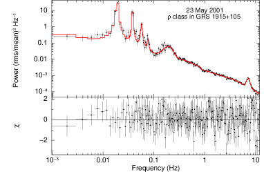
Figure 4: Power density spectrum shown for the “$\rho$” variability class observed on 23 May, 2001 (OBS-Id: 60405-01-02-00), fitted with Lorentians and broken power-law along with residuals.

For the above observation, we obtain the time averaged photon spectrum from standard2 data file of PCA. For data extraction, we use PCU2 only since it is reliably on throughout the observation and has the best calibration accuracy. Using PCA responses and latest background spectral file, the source spectrum in the energy range 3.0$-$25.0 keV is fitted with a two component model : multi-colour disk blackbody ($\tt diskbb$ in $\tt XSpec$) model and a simple power-law ($\tt powerlaw$ in $\tt XSpec$), along with a Gaussian component at $\sim$ 6.4 keV and all components are modified by Galactic absorption ($\tt TBabs$ in $\tt XSpec$). The fit gave a $\chi 2/dof=40.41/40$ and the best fit spectral parameters are listed in Table (1).

We calculate time-lag spectra using cross spectrum techniques (Nowak et al., 1999) in different energy bands in the range 3.20 $-$ 19.85 keV, where the reference band for lag calculation is chosen to be 3.69 $-$ 4.52 keV at both fundamental and harmonic frequencies. The rms was calculated by computing the power spectrum for different energy bins. Each power spectrum was fitted with a broken power-law and Lorentzians as shown in Fig. 4. Then by integrating the fitted components, the rms was calculated. Table (1) shows the values of the parameters used to model the observed lag and fractional rms. As can be seen in Fig.(5), the time-lag at fundamental (top left panel) shows a reversal around $\sim$ 12 keV while for the next harmonic (top right panel) the time-lag seems to rise at least up to $\sim$ 20 keV. However, the model-predicted spectrum fits the data well and the extension of the fitted model till 40 keV shows saturation around 25 keV. Because of poor coherence and poor statistics above 20 keV for RXTE/PCA, we are unable to verify the model-predicted saturation using actual data.

While a detailed analysis of the energy dependent rms and time-lag for different observations during the $\rho$ class variability will be presented elsewhere (Mir et. al. to be submitted), here we have used one observation as a typical example. We note that the qualitative behaviour of the energy dependence is fairly generic. Indeed, the detailed phase resolved spectroscopy of different observations also show that the energy dependence is similar despite changes in the frequency of the oscillations (Neilsen et al., 2011, 2012)

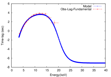
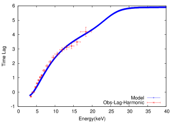
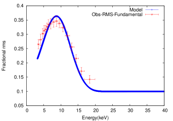
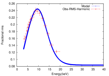
Figure 5: The observed and predicted energy dependent time-lag and rms at the fundamental (left panels) and for the next harmonic (right panels) observed on 23 May, 2001. The parameters used for the model are listed in Table 1. The four predicted curves are determined by only four free parameters

Table 1: Best fit parameters obtained from time-averaged spectrum fitting and from the proposed model fitting of the energy dependent time-lag and rms for the 23 May 2001 observation of GRS 1915+105 during the $\rho$ class

kTin	Nd	$\it p$	$N_{p}$	N
(keV)
1.47${}_{-0.01}^{+0.01}$	220${}_{-11.14}^{+11.10}$	2.85${}_{-0.02}^{+0.02}$	34${}_{-2.4}^{+2.3}$	3.15${}_{-.25}^{+.25}$
$\beta$	$\omega\tau_{d}$	$\Gamma$	$\delta\dot{M}$
0.73	2.25	0.1	0.47

Note: kT_in is the inner disk temperature (keV), ${\it p}$ is the photon power-law index, $N_{d}$ is the normalization of the disk blackbody component $N_{p}$ is the power-law component normalization and $N$ is obtained from the spectral information. $N$ is related to the ratio between the normalizations of power-law and disk blackbody (Appendix B). $\beta$ is the power-law variation of $R_{in}$ with $\dot{m}$ , $\omega t_{d}$ is the phase difference, $\Gamma$ is the dependence of power-law normalization on $\dot{m}$ and $\delta\dot{m}$ is the amplitude of the accretion rate variability.

3 Discussion and CONCLUSION

GRS 1915+105 shows a fascinating clockwork in its $\rho$-class, reflected in the highly periodic light curves which resemble closely to the human cardiogram, thus is also called as heartbeat state. We have studied the energy-dependent frequency resolved lags and fractional rms of this variability and they show a unique behaviour. With the lags of the order of few seconds, they cannot be attributed to light crossing time effects or due to Comptonization delays. The interesting feature is that the lag at the fundamental frequency show a phase reversal $\sim$ 10keV while at the next harmonic it keeps increasing with energy. The fractional rms amplitude at the fundamental and the next harmonic are also non-monotonic with energy.

We show, that these qualitative features can be explained in a model where the power-law component varies directly with the accretion rate while the inner disk radius responds after a time delay (DROID). Apart from parameters estimated from the time averaged spectrum, the energy dependent rms and time lag for the fundamental as well as the next harmonic are specified by only four free parameters and hence it is remarkable that such a simple picture can even qualitatively reproduce the overall features.

It should be emphasized that the analysis of energy dependent time-lag and rms and the model proposed to explain them are not different but complimentary to the phase resolved spectroscopy done earlier by Neilsen et al. (2011, 2012). Indeed as expected both analysis find that the basic feature of the oscillation is that the inner disk radius oscillates. The analysis done here provides another way of analyzing and understanding the data. Moreover, for observations of other types of oscillations, energy dependent rms and time-lag may be more easily estimated than performing a complete phase resolved spectroscopy.

A remarkable feature of this model is that the primary driver is a pure sinusoidal oscillation in the accretion rate and the other harmonics can be attributed to the non-linear relationship between the accretion rate and the inner disk radius as well as that between the two and the emergent spectrum. As the accretion rate increases the disk extends inwards, but this does not happen instantaneously. The inner disk responds after a time-delay that is found for this observation to be $\sim 20$ secs, which may be noted to be of the order of the viscous timescale. Thus our results present a scenario which has the potential to be developed into a physical interpretation based on the nature of the accretion disk instability.

The spectral components used in this model are simplistic. Instead of a power-law, the high energy component should be correctly modeled as a thermal Comptonization spectrum where the Comptonized flux should depend on the accretion rate. This will lead to variations in the spectral index which is considered in this work to be a constant. Moreover, there should also be a reflection component which may play an important part in the QPO formation (e.g. (Sobolewska & Życki, 2006)). The time-lag measured and modelled in this work is of the order of few seconds. Unless the reflector is significantly far away from the central object, any time-lag between the continuum and the reflection component (which is of the order sub-millisecs to few millisecs for a $\sim$ 10 $M_{\odot}$ black hole) can be neglected for the analysis done here. However, the rms spectra obtained from AGN (e.g., MCG 6$-$30$-$15) do show significant dip (Życki et al., 2010) at the position of 6.4 keV Fe emission line which is solely due to reflection. Therefore, instead of a powerlaw the combined continuum and reflection component needs to be considered, which will effect the results primarily in the Iron line region (Fabian et al., 2009). Such analysis would necessarily involve complex numerical computation which is presently out of scope of this work but can be considered as an extension of the present idea in future. It is likely that the deviation of the data from the predicted model, especially for the shape of the energy dependent rms curves, arises because of the simple spectral model used. A more realistic model would warrant fitting the data statistically and obtaining parameter values with confidence limits. It will be interesting to study how the parameters of the model change for different oscillations of the $\rho$ class, especially as a function of the frequency of the oscillations. Such a study will shed light on structural changes that occur during these oscillations and will help in obtaining a complete hydrodynamic understanding of the phenomenon.

Finally, the model maybe applicable to other QPOs observed in different systems where the disc component varies significantly during the oscillation. Observations of different black hole systems by the recently launched Indian multi-wavelength satellite ASTROSAT is expected to provide high quality event tagged data which would be ideally suited for such analysis.

4 ACKNOWLEDGEMENTS

MHM is highly thankful to IUCAA, Pune for allowing the periodic visit to the institute which has helped in carrying out this work and to UGC, New Delhi for granting the research fellowship.

Appendix A Accretion rate induced spectral variability of a disk and a power-law components

The accretion disk flux can be rewritten as

$$F_{D}\propto E^{-2/3}\dot{m}^{2/3}\int_{Z}^{\infty}\frac{y^{5/3}}{exp(y)-1}dy$$ (12)

where $Z\equiv E/kT_{in}$ and the relation $T_{in}\propto\dot{m}^{1/4}{r_{in}}^{-3/4}$ has been used. Its variation is given by

$$\delta F_{D} = (F_{D})_{\dot{m}}\delta{\dot{m}}+(F_{D})_{Z}\delta{Z}+\frac{1}{2}(F_{D})_{\dot{m}\dot{m}}\delta{\dot{m}^{2}}$$ (13)

$$+(F_{D})_{\dot{m}Z}\delta{\dot{m}}\delta{Z}+\frac{1}{2}(F_{D})_{ZZ}\delta{Z}^{2}$$

Here and as has been used in the main text, we denote the normalized variation $\delta X=\Delta X/X$ and define

$$(Z)_{X}=\frac{X}{Z}\frac{\partial Z}{\partial X}\;\;\;\;\hbox{and}\;\;\;\;(Z)_{XY}=\frac{XY}{Z}\frac{\partial}{\partial X}\frac{\partial Z}{\partial Y}$$ (14)

The derivatives can be computed to be $(F_{D})_{\dot{m}}=2/3$, $(F_{D})_{\dot{m}\dot{m}}=-2/9$,

$$(F_{D})_{Z}=f(Z)=\frac{Z^{\frac{8}{3}}}{({e^{Z}-1}){\int_{Z}^{\infty}\frac{y^{\frac{5}{3}}}{exp(y)-1}\,dy}}$$ (15)

$$(F_{D})_{ZZ}=f(Z)(\frac{5}{3}-k(Z))=f(Z)(\frac{5}{3}-\frac{ze^{Z}}{e^{Z}-1})$$ (16)

and $(F_{D})_{\dot{m}Z}=2f(Z)/3$.

Since Z depends on $T_{in}$ which in turn depends on $\dot{m}$ & $r_{in}$, as $Z=\alpha\dot{m}^{-1/4}r_{in}^{3/4}$, we have:

$$\delta Z=\frac{3}{4}\delta r_{{in}}-\frac{1}{4}\delta{\dot{m}}-\frac{3}{32}(\delta r_{{in}})^{2}+\frac{5}{32}(\delta\dot{m})^{2}-\frac{3}{16}\delta\dot{m}\delta r_{{in}}$$ (17)

The power-law component is assumed to depend on the accretion rate as $F_{p}\propto\dot{m}^{\Gamma}E^{-P}$ and hence

$$\delta F_{p}=\Gamma\delta\dot{m}+\frac{\Gamma(\Gamma-1)}{2}(\delta\dot{m})^{2}$$ (18)

The variation in the total flux $F_{t}=F_{D}+F_{p}$ is

$$\delta F_{t}=\frac{F_{D}}{F_{t}}\delta F_{D}+\frac{F_{p}}{F_{t}}\delta F_{p}$$ (19)

Next assuming that the inner disk radius follows the accretion rate with a time delay $r_{in}(t)\propto\dot{m}^{-\beta}(t-\tau_{d})$ and that the accretion rate undergoes a pure sinusoidal variation at an angular frequency $\omega$ i.e. $\delta\dot{m}=|\delta\dot{m}|e^{i\omega t}$ the inner disk variation is given by

$$\delta r_{in}=-\beta|\delta\dot{m}|e^{i\omega(t-\tau_{d})}+\frac{\beta(\beta+1)}{2}|\delta\dot{m}|^{2}e^{2i\omega(t-\tau_{d})}$$ (20)

Finally collecting terms proportional to $e^{i\omega t}$ and $e^{2i\omega t}$, we get for the fundamental oscillation,

$$\delta F_{t}^{f}=\frac{|\delta\dot{m}|}{1+\frac{F_{p}}{F_{d}}}\left(Ae^{i\omega t}+Be^{i\omega(t-\tau_{d})}\right)$$ (21)

and for the next harmonic:

$$\delta F_{t}^{h}=\frac{|\delta\dot{m}|^{2}}{1+\frac{F_{p}}{F_{d}}}\left(A^{\prime}e^{2i\omega t}+B^{\prime}e^{2i\omega(t-\tau_{d})}+C^{\prime}e^{2i\omega(t-\tau_{d}/2)}\right)$$ (22)

where

$$A=\frac{2}{3}+\frac{f(z)}{4}+\Gamma\frac{F_{p}}{F_{d}}$$

$$B=\frac{3}{4}\beta f(z)$$

$$A^{\prime}=-\frac{1}{9}+\frac{f(z)}{8}\left(\frac{k(z)}{4}-\frac{1}{3}\right)+\frac{1}{2}\Gamma(\Gamma-1)\frac{F_{p}}{F_{d}}$$

$$B^{\prime}=\frac{3}{8}f(z)\left(\beta^{2}\left(\frac{3}{4}k(z)-1\right)-\beta(\beta+1)\right)$$

$$C^{\prime}=\frac{3}{16}\beta k(z)f(z)$$

Appendix B Estimating the power-law to disk flux ratio from time-averaged spectrum

In terms of $Z=E/kT_{in}$, the ratio of the power-law to disk flux can be written as

$$\frac{F_{p}}{F_{d}}=NG(Z,p)=NZ^{-(p+2)}f(Z)(e^{Z}-1)$$ (23)

From Xspec model fitting of the spectrum we get the normalization of the power-law $F_{p}=N_{p}E^{-P}$ and that of the disk emission,

$$N_{d}=\left(\frac{(r_{in}/kms)}{(D/10kpc)}\right)^{2}cos(\theta)$$ (24)

By carefully comparing the flux equations, substituting $Z$ for $E$ and converting the energy unit from keV to ergs, one gets

$$N=\frac{3}{16\pi}\frac{N_{p}}{N_{d}}(kT_{in})^{-(p+2)}hc^{2}\left(\frac{10^{5}}{10kpc}\right)^{-2}\left(\frac{ergs}{keV}\right)^{-3}$$ (25)

or numerically

$$N\approx 1.316\times 10^{2}\times\frac{N_{p}}{N_{d}}\left(\frac{kT_{in}}{1keV}\right)^{-(p+2)}$$ (26)

References

- Axelsson, Done, & Hjalmarsdotter (2014) Axelsson M., Done C., Hjalmarsdotter L., 2014, MNRAS, 438, 657
- Belloni et al (1997) Belloni, T., Mendez, M., King, A. R., van der Klis, M. & van paradijs, J. 1997, ApJ, 488, L109
- Belloni et al (1997) Belloni, T., Mendez, M., King, A. R., van der Klis, M. & van paradijs, J. 1997, ApJ, 479, L145
- Belloni et al (2000) Belloni, T., Klein-Volt, M., Mendez, M., van der Klis, M. & van paradijs, J. 2000, A&A, 355, 271
- Fabian et al. (2009) Fabian, A. C., Zoghbi, A., Ross, R. R., et al. 2009, Nature, 459, 540
- Frank, King & Raine (2002) Frank, J., King, A. R., Raine, D. J., 2002, Accretion Power in Astrophysics , 3rd edn. Cambridge Univ. Press, Cambridge
- Ingram & van der Klis (2015) Ingram A., van der Klis M., 2015, MNRAS, 446, 3516
- Janiuk, Czerny, & Siemiginowska (2000) Janiuk A., Czerny B., Siemiginowska A., 2000, ApJ, 542, L33
- Janiuk & Czerny (2005) Januik, A., Czerny, B., 2005, MNRAS, 205, 356
- Kumar & Misra (2014) Kumar N., Misra R., 2014, MNRAS, 445, 2818
- Lee, Misra & Taam (2001) Lee, H. C., Misra, R., Taam, R. E., 2001, ApJ, 549, L229
- Lightman & Eardley (1974) Lightman, A. P., Eardley, D. M., 1974, ApJ, 187, L1
- Mirabel & Rodriguez (1994) Mirabel, I. F., Rodriguez, L. F., 1994, Nature, 371, 46
- Misra & Mondal (2013) Misra, R., Mondal, S., 2013, ApJ, 779, 71
- Morgan, Remillard & Greiner (1997) Morgan, E., Remillard, R. A., & Greiner, J., 1997, ApJ, 482, 993
- Muno, Morgan & Remillard (1997) Muno, M. P., Morgan, E. H., & Remillard, R. A , 1999, ApJ, 527, 321
- Nayakshin, Rappaport, & Melia (2000) Nayakshin S., Rappaport S., Melia F., 2000, ApJ, 535, 798
- Neilsen et al. (2011) Neilsen, J., Remillard, R., Lee, J. C., 2011, ApJ, 737, 69
- Neilsen et al. (2012) Neilsen, J., Remillard, R., Lee, J. C., 2012, ApJ, 750, 71
- Nowak et al. (1999) Nowak, M. A., Wilms, J., Dove, J. B., 1999, ApJ, 517, 355
- Pahari et al. (2013a) Pahari, M., Neilsen, J., Yadav, J. S., Misra, R., Uttley, P., 2013a, ApJ, 778, 136
- Pahari et al. (2013b) Pahari, M., Yadav, J. S., Rodriguez, J., Misra, R., et al., 2013b, ApJ, 778, 46
- Sobolewska & Życki (2006) Sobolewska, M. A., Życki, P. T., 2006, MNRAS, 370, 405
- Taam & Lin (1984) Taam, R. E., Lin, D.N. C., 1984, ApJ, 287, 761
- Taam, Chen & Swank (1997) Taam, R. E., Chin, X., Swank, J. H., 1997, ApJ, 485, L83
- Życki et al. (2010) Życki, T. P., Ebisawa, K., Niedzwiecki, A., Miyakawa, T., 2010, PASJ, 62, 1185