ON SPARSE RECONSTRUCTIONS IN NEAR-FIELD ACOUSTIC HOLOGRAPHY USING THE METHOD OF SUPERPOSITION

Abstract

The method of superposition is proposed in combination with a sparse $\ell_{1}$ optimisation algorithm with the aim of finding a sparse basis to accurately reconstruct the structural vibrations of a radiating object from a set of acoustic pressure values on a conformal surface in the near-field. The nature of the reconstructions generated by the method differs fundamentally from those generated via standard Tikhonov regularisation in terms of the level of sparsity in the distribution of charge strengths specifying the basis. In many cases, the $\ell_{1}$ optimisation leads to a solution basis whose size is only a small fraction of the total number of measured data points. The effects of changing the wavenumber, the internal source surface and the (noisy) acoustic pressure data in general will all be studied with reference to a numerical study on a cuboid of similar dimensions to a typical loudspeaker cabinet. The development of sparse and accurate reconstructions has a number of advantageous consequences including improved reconstructions from reduced data sets, the enhancement of numerical solution methods and wider applications in source identification problems.

1 Introduction

Near-field acoustic holography (NAH) was first documented in $1980$ [1, 2] as a method for reconstructing acoustic radiation from vibrating structures based on acoustic pressures measured in a hologram plane. This was originally carried out using Fourier acoustics and so was only suitable for geometries corresponding to the separable geometries of the acoustic wave equation such as an infinite plane, an infinite cylinder or a sphere in a free field. Recent progress [3] has seen ideas from signal processing and imaging, and in particular the much celebrated compressive sampling (or compressed sensing) [4], adopted to reduce measurement requirements and reconstruct acoustic fields above the Nyquist frequency. In this paper we develop a method based on an inverse formulation of the superposition method proposed by Koopman et al. [5] that can reconstruct acoustic fields from arbitrary shaped radiating objects and make use of sparse reconstruction principles as proposed in Ref. [3].

Near-field acoustic holography for arbitrary geometries was first performed using the inverse boundary element method (IBEM) [6]. A large number of publications on IBEM have since emerged, and more recently with the IBEM combined in hybrid methods which employ expansions of particular solutions of the Helmholtz equation to enrich the measured pressure data [7, 8]. One drawback of the IBEM is that it suffers from the same irregular frequency problem (at the resonances of the associated interior domain) as the forward boundary element method (BEM) [9]. Whilst this problem can be treated using the same methods as for the forward problem (for example, using the Burton and Miller method [10] as in Ref. [9], or the so-called combined Helmholtz integral equation formulation (CHIEF) [11]), such methods complicate the implementation and reduce the computational efficiency to some degree.

In addition to the irregular frequency problem, boundary element approaches also require very fine meshes to accurately represent solutions at high frequencies, and to give good representations of the acoustic field in the immediate vicinity of the radiating object. A number of methods have been suggested to resolve the shortcomings of IBEM in a manner that is both computationally efficient and relatively straightforward to implement. These methods effectively fit the measured pressure data to a linear combination of basis functions, and then use the coefficients determined through this approximation to determine the normal velocity of the vibrating object. The most well-known of these methods with respect to NAH are the Helmholtz equation least squares (HELS) method proposed by Sean Wu and co-workers [12, 13] and the method of superposition, which was applied to NAH in Refs. [14, 15], including a comparison against boundary element approaches in the latter case. For HELS, the basis functions are chosen as particular solutions to the Helmholtz equation on an idealised domain, typically a sphere. In the case of the superposition method then it is the free space Green’s functions that are employed for the basis.

It is shown in Ref. [5] that the superposition method for an exterior acoustic problem is equivalent to the Helmholtz integral equation. This is one reason for favoring the superposition approach to HELS, where the chosen basis is typically only complete outside the minimum sphere enclosing the radiating object [13]. This would be a drawback for approximating radiation from objects that are far from spherical in the region inside this minimum sphere. Koopman et al. [5] also argue that the superposition method will not suffer from the same irregular frequency problem as the boundary element method since the set of source points chosen for the superposition (after truncating the superposition integral to a finite sum) will not form a unique boundary surface inside the interior volume. However, the computations in Ref. [5] were only performed with small numbers of source points, and irregular frequency problems may arise should the source points more closely represent an interior boundary surface [16, 17].

One of the main challenges involved in the superposition method is obtaining an optimal choice of source (or charge) points over which to compute the superposition. In particular, research on (forward) interior Helmholtz problems [18] suggests that the source points should be chosen close to the radiating surface so that no singularities of the analytically continued solution lie between the charge points and the radiating surface. However, for the exterior problem, Koopman et al. [5] report that choosing the charge points too close to the radiating surface degrades the accuracy of the method, whilst choosing charge points too far from the surface leads to very poor conditioning. Applying the superposition method together with a nonlinear optimisation algorithm to optimise the accuracy of the solution over both the charge point strengths and locations is known as the method of fundamental solutions, see for example Refs. [19, 20]. We will show that in combination with sparse optimisation methods, a relatively small number of charge points can be chosen to accurately reconstruct the surface velocity, particularly in the sub-Nyquist frequency regime.

Regularisation schemes for NAH are typically based on standard Tikhonov methods, an excellent overview is presented in Ref. [21]. The most favorable method for selecting the regularisation parameter in NAH applications is reported as a modified generalised cross validation (GCV) method, although many other possibilities are discussed in Ref. [21]. Recent work [3] has suggested the possibility of using $\ell_{1}$ optimisation algorithms to instead in cases when a suitable dictionary of basis functions can be defined. Whilst this leads to a loss of efficiency in the optimisation process, it also promotes sparsity of the solution, and the convexity of the $\ell_{1}$ norm means that convex optimisation toolboxes such as SPGL1 [22] or CVX [23] can be applied. Chardon et al. [3] combine sparse optimisation techniques with a Fourier basis / plane wave approximation of the solution on flat star-like plates and report accurate reconstructions with sparse basis expansions. In combination with randomised measurement data, these methods gave faithful reconstructions, even above the Nyquist frequency. More recently, sparse $\ell_{1}$ optimisation with a plane wave basis has been proposed as a means of source identification from spherical acoustic radiators [24].

In this paper we discuss the possibility of a sparse solution representation using $\ell_{1}$ optimisation techniques based on the superposition method for application to general three dimensional problems. A study of this combination of methods for reconstructing vibration of flat plates has recently been presented in Ref. [25]. The method of superposition appears to be the most promising approach since there are close links between plane wave method and the method of superposition for bounded domains as described in Ref. [26]. In addition, the superposition method is typically accurate for frequencies above the six degrees of freedom per wavelength rule of thumb for boundary element methods [18] and can handle internal resonance frequencies in a relatively simple manner [16, 17]. The application and suitability of these methods will also be considered for the reconstruction of the Neumann boundary data on a cuboid of similar dimensions to a typical loudspeaker cabinet over a range of frequencies.

Initially we will study test problems where the exterior acoustic field is generated by a monopole point source inside the structure. In this case the solution could be represented exactly for arbitrarily high frequencies using the method of superposition if one of the points on the surface of interior charge points coincides with the monopole generating the acoustic field. However, in general such information would not be known a-priori when sampling an acoustic field in NAH. We will therefore examine the dependence of the reconstruction on the locations of the charge points and the monopole generating the acoustic field. Finally, we will consider a case where the acoustic field is not generated by an interior monopole, but rather by a relatively small vibrating patch on an otherwise rigid structure. This leads to a problem where the method of superposition should return a sparse expansion for interior charge point surfaces very close to the physical boundary, since the weighting of sources close to the vibrating region will be dominant compared to those close to the rigid part of the structure. The latter (locally radiating) case also has parallels with the situation that arises when modelling acoustic radiation from loudspeakers.

2 Method of Superposition for Near-field Acoustic Holography

Let $\Omega\subset\mathbb{R}^{3}$ be a finite domain with boundary surface $\Gamma$. Let $\Omega_{+}=\mathbb{R}^{3}\setminus\bar{\Omega}$ denote the unbounded exterior domain, which is assumed to be filled with a homogeneous compressible acoustic medium with density $\rho$ and speed of sound $c$. For a time-harmonic disturbance of frequency $\omega$, the sound pressure $p$ satisfies the homogeneous Helmholtz equation in $\Omega_{+}$

$$\Delta p+k^{2}p=0,$$ (1)

where $k=\omega/c$ is the wave-number. Since this work considers an unbounded exterior domain, then $p$ must also satisfy the Sommerfeld radiation condition. The superposition method approximates $p$ at some point $\mathbf{x}\in\bar{\Omega}_{+}$ using a basis expansion of the form

$$p(\mathbf{x})\approx\sum_{j=1}^{n}\sigma_{j}G_{k}(\mathbf{x},\mathbf{y}_{j}),$$ (2)

where $G_{k}$ is the free space Green’s function for Helmholtz equation in three dimensions given by

$$G_{k}(\mathbf{x},\mathbf{y})=\frac{e^{ik|\mathbf{x}-\mathbf{y}|}}{4\pi|\mathbf{x}-\mathbf{y}|}.$$ (3)

Here $\mathbf{y}_{i}\in\Omega$, $i=1,...,n$ are the source locations and $\sigma_{i}$ are the source strengths, which are determined by application of the method.

In the NAH problem we are given values of the acoustic pressure $p$ at a discrete set of points the acoustic near field within $\Omega_{+}$. We will assume that the data points $\mathbf{x}_{i}$, $i=1,...,m$ lie on a surface $\Gamma^{*}\subset\Omega_{+}$. Note that the pressure data is usually obtained from measurements using a microphone array. However, in this work we only generate the pressure data numerically as described in Section 4. The NAH problem is to use the given pressure data to recover the Neumann boundary data on $\Gamma$. Solving this problem via the method of superposition is then a matter of finding the set of source strengths $\sigma_{j}$, $j=1,...,n$, that reproduce the acoustic pressure data to some desired accuracy in the least squares sense. That is, $\sigma_{j}$ are chosen so that the $\ell_{2}$ norm of the residual vector $\mathbf{r}$, with entries given by

$$r_{i}=p(\mathbf{x}_{i})-\sum_{j=1}^{n}\sigma_{j}G_{k}(\mathbf{x}_{i},\mathbf{y}_{j})$$ (4)

for $i=1,..,m$, is smaller than a desired error tolerance. Once the source strengths have been obtained then the Neumann boundary data can be recovered from

$$\frac{\partial p}{\partial\mathbf{n}}(\mathbf{x})\approx\sum_{j=1}^{n}\sigma_{j}\frac{\partial G_{k}}{\partial\mathbf{n}}(\mathbf{x},\mathbf{y}_{j}),$$ (5)

where $\mathbf{n}$ is the outward unit normal to $\Gamma$. Note that the linearised Euler equation for time harmonic waves leads to the following simple relationship between the Neumann boundary data computed here, and the normal velocity $v$ of the radiating object

$$\frac{\partial p}{\partial\mathbf{n}}=i\omega\rho v.$$ (6)

Regularisation is always required in general, even for $n=m$, since NAH is an ill-posed inverse problem (see for example [9]). For experimental problems, the pressure measurements will contain errors and the ill-posedness of the problem means that these errors are amplified in the (unregularised) solutions, often rendering them meaningless. Most previous work on NAH has concentrated on using Tikhonov regularisation, together with generalised cross validation (GCV). In the next section we describe a scheme designed to promote sparsity in the solution as suggested in Ref. [3] for two-dimensional planar problems.

3 Regularisation and Sparse Reconstruction

One of the oldest and most widely used regularisation methods is Tikhonov regularisation, which applied to equation (4) leads to the following minimisation problem

$$\hat{\bm{\sigma}}=\mathrm{arg}\min_{\bm{\sigma}}\left\{\|\mathbf{r}\|_{2}^{2}+\lambda\|L\bm{\sigma}\|_{2}^{2}\right\},$$ (7)

where $L$ is the Tikhonov matrix (most simply chosen as the identity matrix) and $\lambda>0$ is a regularisation parameter to be determined. We have also introduced the notation $\bm{\sigma}=[\sigma_{1}\>\>\sigma_{2}\>\ldots\>\sigma_{n}\>]^{T}$ for the vector containing the source strengths, and likewise $\hat{\bm{\sigma}}$ is the vector containing the regularised and reconstructed source strengths at the $n$ interior source points.

In this work we adopt the alternative regularisation approach of Chardon et al. [3], which favors sparse representations of the solution. In other words, it (approximately) minimises $|\bm{\sigma}|_{0}$, the number of non-zero entries of $\bm{\sigma}$. As noted by Chardon et al. [3], the possibility of a sparse reconstruction is highly dependent on the basis functions used to represent the solution. In the superposition method, these basis functions are the fundamental solution of the Helmholtz equation at a set of distinct interior charge points. The results in Koopman et al. [5] suggest the feasibility of sparse solution representations for a large range of wavenumbers using the superposition method. The results presented in the next section will investigate the conditions whereby high quality sparse representations are indeed possible. For the examples considered here we expect that the quality of the solutions attainable will be highly dependent on the location of the interior charge points used for the superposition. The acoustic pressure data is created by either a single interior monopole, or by applying the BEM to give the acoustic field radiated from a relatively small vibrating patch. We will investigate whether the sparse reconstruction approach can pick out solutions $\bm{\sigma}$ that make use of the underlying sparsity in these examples, where this sparsity arises either due to the low number of monopoles needed to generate the field in the former case, or due to the relatively small region over which the reconstructed field is dominant in the latter case.

Directly minimising $|\bm{\sigma}|_{0}$ is often intractable due to non-convexity [3]. We therefore instead seek to minimise the $\ell_{1}$ norm

$$\|\bm{\sigma}\|_{1}=\sum_{j}|\sigma_{j}|.$$ (8)

The use of the $\ell_{1}$ norm allows one to apply powerful convex optimisation algorithms and still promotes sparsity by making many of the components of $\bm{\sigma}$ negligibly small, meaning that they can be well approximated by zero without degrading the reconstructed solution. The following procedure will be applied to find a sparse representation $\hat{\bm{\sigma}}$ of the source strengths $\bm{\sigma}$

$$\hat{\bm{\sigma}}=\mathrm{arg}\min_{\bm{\sigma}}\|\bm{\sigma}\|_{1}\>\>\>\mathrm{subject}\>\>\mathrm{to}\>\>\>\|\mathbf{r}\|_{2}^{2}\leq\epsilon.$$ (9)

This procedure will be implemented using the convex optimisation toolbox CVX [23]. This procedure requires a data fidelity constraint $\epsilon$ to be specified. Choosing this parameter involves a trade off between allowing sparser solutions with larger values of $\epsilon$ and achieving more accurately reconstructed solutions with smaller values of $\epsilon$. Chardon et al. [3] recommend a choice of $\epsilon$ of the order $20\%$ to $30\%$ of the $\ell_{2}$ norm of the measured pressure data. However, a good choice of $\epsilon$ is likely to depend on how noisy the pressure data is and hence will be problem dependent.

For completeness, and to emphasise the links between the $\ell_{1}$ regularisation approach and Tikhonov regularisation we note that (9) may be expressed in the form [3, 27]

$$\hat{\bm{\sigma}}=\mathrm{arg}\min_{\bm{\sigma}}\left\{\|\mathbf{r}\|_{2}^{2}+\lambda\|\bm{\sigma}\|_{1}\right\}.$$ (10)

This procedure is known as the Basis Pursuit Denoising (BPDN) and is introduced in Sect. 5.1 of Ref. [27], where the interested reader can find further details, including a discussion of suitable choices of $\lambda$ in the presence of standard Gaussian noise. Here we simply note the parallels between the expression (10) and equation (7), and in particular that one of the main differences is the norm employed in the final term. In particular, the $\ell_{1}$ norm replaces the square of the $\ell_{2}$ norm in the Tikhonov case, and it is this difference that promotes sparsity in the $\ell_{1}$ approach. The differences between these two approaches will be investigated numerically in the next section.

4 Numerical Results

Numerical results will be computed for acoustic radiation from a cuboid of similar dimensions to a typical loudspeaker cabinet ($0.28\mathrm{m}\times 0.28\mathrm{m}\times 0.42\mathrm{m}$). Although the method of superposition is a mesh free method, we will use a triangulation of the cuboid to generate the points at which the pressure data is computed, as well as the internal charge points and the points at which we reconstruct the solution on $\Gamma$. In particular, for a given triangulation of $\Gamma$ we reconstruct the Neumann boundary data at the centroid of each triangle and project (from each centroid) a distance $\delta$ along the normal vector to $\Gamma$ into $\Omega_{+}$ to obtain the points where the exterior pressure data is recorded. The internal charge points are positioned on a cuboid inside $\Omega$, which is just a scaled down version of $\Gamma$ with scaling factor $\alpha\in(0,1)$. For example, a value of $\alpha=0.5$ corresponds to a cuboid surface of internal charge points whose dimensions are exactly half those of $\Gamma$. Assuming that $\Omega$ is centred at the origin, we simply take a point $\mathbf{x}\in\Gamma$ and multiply by $\alpha$ to obtain the corresponding point $\mathbf{y}$ on the internal surface of charge points thus

$$\mathbf{y}=\alpha\mathbf{x}.$$ (11)

Initially we reconstruct the boundary data generated by a point source at $\mathbf{x}_{0}=(0,\>0,\>z_{0})\in\Omega$, where $\Omega$ is centred at the origin. The pressure data is therefore of the form

$$(\mathbf{p}_{0})_{j}=a\frac{e^{ik|\mathbf{x}_{0}-\mathbf{x}_{j}|}}{|\mathbf{x}_{0}-\mathbf{x}_{j}|},\hskip 28.45274ptj=1,...,m,$$ (12)

where $a\in\mathbb{C}$ is the strength of the source, which in these examples is arbitrarily taken to be $a=3-i$. The boundary data generated at $\mathbf{y}\in\Gamma$ may also be obtained for the case of a point source at $\mathbf{x}_{0}=(0,\>0,\>z_{0})$ by replacing $\mathbf{x}_{j}$ in (12) by $\mathbf{y}\in\Gamma$, differentiating in the direction of $\mathbf{n}_{y}$ and evaluating at the centroids of the triangulation $\mathbf{y}=\mathbf{y}_{j}$ for $j=1,...,m$ to give

$$(\mathbf{v})_{j}=a\left(\frac{\mathbf{n}_{y_{j}}\cdot(\mathbf{x}_{0}-\mathbf{y}_{j})}{|\mathbf{x}_{0}-\mathbf{y}_{j}|^{3}}(1-ik|\mathbf{x}_{0}-\mathbf{y}_{j}|)e^{ik|\mathbf{x}_{0}-\mathbf{y}_{j}|}\right),\hskip 28.45274ptj=1,...,m.$$ (13)

Using this calculation it is possible to verify the accuracy of the (Tikhonov or $\ell_{1}$) regularised approximate solutions with different wavenumbers and singularity point positions $z_{0}$. We will also investigate the behavior of the method at irregular frequencies of the volume enclosed by the interior charge points, and the dependence on the dimensions / location of the interior charge point surface controlled by the parameter $\alpha$.

Uniformly distributed and additive white noise will be applied to $\mathbf{p}_{0}$ in order to more closely replicate experimental observations. The use of Gaussian noise was also considered and, in general, led to slightly more accurate reconstructions than uniformly distributed noise. However, the quality of the reconstructions also fluctuated more widely when using different Gaussian noise vectors (of the same norm) than for uniformly distributed noise, and so we present the results for uniformly distributed noise since we believe they give a more indicative and repeatable measure of the performance of our reconstruction methods. We denote the added noise vector as $\mathbf{w}$ and specify the ratio

$$w=\frac{\|\mathbf{w}\|_{2}}{\|\mathbf{p}_{0}\|_{2}},$$ (14)

referring to $w$ as the level of added noise in the sequel. Note that $w$ is related to the standard signal to noise ratio (SNR) via $\mathrm{SNR}=w^{-2}$, or in decibels, $\mathrm{SNR}_{\mathrm{dB}}=10\log_{10}\left(w^{-2}\right)$.

Finally, we consider the case of reconstructing a locally vibrating structure, where only a small region of the structure is vibrating. Such an assumption is typical for the case of a loudspeaker and also allows us to study a case where the locations of any singularities of the continuation of the acoustic field into $\Omega$ are unknown, as is usually the case in practice. Here the acoustic pressure data will be generated using the boundary element method applied to the forward Neumann problem described earlier. Through this example we demonstrate the broader applicability of the sparse reconstruction algorithm, where the structure of the measured signal should have a sparse structure, but not necessarily the basis for the superposition method.

4.1 Comparison with Tikhonov regularisation

First consider the case $k=1$ and $z_{0}=0.05$, where the frequency is relatively low, is not close to an irregular frequency and $\mathbf{x}_{0}$ is relatively close to the origin and will lie inside the surface on which the interior charge points are located. Under such conditions the superposition method is expected to work well. Table 1 shows the $\ell_{2}$ percentage errors in the reconstructed Neumann boundary data for three different regularisation strategies and differing noise levels. The three solution strategies to be compared are (i) $\ell_{1}$ regularisation and taking the sum over all interior charge points, (ii) sparse $\ell_{1}$ regularisation where only contributions from dominant charge points are considered, and (iii) standard Tikhonov regularisation using Generalised Cross Validation (GCV) to determine the regularisation parameter. In the latter case the computations have been performed using Hansen’s extensive regularisation toolbox for Matlab [28]. In the case of the sparse reconstruction, the criteria used to determine whether the $j$th charge point is dominant is if

$$\log\left(\frac{|\sigma_{j}|}{\min_{i}|\sigma_{i}|}\right)>\beta\log\left(\frac{\max_{i}|\sigma_{i}|}{\min_{i}|\sigma_{i}|}\right).$$

We will use the notation $N^{*}(\beta)$ for the number of dominant charge points satisfying this condition, taking $\beta=0.5$ by default and so we denote $N^{*}=N^{*}(0.5)$. The $\ell_{2}$ percentage error in the reconstructed solution $\hat{\mathbf{v}}$ is calculated using

$$\frac{\|\hat{\mathbf{v}}-\mathbf{v}\|_{2}}{\|\mathbf{v}\|_{2}}\times 100\%.$$ (15)

The pressure data are specified at a distance $\delta=0.035$m from $\Gamma$ and the internal source surface is scaled down to have dimensions $\alpha=1/3$ the size of $\Gamma$. We note that these choices should lead to good results based on the fact that $\delta$ should be chosen small enough to capture evanescent contributions to the pressure field, but still large enough to be a practical distance for taking experimental measurements. For a further discussion on the role of evanescent wave contributions in superposition methods for NAH problems, the interested reader is referred to Sect. 5 of Ref. [15]. For the choice of the parameter $\alpha$ (11), Koopman et al. [5] suggest that too small a value will lead to severe ill conditioning as the charge points become very close together, but choosing too large a value of $\alpha$ will also give poor results. A choice in the range $\alpha\in(0.1,0.6)$ is advised in Ref. [5]. It is also beneficial for the charge point surface to enclose any singularities of the associated interior problem [18]. For these experiments the number of charge points, the number of measurement points and the number of points at which we reconstruct the solution are all equal to 576. This is achieved by triangulating the internal source surface in an identical way to $\Gamma$ and taking the charge points at the triangle centroids.

The results in Table 1 show that in the noise free case, the reconstruction errors for both the full $\ell_{1}$ method and Tikhonov regularisation are very small with Tikhonov reconstruction performing better. A sparse representation of the solution is not feasible here in general unless one of the charge points coincides with the monopole generating the acoustic field; the $\ell_{1}$ optimisation identifies a relatively large number $N^{*}=98$ of dominant sources and the error of the ‘sparse’ reconstruction increases significantly compared with the reconstruction using all $576$ source points. However, once noise is present in the pressure data then sparse representations of the solution can be obtained with a similar level of accuracy to the Tikhonov approach. The reason for this can be explained by considering how the data fidelity parameter $\epsilon$ is chosen in (9). In particular we take

$$\epsilon=(\max\{\epsilon_{\text{min}},w\})^{2}\|\mathbf{p}_{0}\|_{2}^{2},$$ (16)

where $w$ is the level of noise added to the pressure data as before. Recall that larger choices of $\epsilon$ permit sparser solution representations. However, it only makes sense to choose a larger $\epsilon$ for noisy data, otherwise it leads to less accurate reconstructions. The parameter $\epsilon_{\text{min}}\geq 0$ is included as a tolerance level that is used for the low or zero noise case. A relatively large choice of $\epsilon_{\text{min}}$ will lead to sparser reconstructions at the expense of accuracy, and the converse is true for small $\epsilon_{\text{min}}$. The results in this work have been obtained with $\epsilon_{\text{min}}=\textsc{1e-6}$.

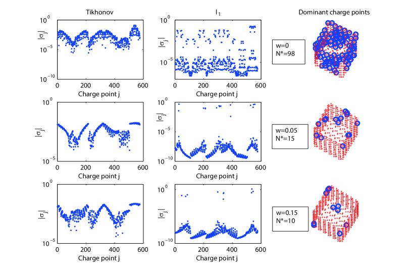
Figure 1: Left and centre columns: A comparison of the charge point strengths using both the Tikhonov and $\ell_{1}$ approaches for wavenumber $k=1$ and exterior pressure data generated by a point source at $(0,0,0.05)$. Right column: the locations of the dominant charge points for the $\ell_{1}$ approach. The top row shows the case of clean pressure data and the other rows show the results for differing levels of added noise $w$.

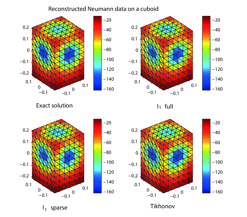
Figure 2: Neumann boundary data on a cuboid generated by a point source at $(0,0,0.05)$ with wavenumber $k=1$ and $15\%$ added noise. The plots compare the exact solution against those reconstructed using Tikhonov regularisation, the $\ell_{1}$ approach with all charge points and the sparse $\ell_{1}$ approach using only dominant charge points.

Figure 1 highlights the differing nature of the solutions reconstructed using the Tikhonov and $\ell_{1}$ approaches. The plots show that $\ell_{1}$ regularisation is more effective at promoting sparsity in the case of noisy data, and hence larger values of the data fidelity constraint $\epsilon$. In particular, when noise is added the solutions can be accurately reconstructed using only 10 to 15 of the 576 source points. This is further illustrated in Figure 2 which shows the reconstructed solution with noise level $w=0.15$ (or equivalently $\mathrm{SNR}_{\mathrm{dB}}=16.48\mathrm{dB}$) using each of the three solution strategies described above. The exact solution is also shown for reference.

In all three cases we achieve a faithful reconstruction of the Neumann data on the cuboid since the match to the exact solution is very good. Plots of the cases $w=0$ and $w=0.05$ are omitted for brevity, since as shown in Table 1, the reconstruction errors in these cases are even smaller and the likeness to the exact solution shown in Figure 2 would be even stronger. The main result of this section is that $\ell_{1}$ sparse regularisation can give similar accuracy to Tikhonov regularisation for noisy data, but with a small fraction of the number of charge points required to produce the reconstruction.

4.2 Higher and irregular frequencies

We now investigate the behavior of the method for some potentially problematic choices of the wavenumber $k$. First we look at the case when the frequency is increased, including when the Nyquist frequency is exceeded. Since our measurements are taken at triangle centroids then the resulting measurement grid is irregular and so the Nyquist frequency is not well-defined. We therefore choose the Nyquist frequency associated with the regular grid given by the triangle vertices, as a value approximately representative of the Nyquist frequency. For the discretisation considered in the previous section with $576$ triangles, the grid spacing is $\Delta x=0.04667$, meaning that the wavenumber corresponding to the Nyquist frequency is $k_{\mathrm{nyq}}=\pi/\Delta x=67.32$. We also investigate the performance of the method close to other typical threshold frequencies for numerical solution approaches, such as the six grid points per wavelength rule of thumb for finite and boundary element methods, which gives a maximum wavenumber of $k=22.44$ for the grid described above. The performance of the method at irregular frequencies will also be investigated. For the method of superposition these irregular frequencies are the resonances of the region enclosed by the interior source surface [5]. Numerical studies indicate that one such frequency is close to $k^{*}=17.54/\alpha$, which here is $k=52.62$.

Table 2 gives the reconstruction error for a range of wavenumbers $k$ using $\ell_{1}$ reconstruction techniques and compares the accuracy of the reconstruction using all 576 charge points, and using two different values of the sparsity parameter $\beta$. In particular, we compare the default choice used in the last section of $\beta=0.5$ with the choice $\beta=0.9$, which uses fewer charge points but at the potential cost of poorer accuracy. The maximum wavenumber studied corresponds to the wavelength being close to (but still greater than) the exterior measurement distance $\delta$. The results show that both irregular and high frequencies lead to a degradation in the accuracy of the reconstruction, and lead to a loss of sparsity in the reconstructions. Accurate and reasonably sparse reconstructions can be generated provided there are at least 3 data points per wavelength since for up to $k=44.88$ we can reconstruct the solution with a smaller error than the level of added noise ($15\%$) and with at least an order of magnitude reduction from the total number of charge points (576). These results are consistent with the findings of Ref. [18], where it is also suggested that a superposition method will give accurate results provided there are at least 3 degrees of freedom per wavelength. We note that if the surface of interior charge points includes the monopole generating the acoustic field then one would obtain exact representations for arbitrarily high frequencies.

In addition to the general trend of increased errors for higher frequencies, one also observes a local peak in the error at the characteristic wavenumber $k=52.62$. Here we see that the error is particularly poor for the sparse reconstruction with $\beta=0.9$, and that there is also a local peak in the number of dominant charge points. This suggests that sparse reconstructions are not feasible at higher frequencies or at irregular frequencies. However, the reconstruction error is lower than the noise level for the schemes using all charge points or with $\beta=0.5$ for all frequencies tested up to twice the Nyquist frequency. The results of this section therefore suggest that the method of superposition with $\ell_{1}$ regularisation can provide excellent reconstructions for frequencies up to around twice the Nyquist frequency, and that sparse reconstructions are feasible provided we have at least three data points per wavelength. Irregular frequencies degrade both accuracy and sparsity. However, if a more accurate and sparsely reconstructed solution was required at $k=52.62$, then we could change the scaling of the internal source surface (i.e. change $\alpha$) which would move the location of the irregular frequency. Changing $\alpha$ from $1/3$ to $0.4$ leads to a percentage error of 6.131% for both the full reconstruction and the sparse scheme with $\beta=0.5$, which identifies $N^{*}(0.5)=102$ dominant charge points. For $\beta=0.9$, the error increases to 16.00% with $N^{*}(0.9)=63$. Note that these results are far more consistent with the other results shown in Table 2 and the removal of the local error peaks is shown more clearly in Fig. 3, where the diamond symbols show the values computed with $\alpha=0.4$.

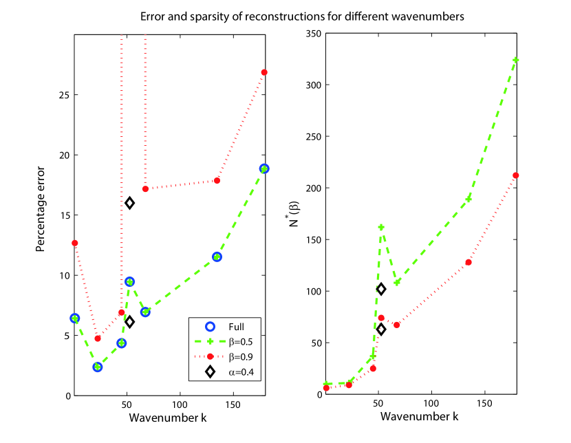
Figure 3: The accuracy and sparsity of the reconstructed solutions with $15\%$ added noise, $\alpha=1/3$ and $z_{0}=0.05$. The plots show the effect of changing the wavenumber $k$, including the effect of irregular frequencies and values above the Nyquist frequency.

The results presented by Chardon et. al. [3] using sparse plane wave reconstructions indicate that randomising the exterior data point locations (measurement locations) within the hologram plane facilitates sparse reconstructions above the Nyquist limit. Unfortunately, the reconstructed solutions using the method of superposition lose their sparsity at frequencies around and above the Nyquist limit and randomising the data point locations has been observed to degrade the accuracy of the reconstructed solution in general across the range of wavenumbers studied in Fig. 3. These observations are consistent with the findings in Ref. [29]. The main result of this section is that although in certain special cases $\ell_{1}$ sparse regularisation could give exact representations up to arbitrarily high frequencies, in general the reconstruction accuracy will decrease at higher frequencies. Irregular frequencies can also be treated simply by perturbing the surface of interior charge points.

4.3 Dependance on the singularity and charge point locations

The results in the previous sections all reconstructed the Neumann data generated from a point source located on the $z-$axis at $z_{0}=0.05$. This ensured that the singularity in the solution of the related interior problem was located within the interior charge point surface for $\alpha=1/3$. We now consider how the accuracy and sparsity of our reconstructed solutions depends on both the position of an interior source point generating the exterior pressure data, and the relative size/ position of the internal charge point surface controlled by the parameter $\alpha$ as described in Eq. (11).

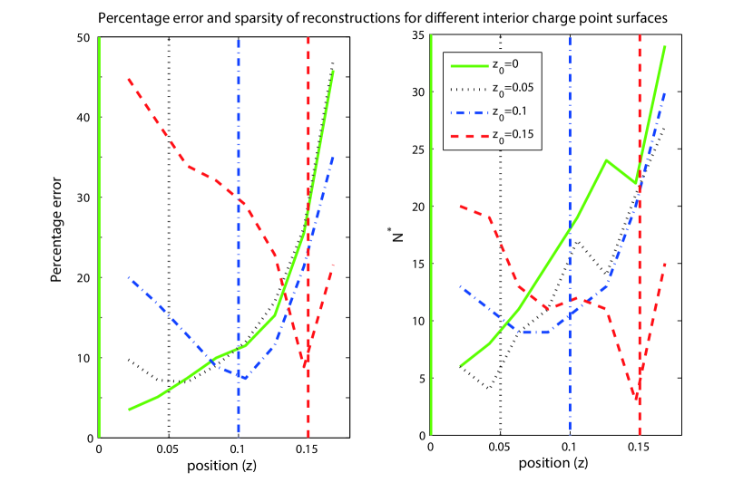
Figure 4: The accuracy and sparsity of the reconstructed solutions with $k=1$ and $15\%$ added noise. The plots show the effect of using a range of different sized interior charge point surfaces and different positions for the source point generating the boundary data.

Fig. 4 shows both the percentage errors for the sparse reconstructions and the value of the sparsity parameter $N^{*}(0.5)$ for different sized interior charge point surfaces and for different positions of the point source generating the exterior data. These quantities have been computed for values of $\alpha$ between $0.1$ and $0.8$, and for $z_{0}$ between $z_{0}=0$ and $z_{0}=0.15$. Instead of showing values of the parameter $\alpha$, Fig. 4 shows the corresponding $z-$coordinate where the interior charge point surface intersects the positive $z-$axis. In this way we are able to indicate the size of the interior charge point surface relative to the location of $z_{0}$ on the same axes. Note that since $\Gamma$ intersects the positive $z$-axis at $z=0.21$ (it is centred at the origin with total height $0.42$m), then the internal source surface with, for example, $\alpha=0.5$ will intersect the positive $z$-axis at $z=0.105$, and this is the value used along the horizontal axis in Fig. 4. In all cases the added noise level is $15\%$. Note that the relative errors obtained when reconstructing the solution using all charge points differs from that given by the sparse reconstruction by less than $1\%$.

Each subplot of Fig. 4 shows four curves, corresponding to each of four choices of $z_{0}$, and four vertical lines indicating the positions of the corresponding point $z_{0}$. The left subplot shows the percentage errors for different choices of interior source surface. We notice that the errors are minimised when the size of the interior source surface is such that it intersects the positive $z-$axis close to $z=z_{0}$, where the curve crosses its corresponding vertical line. Likewise, this right subplot shows that the number of charge points $N^{*}$ needed to obtain a sparse reconstruction is also minimal when the size of the interior source surface is such that it intersects the positive $z-$axis close to $z=z_{0}$. In general, the solutions are reasonably accurate for source surfaces intersecting the positive $z-$axis between $z=0.05$ and $z=0.1$, corresponding to choosing $\alpha=0.3$ or $\alpha=0.4$. Choosing $\alpha=0.8$ so that the source surface intersects the positive $z-$axis at $z=0.168$ gave the worst results in general. Interestingly, the results of this section suggest that it doesn’t seem to be critical whether or not the surface of interior charge points encloses any singularities in the modelled wave field. Furthermore, the results also point to important potential applications of the sparse superposition method developed in this work for source identification problems in general.

The main result of this section is that both the accuracy and sparsity of the reconstructed solution is enhanced when the surface of interior charge points includes points close to the location of the interior monopole generating the acoustic field. A major strength of the sparse reconstruction approach described here will therefore be in its application to source identification problems.

4.4 Example of a locally radiating structure

In this section we consider the problem of reconstructing the vibrations of a structure which is rigid, except over a relatively small region. This is both a typical assumption for applications to loudspeakers, and is also typical of problems commonly modelled using the method of patch NAH, whereby measurements and reconstructions only take place in the vicinity of the vibrating region (see for example Refs. [14, 30]). In the present study we use such an example for verification of the sparse superposition method for a problem where the pressure data is not generated by a monopole point source, and hence an optimal choice for the surface of internal charge points would not be related to the location of such a monopole.

We consider reconstructing Neumann boundary data given by a raised cosine function

$$\frac{\partial p}{\partial\mathbf{n}_{x}}(\mathbf{x})=\frac{1}{2}\left(1+\cos(10\pi|\mathbf{x}-\mathbf{x}_{0}|))\right),$$ (17)

inside the circle defined by $\Gamma\cap\{\mathbf{x}:10|\mathbf{x}-\mathbf{x}_{0}|<1\}$, with $\mathbf{x}_{0}=(0.14,0,-0.0525)$. Outside of this circle we let the Neumann boundary data be zero. The exterior pressure data at a distance $\delta=0.035$m from $\Gamma$ are generated using a Burton-Miller based BEM as described in Ref. [31] for example. The triangulation has been refined compared to the results in previous sections and now has $1024$ triangles / interior source points and $1024$ exterior data points. This has been done to improve the resolution of both the boundary data representation and the BEM approximation of the exterior pressure data. Note that here there is an extra source of noise (in addition to the $15\%$ added noise) in the acoustic pressure data due to the numerical error in the BEM approximation. The results of the sparse reconstruction technique for wavenumber $k=1$ are shown in Fig. 5. We found that a value of $\alpha$ between $0.3$ and $0.4$ gave the best results, which is consistent with the previous section, and hence we have taken $\alpha=1/3$.

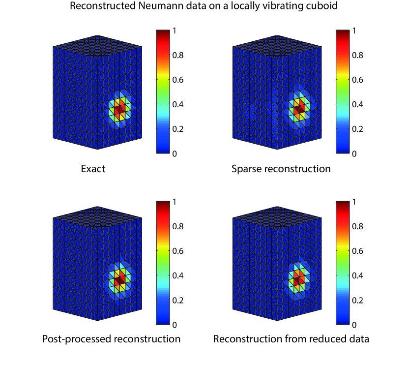
Figure 5: The Neumann boundary data for a locally radiating structure with $1024$ charge points, $1024$ data points, $k=1$ and $\alpha=1/3$. Comparison of the exact solution (upper left) with the sparsely reconstructed boundary data (upper right), the sparsely reconstructed boundary data after post-processing (lower left) and a reconstruction using only 28 charge points and a reduced data set with 800 values (lower right).

The upper subplots of Fig. 5 show that the sparse superposition method produces a good reconstruction of the vibrating region for the prescribed locally vibrating boundary data. The computations shown use $\beta=0.5$ to generate the sparse scheme leading to $N^{*}=30$ dominant charge points (of $1024$ in total). The percentage error in the sparse reconstruction is 21.19%, which is the same (up to the quoted level of accuracy) as the error using all $1024$ charge points for the reconstruction. We note that the boundary data to be reconstructed has $52$ out of $1024$ entries that are non-zero. Relatively significant errors arise in the quiet regions of the locally vibrating object, close to the edges of the cuboid that are nearest the vibrating region. If we assume prior knowledge of the non-vibrating regions and consider only the accuracy of the reconstruction over the vibrating region, then the error reduces to 9.843% for both the sparse and full data reconstructions. A plot of this post-processed result is shown in the lower left subplot of Fig. 5.

The lower right subplot of Fig. 5 shows the result of reconstructing the Neumann boundary data starting only with the $30$ dominant source points identified by the sparse reconstruction method and using a reduced data set sampled from the full data set at $800$ randomly selected points. The same post-processing procedure as described above has been applied to fix the solution in the non-vibrating regions to zero. The results shown are computed using Tikhonov regularisation (with only the 30 charge points identified by the initial sparse reconstruction), which gave slightly better accuracy than using the sparse reconstruction algorithm for a second time. The percentage error in the plotted reconstruction is 18.89%, compared with 26.36% for the reconstruction without post-processing. Using the sparse algorithm to reconstruct the solution instead gave errors around $3\%$ higher in each case. Note that these results all show an improvement on the reconstruction obtained from the same reduced acoustic data set, but using a basis with all $1024$ charge points. In this case the percentage error was more than doubled to 58.87%, and improved to 46.52% after post-processing. We remark that the reconstruction using the full basis with reduced data is an under-determined problem (the acoustic data are fewer than the number of unknowns), whereas the reconstruction from the sparse basis is over-determined. This suggests that reducing the number of charge points and changing the under-determined problem into an over-determined one is an important step for the efficient implementation of NAH with reduced data using the method of superposition. The main result of this section is that sparse reconstruction methods can still be applied when a suitable choice of dictionary of basis functions for the sparse reconstruction is not obvious, provided there is some inherent sparsity that can be exploited. Sparse reconstructions can also be used in conjunction with reduced acoustic field data sets giving reasonable results. In particular, the sparse basis representation leads to better accuracy and more efficient calculations than using the full basis with the reduced data set.

5 Conclusions

The method of superposition has been combined with a sparse $\ell_{1}$ reconstruction algorithm and applied to the problem of near-field acoustic holography. The developed sparse superposition method is able to reconstruct the normal velocity of a vibrating object using only a very small number of charge points in many cases, in contrast with a standard Tikhonov reconstruction. In particular, it appears that competitive sparse reconstructions can be generated provided the wavenumber is not too large and that the data can be assumed to be sufficiently noisy to permit a data fidelity parameter of at least $5\%$ of the size of the $\ell_{2}$ norm of the exterior pressure data. Sparsity also appears to be an important factor when considering reduced acoustic field data sets, where reconstructions using a sparse basis gave a considerable improvement in accuracy over using the full basis with all charge points. The results of the simulations point to a number of important future developments. The sparse superposition method could be used to generate initial conditions for the method of fundamental solutions, whereby the accuracy of the reconstruction is optimised over both the charge point strengths and locations using a non-linear optimisation algorithm. This technique could also be applied more widely to source identification problems, as the results have shown that when the charge points are close to point sources generating the exterior pressure data then the reconstruction becomes very sparse, and the charge points close to the generating point source are highly dominant.

Table 1: The $\ell_{2}$ percentage error in the reconstructed Neumann boundary data generated from a source point on the $z-$axis at $z_{0}=0.05$ with added noise and $k=1$.

Noise level $(\%)$	% error for $\ell_{1}$ full	% error for $\ell_{1}$ sparse	% error for Tikhonov
0	6.2091e-3	0.1097	1.009e-7
5	3.850	3.850	3.549
15	6.428	6.429	6.017

Table 2: The $\ell_{2}$ percentage error in the reconstructed Neumann boundary data generated from a source point on the $z-$axis at $z_{0}=0.05$, with internal source surface at $\alpha=1/3$ and $15\%$ added noise over a range of wavenumbers $k$.

$k$	% error: full	% error: $\beta=0.5$	$N^{*}(0.5)$	% error: $\beta=0.9$	$N^{*}(0.9)$
1	6.428	6.429	10	12.27	6
22.44	2.369	2.369	11	4.752	9
44.88	4.358	4.358	37	6.904	25
52.62	9.458	9.462	162	4797	74
67.32	6.937	6.937	108	17.18	67
134.6	11.15	11.15	189	17.86	128
179	18.89	18.89	324	26.87	212

References

- [1] E.G. Williams and J.D. Maynard, Holographic imaging without the wavelength resolution limit, Phys. Rev. Lett. 45 (1980) 554.
- [2] E.G. Williams, J.D. Maynard and E. Skudrzky, Sound source reconstructions using a microphone array, J. Acoust. Soc. Amer. 68 (1980) 340.
- [3] G. Chardon, L. Daudet, A. Peillot, F. Ollivier, N. Bertin and R. Gribonval, Nearfield acoustic holography using sparsity and compressive sampling principles, J. Acoust. Soc. Amer. 132(2) (2012) 1521.
- [4] E.J. Candès and M.B. Wakin, An introduction to compressive sampling, IEEE Sig. Proc. Mag. 25(2) (2008) 21.
- [5] G.H. Koopmann, L. Song, J. B. Fahnline, A method for computing acoustic fields based on the principle of wave superposition, J. Acoust. Soc. Amer. 86(6) (1989) 2433.
- [6] B.K. Gardner and R.J. Bernhard, A noise source identification technique using an inverse Helmholtz integral equation method, ASME J. Vib., Acoust., Stress, Reliab. Des. 110, (1988) 84.
- [7] S.F. Wu and X.Zhao, Combined Helmholtz equation-least squares method for reconstructing acoustic radiation from arbitrary shaped objects, J. Acoust. Soc. Amer. 112(1) (2002) 179.
- [8] S.F. Wu, Hybrid near-field acoustic holography, J. Acoust. Soc. Amer. 115(1) (2004) 207.
- [9] D.J. Chappell and P.J. Harris, A Burton-Miller inverse boundary element method for nearfield acoustic holography, J. Acoust. Soc. Amer. 126(1), (2009) 149.
- [10] A.J. Burton and G.F. Miller, The application of integral equation methods to the numerical solution of some exterior boundary-value problems, Proc. Roy. Soc. London, Ser. A. 323 (1971) 201.
- [11] H.A. Schenck, Improved integral equation formulations for acoustic radiation problems, J. Acoust. Soc. Amer. 44(1) (1968) 41.
- [12] Z. Wang and S.F. Wu, Helmholtz Equation-Least Squares (HELS) method for reconstructing the acoustic pressure field, J. Acoust. Soc. Amer. 102(4) (1997) 2020.
- [13] S.F. Wu, On the reconstruction of acoustic pressure fields usingthe Helmholtz equation least squares method, J. Acoust. Soc. Amer. 107(5) (2000) 2511).
- [14] A. Sarkissian, Method of superposition applied to patch near-field acoustic holography, J. Acoust. Soc. Amer. 118(2) (2005) 671.
- [15] N.P. Valdivia and E.G. Williams, Study of the comparison of the methods of equivalent sources and boundary element methods for near-field acoustic holography, J. Acoust. Soc. Amer. 120(6) (2006) 3694.
- [16] W. Benthien, and A. Schenck, Nonexistence and nonuniqueness problems associated with integral equation methods in acoustics, Computers and Structures, 65(3) (1997) 295.
- [17] A. Leblanc, R.K. Ing and A. Lavie, A wave superposition method based on monopole sources with unique solution for all wave numbers, Acta Acustica united with Acustica, 96(1), (2010) 125.
- [18] A.H. Barnett and T. Betcke, Stability and convergence of the Method of Fundamental Solutions for Helmholtz problems on analytic domains, J. Comput. Phys. 227(14) (2008) 7003.
- [19] G. Fairweather and A. Karageorghis, The method of fundamental solutions for elliptic boundary value problems, Adv.Comp. Math. 9(1-2) (1998) 69.
- [20] G. Fairweather, A. Karageorghis and P.A. Martin, The method of fundamental solutions for scattering and radiation problems, Eng. Anal. Boundary Elem. 27(7) (2003) 759.
- [21] E.G. Williams, Regularization methods for near-field acoustical holography, J. Acoust. Soc. Amer. 110(4), (2001) 1976.
-
[22]
E. van den Berg and M. P. Friedlander, SPGL1: A solver for
large-scale sparse reconstruction version 1.9, (2015),
https://www.math.ucdavis.edu/~mpf/spgl1/, last visited 06/02/2015. -
[23]
M. Grant and S. Boyd, CVX: Matlab software for disciplined convex
programming, version 2.1, (2015),
http://cvxr.com/cvx, last visited 06/02/2015. - [24] E. Fernandez-Grande and A. Xenaki, Sparse acoustic imaging with a spherical array. In Proc. Euronoise 2015, Maastricht, Netherlands, (2015).
- [25] E. Fernandez-Grande and A. Xenaki, The equivalent source method as a sparse signal reconstruction. In Proc. Internoise 2015, San Francisco, USA, (2015).
- [26] C.J.S. Alves and S.S. Valtchev, Numerical comparison of two meshfree methods for acoustic wave scattering, Eng. Anal. Boundary Elem. 29(4) (2005) 371.
- [27] S.S. Chen, D.L. Donoho, and M.A. Saunders, Atomic Decomposition by Basis Pursuit, SIAM J. Sci. Comp. 20, (1999) 33.
- [28] P.C. Hansen, Regularization Tools Version 4.0 for Matlab 7.3, Numerical Algorithms, 46 (2007) 189.
- [29] M. R. Bai, J.-H. Lin, and K.-L. Liu, Optimized microphone deployment for near-field acoustic holography: To be, or not to be random, that is the question, J. Sound Vib. 329(14) (2010) 2809.
- [30] E.G. Williams, Continuation of acoustic near-fields, J. Acoust. Soc. Amer. 113(3) (2003) 1273.
- [31] S. Amini, P.J. Harris and D.T. Wilton, Coupled Boundary and Finite Element Methods for the Solution of the Dynamic Fluid-Structure Interaction Problem, (Lecture Notes in Engineering Vol. 77, Springer-Verlag, Berlin, 1992).