Weyl, Dirac and Maxwell Quantum Cellular Automata:
analitical solutions and phenomenological predictions of the Quantum Cellular Automata Theory of Free Fields

Abstract

Recent advances on quantum foundations achieved the derivation of free quantum field theory from general principles, without referring to mechanical notions and relativistic invariance. From the aforementioned principles a quantum cellular automata (QCA) theory follows, whose relativistic limit of small wave-vector provides the free dynamics of quantum field theory. The QCA theory can be regarded as an extended quantum field theory that describes in a unified way all scales ranging from an hypothetical discrete Planck scale up to the usual Fermi scale.

The present paper reviews the elementary automaton theory for the Weyl field, and the composite automata for Dirac and Maxwell fields. We then give a simple analysis of the dynamics in the momentum space in terms of a dispersive differential equation for narrowband wave-packets, and some account on the position space description in terms of a discrete path-integral approach. We then review the phenomenology of the free-field automaton and consider possible visible effects arising from the discreteness of the framework. We conclude introducing the consequences of the automaton distorted dispersion relation, leading to a deformed Lorentz covariance and to possible effects on the thermodynamics of ideal gases.

I Introduction

The notion of cellular automaton was introduced by J. von Neumann in his seminal paper von Neumann (1966) where he aimed at modeling a self-reproducing entity. The idea behind the concept of a cellular automaton is that the richness of states exhibited by the evolution of a macroscopic system could emerge from a simple local interaction rule among its elementary constituents. More precisely, a cellular automaton is a lattice of cells that can be in a finite number of states, together with a rule for the update of cell states from time $t$ to time $t+1$. The principal requirement for such rule is locality: The state of the cell $\mathbf{x}$ at step $t+1$ depends on the states of a finite number of neighboring cells at step $t$. The use of classical cellular automata for simulation of quantum mechanics was proposed by ’tHooft Hooft (2014), followed by other authors Elze (2014).

The first author to suggest the introduction of the quantum version of cellular automata was R. Feynman in the celebrated paper of Ref. Feynman (1982). Since then, the interest in quantum cellular automata (QCAs), has been rapidly growing, especially in the Quantum Information community, leading to many results about their general structure (see e.g Refs.Schumacher and Werner (2004); Arrighi et al. (2011); Gross et al. (2012) and references therein). Special attention is devoted in the literature to QCAs with linear evolution, known as Quantum Walks (QWs) Grossing and Zeilinger (1988); Aharonov et al. (1993); Ambainis et al. (2001); Reitzner et al. (2011), which were especially applied in the design of quantum algorithms Childs et al. (2003); Ambainis (2007); Magniez et al. (2007); Farhi et al. (2007), providing a speedup for relevant computational problems.

More recently QCAs have been considered as a new mathematical framework for Quantum Field Theory D’Ariano (2010, 2011); Bisio et al. (2015b); D’Ariano and Perinotti (2014); Bisio et al. (2014); Arrighi et al. (2014); Arrighi and Facchini (2013); Farrelly and Short (2014, 2013). Within this approach, each cell of the lattice corresponds to the evaluation $\psi(\mathbf{x})$ of a quantum field at the site $\mathbf{x}$ of a lattice, with the dynamics updated in discrete time steps by a local unitary evolution. Assuming that the lattice spacing corresponds to an hypothetical discrete Planck scale, the usual quantum field evolution should emerge as a large scale approximation of the automaton dynamics. On the other hand, the QCA dynamics will exhibit a different behaviour at a very small scale, corresponding to ultra-relativistic wave-vectors.

The analysis of this new phenomenology is of crucial importance in providing the first step towards an experimental test of the theory as well as a valuable insight on the distinctive features of the QCA theory. Until now the research was mainly focused on linear QCAs which describe the dynamics of free field. By means of a Fourier transform the linear dynamics can be easily integrated and then, as we will show in section III.1, an approximated model for the evolution of particle states (i.e. state of the dynamics narrow-band in wave-vector) can be obtained. Moreover, it is also possible to derive an analytical solution of the evolution in terms of a path sum in the position space, thus giving the QCA analog of the Feynman propagator D’Ariano et al. (2014a, b). In section IV we will exploit these tools to explore many dynamical features of the QCA models for the Weyl and Dirac fields and to compare them with the corresponding counterpart emerging from the Weyl and Dirac Equation. We will see that, when considering massive Fermionic fields (e.g electrons) the deviations from the usual field dynamics cannot be reached by present day experiments, contrarily to the case of the QCA theory of the free electromagnetic field. In section IV.4 we will review the main phenomenological aspects of the QCA model for free photons (that in this framework become composite particles) with special emphasis of the emergence of a frequency-dependent speed of light, a Planck-scale effect already considered by other authors in the Quantum Gravity community Ellis et al. (1992); Lukierski et al. (1995); ’t Hooft (1996); Amelino-Camelia (2001); Magueijo and Smolin (2002). In the final Section of this paper we address two issues of the QCA theory that are still under investigation. The first one concerns the notion of Lorentz covariance: Because of its intrinsic discreteness, a QCA model cannot enjoy a notion of Lorentzian space-time and the usual Lorentz covariance must break down at very small distances. One way of addressing the problem of changing the reference frame is to assume that every inertial observer must observe the same dynamics. Then one can look for a set of modified Lorentz transformtion which keep the QCA dispersion relation invariant. The first step of this analysis are reported in Section V.1. The second issue we will briefly address in Section V.2 are thermodynamical effects that could emerge from modified QCA dynamics.

II Weyl, Dirac and Maxwell automata

A Quantum Cellular Automaton (QCA) describes the discrete time evolution of a set of cells, each one containing an array of quantum modes. In this section we review the QCA models for the free fermions and for the free electromagnetic field. For a complete presentation of these results we refer to Refs. Bisio et al. (2015b); D’Ariano and Perinotti (2014); Bisio et al. (2014). Within our framework we will consider Fermionic fields, our choice being motivated by the requirement that amount of information in finite number of cells must be finite. Then, each cell $\mathbf{x}$ of the lattice is associated with the Fermionic algebra generated by the field operators $\{\psi(\mathbf{x}),\psi^{{\dagger}}(\mathbf{x})\}$ which obey the canonical anticommutation relation $[\psi(\mathbf{x}),\psi^{{\dagger}}(\mathbf{x}^{\prime})]_{+}=\delta_{\mathbf{x},\mathbf{x}^{\prime}}$ and $[\psi(\mathbf{x}),\psi(\mathbf{x}^{\prime})]_{+}=0$ . With a slight genealization, we consider the case in which each cell correspond to more than one Fermionic mode. Different Fermionic modes will be denoted by an additional label, e.g. $\psi_{i}(\mathbf{x})$. The automaton evolution will be specified by providing the unit-step update of the Fermionic field operators. This rule defines the primitive physical law, and must then be as simple and universal as possible. This principle translates into a minimization of the amount of mathematical parameters specifying the evolution. In particular we constrain the automaton to describe a unitary evolution which is linear in the field. We notice that the linearity of the QCA restrict the scenario to non-interacting field dynamics. Then we require the evolution to be local, which means that at each step every cell interacts with a finite number of neighboring cells, and homogeneous, meaning that all the steps are the same, all the cells are identical systems and the interactions with neigbours is the same for each cell (hence also the number of neigbours, and the number of Fermionic modes in each cell). The neighboring notion also naturally defines a graph $\Gamma$ with $\mathbf{x}$ as vertices and the neighboring couples as edges. We also assume transitivity, i.e. that every two cells are connected by a path of neighbors and isotropy which means that the neighboring relation os symmetric and there exist a group of automorphisms for the graph under which the automaton is covariant. From these assumptions one can show that graph $\Gamma$ is a Cayley graph of a group $G$. In the following, we consider the Abelian case $G=\mathbb{Z}^{3}$.

Let $\mathsf{S}_{+}$ denote the set of generators of $\mathbb{Z}^{3}$ corresponding to the Cayley graph $\Gamma$ and let $\mathsf{S}_{-}$ be the set of inverse generators. For a given cell $\mathbf{x}$ the set of neighboring cells is given by the set $\mathcal{N}_{\mathbf{x}}:=\{\mathbf{x}+\mathbf{z}\,|\,\mathbf{z}\in\mathsf{S}:=\mathsf{S}_{+}\cup\mathsf{S}_{-}\}$, where we used the additive notation for the group composition. If $s$ is the number of Fermionic modes in each cell, the single step evolution can then be represented in terms of $s\times s$ transition matrices $A_{\mathbf{z}}$ as follows

$$\boldsymbol{\psi}(\mathbf{x},t+1)=\sum_{\mathbf{z}\in\mathsf{S}}A_{\mathbf{z}}\boldsymbol{\psi}(\mathbf{x}+\mathbf{z},t).$$ (1)

where $\boldsymbol{\psi}(\mathbf{x},t)$ is the array of field operators at $\mathbf{x}$ at step $t$. Upon introducing the Hilbert space $\ell^{2}(\mathbb{Z}^{3})$, the automaton evolution can be described by the unitary matrix $A$ on $\ell^{2}(\mathbb{Z}^{3})\otimes\mathbb{C}^{s}$ given by

$$A:=\sum_{\mathbf{z}\in\mathsf{S}}T_{\mathbf{z}}\otimes A_{\mathbf{z}},$$ (2)

where $T_{\mathbf{x}}$ denotes the unitary representation of $\mathbb{Z}^{3}$ on $\ell^{2}(\mathbb{Z}^{3})$, $T_{\mathbf{y}}|\mathbf{x}\rangle=|\mathbf{x}+\mathbf{y}\rangle$. If $s=1$ , i.e. there only one Fermionic mode in each cell, one can prove that the only evolution which obeys our set of assumptions is the trivial one ($A$ is the identity matrix). Then we are led to consider the $s=2$ case and we denote the two Fermionic modes as $\psi_{L}(\mathbf{x},t)$ and $\psi_{R}(\mathbf{x},t)$. Moreover in the $s=2$ case one can show that our assumptions imply that the only lattice which admits a nontrivial evolution is the body centered cubic (BCC) one. Being $\mathbb{Z}^{3}$ an abelian group, the Fourier transform is well defined and the operator $A$ can be block-diagonalized as follows

$$A=\int_{B}\mathop{\!\!\mathrm{d}^{3}}\,\!\!\mathbf{k}\,\,|\mathbf{k}\rangle\langle\mathbf{k}|\otimes A_{\mathbf{k}},$$ (3)

where $|\mathbf{k}\rangle:=(2\pi)^{-\tfrac{3}{2}}\sum_{\mathbf{x}\in\mathbb{Z}^{3}}e^{i\mathbf{k}\cdot\mathbf{x}}|\mathbf{x}\rangle$, $B$ is the first Brillouin zone of the BCC lattice and $A_{\mathbf{k}}:=\sum_{\mathbf{z}\in S}\mathbf{k}\,e^{-i\mathbf{k}\cdot\mathbf{z}}A_{\mathbf{z}}$ is a $2\times 2$ unitary for every $\mathbf{k}$. We have only two (up to a local change of basis) non trivial QCAs corresponding to the unitary matrices

$$A^{\pm}_{\mathbf{k}}:=d^{\pm}_{\mathbf{k}}I+\tilde{\mathbf{n}}^{\pm}_{\mathbf{k}}\cdot\boldsymbol{\sigma}=\exp[-i\mathbf{n}^{\pm}_{\mathbf{k}}\cdot\boldsymbol{\sigma}],$$ (4)

where $\boldsymbol{\sigma}$ is the array $(\sigma_{x},\sigma_{y},\sigma_{z})$ of Pauli matrices and we defined

$$\tilde{\mathbf{n}}^{\pm}_{\mathbf{k}}:=\begin{pmatrix}s_{x}c_{y}c_{z}\mp c_{x}s_{y}s_{z}\\ \mp c_{x}s_{y}c_{z}-s_{x}c_{y}s_{z}\\ c_{x}c_{y}s_{z}\mp s_{x}s_{y}c_{z}\end{pmatrix}\!\!,\,{\mathbf{n}}^{\pm}_{\mathbf{k}}:=\frac{\lambda^{\pm}_{\mathbf{k}}\tilde{\mathbf{n}}^{\pm}_{\mathbf{k}}}{\sin\lambda^{\pm}_{\mathbf{k}}},$$

$$\mathop{\!\!\mathrm{d}^{\pm}_{\mathbf{k}}}\,:=(c_{x}c_{y}c_{z}\pm s_{x}s_{y}s_{z}),\;\lambda^{\pm}_{\mathbf{k}}:=\arccos(d^{\pm}_{\mathbf{k}}),$$

$$c_{\alpha}:=\cos({k}_{\alpha}/\sqrt{3}),\;s_{\alpha}:=\sin({k}_{\alpha}/\sqrt{3}),\;\alpha=x,y,z.$$

The matrices $A_{\mathbf{k}}^{\pm}$ in Eq. (4) describe the evolution of a two-component Fermionic field,

$${\psi}({\mathbf{k}},t+1)=A_{\mathbf{k}}^{\pm}{\psi}({\mathbf{k}},t),\quad{\psi}({\mathbf{k}},t):=\begin{pmatrix}{\psi}_{R}({\mathbf{k}},t)\\ {\psi}_{L}({\mathbf{k}},t)\end{pmatrix}.$$ (5)

The adimensional framework of the automaton corresponds to measure everything in Planck units. In such a case the limit $|{\mathbf{k}}|\ll 1$ corresponds to the relativistic limit, where on has

$$\mathbf{n}^{\pm}({\mathbf{k}})\sim\tfrac{{\mathbf{k}}}{\sqrt{3}},\quad A^{\pm}_{\mathbf{k}}\sim\exp[-i\tfrac{{\mathbf{k}}}{\sqrt{3}}\cdot\boldsymbol{\sigma}],$$ (6)

corresponding to the Weyl’s evolution, with the rescaling $\tfrac{{\mathbf{k}}}{\sqrt{3}}\to\mathbf{k}$. Since the QCAs $A^{+}$ and $A^{-}$ reproduce the dynamics of the Weyl equation in the limit $|{\mathbf{k}}|\ll 1$, we refer to them as Weyl automata. For sake of simplicity, in the following we will consider only one Weyl automaton, i.e. we define $A_{\mathbf{k}}:=A_{\mathbf{k}}^{-}$ and we similarly drop all the others $\pm$ superscripts. This choice is completely painless since all the methods that we will use can be easily adapted to the choice $A_{\mathbf{k}}=A_{\mathbf{k}}^{-}$. However the two automata, beside giving the Weyl equation for small $\mathbf{k}$, exhibit a different behaviour at high $\mathbf{k}$ and we will point out those differences whenever it will be relevant.

The derivation that we sketch previously can be carried on also in the two dimensional case (considering QCA on Cayley graphs of $\mathbb{Z}^{2}$) and in the one dimensional case (considering QCA on Cayley graphs of $\mathbb{Z}$). In the 2-dimensional case we obtain a unique (up to a local change of basis) the QCA on the square latticeand it leads to

$$A^{(2D)}_{\mathbf{k}}=Id^{A}_{\mathbf{k}}-i\boldsymbol{\sigma}\cdot\mathbf{a}^{A}_{\mathbf{k}},$$ (7)

where the functions $\mathbf{a}_{\mathbf{k}}$ and $d_{\mathbf{k}}$ are expressed in terms of $k_{x}:=\frac{k_{1}+k_{2}}{\sqrt{2}}$ and $k_{y}:=\frac{k_{1}-k_{2}}{\sqrt{2}}$ as $(a^{A}_{\mathbf{k}})_{x}:=s_{x}c_{y}$, $(a^{A}_{\mathbf{k}})_{y}:=c_{x}s_{y}$, $(a^{A}_{\mathbf{k}})_{z}:=s_{x}s_{y}$, $d^{A}_{\mathbf{k}}:=c_{x}c_{y}.$ where $c_{i}=\cos\tfrac{k_{i}}{\sqrt{2}}$ and $s_{i}=\sin\tfrac{k_{i}}{\sqrt{2}}$. In the one dimensional case we find

$$A^{(1D)}_{k}=\begin{pmatrix}e^{-ik}&0\\ 0&e^{ik}\\ \end{pmatrix}$$ (8)

Both in the 2-dimensional and 1-dimensional cases the limit $|{\mathbf{k}}|\ll 1$ gives the 2-dimensional and 1-dimensional Weyl equation respectively (in the 2-dimensional we need the rescaling with the rescaling $\tfrac{{\mathbf{k}}}{\sqrt{2}}\to\mathbf{k}$.). The QCA in Eqs. (4, (7) and (8)) describe the dynamics of free massless Fermionic fields. If we couple two Weyl automata $A_{\mathbf{k}}$ with a mass term we obtain a new QCA $U_{\mathbf{k}}$ given by

$$U_{\mathbf{k}}=\begin{pmatrix}nA_{\mathbf{k}}&imI\\ imI&nA_{\mathbf{k}}^{\dagger}\\ \end{pmatrix}\quad n^{2}+m^{2}=1.$$ (9)

Clearly this construction can be done in the $1$,$2$ and $3$-dimensional cases and the resulting QCA is alway unitary and local. One can easily see that in the limit $|{\mathbf{k}}|\ll 1$ and $m\ll 1$ Eq. 9 (with the appropriate rescaling of $\mathbf{k}$ in $2$ and $3$ dimensions) gives the same evolution as Dirac equation and then we denote the automata of Eq. (9) Dirac automata.

The $3$-dimensional Weyl QCA can also be use as a building block for QCA model of free electrodynamics. The basic idea is to interpret the photon as a pair of Weyl fermions that are suitably correlated in wave-vector. Then one can show that, in an appropriate regime, this field obeys the dynamics dictated by the Maxwell equations and the bosonic commutation relation are recovered. This approach recall the so-called beutrino theory of light of De Broglie De Broglie (1934); Jordan (1935); Kronig (1936); Perkins (1972, 2002) which suggested that the photon could be a composite particle made of of a neutrino-antineutrino pair. Within our framework (we omit the details of this construction that can be found in Ref. Bisio et al. (2014)) the electric and magnetic field are given by

$$\mathbf{E}:=|{\mathbf{n}}_{\tfrac{\mathbf{k}}{2}}|(\mathbf{F}_{T}+\mathbf{F}_{T}^{\dagger}),\quad\mathbf{B}:=i|{\mathbf{n}}_{\tfrac{\mathbf{k}}{2}}|(\mathbf{F}_{T}^{\dagger}-\mathbf{F}_{T}),$$ (10)

$$2|{\mathbf{n}}_{\tfrac{\mathbf{k}}{2}}|\mathbf{F}_{T}=\mathbf{E}+i\mathbf{B}$$

$$\mathbf{F}_{T}(\mathbf{k}):=\mathbf{F}(\mathbf{k})-\left(\frac{\mathbf{n}_{\frac{\mathbf{k}}{2}}}{|\mathbf{n}_{\frac{\mathbf{k}}{2}}|}\cdot{\mathbf{F}}(\mathbf{k})\right)\frac{\mathbf{n}_{\frac{\mathbf{k}}{2}}}{|\mathbf{n}_{\frac{\mathbf{k}}{2}}|}$$

$$\mathbf{F}(\mathbf{k}):=(F^{1}(\mathbf{k}),F^{2}(\mathbf{k}),F^{3}(\mathbf{k}))^{T},$$

$$F^{j}(\mathbf{k}):=\int\frac{d\mathbf{q}}{(2\pi)^{3}}f_{\mathbf{k}}(\mathbf{q})\phi\left(\tfrac{\mathbf{k}}{2}-\mathbf{q}\right)\sigma^{j}\psi\left(\tfrac{\mathbf{k}}{2}+\mathbf{q}\right)$$

where $\int\frac{d\mathbf{q}}{(2\pi)^{3}}|f_{\mathbf{k}}(\mathbf{q})|^{2}=1,\forall\mathbf{k}$ and $\phi\left(\mathbf{k}\right)$, $\psi\left(\mathbf{k}\right)$ are two massless Fermionic fields whose evolution is dictated by the automaton $A_{\mathbf{k}}^{*}$ and $A_{\mathbf{k}}$ respectively, i.e.

$$\phi\left(\mathbf{k},t\right) =A_{\mathbf{k}}^{*t}\phi\left(\mathbf{k}\right)\qquad\psi\left(\mathbf{k},t\right)=A_{\mathbf{k}}^{t}\phi\left(\mathbf{k}\right)$$

$$\phi\left(\mathbf{k}\right) =\begin{pmatrix}\phi_{R}\left(\mathbf{k}\right)\\ \phi_{L}\left(\mathbf{k}\right)\end{pmatrix}\qquad\psi\left(\mathbf{k}\right)=\begin{pmatrix}\psi_{R}\left(\mathbf{k}\right)\\ \psi_{L}\left(\mathbf{k}\right)\end{pmatrix}.$$

For an appropriate choice of the functions $f_{\mathbf{k}}(\mathbf{q})$ (see Ref. Bisio et al. (2014)), one can prove that the evolution of the Electric and Magnetic fields which are defined in Eq.(10) is given by the following equations

$$\begin{split}&\partial_{t}\mathbf{F}_{T}(\mathbf{k},t)=2\mathbf{n}_{\frac{\mathbf{k}}{2}}\times\mathbf{F}_{T}(\mathbf{k},t)\\ &2\mathbf{n}_{\frac{\mathbf{k}}{2}}\cdot\mathbf{F}_{T}(\mathbf{k},t)=0,\end{split}$$ (11)

which in the limits $|{\mathbf{k}}|\ll 1$ and with the rescaling $\tfrac{\mathbf{k}}{\sqrt{3}}\to\mathbf{k}$ become the Fourier trasform of the usual vacuum Maxwell equations in position space

$$\begin{array}[]{lcl}\nabla\cdot\mathbf{E}=0&&\nabla\cdot\mathbf{B}=0\\ \partial_{t}\mathbf{E}=c\nabla\times\mathbf{B}&&\partial_{t}\mathbf{B}=-c\nabla\times\mathbf{E}\;\;.\end{array}$$ (14)

Because of this result, we refer to the construcion of Eq. (10) as the Maxwell automaton. This is a slight abuse of notation since Eq. (10) does not introduce any new QCA model but it defines a field of bilinear operators, each one of them evolving with the Weyl automaton, that can be interpreted as the electromagnetic field in vacuum. In this sense the expression “Maxwell automaton” actually means QCA model for the Maxwell equations (in vacuum).

III Analysis of the dynamics

The aim of this section is to analyse the dynamics of the QCA models presented in the previous section. The material of this section can be found in Refs. Bisio et al. (2015b); D’Ariano and Perinotti (2014); Bisio et al. (2013); D’Ariano et al. (2014a, b).

In this section we fosus on the single particle sector of the QCA. Since the QCAs we are considering are linear in the fields the single particle sector contains all the information of the dynamics (it is a free theory). We can then write $|\psi(t)\rangle=A^{t}|\psi(0)\rangle$ where $|\psi(t)\rangle:=\sum_{x}|\psi(x,t)\rangle|x\rangle$ is generic one particle state. This kind of framework is better known in the literature under the name Quantum Walk Grossing and Zeilinger (1988); Aharonov et al. (1993); Ambainis et al. (2001); Succi and Benzi (1993); Bialynicki-Birula (1994); Meyer (1996).

III.1 Interpolating Hamiltonian and differential equation for single-particle wave-packets

Since a QCA (and a Quantum Walk) describes a discrete evolution on a lattice, the notion of Hamiltonian (like any other differential operators) is completely deprived of physical meaning. However it is useful to introduce a Hamiltonian operator $H_{\mathbf{k}}$, that we call interpolating Hamiltonian that obeys the following equation

$$A^{t}_{\mathbf{k}}=e^{itH_{\mathbf{k}}}.$$ (15)

where $A_{\mathbf{k}}^{t}$ is defined for any real value of $t$ (the automaton $A_{\mathbf{k}}$ can be any of the QCA models of Section II). It is clear that $H_{\mathbf{k}}$ is the genrator of the continuous time evolution which interpolate the QCA dynamics between the integer steps. The eigenvalue of $H_{\mathbf{k}}$ have the same modulus and its analytical expression, denoted by $\omega(\mathbf{k})$, is the dispersive relation of the automaton and it provides a lot of information about the dynamics. In analogy with what we do in Quantum Field Theory, states of the dynamics corresponding to the positive eigenvalue $\omega(\mathbf{k})$ are called particle states while eigenstate with negative eigenvalue $-\omega(\mathbf{k})$ are called antiparticle states. If we denote with $|u\rangle_{\mathbf{k}}$ a positive frequency eigenstate of $H_{\mathbf{k}}$ (i.e. $H_{\mathbf{k}}|u\rangle_{\mathbf{k}}=\omega(\mathbf{k})|u\rangle_{\mathbf{k}}$) a generic particle state with positive frequency

$$|\psi\rangle_{+}=\int\frac{d\mathbf{k}}{(2\pi)^{n}}g(\mathbf{k})|u\rangle_{\mathbf{k}}|\mathbf{k}\rangle$$ (16)

where $n$ is the dimension of the lattice and $g(\mathbf{k})$ is a normalized probability amplitude. We remind that for the $2$ and $3$-dimensional Dirac QCA $H_{\mathbf{k}}$ has dimension $4$ and then both the eigenvalues have degeneracy (corresponding to the spin degree of freedom). The construction of Eq. (16) can be straightforwardly applied also for the definition general antiparticle states with negative frequency $|\psi\rangle_{-}$.

One can use the interpolating Hamiltonian $H_{\mathbf{k}}$ in order to rephrase the continuous evolution in terms of a differential Equation, i.e.

$$i\partial_{t}|\psi(\mathbf{k},t)\rangle=H_{\mathbf{k}}|\psi(\mathbf{k},t)\rangle.$$ (17)

where $|\psi(\mathbf{k},t)\rangle$ is the wave-vector representation of a one-particle state, i.e. $|\psi\rangle=\int\tfrac{d\mathbf{k}}{(2\pi)^{3}}|\psi(\mathbf{k},t)\rangle|\mathbf{k}\rangle$ . When the initial state has positive frequency (see Eq. (16)) and its distribution $g(\mathbf{k})$ is smoothly peaked around a given $\mathbf{k}_{0}$, the evolution of Eq. (17) can be approximated by the following dispersive equation

$$i\partial_{t}\tilde{g}(\mathbf{x},t)=\pm[\mathbf{v}\cdot\mathbf{\nabla}+\tfrac{1}{2}\mathbf{D}\cdot\mathbf{\nabla}\mathbf{\nabla}]\tilde{g}(\mathbf{x},t),$$ (18)

where $\tilde{g}(\mathbf{x},t)$ is the Fourier transform of $\tilde{g}(\mathbf{k},t):=e^{-i\mathbf{k}_{0}\cdot\mathbf{x}+i\omega(\mathbf{k}_{0})t}\psi(\mathbf{k},t)$, and $\mathbf{v}$ and $\mathbf{D}$ are the drift vector $\mathbf{v}=\left(\mathbf{\nabla}_{\mathbf{k}}\omega\right)(\mathbf{k}_{0})$ and diffusion tensor $\mathbf{D}=\left(\mathbf{\nabla}_{\mathbf{k}}\mathbf{\nabla}_{\mathbf{k}}\omega\right)(\mathbf{k}_{0})$, respectively. Intuitively the vector $\mathbf{v}$ represent the velocity of the wavepacket and the tensor $\mathbf{D}$ tells us how the wavepacket spreads during the evolution. The accuracy of the approximation can be analytical evaluated (see Ref. Bisio et al. (2015b)) and compared with comuter simulation as in Fig. 1.

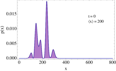
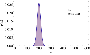
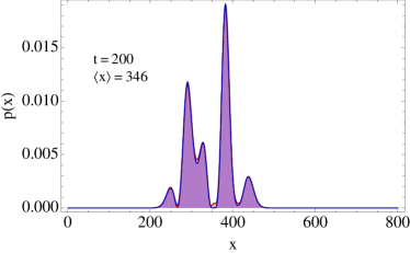
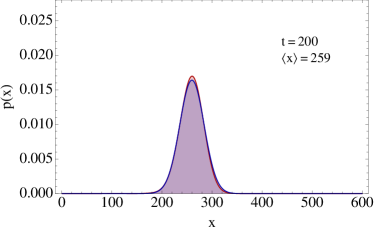
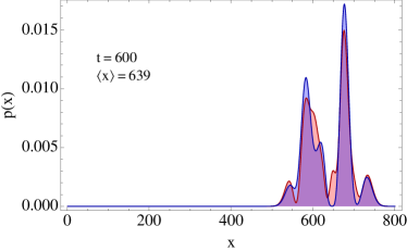
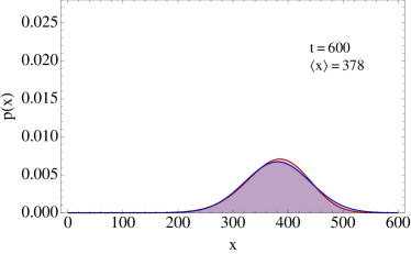
Figure 1: (Colors online) Test of the approximated evolution of Eq. (18) of the one dimensional Dirac automaton evolution. Left figure: here the state is a superposition of Hermite functions (the polynomials $H_{j}(x)$ multiplied by the Gaussian) peaked around $k_{0}=3\pi/10$. Right figure: here the initial state is Gaussian profile peaked around $k_{0}=0.1$. This figure is published in Ref. Bisio et al. (2015b).

IV Phenomenology

This section is devoted to the study of the various phenomenological effects of the QCA model presented in Section II. The aim of this analysis is to understand the properties of the QCA dynamics and compare its features to the known results about the dynamics of free quantum fields. The ultimate goal to identify experimental situation in which it is possible to falsify the validity of the QCA theory.

IV.1 Zitterbewegung

The first feature of the QCA dynamics we are going to explore (for a more complete presentation see Ref.Bisio et al. (2013)) is the appearence of a fluctuation of the position in the particle trajectory, the so called zitterbewegung.

The Zitterbewegung was first recognized by Schrödinger in 1930 Schrödinger (1930) who noticed that in the Dirac equation describing the free relativistic electron the velocity operator does not commute with the Dirac Hamiltonian: the evolution of the position operator,exhibits a very fast periodic oscillation around the mean position with frequency $2mc^{2}$ and amplitude equal to the Compton wavelength $\hbar/mc$ with $m$ the rest mass of the relativistic particle. Zitterbewegung oscillations cannot be directly observed by current experimental techniques for an electron since the amplitude is very small $\approx 10^{-12}$ m. However, it can be seen in a number of solid-state, atomic-physics, photonic-cristal and optical waveguide simulators Lurié and Cremer (1970); Cannata and Ferrari (1991); Ferrari and Russo (1990); Cannata et al. (1990); Zhang (2008).

Here we focus on the one-dimensional Dirac QCA whose epression, introduced in Section II, is easily obtained as special case of Eq. (9)

$$U=\int_{-\pi}^{\pi}dk|k\rangle\langle k|\otimes U_{k}\quad U_{k}=\begin{pmatrix}ne^{-ik}&im\\ im&ne^{ik}\end{pmatrix}$$ (19)

The “position” operator $X$ corresponding to the representation $|x\rangle$ (i.e. such that $X|s\rangle|x\rangle=x|s\rangle|x\rangle$, $x\in\mathbb{Z}$) is defined as follows

$$X=\sum_{x\in\mathbb{Z}}x(I\otimes|x\rangle\langle x|).$$ (20)

and it provides the average location of a wavepacket in terms of $\langle\psi|X|\psi\rangle$. If we write the single particle in terms of its positive frequency and negative frequency components, i.e. $|\psi\rangle=c_{+}|\psi\rangle_{+}+c_{-}|\psi\rangle_{-}$, yhe time evolution of the mean value of the position operator $\langle\psi|X(t)|\psi\rangle$ is given by

$$x_{\psi}(t):=\langle\psi|X(t)|\psi\rangle=x_{\psi}^{+}(t)+x_{\psi}^{-}(t)+x_{\psi}^{\rm{int}}(t)$$

$$x_{\psi}^{\pm}(t):=\langle\psi_{\pm}|X(0)+Vt|\psi_{\pm}\rangle$$

$$x_{\psi}^{\rm{int}}(t):=2\Re[\langle\psi_{+}|X(0)-{Z}_{{X}}(0)+{Z}_{{X}}(t)|\psi_{-}\rangle]$$ (21)

where $V$ is a time independent operator corresponding to the group velocity and $Z_{X}(t)$ is the operator that gives the oscillatory motion (see Ref. Bisio et al. (2013) for the details). We notice that the interference between positive and negative frequency is responsible of the oscillating term $x_{\psi}^{\rm{int}}(t)$ whose magnitude is bounded by $1/m$ which in the usual dimensional units corresponds to the Compton wavelength $\hbar/mc$. These results show that $x_{\psi}^{\rm{int}}(t)$ is the automaton analogue of the Zitterbewegung for a Dirac particle. for $t\to\infty$ the term $2\Re[\langle\psi_{+}|{Z}_{{X}}(t)|\psi_{-}\rangle]$, which is responsible of the oscillation, goes to $0$ as $1/\sqrt{t}$ and only the additional shift contribution given by $2\Re[\langle\psi_{+}|X(0)-{Z}_{{X}}(0)|\psi_{-}\rangle]$ survives. In Fig. 2 one can se the simulation of the evolution of states with particle and antiparticle components smoothly peaked around some $k_{0}$.

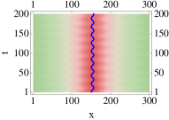
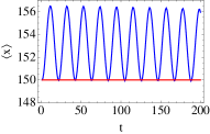
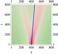
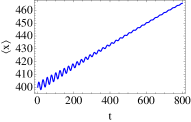
Figure 2: Zitterbewegung in the one dimensiona Dirac QCA. Top: The mass of the particle is $m=0.15$. The amplitudes of the superposition between positive and negative frequency states are $c_{+}=1/\sqrt{2}$ $c_{-}=i/\sqrt{2}$ respectively. The wavepacket is peaked around $k_{0}=0$. The shift and oscillation frequency are respectively $\langle\psi|X(0)+Z_{X}(0)|\psi\rangle=3.2$ and $\omega(0)/\pi=0.05$. Middle: $m=0.15$, $c_{+}=1/\sqrt{2}$, $c_{-}=1/\sqrt{2}$, $k_{0}=0$, $\sigma=40^{-1}$. The shift and oscillation frequency are $0$ and $0.13$, respectively. Bottom: $m=0.13$, $c_{+}=\sqrt{2/3}$, $c_{-}=1/\sqrt{3}$, $k_{0}=10^{-2}\pi$, $\sigma=40^{-1}$. In this case the particle and antiparticle contribution are not balanced and the average position drift velocity is thus $\langle\psi_{+}|V|\psi_{+}\rangle+\langle\psi_{-}|V|\psi_{-}\rangle=(|c_{+}|^{2}-|c_{-}|^{2})v(k_{0})=0.08$, corresponding to an average position $x_{\psi}^{+}(800)+x_{\psi}^{-}(800)=464$. Notice that for $t\to\infty$ the term $2\Re[\langle\psi_{+}|{Z}_{{X}}(t)|\psi_{-}\rangle$, which is responsible of the oscillation, goes to $0$. This figure is published in Ref. Bisio et al. (2013).

IV.2 Scattering against a potential barrier

In this section we study the dynamics of the one dimensional Dirac automaton in the presence of a potential. In the position representation the one particle evolution of the one dimensioanal Dirac QCA reads as follows:

$$U:=\sum_{x}\left(\begin{array}[]{ll}n|x-1\rangle\langle x|&-im|x\rangle\langle x|\\ -im|x\rangle\langle x|&n|x+1\rangle\langle x|\end{array}\right).$$ (24)

The presence of a potential $\phi(x)$, modifies the unitary evolution of Eq. (24) with a position dependent phase as follows (see also Ref Kurzyński (2008); Meyer (1997)):

$$U_{\phi}:=\sum_{x}e^{-i\phi(x)}\left(\begin{array}[]{ll}n|x-1\rangle\langle x|&-im|x\rangle\langle x|\\ -im|x\rangle\langle x|&n|x+1\rangle\langle x|\end{array}\right).$$

We now review the analysis (carried on in Ref. Bisio et al. (2013)) of the case in which $\phi(x):=\phi\,\theta(x)$ ($\theta(x)$ is the Heaviside step function) that is a potential step which is $0$ for $x<0$ and has a constant value $\phi\in[0,2\pi]$ for $x\geq 0$. Let us consider the situation in which, for $t\ll 0$, the state is a positive frequency wavepacket peaked around $\mathbf{k}_{0}$ that moves at group velocity $v(k_{0})$ and hits the barrier form the left. Then and one can show that for $t\gg 0$ the state is evolved into a superposition of a reflected and a transmitted wavepacket as follows (we use the notation of Eq. (16) adapted at the one-dimensional case):

$$\begin{split}|\psi(t)\rangle\xrightarrow{t\gg 0}\beta(k_{0})\int\!\!\frac{\mathop{\mathrm{d}k}}{\sqrt{2\pi}}\,g_{k_{0}}(k)e^{-i\omega(k)t}|u\rangle_{-k}|k\rangle+\\ {}+\tilde{\gamma}(k_{0})e^{-i\phi t}\int\!\!\frac{\mathop{\mathrm{d}k}}{\sqrt{2\pi}}\,\tilde{g}_{k^{\prime}_{0}}(k^{\prime})e^{-i\omega(k^{\prime})t}|u\rangle_{k^{\prime}}|k^{\prime}\rangle\end{split}$$

where we defined

$$k^{\prime}_{0}\mbox{ s.t. }\omega(k^{\prime}_{0})=\omega(k_{0})-\phi,$$

$$\tilde{\gamma}(k_{0}):={\gamma}(k_{0})\sqrt{\frac{v(k^{\prime}_{0})}{v(k_{0})}},\qquad\tilde{g}_{k^{\prime}_{0}}(k^{\prime})=\sqrt{\frac{v(k^{\prime}_{0})}{v(k_{0})}}{g}_{k^{\prime}_{0}}(k^{\prime})$$

(one can check $\int\!\!\frac{\mathop{\mathrm{d}k}}{\sqrt{2\pi}}\,|\tilde{g}_{k^{\prime}_{0}}(k^{\prime})|^{2}=1$), whose group velocities are $-v(k_{0})$ for the reflected wave packet and $v(k^{\prime}_{0})$ for the transmitted wave packet.

The probability of finding the particle in the reflected wavepacket is then $R=|\beta(k_{0})|^{2}$ (reflection coefficient) while the probability of finding the particle in the transmitted wavepacket is $T=|\tilde{\gamma}(k_{0})|^{2}$ (trasmission coefficient). The consistency of the result can be verified by checking that $R+T=1$. Clearly $\phi=0$ implies $R=0$ and increasing $\phi$ for a fixed $k$ increases the value of $R$ up to $R=1$. By further increasing $\phi$ a transmitted wave reappears and the reflection coefficient decreases. This is the so called “Klein paradox” which is originated by the presence of positive and negative frequency eigenvalues of the unitary evolution. The width of the $R=1$ region is an increasing function of the mass equal to $2\arccos(n)$ which is the gap between positive and negative frequency solutions.

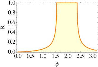
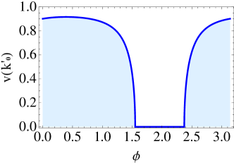
Figure 3: Reflection coefficient for $m=0.4$ and wave-vector of the incident particle $k_{0}=2$ as a function of the potential barrier height $\phi$. This Figure is published in Ref. Bisio et al. (2013).

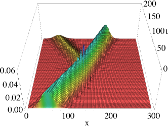
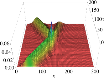
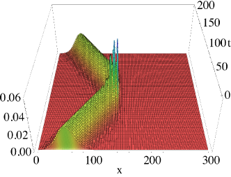
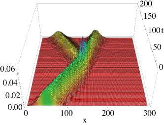
Figure 4: Simulations of the one dimensional Dirac automaton evolution with a square potential barrier. Here the automaton mass is $m=0.2$ while the barrier turns on at $x=140$. In the simulation the incident state is a smooth state of the form $|\psi(0)\rangle=\int\!\!\frac{\mathop{\mathrm{d}k}}{\sqrt{2\pi}}\,g_{k_{0}}(k)|+\rangle_{k}$ peaked around the positive frequency eigenstate $|+\rangle_{k_{0}}$ with $k_{0}=2$ and with $g_{k_{0}}$ a Gaussian having width $\sigma=15^{-1}$. The incident group velocity is $v(k_{0})=0.90$. The simulation is run for four increasing values of the potential $\phi$. Top-Left: Potential barrier height $\phi=1.42$, reflection coefficient $R=0.25$, velocity of the transmitted particle $v(k^{\prime}_{0})=0.63$. Top-Right: $\phi=1.55$, $R=0.75$, $v(k^{\prime}_{0})=0.1$. Bottom-Left: $\phi=2$, $R=0.1$, $v(k^{\prime}_{0})=0$. Bottom-Right: $\phi=2.4$, $R=0.50$, $v(k^{\prime}_{0})=0.33$. This Figure is published in Ref. Bisio et al. (2013).

In Fig. 3 we plot the reflection $R$ coefficient and the transmitted wave velocity group $v(k_{0}^{\prime})$ as a function of the potential barrier height $\phi$ with the incident wave packet having $k_{0}=2$ and $m=0.4$. From the figure it is clear that after a plateau with $R=1$ the reflection coefficient starts decreasing for higher potentials. In Fig. 4 we show the scattering simulation for four increasing values of the potential, say $\phi=1.42,\,1.55,\,2,\,2.4$.

IV.3 Travel-time and Ultra-high energy cosmic rays

The approximated evolution studied in Section III.1 provide a useful analytic tool for evaluating the macroscopic evolution of the automaton. We now consider an elementary experiment, based on particle fly-time, which compares the Dirac automaton evolution with the one given by the Dirac equation.

Consider a protonwith $m_{p}\approx 10^{-19}$ and wave-vector peaked around $k_{CR}\approx 10^{-8}$ in Planck units , with a spread $\sigma$ of the wave-vector. We ask what is the minimal time $t_{CR}$ for observing a complete spatial separation between the trajectory predicted by the cellular automaton model and the one described by the usual Dirac equation. Thus we require the separation between the two trajectories to be greater than $\hat{\sigma}=\sigma^{-1}$ the initial proton’s width in the position space. We approximate the state evolution of the wave-packet of the proton using the differential equation (18) for an initial Gaussian state. The time required to have a separation $\hat{\sigma}$ between the automaton and the Dirac particle is

$$t_{CR}\approx 6\frac{\hat{\sigma}}{m_{p}^{2}}.$$ (25)

and for $\hat{\sigma}=10^{2}\text{fm}$ (that is reasonable for a proton wave-packet) the flying time request for complete separation between the two trajectories is $t_{CR}\approx 6\times 10^{60}$ Planck times, i.e. $\approx 10^{17}s$, a value that is comparable with the age of the universe and then incompatible with a realistic setup.

IV.4 Phenomenology of the QCA Theory of Light

In this section we present an overview of the new phenomenology emerging from QCA theory of free electrodynamics presented in Section II. For a more detailed presentation we refer to Ref. Bisio et al. (2014).

IV.4.1 Frequency dependent speed of light

From Eq. (LABEL:eq:maxwell2) one has that the angular frequency of the electromagnetic waves is given by the modified dispersion relation

$$\omega(\mathbf{k})=2|\mathbf{n}_{\tfrac{\mathbf{k}}{2}}|.$$ (26)

and the usual relation $\omega(\mathbf{k})=|\mathbf{k}|$ is recovered in only the $|\mathbf{k}|\ll 1$ regime. The speed of light is the group velocity of the electromagnetic waves, i.e. the gradient of the dispersion relation. The major consequence of Eq. (26) is that the speed of light depends on the value of $\mathbf{k}$, as if the vacuum were a dispersive medium.

The phenomenon of a $\mathbf{k}$-dependent speed of light is also studied in the quantum gravity literature where many authors considered the hypothesis that the existence of an invariant length (the Planck scale) could manifest itself in terms of dispersion relations that differ from the usual relativistic one Ellis et al. (1992); Lukierski et al. (1995); ’t Hooft (1996); Amelino-Camelia (2001); Magueijo and Smolin (2002). In these models the $\mathbf{k}$-dependent speed of light $c(\mathbf{k})$, at the leading order in $k:=|\mathbf{k}|$, is expanded as $c(\mathbf{k})\approx 1\pm\xi k^{\alpha}$, where $\xi$ is a numerical factor of order $1$, while $\alpha$ is an integer. This is exactly what happens in our framework, where the intrinsic discreteness of the quantum cellular automata leads to the dispersion relation of Eq. (26) from which the following $\mathbf{k}$-dependent speed of light

$$c(\mathbf{k})\approx 1\pm 3\frac{k_{x}k_{y}k_{z}}{|\mathbf{k}|^{2}}\approx 1\pm\tfrac{1}{\sqrt{3}}k,$$ (27)

can be obtained by computing the modulus of the group velocity and power expanding in $\mathbf{k}$ with the assumption $k_{x}=k_{y}=k_{z}=\tfrac{1}{\sqrt{3}}k$, $k=|\mathbf{k}|$. The $\pm$ sign in Eq. (27) depends on whether we considered the $A^{+}(\mathbf{k})$ or the $A^{-}(\mathbf{k})$ Weyl QCA. This prediction can possibly be experimentally tested in the astrophysical domain, where tiny corrections are magnified by the huge time of flight. For example, observations of the arrival times of pulses originated at cosmological distances, like in some $\gamma$-ray burstsAmelino-Camelia et al. (1998); Abdo et al. (2009); Vasileiou et al. (2013); Amelino-Camelia and Smolin (2009), are now approaching a sufficient sensitivity to detect corrections to the relativistic dispersion relation of the same order as in Eq. (27).

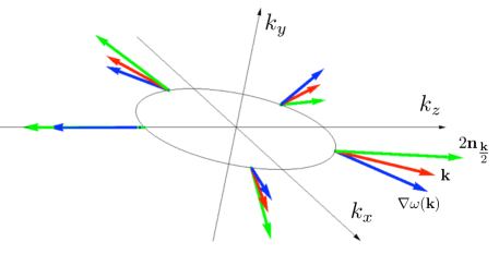
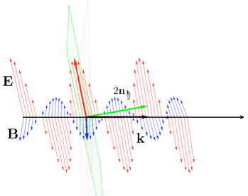
Figure 5: (colors online) Left: the graphics shows the vector $2\mathbf{n}_{\tfrac{\mathbf{k}}{2}}$ (in green), which is orthogonal to the polarization plane, the wavevector $\mathbf{k}$ (in red) and the group velocity $\nabla\omega(\mathbf{k})$ (in blue) as function of $\mathbf{k}$ for the value $|\mathbf{k}|=0.8$ and different directions. Right: A rectilinear polarized electromagnetic wave. We notice that the polarization plane (in green) is sligtly tilted with respect the plane orthogonal to $\mathbf{k}$ (in gray). This Figure is published in Ref. Bisio et al. (2014).

IV.4.2 Longitudinal polarization

A second distinguishing feature of Eq. (LABEL:eq:maxwell2) is that the polarization plane is neither orthogonal to the wavevector, nor to the group velocity, which means that the electromagnetic waves are no longer exactly transverse (see Fig. 5). The angle $\theta$ between the polarization plane and the plane orthogonal to $\mathbf{k}$ or $\nabla\omega(\mathbf{k})$ is of the order $\theta\approx 10^{-15}\mathrm{rad}$ for a $\gamma$-ray wavelength, a precision which is not reachable by the present technology. Since for a fixed $\mathbf{k}$ the polarization plane is constant, exploiting greater distances and longer times does not help in magnifying this deviation from the usual electromagnetic theory.

IV.4.3 Composite photons and modified commuation relations

Finally, the third phenomenological consequence of the QCA theory of light is the deviation from the exact Bosonic statistics due to the composite nature of the photon. As shown in Ref.Bisio et al. (2014), the choice of the function ${f}_{\mathbf{k}}(\mathbf{q})$ in Eq. (10) determines the regime where the composite photon can be approximately treated as a Boson. However, independently on the details of function ${f}_{\mathbf{k}}(\mathbf{q})$, one can prove that a Fermionic saturation of the Boson is not visible, e.g. for the most powerful laser Dunne (2007) one has a approximately an Avogadro number of photons in $10^{-15}$cm³, whereas in the same volume on has around $10^{90}$ Fermionic modes. Another test for the composite nature of photons is provided by the prediction of deviations from the Planck’s distribution in Blackbody radiation experiments. A similar analysis was carried out in Ref. Perkins (2002), where the author showed that the predicted deviation from Planck’s law is less than one part over $10^{-8}$, well beyond the sensitivity of present day experiments.

V Future perspectives

We conclude this paper with an overview of the future developments of the research program on QCA for Field Theory.

V.1 Lorentz covariance and Deformed Relativity

Because of the intrinsic discreteness of the model, a dynamical evolution described in terms of a QCA cannot satisfy the usual Lorentz covariance, which must break down at the Planck scale. Moreover the very notions of spacetime and boosted reference frame break down at small scales, and need a thoughtful reconsideration. In Ref. Bisio et al. (2015c) a definition of reference frame was introduced in a background-free scenario, in terms of labelling of irreducible representations of the group $G$. The Lorentz symmetry is then recovered by imposing a generalized relativity principle on possible changes of reference frame, allowing only those changes that leave the automaton invariant. A preliminary analysis of the one-dimensional case can be found in Ref. Bibeau-Delisle et al. (2013), where only the necessary condition of preserving the dispersion relation was considered. Focusing on the one dimensional Dirac QCA we have

$$\omega(k)=\arccos(\sqrt{1-m^{2}}\cos(k))$$ (28)

and one can see that in the $k\ll 1$,$m\ll 1$ limit Eq. (28) reduces to the usual relativistic dispersion relation $\omega^{2}=k^{2}+m^{2}$. It is also immediate to check that the automaton dispersion relation of Eq. (28) is not invariant under standard Lorentz transformation. In order to preserve Eq. (28) one needs to introduce a non-linear representation of the Lorentz transformation in the wave-vector space—as proposed in the so called deformed special relativity (DSR) models Amelino-Camelia (2002a); Amelino-Camelia and Piran (2001); Amelino-Camelia (2002b, 2001); Magueijo and Smolin (2002, 2003).

In Ref. Bisio et al. (2015c) the boosts preserving the three-dimensional Weyl automaton were then derived in the form of the following non-linear representation of the Lorentz group

$${L}^{D}_{\beta}:=\mathcal{D}^{-1}\circ L_{\beta}\circ\mathcal{D},$$ (29)

where $\mathcal{D}:{\mathbb{R}}^{4}\to{\mathbb{R}}^{4}$ is a non-linear map. The specific form of $\mathcal{D}$ gives rise to a particular frequency/wave-vector Lorentz deformation.

These ideas can also be applied to the three-dimensional Dirac QCA. In this case one can show that a change of the rest mass should be involved in the representation of boosts, in order to obey our generalized relativity principle. Interestingly, this unexpected feature gives rise to an emergent space-time with a non-linear de Sitter symmetry instead of the Lorentz one.

Another challenging line of research is to characterize the emergent spacetime of the QCA framework. The DSR models provide a complete description of Lorentz symmetry in frequency/wave-vector space but there are heuristic ways to extend this framework to the position-time space. Relative locality Amelino-Camelia et al. (2011, 2013), non-commutative spacetime Connes and Lott (1991) and Hopf algebra symmetries Lukierski et al. (1991); Majid and Ruegg (1994) have been considered in order to give a real space formulation of deformed relativity.

Finally, we would like to stress that space-time emerges from: i) the structure of the group $G$, ii) the specific expression of the automaton and iii) the generalized relativity principle, while all these concepts do not require any space-time background. Thus, outside the limits in which the relativistic approximations hold, the very structure of our usual space-time break down, substituted by other counterintuitive effects. In particular this is true in all physical situations where the discrete structure of the lattice $G$ becomes relevant.

V.2 Thermodynamics of free ultra-relativistic particles and QCA

Most of the analysis that we presented in this paper was focused on the dynamics of one particle state and the deviations of this kinematics from the usual relativistic one. On the other hand, it would be interesting to explore the QCA phenomenology when the number of particle goes to infinity, namely a thermodynamic limit. Since the QCA we are considering descrive a non-interacting dynamics, the thermodynamic that will emerge will describe a gas of free particles. However, since the dispersion relation of the QCA differs from the relativistic one, the density of states will be different.

In the case of free fermions this will result in a shift of the Fermi energy that could become relevant when the number of fermions becomes very large. One could for example analyze how the Chandrasekhar limit of white dwarfs is modified in this context (see Ref. Amelino-Camelia et al. (2012); Camacho (2006) for a similar analysis in a different context).

V.3 Interacting extensions

The theory of linear QCAs naturally leads to free quantum field theories. In order to introduce interactions, one needs to relax the linearity assumption. This can be done by splitting the computational step in two stages, the first one acting linearly, and the second one representing a nonlinear and completely local evolution. This can be motivated in terms of a time-local gauge symmetry that must preserve some local degree of freedom, in particular the local number of excitations. This simple modification of the linear automaton introduces a non-trivial interaction, making the automaton non-trivially reducible to a quantum walk. Preliminary analysis shows that this minimal relaxation of linearity is sufficient to give rise to couplings that might reproduce the phenomenology of quantum electrodynamics.

References

- Bisio et al. (2015a) A. Bisio, G. M. D’Ariano, P. Perinotti, and A. Tosini, Foundations of Physics 45, 1137 (2015a).
- von Neumann (1966) J. von Neumann, Theory of self-reproducing automata (University of Illinois Press, Urbana and London, 1966).
- Hooft (2014) G. Hooft, arXiv preprint arXiv:1405.1548 (2014).
- Elze (2014) H.-T. Elze, Physical Review A 89, 012111 (2014).
- Feynman (1982) R. Feynman, International journal of theoretical physics 21, 467 (1982).
- Schumacher and Werner (2004) B. Schumacher and R. Werner, Arxiv preprint quant-ph/0405174 (2004).
- Arrighi et al. (2011) P. Arrighi, V. Nesme, and R. Werner, Journal of Computer and System Sciences 77, 372 (2011).
- Gross et al. (2012) D. Gross, V. Nesme, H. Vogts, and R. Werner, Communications in Mathematical Physics , 1 (2012).
- Grossing and Zeilinger (1988) G. Grossing and A. Zeilinger, Complex Systems 2, 197 (1988).
- Aharonov et al. (1993) Y. Aharonov, L. Davidovich, and N. Zagury, Physical Review A 48, 1687 (1993).
- Ambainis et al. (2001) A. Ambainis, E. Bach, A. Nayak, A. Vishwanath, and J. Watrous, in Proceedings of the thirty-third annual ACM symposium on Theory of computing (ACM, 2001) pp. 37–49.
- Reitzner et al. (2011) D. Reitzner, D. Nagaj, and V. Buek, Acta Physica Slovaca. Reviews and Tutorials 61, 603 (2011).
- Childs et al. (2003) A. M. Childs, R. Cleve, E. Deotto, E. Farhi, S. Gutmann, and D. A. Spielman, in Proceedings of the thirty-fifth annual ACM symposium on Theory of computing (ACM, 2003) pp. 59–68.
- Ambainis (2007) A. Ambainis, SIAM Journal on Computing 37, 210 (2007).
- Magniez et al. (2007) F. Magniez, M. Santha, and M. Szegedy, SIAM Journal on Computing 37, 413 (2007).
- Farhi et al. (2007) E. Farhi, J. Goldstone, and S. Gutmann, arXiv preprint quant-ph/0702144 (2007).
- D’Ariano (2010) G. D’Ariano, CP1232 Quantum Theory: Reconsideration of Foundations 5 (arXiv:1001.1088) 3 (2010).
- D’Ariano (2011) G. M. D’Ariano, Phys. Lett. A 376 (2011).
- Bisio et al. (2015b) A. Bisio, G. M. D’Ariano, and A. Tosini, Annals of Physics 354, 244 (2015b).
- D’Ariano and Perinotti (2014) G. M. D’Ariano and P. Perinotti, Phys. Rev. A 90, 062106 (2014).
- Bisio et al. (2014) A. Bisio, G. M. D’Ariano, and P. Perinotti, arXiv preprint arXiv:1407.6928 (2014).
- Arrighi et al. (2014) P. Arrighi, V. Nesme, and M. Forets, Journal of Physics A: Mathematical and Theoretical 47, 465302 (2014).
- Arrighi and Facchini (2013) P. Arrighi and S. Facchini, EPL (Europhysics Letters) 104, 60004 (2013).
- Farrelly and Short (2014) T. C. Farrelly and A. J. Short, Physical Review A 89, 012302 (2014).
- Farrelly and Short (2013) T. C. Farrelly and A. J. Short, arXiv preprint arXiv:1312.2852 (2013).
- D’Ariano et al. (2014a) G. M. D’Ariano, N. Mosco, P. Perinotti, and A. Tosini, Physics Letters A 378, 3165 (2014a).
- D’Ariano et al. (2014b) G. D’Ariano, N. Mosco, P. Perinotti, and A. Tosini, arXiv preprint arXiv:1410.6032 (2014b).
- Ellis et al. (1992) J. Ellis, N. Mavromatos, and D. V. Nanopoulos, Physics Letters B 293, 37 (1992).
- Lukierski et al. (1995) J. Lukierski, H. Ruegg, and W. J. Zakrzewski, Annals of Physics 243, 90 (1995).
- ’t Hooft (1996) G. ’t Hooft, Class. Quantum Grav. 13, 1023 (1996).
- Amelino-Camelia (2001) G. Amelino-Camelia, Physics Letters B 510, 255 (2001).
- Magueijo and Smolin (2002) J. Magueijo and L. Smolin, Phys. Rev. Lett. 88, 190403 (2002).
- De Broglie (1934) L. De Broglie, Une nouvelle conception de la lumière, Vol. 181 (Hermamm & Cie, 1934).
- Jordan (1935) P. Jordan, Zeitschrift für Physik 93, 464 (1935).
- Kronig (1936) R. d. L. Kronig, Physica 3, 1120 (1936).
- Perkins (1972) W. Perkins, Physical Review D 5, 1375 (1972).
- Perkins (2002) W. Perkins, International Journal of Theoretical Physics 41, 823 (2002).
- Bisio et al. (2013) A. Bisio, G. M. D’Ariano, and A. Tosini, Phys. Rev. A 88, 032301 (2013).
- Succi and Benzi (1993) S. Succi and R. Benzi, Physica D: Nonlinear Phenomena 69, 327 (1993).
- Bialynicki-Birula (1994) I. Bialynicki-Birula, Physical Review D 49, 6920 (1994).
- Meyer (1996) D. Meyer, Journal of Statistical Physics 85, 551 (1996).
- Schrödinger (1930) E. Schrödinger, Über die kräftefreie Bewegung in der relativistischen Quantenmechanik (Akademie der wissenschaften in kommission bei W. de Gruyter u. Company, 1930).
- Lurié and Cremer (1970) D. Lurié and S. Cremer, Physica 50, 224 (1970).
- Cannata and Ferrari (1991) F. Cannata and L. Ferrari, Physical Review B 44, 8599 (1991).
- Ferrari and Russo (1990) L. Ferrari and G. Russo, Physical Review B 42, 7454 (1990).
- Cannata et al. (1990) F. Cannata, L. Ferrari, and G. Russo, Solid State Communications 74, 309 (1990).
- Zhang (2008) X. Zhang, Phys. Rev. Lett. 100, 113903 (2008).
- Kurzyński (2008) P. Kurzyński, Physics Letters A 372, 6125 (2008).
- Meyer (1997) D. A. Meyer, International Journal of Modern Physics C 8, 717 (1997).
- Amelino-Camelia et al. (1998) G. Amelino-Camelia, J. Ellis, N. Mavromatos, D. V. Nanopoulos, and S. Sarkar, Nature 393, 763 (1998).
- Abdo et al. (2009) A. Abdo, M. Ackermann, M. Ajello, K. Asano, W. Atwood, M. Axelsson, L. Baldini, J. Ballet, G. Barbiellini, M. Baring, et al., Nature 462, 331 (2009).
- Vasileiou et al. (2013) V. Vasileiou, A. Jacholkowska, F. Piron, J. Bolmont, C. Couturier, J. Granot, F. Stecker, J. Cohen-Tanugi, and F. Longo, Physical Review D 87, 122001 (2013).
- Amelino-Camelia and Smolin (2009) G. Amelino-Camelia and L. Smolin, Physical Review D 80, 084017 (2009).
- Dunne (2007) M. Dunne, in Conference on Lasers and Electro-Optics/Pacific Rim (Optical Society of America, 2007) pp. 1–2.
- Bisio et al. (2015c) A. Bisio, G. M. D’Ariano, and P. Perinotti, arXiv preprint arXiv:1503.01017 (2015c).
- Bibeau-Delisle et al. (2013) A. Bibeau-Delisle, A. Bisio, G. M. D’Ariano, P. Perinotti, and A. Tosini, arXiv preprint arXiv:1310.6760 (2013).
- Amelino-Camelia (2002a) G. Amelino-Camelia, International Journal of Modern Physics D 11, 35 (2002a).
- Amelino-Camelia and Piran (2001) G. Amelino-Camelia and T. Piran, Physical Review D 64, 036005 (2001).
- Amelino-Camelia (2002b) G. Amelino-Camelia, Modern Physics Letters A 17, 899 (2002b).
- Magueijo and Smolin (2003) J. Magueijo and L. Smolin, Physical Review D 67, 044017 (2003).
- Amelino-Camelia et al. (2011) G. Amelino-Camelia, L. Freidel, J. Kowalski-Glikman, and L. Smolin, International Journal of Modern Physics D 20, 2867 (2011).
- Amelino-Camelia et al. (2013) G. Amelino-Camelia, V. Astuti, and G. Rosati, The European Physical Journal C 73, 1 (2013).
- Connes and Lott (1991) A. Connes and J. Lott, Nuclear Physics B-Proceedings Supplements 18, 29 (1991).
- Lukierski et al. (1991) J. Lukierski, H. Ruegg, A. Nowicki, and V. N. Tolstoy, Physics Letters B 264, 331 (1991).
- Majid and Ruegg (1994) S. Majid and H. Ruegg, Physics Letters B 334, 348 (1994).
- Amelino-Camelia et al. (2012) G. Amelino-Camelia, N. Loret, G. Mandanici, and F. Mercati, International Journal of Modern Physics D 21 (2012).
- Camacho (2006) A. Camacho, Classical and Quantum Gravity 23, 7355 (2006).
- Albeverio et al. (2009) S. Albeverio, R. Cianci, and A. Y. Khrennikov, P-Adic Numbers, Ultrametric Analysis, and Applications 1, 91 (2009).
- Takeda et al. (1998) M. Takeda, N. Hayashida, K. Honda, N. Inoue, K. Kadota, F. Kakimoto, K. Kamata, S. Kawaguchi, Y. Kawasaki, N. Kawasumi, et al., Physical Review Letters 81, 1163 (1998).