Morphology and kinematics of the gas envelope of the variable AGB star $\pi^{1}$ Gruis

Abstract

Observations of the ¹²CO(3-2) emission of the circumstellar envelope (CSE) of the variable star $\pi^{1}$ Gru using the compact array (ACA) of the ALMA observatory have been recently made accessible to the public. An analysis of the morphology and kinematics of the CSE is presented with a result very similar to that obtained earlier for ¹²CO(2-1) emission by Chiu et al. (2006) using the Sub-Millimeter Array. A quantitative comparison is made using their flared disk model. A new model is presented that provides a significantly better description of the data, using radial winds and smooth evolutions of the radio emission and wind velocity from the stellar equator to the poles.

1 Introduction

$\pi^{1}$ Gruis (HIP 110478) is an SRb variable star of spectral type S5,7, namely in the transition between being oxygen and carbon dominated ([Piccirillo 1980], [Scalo & Ross 1976], [Van Eck et al. 2011]), with a pulsation period of 195 days ([Pojmanski & Maciejewski 2005]), a mean luminosity of $\sim 7240$ solar luminosities, an effective temperature of $\sim 3100$ K ([Van Eck et al. 1998]) and technetium lines in its spectrum (Jorissen et al. 1993). According to Mayer et al. (2014), its original mass was around two solar masses but has now dropped to 1.5 only. It is close to the Sun, only 163 pc ([van Leeuwen et al. 2007]) and very bright, making it one the best known S stars.

It has a companion at a projected angular distance of $2.8^{\prime\prime}$, meaning $\sim 460$ AU, a position angle of $200^{\circ}$ ([Proust et al. 1981]) with an apparent visual magnitude of 6.55 ([Ducati 2002], [Ake & Johnson 1992]) and an orbital period of over 6200 years ([Mayer et al. 2014]). Its large scale environment has been recently observed by Mayer et al. (2014) at 70 $\mu$m and 160 $\mu$m using Herschel/PACS images and interferometric observations from the VLTI/AMBER archive. They observe an arc east of the star at a projection distance of $\sim 38^{\prime\prime}$, suggesting interaction with the companion.

Single dish observations of the CSE have been made by Knapp et al. (1999) using the 10-meter telescope of the Caltech Submillimeter Observatory in CO(2-1) and by Winters et al. (2003) at ESO with the SEST 15-m antenna in both CO(1-0) and CO(2-1). The line profiles display extended wings with a double horned structure at low velocity. The mass-loss rate is measured to be $\sim 2.7\times 10^{-6}$ M_⊙ yr^-1, with an expansion velocity of 14.5 kms^-1 ([Guandalini & Busso 2008]) and a dust to gas ratio of 380 ([Groenewegen & de Jong 1998]); Sahai (1992) was first to map the CSE using the 15 meter Swedish-ESO Sub-millimeter telescope, scanning over the star in steps of half a beam, and to give direct evidence for a fast bipolar outflow.

High spatial resolution observations of the CO(2-1) emission were recently made by Chiu et al. (2006), here referred to as C2006, using the Sub-Millimeter Array, producing channel maps and position-velocity diagrams interpreted as resulting from a slowly expanding equatorial disk and a fast bipolar outflow. They show that the expansion at low velocities ($<$15 kms^-1 ) is elongated east-west and at high velocities ($>$25 kms^-1 ) is displaced north (red-shifted) and south (blue-shifted). They propose a model describing the low velocity component as a flared disk with a central cavity of radius 200 AU and an expansion velocity of 11 kms^-1 , inclined by $55^{\circ}$ with respect to the line of sight; and the high velocity component as a bipolar outflow that emerges perpendicular to the disk with a velocity of up to $\sim 45$ kms^-1.

Recently, ALMA observations of the CO(3-2) emission of the circumstellar envelope, using the ALMA compact array ACA, have been made publicly available (ALMA01004143). With a spatial resolution comparable with that obtained in the lower velocity range by C2006, they usefully complement their CO(2-1) observations. The present work presents an analysis and modeling of these new data.

2 Observations, data reduction and data selection

The star was observed on October 8${}^{\text{th}}$, 2013, for six minutes on the line using the compact array (ACA, seven 7-m antennae) configuration with beam size and position angle of $4.45^{\prime\prime}\times 2.48^{\prime\prime}$ and $-84^{\circ}$. The data have been reduced by the ALMA staff. The line Doppler velocity spectra are available in sixty bins of 2 kms^-1 between $-60$ kms^-1 and 60 kms^-1 after subtraction of a local standard of rest Doppler velocity of $-11$ kms^-1 ; the measured value given by Mayer et al. (2014) is $-11.7\pm 2.5$ kms^-1 but we round it up to have the origin between bins 30 and 31. Figure 1 (left) displays the line profile, with a double-horn structure at low velocities and wings extending to $-36$ kms^-1 and 40 kms^-1 and a mean value of $-0.4$ kms^-1. In what follows we restrict the analysis to this velocity interval. Both horns are of similar intensities in the present data while the blue-shifted horn dominates in the C2006 data and the red-shifted horn in the data of Knapp et al. (1999). Figure 1 (right) displays the distribution of the number of pixels and velocity bins over the measured flux density. The peak associated with the effective noise has an rms value of 6.2 mJy arcsec^-2.

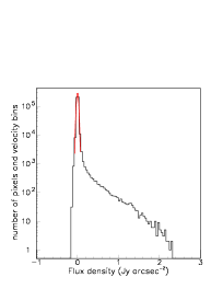
Figure 1: Left: Integrated flux densities (Jy) as a function of Doppler velocities (kms^-1). Right: Distribution of the number of pixels and velocity bins as a function of measured flux density in Jy arcsec^-2. The line is a Gaussian fit centred at the origin with an rms value 6.2 mJy arcsec^-2.

Figure 2 displays the $y$ and $z$ distributions ($y$ points east and $z$ points north) centred on the peak of maximal emission taken as origin of coordinates: pixels are $0.5^{\prime\prime}\times 0.5^{\prime\prime}$ and the mean values after centering are $0.28^{\prime\prime}$ and $0.07^{\prime\prime}$ respectively, smaller than the pixel size. Also shown is the sky map of the flux integrated over Doppler velocity and multiplied by $R=\sqrt{y^{2}+z^{2}}$ in Jy arcsec^-1 kms^-1 in order to better reveal inhomogeneities at large distances (a $r^{-2}$ dependence of the flux density means a $R^{-1}$ dependence of the integrated flux). In what follows, we limit the analysis to $R<7^{\prime\prime}$ in order to keep the effects of noise and side lobes at a low level and apply a 3$\sigma$ cut to the measured flux densities (0.02 Jy arcsec^-2). From Mamon et al. (1988) we estimate the effective radius of dissociation of CO molecules by the interstellar UV radiation to be $\sim 6700$ AU, namely $\sim 41^{\prime\prime}$.

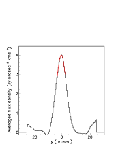
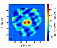
Figure 2: Angular projected distances $y$ (left) and $z$ (middle) distributions for pixels where data are available and for the Doppler velocity in the [$-36$ kms^-1 , 40 kms^-1] interval. The curves are Gaussian fits having mean values of $0.28^{\prime\prime}$ and $0.07^{\prime\prime}$ respectively. Their sigma values are 3.38^′′ and 1.98^′′ respectively. Right: sky map of the flux integrated over Doppler velocity and multiplied by $R=\sqrt{y^{2}+z^{2}}$ in Jy kms^-1 arcsec^-1 (this trivially produces a dip at the origin). The beam is shown in the lower left corner.

3 Morphology and kinematics of the observed CSE

Figure 3 displays channel maps and Figure 4 (left) maps the mean Doppler velocity over the plane of the sky. The data are qualitatively similar to those published by C2006 for CO(2-1).

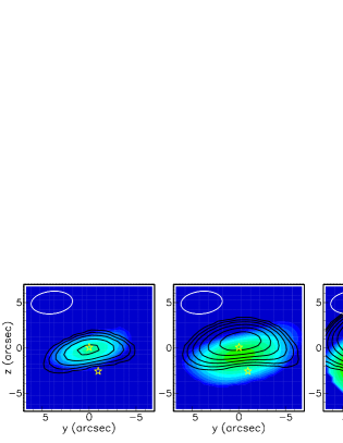
Figure 3: Sky maps ($y$ and $z$ in arcseconds) of the integrated flux (Jy kms^-1 arcsec^-2) in Doppler velocity intervals of, in absolute value and from left to right, 27 to 36 kms^-1, 18 to 27 kms^-1, 9 to 18 kms^-1 and 0 to 9 kms^-1. Colored maps are for negative velocities and contours for positive velocities in a same interval of $|V_{x}|$. A same logarithmic scale is used for all panels. Stars indicate the position of the primary and its companion. The beam is shown in the upper left corner of each panel.

They give evidence for a north-south wind perpendicular to the east-west elongation of the emission seen on the channel maps, as very clearly evidenced from their dependences on position angle $\varphi=\tan^{-1}(z/y)+\pi$, measured clockwise from west (Figure 4, middle and right), well described by simple sine wave fits of the form $35.6+13.0\sin(2\varphi+101^{\circ})$ (in Jy kms^-1 arcsec^-1) and $-0.49-6.92\sin(\varphi+7^{\circ})$ (in kms^-1). The mean Doppler velocity displayed in the right panel of the figure is defined as $\sum{V_{x}f(R,\varphi,V_{x})}/\sum{f(R,\varphi,V_{x})}$ where the sums run over Doppler velocities and over pixels contained in a wedge corresponding to a given $\varphi$ bin.

The contribution of the present observations to our understanding of the physical properties of the CSE of $\pi^{1}$ Gru is not sufficient to justify a detailed analysis of the kind presented by C2006, which would essentially repeat what they have already done. We limit instead our discussion of the present data to the modelling of the morphology and kinematics of the CSE using the concept of effective density, which we define as $\rho(x,y,z)=f(y,z,V_{x})\text{d}V_{x}/\text{d}x$. Here, $x$ is measured along the line of sight away from the observer (positive $x$ values are red-shifted) and $f(y,z,V_{x})$ is the measured flux density in pixel $(y,z)$ at Doppler velocity $V_{x}$. With this definition, the integrated flux measured in pixel $(y,z)$ is $F(y,z)=\int f(y,z,V_{x})\text{d}V_{x}=\int\rho(x,y,z)\text{d}x$. The effective density is proportional to the gas density but depends also on the temperature, the population of the emitting state and the emission and absorption probabilities.

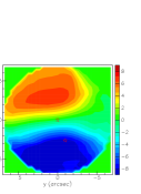
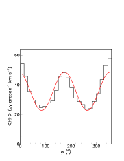
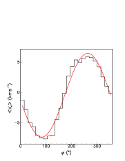
Figure 4: Left: sky map of the mean Doppler velocity (in kms^-1). Stars indicate the position of the primary and its companion. Middle: dependence on $\varphi$ of the flux integrated over Doppler velocity, averaged over $R$ and multiplied by $R=\sqrt{(y^{2}+z^{2}}$ in Jy arcsec^-1 kms^-1. Right: dependence on $\varphi$ of the mean Doppler velocity (kms^-1) averaged over $R$. The curves are sine wave fits of the form $35.6+13.0\sin(2\varphi+101^{\circ})$ (middle) and $-0.49-6.92\sin(\varphi+7^{\circ})$ (right).

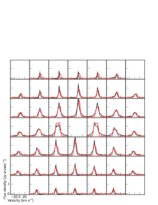
Figure 5: Spectral map of the present ACA data restricted to the region $R<7^{\prime\prime}$. Each pixel is $2^{\prime\prime}\times 2^{\prime\prime}$. The red curves are the best fit using the C2006 model. The central pixel is excluded from the fit.

In the present data, the very high velocity winds, up to 80 kms^-1, hinted at by Knapp et al. (1999) and C2006 would require longer observation times to be solidly established. Yet, the winds observed here extend over some $\pm 40$ kms^-1, which is quite a large span, and join smoothly to the low velocity profile. As the high spatial resolution C2006 data cover only $\pm 25$ kms^-1, the contribution of the present data is significant in this respect.

4 Flared disk model of the CSE

In a first step, we reproduce the results obtained by C2006 for CO(2-1). Namely the emission is confined to a flared disk having inner radius $r_{min}$, inner thickness $2z_{min}$ and a wedge angle $\pm\beta_{wedge}$. The orientation of its axis is defined by two angles, $\theta$ measuring its inclination with respect to the line of sight and $\psi$ measuring the position angle of its projection on the sky plane counter clockwise from north. We take the effective density proportional to $r^{-n}$ and the wind velocity radial with constant intensity $v_{rad}$ . We use a pixel size of $2^{\prime\prime}\times 2^{\prime\prime}$ without convolving the model by the beam and integrate along the line of sight up to $r=41^{\prime\prime}$, the mean UV dissociation radius. A Gaussian smearing of $\pm 2$ kms^-1 is included as in C2006. The values of the parameters giving the best fit are compared in Table 1 with the values found by Chiu et al. for CO(2-1). They are very close to each other. Note that the $r^{0.25}$ dependence of the flux of matter found by C2006 and the $r^{-0.7}$ dependence of the temperature that they use cannot be directly compared with the $r^{-2.03}$ dependence of the effective density used in our model, but both give adequate descriptions of the observations. The measured spectral map is compared with the model result in Figure 5. As found earlier by C2006 for CO(2-1), the model is seen to give a good qualitative description of the data but important deviations are observed. In particular the high wind velocity wings are obviously not reproduced by the model: the value of $v_{rad}$ is determined by the double-horned profile at low velocities and cannot produce Doppler velocities in excess of $v_{rad}$.

Table 1: Results of the C2006 model fits for CO(2-1) and CO(3-2).

Parameter	C2006 CO(2-1)	This work CO(3-2)
$\theta$	$145^{\circ}$	$140^{\circ}$
$\psi$	$6^{\circ}$	$6^{\circ}$
$V_{rad}$	11 kms-1	12.5 kms-1
$z_{min}$	$0.84^{\prime\prime}$	$1.0^{\prime\prime}$
$r_{min}$	$1.31^{\prime\prime}$	$1.3^{\prime\prime}$
$\beta_{wedge}$	$25^{\circ}$	$25^{\circ}$
$n$	-	2.03

5 A new model of the CSE

In order to improve on the C2006 model, one needs therefore to account for the presence of higher wind velocities than obtained from this model. Figure 6 displays position- velocity diagrams in the $V_{x}$ vs $\varphi$ plane for two different intervals of $R$ (the term is normally used in Cartesian coordinates but the information carried by such diagrams is of the same nature in polar coordinates). It shows continuity between low and high absolute values of the Doppler velocity and between low and high values of $R$. This suggests a smooth variation of the expansion velocity from the star equator, where the disk stands, to the star poles on the star axis perpendicular to the disk rather than a bipolar jet confined around the star axis. This had been already remarked by C2006 who proposed an explanation in terms of “material punched out of the disk by the bipolar outflow” and/or a “bipolar outflow simply having a very large opening angle”.

We construct therefore a new model allowing for continuity from equator to poles. A first exploration of different parameterizations suggested allowing for the effective density to extend to small values of $r$, and using a much smaller smearing of the Doppler velocities than assumed in C2006. In addition, it showed that adding rotation about the star axis does not bring significant improvement. On this basis, we write the radial expansion velocity as $V_{pole}\exp(-0.5\cos^{2}\alpha/\sigma_{pole}^{2})$ where $\alpha$ is the stellar latitude and the effective density as $\rho=\rho_{0}r^{-n}(\cos\alpha)^{p}[1-\exp(-0.5r^{2}/\sigma_{cut}^{2})]$ namely five parameters to be adjusted. In addition we include four additional parameters: the direction of the star axis, measured by $\theta$ and $\psi$ as before, the smearing parameter $\sigma_{v}$ and a small shift $\delta v$ of the origin of the Doppler velocity scale. The best fit value of $\chi^{2}$ is divided by 2.9 with respect to the C2006 model fit and the corresponding values of the model parameters are listed in Table 2. The value of $\rho_{0}$, obtained from the normalization between data and model, is 144 Jy arcsec^-3kms^-1. The fit to the spectral map is illustrated in Figure 7.

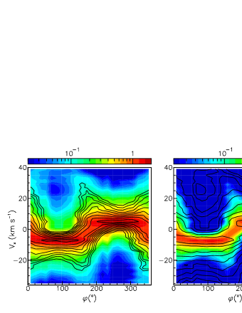
Figure 6: Position-velocity diagrams in the Doppler velocity $V_{x}$ vs position angle $\varphi=\tan^{-1}(z/y)+\pi$ for $R<3^{\prime\prime}$ (left) and $3^{\prime\prime}<R<7^{\prime\prime}$ (right). Contours in the left (right) panel correspond to the right (left) panel. The colour scale is in the unit of Jy arcsec^-2.

Table 2: Best fit values of the parameters in the new model. The quoted “uncertainties” list the amounts by which a parameter has to be changed for $\chi^{2}$ to increase by 5%.

Parameter	$\theta$ (∘)	$\psi$ (∘)	$V_{pole}$ (kms-1)	$\sigma_{pole}$ (kms-1)	$n$	$p$	$\sigma_{cut}$ (arcsec)	$\sigma_{v}$ (kms-1)	$\delta v$ (kms-1)
Best fit value	140	6	64	0.55	3.51	4.1	3.3	0.2	-1.2
“Uncertainty”	2	5	3	0.08	0.12	0.8	0.4	$<1.2$	0.3

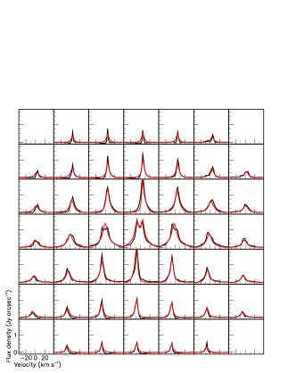
Figure 7: Spectral map of the present ACA data restricted to the region $0.75^{\prime\prime}<R<7^{\prime\prime}$. Each pixel is $2^{\prime\prime}\times 2^{\prime\prime}$. The red curves are the best fit using the new model (Table 2).

The dependence on stellar latitude of the radial expansion velocity and of the effective density is illustrated in Figure 8. The relative crudeness of the present model does not allow for a reliable quantitative evaluation of the uncertainties attached to the model parameters. However, we can measure the sensitivity of the quality of the best fit, i.e. the value of $\chi^{2}$, to the values taken by the model parameters as proportional to the quantity by which they must be changed to increase the value of $\chi^{2}$ by $\sim 5\%$. These values are listed in Table 2. They ignore correlations between parameters, such as between $\rho_{0}$ and $\rho$. We checked that accounting for a velocity gradient does not significantly improve the quality of the best fit. While the new model succeeds to account for the observed high velocity wings, it underestimates the importance of the double horn structure (Figure 9). Figure 10 displays sky maps of individual velocity bins in the horn region in an attempt to improve the quality of the best fit. It shows that the horns populate low $y$ regions at opposite $z$ values while the velocities in between the horns populate a low $z$ region with a broader $y$ extension. We failed to find a simple modification of the new model that would account for this feature.

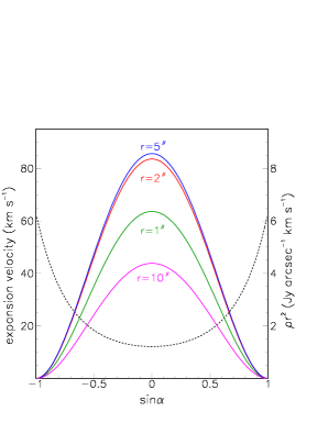
Figure 8: Dependence on stellar latitude of the radial expansion velocity $V_{rad}$ and effective density $\rho$ multiplied by $r^{2}$ corresponding to the best fit (Table 2). The effective density curves are for $r=1^{\prime\prime}$, $2^{\prime\prime}$, $5^{\prime\prime}$ and $10^{\prime\prime}$ as labelled and their values can be read from the right-hand scale.

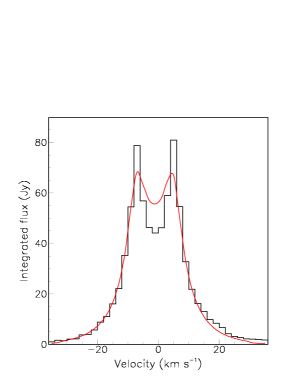
Figure 9: Doppler velocity spectrum of the present ACA data restricted to the region $R<7^{\prime\prime}$ and excluding the central $2^{\prime\prime}\times 2^{\prime\prime}$ pixel. The red curve is the best fit using the new model.

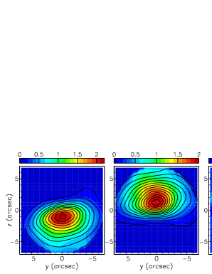
Figure 10: Sky maps of the double-horned structure for selected Doppler velocity bins. Extreme left: Doppler velocity bin of the blue-shifted horn. Contours show the map of the bins immediately below and above the horn bin. Central left: Doppler velocity bin of the red-shifted horn. Contours show the map of the bins immediately below and above the horn bin. Central right: horn velocity bins with the average of the neighbour bins subtracted. The upper population corresponds to the red-shifted horn, the lower population to the blue-shifted horn. Extreme right: the average of the three central Doppler velocity bins between the horns. The colour scales are in the unit of Jy arcsec^-2.

6 Discussion and conclusion

The new model brings a significant improvement over the flared disk model of C2006 and shows that there is no need for assuming the expansion to be confined to a flared disk having sharp boundaries. A similar model has been used to describe AGB stars, such as RS Cnc and EP Aqr, having a lower mass loss rate, at the scale of $10^{-7}$ rather than $10^{-6}$ M_⊙ yr^-1  ([Hoai et al. 2014], [Nhung et al. 2015a], [Nhung et al. 2015b]). However, in the present case, the effective density displays a strong oblateness while for the lower mass stars it is nearly spherical. The model used here for $\pi^{1}$ Gru implies that the effective density cancels at the poles (as $\cos^{p}\alpha$) but if we allow for it to take a positive value $\rho_{pole}$ we find that its largest possible value making $\chi^{2}$ increase by at most $5\%$ is only 13 Jy arcsec^-3kms^-1 compared with 144 at the equator. We can therefore state that the effective density drops by at least a factor 10 between equator and poles, compared with a drop of less than $30\%$ for RS Cnc and EP Aqr. The present data do not allow for telling apart the respective roles of actual gas density and temperature in such a strong latitudinal dependence. The assumption made in C2006 of a purely radial temperature dependence is probably unjustified in the presence of the strong winds observed here. Simultaneous observation of at least two molecular lines would be necessary to disentangle the radial from latitudinal dependences of the gas temperature and density.

As noted earlier by C2006, V Hya, a C star, shows striking similarities with $\pi^{1}$ Gru. From the channel maps and position-velocity diagrams shown by Hirano et al. (2004), it seems very likely that the present new model should give a good description of the morphology and kinematics of the CSE of this star. This would suggest for these AGB stars some continuity of the mass loss mechanism, with a mass loss rate evolving from $\sim 10^{-7}$ M_⊙ yr^-1  at an early stage (EP Aqr has no technetium in its spectrum) to several $10^{-6}$ M_⊙ yr^-1  at the late stage of evolution of V Hya and $\pi^{1}$ Gru. During this evolution, the effective density gets progressively depleted in the polar regions and accordingly enhanced at the equator while the bipolar outflow is present from the beginning with a radial expansion velocity of some 10 kms^-1 , increasing to some 50 kms^-1 or more at the late stage of evolution. Moreover, the strong similarity between EP Aqr and RS Cnc, a star having already experienced several dredge up episodes, would suggest that this evolution is not linear in time but gets accelerated when approaching the final stage. If such an interpretation were to be confirmed by future observations, it would disfavour models assuming the presence of a thin equatorial gas disk for this family of AGB stars. Indeed, direct evidence for such a thin gas disk has never been obtained in the case of AGB stars, nor has evidence for rotation of the equatorial region about the star axis, although some AGB stars, such as L₂ Pup, an oxygen rich star, offer hints at the presence of a rotating disk ([Mc Intosh & Indermuehle 2013], [Kervella et al. 2014], [Lykou et al. 2015]).

It is often argued (for a recent review see [Lagadec & Chesneau 2015]) that the most likely mechanism for the formation of an enhanced equatorial density and of a bipolar outflow is the presence of a companion accreting gas from the AGB star. Indeed, $\pi^{1}$ Gru and W Aql ([Hoai et al. 2015]) are both S type AGB binaries with a spatially resolved companion. Unfortunately, in both cases, the orbital period is too long to allow for an unambiguous evaluation of the inclination of the orbit on the plane of the sky, making it difficult to assess the role played by the companion in shaping the CSE.

The above comments should not be taken as general properties of AGB stars, but as applying to only a family of such stars. The diversity of the features observed on stars evolving on the asymptotic giant branch ([De Beck et al. 2010]) must always be kept in mind before attempting at stating general laws. Analyses of observations of the gas CSE of AGB stars provide invaluable information on their morphology and kinematics, as has been amply demonstrated recently using millimeter and submillimeter interferometer arrays. The present state of the art of our understanding of the mass loss mechanism strongly suggests that the unprecedented spatial resolution and sensitivity made available by ALMA will open a new era in this field of astrophysics. Typical AGB stars, such as those mentioned above, are ideal targets for future multiline ALMA observations.

References

- [Ake & Johnson 1992] Ake, T. B. & Johnson, H. R. 1992, in Bulletin of the American Astronomical Society Meeting Abstracts #180, 788
- [Chiu et al. 2006] Chiu, P.-J., Hoang, C.-T., Dinh-V-Trung et al. 2006, ApJ, 645, 605
- [De Beck et al. 2010] De Beck, E., Decin, L., de Koter, A. et al. 2010, A&A, 523, A18
- [Ducati 2002] Ducati, J. R., 2002 VizieR Online Data Catalog: Catalogue of Stellar Photometry in Johnson’s 11-color system
- [Groenewegen & de Jong 1998] Groenewegen, M. A. T. & de Jong, T. 1998, A&A, 337, 797
- [Guandalini & Busso 2008] Guandalini, R. & Busso, M. 2008, A&A, 488, 675
- [Hirano et al. 2004 ] Hirano, N. et al. 2004, ApJ, 616, L43
- [Hoai et al. 2014] Hoai, D. T., Matthews, L. D., Winters, J. M., et al. 2014, A&A, 565, A54
- [Hoai et al. 2015] Hoai, D. T., Nhung P.T., Diep, P. N. et al. 2015, RAA, submitted, arXiv:1601.01439
- [Jorissen et al. 1993] Jorissen, A., Frayer, D. T., Johnson, H. R., et al., 1993, A&A, 271, 463
- [Kervella et al. 2014] Kervella, P., Montargès, M., Ridgway, S. T. et al. 2014, A&A 564, A88
- [Knapp et al. (1999)] Knapp, G. R., Young, K. & Crosas, M. 1999, A&A, 346, 175
- [Lagadec & Chesneau 2015] Lagadec, E. & Chesneau, O. 2015, A.S.P. Conference series 497, ed. By F.Kerschbaum, R. F. Wing & J. Hron, p. 145
- [Lykou et al. 2015] Lykou, F., Klotz, D., Paladini, C. 2015, A&A, 576, A46
- [Mamon et al. 1988] Mamon, G. A., Glassgold, A. E. & Huggins, P. J. 1988, AJ, 328, 797
- [Mayer et al. 2014] Mayer, A., Jorissen, A., Paladini, C. et al. 2014, A&A, 570, A113
- [Mc Intosh & Indermuehle 2013] Mc Intosh, G. C. & Indermuehle, B. 2013, ApJ, 774, 21
- [Nhung et al. 2015a] Nhung, P. T., Hoai, D. T., Winters, J. M., et al. 2015a, RAA, 15, 5
- [Nhung et al. 2015b] Nhung, P. T., Hoai, D. T., Winters, J. M., et al. 2015b, A&A, 583, A64
- [Piccirillo 1980] Piccirillo, J. 1980, MNRAS, 190, 441
- [Pojmanski & Maciejewski 2005] Pojmanski, G. & Maciejewski, G. 2005, Acta Astron., 55, 97
- [Proust et al. 1981] Proust, D., Ochsenbein, F. & Petterson, B. R. 1981, A&AS, 44, 179
- [Sahai 1992] Sahai, R. 1992, A&A, 253, L33
- [Scalo & Ross 1976] Scalo, J. M. & Ross, J. E. 1976, A&A, 48, 219
- [Van Eck et al. 1998] Van Eck, S., Jorissen, A., Udry, S., et al., 1998, A&A, 329,971
- [Van Eck et al. 2011] Van Eck, S., Neyskens, P., Plez, B., et al., 2011, Journal of Physics: Conference series, Volume 328, Issue 1, id. 012009
- [van Leeuwen et al. 2007] van Leeuwen, F. 2007, A&A, 474, 653
- [Winters et al. 2003] Winters, J. M., Le Bertre, T., Jeong, K. S., et al., 2003, A&A, 409, 715