Free quantum field theory from quantum cellular automata:
derivation of Weyl, Dirac and Maxwell quantum cellular automata

Abstract

After leading to a new axiomatic derivation of quantum theory, the new informational paradigm is entering the domain of quantum field theory, suggesting a quantum automata framework that can be regarded as an extension of quantum field theory to including an hypothetical Planck scale, and with the usual quantum field theory recovered in the relativistic limit of small wave-vectors. Being derived from simple principles (linearity, unitarity, locality, homogeneity, isotropy, and minimality of dimension), the automata theory is quantum ab-initio, and does not assume Lorentz covariance and mechanical notions. Being discrete it can describe localized states and measurements (unmanageable by quantum field theory), solving all the issues plaguing field theory originated from the continuum. These features make the theory an ideal framework for quantum gravity, with relativistic covariance and space-time emergent solely from the interactions, and not assumed a priori.

The paper presents a synthetic derivation of the automata theory, showing how from the principles lead to a description in terms of a quantum automaton over a Cayley graph of a group. Restricting to Abelian groups we show how the automata recover the Weyl, Dirac and Maxwell dynamics in the relativistic limit. We conclude with some new routes about the more general scenario of non-Abelian Cayley graphs.

I Introduction

The field of Quantum Information has been intimately linked to quantum foundations since the very beginning, when it shed new light on entanglement and nonlocality. The study of quantum protocols, like tomography, teleportation, cloning, eventually provided a significant boost to the reformulation of QT, leading to the idea that QT could have been regarded as a theory of information, namely asserting basic properties of information-processing, such as the possibility or impossibility to carry out certain tasks by manipulating physical systems. In this scenario the work Hardy (2001) reopened the debate about the operational axiomatizations Fuchs (2002); Ariano (2006); D’Ariano (2010a); Chiribella et al. (2010); Dakic and Brukner (2011); Masanes and Müller (2011) ultimately leading to a complete derivation of finite dimensional QT from informational principles Chiribella et al. (2011).

QT as such, however, is a general theory of systems, and does not account for physical objects and mechanical notions. This motivates to push the informational framework forward, to derive also quantum field theory (QFT) from principles of information-theoretic nature. This follow-up is also motivated by the the role that information is playing in theoretical physics at the fundamental level of quantum gravity and Planck-scale, e. g. in the holographic-principle and the ultraviolet cutoffs, implying an upper bound to the amount of information that can be stored in a finite space volume Bekenstein (1973); Hawking (1975); Bousso (2003). Imposing an in-principle upper bound to the information density, forces us to replace continuous quantum fields with a denumerable set of finite dimensional quantum systems, namely a quantum cellular automaton (QCA) Feynman (1982) representing the unitary evolution of quantum systems in local interaction Grossing and Zeilinger (1988); Aharonov et al. (1993); Ambainis et al. (2001). Thus the QCA becomes a systematic way of exploring the informational paradigm of Wheeler Wheeler (1982).

After the first works Bialynicki-Birula (1994); Meyer (1996); Yepez (2006) recovering relativistic quantum dynamics from QCAs, the possibility of deriving QFT from informational principles only has been proposed in several papers D’Ariano (2010b, c, 2011, 2012a, 2012b, 2012c, 2012d); D’Ariano and Perinotti (2014). Later other papers addressed quantum field theory in the QCA framework  Arrighi et al. (2014); Farrelly and Short (2013), and further derivations from principles followed Bisio et al. (2015b, 2014, 2013), whereas a preliminary study of Lorentz covariance distortion at the Planck scale was presented in Ref. Bibeau-Delisle et al. (2013). In order be a valid description of dynamics, the QCA model must recover the usual QFT in the relativistic limit of wave-vectors much smaller than Planck’s one Bisio et al. (2015b); D’Ariano and Perinotti (2014); Bisio et al. (2014), namely in the limit where discreteness cannot be probed. On the other hand, the automaton field theory exhibit a very different behavior in the ultra-relativistic regime of Planckian wave-vectors, where it breaks the usual continuum symmetries that is fully recovered only in the relativistic limit.

In this paper we review the derivation from principles of Refs. D’Ariano and Perinotti (2014); Bisio et al. (2014), showing it leads to a QCA on a Cayley graph of a group. Focusing on the simplest case of Abelian Cayley graphs we show how the automata recover the Weyl, Dirac and Maxwell dynamics in the relativistic limit. We conclude with some remarks in relation to the more general scenario of QCAs on non-Abelian Cayley graphs, where in the virtually-Abelian case one can apply a tiling procedure Erba (2014), where a finite number of sites are regrouped in a single higher-dimensional cell.

II QCAs with symmetries

A QCA gives the evolution of a denumerable set $G$ of cells, each one corresponding to a quantum system. In our framework (see Refs. Bisio et al. (2015b); D’Ariano and Perinotti (2014)) we are interested in exploring the possibility of an automaton description of free QFT and thus assume the quantum systems inf $G$ to correspond to quantum fields. Moreover we require that the amount of information in a finite number of cells must be finite, and this leads to consider Fermionic modes. In Section VII, based on Ref. Bisio et al. (2014), we see how Bosonic systems can be recovered in this scenario as an approximation of many Fermionic ones. The relation between Fermionic modes and finite-dimensional quantum systems, say qubits, is studied in the literature, and the two theories were proved to be computationally equivalent Bravyi and Kitaev (2002). On the other hand the quantum theory of qubits and the quantum theory of Fermions are different, mostly in the notion of what are local transformations D’Ariano et al. (2014a, b), with local Fermionic operations mapped into nonlocal qubits ones and vice versa.

From now on each cell of $G$ will host a Fermionic field operator $\psi_{g,l}$, obeying the canonical anti-commutation relations

$$\{\psi_{g,l},\psi_{g^{\prime},l^{\prime}}\}=0,\quad\{\psi_{g,l},\psi^{\dagger}_{g^{\prime},l^{\prime}}\}=\delta_{g,g^{\prime}}\delta_{l,l^{\prime}},$$ (1)

where $l=1,\ldots,s_{g}$, $s_{g}$ denoting the number of field components at each site $g\in G$. The evolution occurs in discrete identical steps, and in each one every cell interacts with the others. The construction of the one-step update rule is based on the following assumptions D’Ariano and Perinotti (2014) on the systems interaction: 1) linearity 2) locality, 3) homogeneity, 4) unitarity and 5) isotropy. Notice that these constraints regard both the structure of the graph made by the interacting systems and the algebraic properties of the map providing the update rule of the field on the graph. On one hand our assumptions provide the bare set $G$ with a specific structure—say an arc-transitive Cayley graph. On the other hand the evolution map has to be a unitary operator covariant with respect to the symmetries of the above graph.

For convenience of the reader we remind the definition of Cayley graph. Given a group $G$ and a set $S$ of generators of the group, the Cayley graph $\Gamma(G,S)$ is defined as the colored directed graph having vertex set $G$, edge set $\{(g,gh);g\in G,h\in S\}$, and a color assigned to each generator $h\in S$. Notice that a Cayley graph is regular—i.e. each vertex has the same degree—and vertex-transitive—i.e. all sites are equivalent, in the sense that the graph automorphism group acts transitively upon its vertices. The Cayley graphs of a group $G$ are in one to one correspondence with its finite presentations, with $\Gamma(G,S)$ corresponding to the presentation $\langle S|R\rangle$, where $S$ is the generator set and $R$ is the relator set, containing elementary closed paths on the graph. We finally remind that a Cayley graph is said arc-transitive when its group of automorphisms acts transitively not only on its vertices but also on its directed edges.

We can now analyse the consequences of the aforementioned assumptions on the interacting systems in $G$. The linearity prescription means that the interaction of the field at sites $g$ and $g^{\prime}$ is given in terms of a $s_{g}\times s_{g}^{\prime}$ transition matrix $A_{gg^{\prime}}$ while the locality assumption states that any site $g$ interacts with a finite number of sites, namely $S_{g}$ is finite for every $g$. Accordingly, we denote by $S_{g}$ the set of systems with $A_{gg^{\prime}}\neq 0$ and we assume that $|S_{g}|\leq k<\infty$ for every $g$. The update rule of the field at site $g$ is then given by the linear operator

$$\psi_{g}(t+1)=\sum_{g^{\prime}\in S_{g}}A_{gg^{\prime}}\psi_{g^{\prime}}(t).$$ (2)

The homogeneity requirement states that all the sites $g\in G$ are equivalent in the following sense: i) The cardinality $|S_{g}|$ is independent of $g$ and the set of transition matrices is the same for every $g$, namely for every $g$ one has $\{A_{gg^{\prime}}\}_{g^{\prime}\in S_{g}}=\{A_{h}\}_{h\in S_{+}}$ for some set $S$ with $|S_{g}|=|S_{0}|$. If $gh=g^{\prime}$, we formally write $g=g^{\prime}h^{-1}$. If we collect the elements $h^{-1}$, we have the set $S_{1}:=\{h^{-1}|h\in S_{0}\}$. Finally, we define $S:=S_{0}\cup S_{1}$. Notice that due to homogeneity the graph having the elements of $G$ as vertices and the elements of $S$ as edges, with $h^{\pm 1}$ connecting $g$ to $g^{\prime}$ whenever $g^{\prime}=gh^{\pm 1}$, is regular since $|S|$ is independent of $g\in G$; ii) Closed paths are the same from any site $g\in G$, namely if a string of transitions $h_{1}h_{2}\dots h_{N}$, $h_{i}\in S$ is such that $gh_{1}h_{2}\dots h_{N}=g$ for some $g$ then $g^{\prime}h_{1}h_{2}\dots h_{N}=g^{\prime}$ for every $g^{\prime}\in G$.

Now, one can check that the graph $\Gamma(G,S)$ having the elements of $G$ as vertices, the couples $(g,gh)$ as edges, and the edges colored with $|S|$ colors, one for each label ${h\in S}$, represents the Cayley graph of a finitely presented group with generator set $S$ and relators set $R$ made of strings of elements of $S$ corresponding to closed paths. The proof goes as follows. First, one notice that due to homogeneity either the graph $\Gamma(G,S)$ is connected, or it consists of disconnected copies of the same connected graph. Since in the last case we will end up with many identical copies of the same automaton we will assume without loss of generality that the graph $\Gamma(G,S)$ is connected. Second, if we define the free group $F$ of words with letters in $S$, and the free subgroup $H$ generated by words in $R$, it is easy to check that $H$ is normal in $F$, indeed by homogeneity we know that if $r=h_{1}h_{2}\dots h_{N}\in R$ then $gr=g$, and then $grg^{-1}\in R$, for every $g\in F$. We can finally take the group $G^{\prime}=F/N$ that has Cayley graph $\Gamma(G^{\prime},S)=\Gamma(G,S)$ by construction, proving that $G=G^{\prime}$.

After a convenient relabeling $A_{h}\to A_{h^{-1}}$, the automaton can then be represented by an operator over the Hilbert space $\ell^{2}(G)\otimes\mathbb{C}^{s}$

$$A=\sum_{h\in S_{0}}T_{h}\otimes A_{h},$$ (3)

where $T$ is the representation of $G$ on $\ell^{2}(G)$, $T_{g}|g^{\prime}\rangle=|g^{\prime}g^{-1}\rangle$.

A fist instance of the isotropy constraint is that if the transition from $g$ to $g^{\prime}$ is possible, then also that from $g^{\prime}$ to $g$ is possible, namely if $A_{gg^{\prime}}\neq 0$ then $A_{g^{\prime}g}\neq 0$. This implies that actually, to every $h\in S$ corresponds a non-null transition matrix $A_{h}$. This allows us to rewrite equation 3 as

$$A=\sum_{h\in S}T_{h}\otimes A_{h}.$$ (4)

Notice that the set $S$ can be split in many ways as $S=S_{+}\cup S_{-}\cup\{e\}$, with $S_{-}$ the set of inverses of the elements of $S_{+}$, and $e$ the identity in $G$ that appears only in the presence of self-interaction. The notion of isotropy, saying that “any direction on $\Gamma(G,S)$ is equivalent”, is translated in mathematical terms requiring that there exists a decomposition of $S=S_{-}\cup S_{+}\cup\{e\}$, and a faithful representation $U$ over $\mathbb{C}^{s}$ of a group $L$ of graph automorphisms, transitive over $S_{+}$, such that one has the covariance condition

$$A=\sum_{h\in S}T_{h}\otimes A_{h}=\sum_{h\in S}T_{l(h)}\otimes U_{l}A_{h}U^{\dagger}_{l},\quad\forall l\in L.$$ (5)

Notice that as a consequence of this assumption the Cayley graph $\Gamma(G,S)$ is arc-transitive.

A covariant automaton of the form (5) describes the free evolution of a field by a quantum algorithm with finite algorithmic complexity, and with homogeneity and isotropy corresponding to the universality of the law given by the algorithm.

As a consequence of the assumptions, the unitarity condition—imposing that the operator $A$ is unitary—is given by

$$\sum_{h\in S}A^{\dagger}_{h}A_{h}=\sum_{h\in S}A_{h}A^{\dagger}_{h}=I_{s},\quad\sum_{\shortstack{$\scriptstyle h,h^{\prime}\in S$\\ $\scriptstyle h^{-1}h^{\prime}=h^{\prime\prime}$}}A^{\dagger}_{h}A_{h^{\prime}}=\sum_{\shortstack{$\scriptstyle h,h^{\prime}\in S$\\ $\scriptstyle h^{\prime}h^{-1}=h^{\prime\prime}$}}A_{h^{\prime}}A^{\dagger}_{h}=0$$ (6)

in terms of the transition matrices $A_{h}$.

III QCAs and the emergent spacetime

In the previous Section we have seen how our assumptions lead to a model of evolution on a discrete computational space endowed with the structure of Cayley graph. The usual dynamics on continuous spacetime is expected to emerge as an effective description that holds in the regimes where the discrete scale cannot be probed.

Within this perspective space and time are not on an equal footing, the space emerges from the structure of the graph while the time variable comes from the computational steps of the automaton. This means that from the automaton it emerges a spacetime $M$ in a given reference frame with a fixed time direction, that is $M$ has the Cartesian product structure $M=X\times T$, with $T$ the one dimensional manifold corresponding to time (clearly diffeomorphic to the real line) and the $X$ the (generally $n$-dimensional) manifold representing space. The steps of the automaton evolution can be represented as a totally ordered set of points $t_{1},t_{2},\ldots$ with the metric $d_{t}(t_{i},t_{j})=|j-i|$. Similarly on the graph we take the metric $d_{x}$ induced by the word-counting on the Cayley graph.

An admissible candidate for emerging time manifold is a one-dimensional manifold $T$ with metric $\mu_{t}$ such that there exists an embedding $f_{t}$ mapping the discrete steps of the QCA into points of $T$ that is isometric $\mu_{t}(f_{t}(t_{i}),f_{t}(t_{j}))=d_{t}(t_{i},t_{j})$. We notice that this not single out a unique metric $\mu_{t}$ but a whole class of metrics. This freedom comes from the fact that the geometric structure between two discrete points $f_{t}(t_{i})$ and $f_{t}(t_{j})$ is unphysical in this scenario.

The identification of an emerging spatial manifold is generally more involved because in dimension higher than one the isometric embedding of a discrete graph in a continuous manifold is usually impossible. A possible way out is to relax the assumption of isometric embedding by allowing the embedding to be only quasi-isometric. Given two metric spaces $(M_{1},d_{1})$ and $(M_{2},d_{2})$, with $d_{1}$ and $d_{2}$ the metric of the two spaces, a map $f:(M_{1},d_{1})\rightarrow(M_{2},d_{2})$ is a quasi-isometry if there exist two constants $A\geq 1$, and $B\geq 0$, such that

$$\forall g_{1},g_{2}\in M_{1},\qquad d_{1}(g_{1},g_{2})/A-B\leq d_{2}(f(g_{1}),f(g_{2}))\leq Ad_{1}(g_{1},g_{2})+B.$$ (7)

Therefore, given a Cayley graph $\Gamma$ with word metric $d_{x}$, the an admissible emerging space is a manifold $(X,d_{x})$ quasi-isometric to $(\Gamma,d_{x})$ via a map $f_{x}$.

The characterization of the class of metric spaces which are quasi-isometric to a Cayley graph of a group $G$ are the subject of geometric group theory de La Harpe (2000). It has been proved that the quasi-isometric class is an invariant of the group, i. e.it does not depend on the group presentations (which instead correspond to different Cayley graphs). Another basic result Gromov (1984) of geometric group theory is that if a group $G$ has a Cayley graph $\Gamma$ that is quasi-isometric to the Euclidean space $R^{n}$ then $G$ is virtually-Abelian, namely it has an Abelian subgroup $G^{\prime}\subset G$ isomorphic to $\mathbb{Z}^{n}$ of finite index (with a finite number of cosets). In general non-Abelian groups are quasi-isometric to curved manifolds (see Fig. 1).

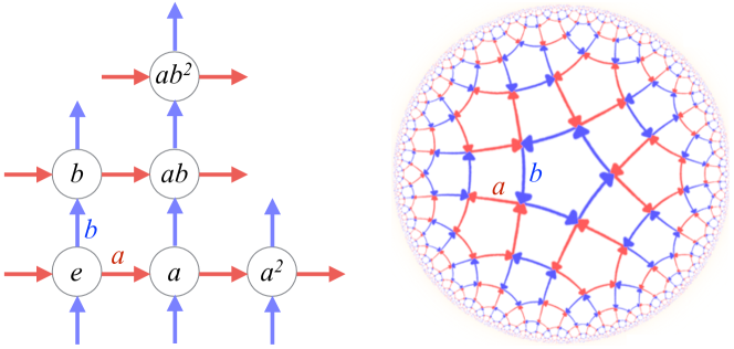
Figure 1: (colors online). Given a group $G$ and a set $S$ of generators, the Cayley graph $\Gamma(G,S)$ is defined as the colored directed graph having set of nodes $G$, set of edges $\{(g,gh);g\in G,h\in S\}$, and a color assigned to each generator $h\in S$. Left: the Cayley graph of the Abelian group $\mathbb{Z}^{2}$ with presentation $\mathbb{Z}^{2}=\langle a,b|aba^{-1}b^{-1}\rangle$, where a and b are two commuting generators. Right: the Cayley graph of the non-Abelian group $G=\langle a,b|a^{5},b^{5},(ab)^{2}\rangle$. The Abelian-group graph is embedded into the Euclidean space $\mathbb{R}^{2}$, the non-Abelian $G$ into the Hyperbolic $\mathbb{H}_{2}$ with (negative) curvature.

The presented setting of QCAs on Cayley graph can lead to field dynamics on both flat spacetime and spacetime with curvature. In the next Section we will focus on the flat case.

IV QCAs on Abelian groups and the small wave-vector limit

In this Section we restrict to the specific subclass of automata whose group $G$ is quasi-isometrically embeddable in the Euclidean space, which is then virtually-Abelian. We also assume that the representation of the isotropy group $L$ in (5) induced by the embedding is orthogonal, which implies that the graph neighborhood is embedded in a sphere. In words, we want homogeneity and isotropy to hold locally also in the embedding space. Our present analysis focus on the Abelian groups $\mathbb{Z}^{d}$ whose Cayley graphs satisfying the isotropic embedding in the Euclidean space $\mathbb{R}^{d}$ are the Bravais lattices. The more general scenario of virtually-Abelian groups is discussed in Section VIII.

In the Abelian case (and also in the virtually-Abelian case as we will discuss in Section VIII) it is possible to describe the automaton in the wave-vector space. Since the group is Abelian we label the group elements by vectors $\mathbf{g}\in\mathbb{Z}^{d}$, and use the additive notation for the group composition, whereas the unitary representation of $\mathbb{Z}^{d}$ on $\ell_{2}(\mathbb{Z}^{d})$ (see Eq. (4)) is expressed as

$$T_{\mathbf{h}}|\mathbf{g}\rangle=|\mathbf{h}+\mathbf{g}\rangle.$$ (8)

Being the group Abelian, we can Fourier transform, and the operator $A$ can be easily block-diagonalized in the wave-vector $\mathbf{k}$ representation as follows

$$A=\int_{B}\operatorname{d}^{3}\!\mathbf{k}\,|{\mathbf{k}}\rangle\langle{\mathbf{k}}|\otimes A_{\mathbf{k}},\qquad A_{\mathbf{k}}:=\sum_{\mathbf{h}\in S}\mathbf{k}\,e^{-i\mathbf{k}\cdot\mathbf{h}}A_{\mathbf{h}},$$ (9)

with $A_{\mathbf{k}}$ unitary for every $\mathbf{k}\in B$, and the vectors $|{\mathbf{k}}\rangle$ given by

$$|\mathbf{k}\rangle:=\frac{1}{\sqrt{|B|}}\sum_{\mathbf{g}\in G}e^{i\mathbf{k}\cdot\mathbf{g}}|\mathbf{g}\rangle.$$ (10)

Notice that due to the discreteness of the lattice the automaton is band-limited in $\mathbf{k}$ with $B$ denoting the first Brillouin zone.

The spectrum $\{e^{i\omega^{(i)}_{\mathbf{k}}}\}$ of the operator $A_{\mathbf{k}}$, or more precisely its dispersion relation that is the expression of the phases $\omega^{(i)}_{\mathbf{k}}$ as functions of $\mathbf{k}$, plays a crucial role in the analysis of the automaton dynamics. Indeed the speed of the wave-front of a plane wave with wave-vector $\mathbf{k}$ is given by the phase-velocity $\omega^{(i)}_{\mathbf{k}}/|\mathbf{k}|$, while the speed of propagation of a narrow-band state having wave-vector $\mathbf{k}$ peaked around the value $\mathbf{k}_{0}$ is given by the group velocity at $\mathbf{k}_{0}$, namely the gradient of the function $\omega^{(i)}_{\mathbf{k}}$ evaluated at $\mathbf{k}_{0}$.

IV.1 The small wave-vector limit

In order be a valid microscopic description of dynamics, the QCA model must recover the usual phenomenology of QFT at the energy scale of the current particle physics experiments, namely the physics of the QCA model and the one of QFT must be the same as far as we restrict to quantum states that cannot probe the discreteness of the underlying lattice. For this reason it is important to address a comparison between the automaton dynamics and the dynamics dictated by the usual QFT differential equations. Here we show how to evaluate the behaviour of an Abelian automaton for small wave-vectors $|\mathbf{k}|\ll 1$, and then discuss a possible approach to a rigorous comparison at different frequency scales.

The physical interpretation of the limit $|\mathbf{k}|\ll 1$ clearly depends on the hypotheses that we make on the order of magnitude of the QCA lattice step and time step. In our approach the QCA is assumed at an hypothetical discrete Planck scale, thus the domain $|\mathbf{k}|\ll 1$ should correspond to the Planckian limit of the automaton. This choice clearly allows one to encompasses the relativistic regime of high energy physics within the small wave-vector limit.

In order to obtain the relativistic limit of an automaton $A_{\mathbf{k}}$ we define its interpolating Hamiltonian $H^{A}(\mathbf{k})$ as the operator satisfying the following equality

$$e^{-iH_{I}^{A}(\mathbf{k})}=X_{\mathbf{k}}.$$ (11)

The term interpolating refers to the fact that the Hamiltonian $H_{I}^{A}(\mathbf{k})$ generates a unitary evolution that interpolates the discrete time determined by the automaton steps through a continuous time $t$ as

$$\psi(\mathbf{k},t)=e^{-iH_{I}^{A}(\mathbf{k})t}\psi(\mathbf{k},0).$$ (12)

However the dynamics provided by the Hamiltonian at the discrete points of the graph is exactly the automaton one.

Now, one can power expand the Hamiltonian of Eq. (12) to first order in $\mathbf{k}$

$$H_{I}^{A}(\mathbf{k})=H_{A}(\mathbf{k})+\mathcal{O}(|\mathbf{k}|^{2}),$$ (13)

which corresponds to the following first-order differential equation

$$i\partial_{t}\psi(\mathbf{k},t)=H_{A}(\mathbf{k})\psi(\mathbf{k},t),$$ (14)

for narrow-band states $\psi(\mathbf{k},t)$ peaked around some $\mathbf{k}_{0}$ with $|\mathbf{k}_{0}|\ll 1$.

The Hamiltonian in Eq. (14) describes the QCA dynamics in the limit of small wave-vectors, and in the next Sections we present QCAs having the Weyl, Dirac and Maxwell Hamiltonian in as such a limit.

In Ref. Bisio et al. (2015b) another more quantitative approach to the QFT limit of a QCA has been presented. Suppose that some automaton $A_{\mathbf{k}}$, (with interpolating Hamiltonian $H^{A}_{I}(\mathbf{k})$) has the unitary $U_{\mathbf{k}}=e^{-iH_{A}(\mathbf{k})}$ (see Eq. (13)) as first-order approximation in $\mathbf{k}$. Then one can set the comparison as a channel discrimination problem and quantify the difference between the two unitary evolutions with the probability of error $p_{e}$ in the discrimination. This probability can be computed as a function of the discrimination experiment parameters—for example the wave-vector and the number of particles and the duration of the evolution— and one can check that for values achievable in current experiments the automaton evolution is undistinguishable from the QFT one. This approach allows us to provide a rigorous proof that, in the limit of input states with vanishing wave-vector, the QCA model recovers free QFT.

V The Weyl automaton

Here we present the unique QCAs on Cayley graphs of $\mathbb{Z}^{d}$, $d=3,2,1$, that satisfy all the requirements of Section II and with minimal internal dimension $s$ for a non-identical evolution (see Ref. D’Ariano and Perinotti (2014) for the detailed derivation).

In any space dimension the only solution for $s=1$ is the identical QCA, which means that it is not possible to have free scalar field automata. The minimal internal dimension for a non-trivial evolution is then $s=2$.

Let us start from the case of dimension $d=3$ that is the most relevant from the physical perspective. For the group $\mathbb{Z}^{3}$ the only Cayley graphs are the primitive cubic (PC) lattice, the body centered cubic (BCC), and the rhombohedral. However only in the BCC case, whose presentation of $\mathbb{Z}^{3}$ involves four vectors $S_{+}=\{\mathbf{h}_{1},\mathbf{h}_{2},\mathbf{h}_{3},\mathbf{h}_{4}\}$ with relator $\mathbf{h}_{1}+\mathbf{h}_{2}+\mathbf{h}_{3}+\mathbf{h}_{4}=0$, one finds solutions satisfying all the assumptions of Section II. There are only four solutions, modulo unitary conjugation, that can be divided in two pairs $A^{\pm}$ and $B^{\pm}$. A pair of solutions is connected to the other pair by transposition in the canonical basis, i.e. $A_{\mathbf{k}}^{\pm}=(B_{\mathbf{k}}^{\pm})^{T}$. The first Brillouin zone $B$ for the BCC lattice is defined in Cartesian coordinates as $-{\sqrt{3}}\pi\leq k_{i}\pm k_{j}\leq{\sqrt{3}}\pi,\,i\neq j\in\{x,y,z\}$ and the solutions in the wave-vector representation are

$$A^{\pm}_{\mathbf{k}}=Iu^{\pm}_{\mathbf{k}}-i\boldsymbol{\sigma}\cdot\tilde{\mathbf{n}}^{\pm}_{\mathbf{k}},\quad B_{\mathbf{k}}^{\pm}=(A_{\mathbf{k}}^{\pm})^{T},$$ (15)

$${\tilde{\mathbf{n}}}^{\pm}_{\mathbf{k}}:=\begin{pmatrix}s_{x}c_{y}c_{z}\mp c_{x}s_{y}s_{z}\\ \mp c_{x}s_{y}c_{z}-s_{x}c_{y}s_{z}\\ c_{x}c_{y}s_{z}\mp s_{x}s_{y}c_{z}\end{pmatrix},\quad u^{\pm}_{\mathbf{k}}:=c_{x}c_{y}c_{z}\pm s_{x}s_{y}s_{z},$$

$$c_{i}:=\cos(k_{i}/\sqrt{3}),\quad s_{i}:=\sin(k_{i}/\sqrt{3}).$$

The matrices $A^{\pm}_{\mathbf{k}}$ and $B^{\pm}_{\mathbf{k}}$ have spectrum $\{e^{-i\omega^{\pm}}_{\mathbf{k}},e^{i\omega^{\pm}}_{\mathbf{k}}\}$ with dispersion relation $\omega^{\pm}_{\mathbf{k}}=\arccos(c_{x}c_{y}c_{z}\mp s_{x}s_{y}s_{z})$ and evolution governed by i) the wave-vector $\mathbf{k}$; ii) the helicity direction $\mathbf{n}^{\pm}_{\mathbf{k}}$; and iii) the group velocity $\mathbf{v}^{\pm}_{\mathbf{k}}:=\nabla_{\mathbf{k}}\omega^{\pm}_{\mathbf{k}}$, which represents the speed of a wave-packet peaked around the central wave-vector $\mathbf{k}$.

The above solutions satisfy the isotropy constraint and are then covariant with respect to the group $L^{\prime}$ of binary rotations around the coordinate axes, with the representation of the group $L^{\prime}$ on $\mathbb{C}^{2}$ given by $\{I,i\sigma_{x},i\sigma_{y},i\sigma_{z}\}$. The group $L^{\prime}$ is transitive on the four BCC generators of $S_{+}$.

In dimension $d=2$, the only inequivalent Cayley graphs of $\mathbb{Z}^{2}$ are the square lattice and the hexagonal lattice. Also for $d=2$ we have solutions only on one of the possible Cayley graphs, the square lattice, whose presentation of $\mathbb{Z}^{2}$ involves two vectors $S_{+}=\{\mathbf{h}_{1},\mathbf{h}_{2}\}$. The first Brillouin zone $B$ in this case is given by $\sqrt{2}\pi\leq k_{i}\leq\sqrt{2}\pi,\,i\in\{x,y\}$ and there are only two solutions modulo unitary conjugation,

$$A_{\mathbf{k}}=Iu_{\mathbf{k}}-i\boldsymbol{\sigma}\cdot\tilde{\mathbf{n}}_{\mathbf{k}},\quad B_{\mathbf{k}}:=A_{\mathbf{k}}^{T},$$ (16)

$$\tilde{\mathbf{n}}_{\mathbf{k}}:=\begin{pmatrix}s_{x}c_{y}\\ c_{x}s_{y}\\ s_{x}s_{y}\end{pmatrix},\quad u_{\mathbf{k}}:=c_{x}c_{y},\qquad c_{i}:=\cos(k_{i}/\sqrt{2}),\quad s_{i}:=\sin(k_{i}/\sqrt{2}),$$

with dispersion relation $\omega_{\mathbf{k}}=\arccos(c_{x}c_{y})$.

The QCA in Eq. (LABEL:eq:weyl2d) is covariant for the cyclic transitive group generated by the transformation that exchanges $\mathbf{h}_{1}$ and $\mathbf{h}_{2}$, with representation given by the rotation by $\pi$ around the $x$-axis. Since the isotropy group has a reducible representation, the most general automaton is actually given by $(\cos\theta I+i\sin\theta\sigma_{x})A_{\mathbf{k}}$.

Finally for $d=1$ the unique Cayley graph satisfying our requirements for $\mathbb{Z}$ is the lattice $\mathbb{Z}$ itself, presented as the free Abelian group on one generator $S_{+}=\{h\}$. From the unitarity conditions one gets the unique solution

$$A_{k}=u_{\mathbf{k}}I-i\boldsymbol{\sigma}\cdot\tilde{\mathbf{n}}_{\mathbf{k}},\qquad\tilde{\mathbf{n}}_{\mathbf{k}}:=\begin{pmatrix}0\\ 0\\ \sin k\end{pmatrix},\quad u_{\mathbf{k}}:=\cos k,$$ (17)

with dispersion relation $\omega_{k}=k$.

We call the solutions (15), (LABEL:eq:weyl2d) and (17) Weyl automata, because in the limit of small wave-vectors of Section IV.1 their evolution obeys Weyl’s equation in space dimension $d=3$, $d=2$ and $d=1$, respectively. Any solution in dimension $d$ is of the form

$$W_{\mathbf{k}}=u_{\mathbf{k}}I-i\boldsymbol{\sigma}\cdot\tilde{\mathbf{n}}_{\mathbf{k}},$$ (18)

for certain $u_{k}$ and $\mathbf{n}_{k}$ (see Eqs. (15), (LABEL:eq:weyl2d) and (17) fro $d=3,2,1$) and has dispersion relation

$$\omega_{\mathbf{k}}=\arccos{u_{\mathbf{k}}}.$$ (19)

It is easily to check that the interpolating Hamiltonian is

$$H^{W}_{I}(\mathbf{k})=\boldsymbol{\sigma}\cdot\mathbf{n}_{\mathbf{k}},\qquad\mathbf{n}_{\mathbf{k}}:=\frac{\omega_{\mathbf{k}}}{\sin\omega_{\mathbf{k}}}\tilde{\mathbf{n}}_{\mathbf{k}},$$ (20)

and by power expanding at the first order in $\mathbf{k}$ one has

$$H_{I}^{W}=H_{W}(\mathbf{k})+\mathcal{O}(|\mathbf{k}|^{2}),\qquad H_{W}(\mathbf{k})=\tfrac{1}{\sqrt{d}}\boldsymbol{\sigma}\cdot\mathbf{k}$$ (21)

where $H_{W}(\mathbf{k})$ coincides with the usual Weyl Hamiltonian in $d$ dimensions once the wave-vector $\mathbf{k}$ is interpreted as the momentum.

VI The Dirac automaton

From the previous section we know that in our framework all the admissible QCAs with $s=2$ give the Weyl equation in the limit of small wave-vectors. In order to get a more general dynamics—say the Dirac one—it is then necessary to increase the internal degree of freedom $s$. Instead of deriving the most general QCAs with $s>2$. in Ref. D’Ariano and Perinotti (2014) is shown how the Dirac limit is obtained from the local coupling of two Weyl automata in any space dimension $d=1,2,3$. Here we shortly review this result.

Starting from two arbitrary Weyl automata $W$ and $W^{\prime}$ in dimension $d$ (see the solutions (15), (LABEL:eq:weyl2d) and (17) in for $d=3$, $d=3$ and $d=1$, respectively), the coupling is obtained by performing the direct-sum of their representatives $W_{\mathbf{k}}$ and ${W^{\prime}_{\mathbf{k}}}$, obtaining a QCA with $s=4$, and introducing off-diagonal blocks $X$ and $Y$ in such a way that the obtained matrix is unitary. The locality of the coupling implies that the off-diagonal blocks are independent of $\mathbf{k}$, namely

$$D_{\mathbf{k}}:=\begin{pmatrix}p{W_{\mathbf{k}}}&qX\\ rY&t{W^{\prime}_{\mathbf{k}}}\end{pmatrix},\qquad p,q,r,t\in\mathbb{C}.$$ (22)

In order to satisfy all the hypothesis of Section II it is possible to show that the unique local coupling of Weyl QCAs, modulo unitary conjugation, are

$$D_{\mathbf{k}}:=\begin{pmatrix}nW_{\mathbf{k}}&im\\ im&nW_{\mathbf{k}}\end{pmatrix},\qquad n,m\in\mathbb{R}^{+},\quad n^{2}+m^{2}=1,$$ (23)

which are conveniently expressed in terms of gamma matrices in the spinorial representation as follows

$$D_{\mathbf{k}}:=nIu_{\mathbf{k}}-in\gamma^{0}\boldsymbol{\gamma}\cdot\tilde{\mathbf{n}}_{\mathbf{k}}+im\gamma^{0},$$ (24)

where the functions $u_{\mathbf{k}}$ and $\tilde{\mathbf{n}}_{\mathbf{k}}$ depends on the chosen $d$ dimension Weyl automaton $W$ in Eq. (23). Notice the dispersion relation of the QCAs (24) that is simply given by

$$\omega_{\mathbf{k}}=\arccos[\sqrt{1-m^{2}}u_{\mathbf{k}}].$$ (25)

The QCAs in Eq. (23) are denoted Dirac QCAs because in the small wave-vector limit narrow-band states $\psi(\mathbf{k},t)$ with $|\mathbf{k}|\ll 1$ evolves according to the usual Dirac equation. The interpolating Hamiltonian $H_{I}^{D}(\mathbf{k})$ is given by

$$H_{I}^{D}(\mathbf{k})=f(\mathbf{k})(n\gamma^{0}\boldsymbol{\gamma}\cdot\tilde{\mathbf{n}}_{\mathbf{k}}-m\gamma^{0}),\qquad f(\mathbf{k}):=\frac{\omega_{\mathbf{k}}}{\sin\omega_{\mathbf{k}}},$$ (26)

that by power expanding at the first order in $\mathbf{k}$ is approximated as follows

$$H_{I}^{D}(\mathbf{k})=H_{D}(\mathbf{k})+\mathcal{O}(|\mathbf{k}|^{2}),\qquad H_{D}(\mathbf{k})=\frac{n}{\sqrt{d}}\gamma^{0}\boldsymbol{\gamma}\cdot\mathbf{k}+m\gamma^{0}.$$ (27)

Finally, for small values of $m$, $m\ll 1$, we have $n\simeq 1+\mathcal{O}(m^{2})$ and neglecting terms of order $\mathcal{O}(m^{2})$ and $\mathcal{O}(|\mathbf{k}|^{2})$

$$H_{I}^{D}(\mathbf{k})=\frac{1}{\sqrt{d}}\gamma^{0}\boldsymbol{\gamma}\cdot\mathbf{k}+m\gamma^{0}+O(m^{2})+O(|\mathbf{k}|^{2}),$$ (28)

one has the Dirac Hamiltonian with the wave-vector $\mathbf{k}$ and the parameter $m$ interpreted as momentum and mass, respectively.

It is interesting to notice that in $d=1$, modulo a permutation of the canonical basis, the Dirac QCA corresponds to two identical and decoupled $s=2$ automata. Each of these QCAs coincide with the one dimensional Dirac automaton derived in Ref. Bisio et al. (2015b). The last one was derived as the simplest ($s=2$) homogeneous QCA covariant with respect to the parity and the time-reversal transformation, which are less restrictive than isotropy that singles out the only Weyl QCA (17) in one space dimension.

VII QCA for free electrodynamics

In Sections V and VI we showed how the dynamics of free Fermionic fields can be derived within the QCA framework starting from informational principles. Within this perspective the information contained in a finite number of systems must be finite and this is the reason why at the site of the lattices we put Fermionic modes. We now show that the same framework can also accomodate a QCA model for the free electromagnetic field and thus for Bosonic quantum fields with the canonical commutation relation recovered as approximated by many Fermionic modes. The material presented in this Section is a review of Ref. Bisio et al. (2014) where we refer for a complete presentation.

The basic idea behind this approach is to model the photon as a correlated pair of Fermions evolving according to the Weyl QCA presented in Section V. Then we show that in a suitable regime both the free Maxwell equation in three dimensions and the Bosonic commutation relation are recovered. Let us then consider a couple of two component Fermionic fields, which in the wave-vector representation are denoted as $\psi(\mathbf{k})$ and $\varphi(\mathbf{k})$. The evolutions of these two fields are given by

$${\psi}(\mathbf{k},t+1)=W_{\mathbf{k}}{\psi}(\mathbf{k},t).\quad{\varphi}(\mathbf{k},t+1)=W_{\mathbf{k}}^{*}{\varphi}(\mathbf{k},t).$$ (29)

Where the matrix $W_{\mathbf{k}}$ can be any of the Weyl QCAs in three space dimensions of Eq. (15), (the whole derivation is independent on this choice) and $W_{\mathbf{k}}^{*}$ denotes the complex conjugate matrix.

We now introduce the following bilinear operators

$$\mathbf{G}_{T}(\mathbf{k},t) :=\mathbf{G}(\mathbf{k},t)-\left(\frac{\mathbf{n}_{\frac{\mathbf{k}}{2}}}{|\mathbf{n}_{\frac{\mathbf{k}}{2}}|}\cdot{\mathbf{G}}(\mathbf{k},t)\right)\frac{\mathbf{n}_{\frac{\mathbf{k}}{2}}}{|\mathbf{n}_{\frac{\mathbf{k}}{2}}|}$$ (30)

$$\mathbf{G}(\mathbf{k},t) :=(G^{1}(\mathbf{k},t),G^{2}(\mathbf{k},t),G^{3}(\mathbf{k},t))^{T}$$

$$G^{i}(\mathbf{k},t) :=\varphi^{T}(\tfrac{\mathbf{k}}{2},t)\sigma^{i}\psi(\tfrac{\mathbf{k}}{2},t)=\varphi^{T}(\mathbf{k},0)(W_{\tfrac{\mathbf{k}}{2}}^{\dagger}\sigma^{i}W_{\tfrac{\mathbf{k}}{2}})\psi(\tfrac{\mathbf{k}}{2},0)$$

with $\mathbf{n}_{\mathbf{k}}$ as in Eq. (V). By construction the field $\mathbf{G}_{T}(\mathbf{k},t)$ obeys

$$\mathbf{n}_{\frac{\mathbf{k}}{2}}\cdot\mathbf{G}_{T}(\mathbf{k},t) =0,$$ (31)

$$\mathbf{G}_{T}(\mathbf{k},t) =\operatorname{Exp}(-i2\mathbf{n}_{\tfrac{\mathbf{k}}{2}}\cdot\mathbf{J}t)\mathbf{G}_{T}(\mathbf{k},0)$$ (32)

where we used the identity $\exp(-\tfrac{i}{2}\mathbf{v}\cdot\boldsymbol{\sigma})\boldsymbol{\sigma}\exp(\tfrac{i}{2}\mathbf{v}\cdot\boldsymbol{\sigma})=\operatorname{Exp}(-i\mathbf{v}\cdot\mathbf{J})\boldsymbol{\sigma}$ where the matrix $\operatorname{Exp}(-i\mathbf{v}\cdot\mathbf{J})$ acts on $\boldsymbol{\sigma}$ regarded as a vector and $\mathbf{J}=(J_{x},J_{y},J_{z})$ is the vector of angular momentum operators. Taking the time derivative of Eq. (32) we obtain

$$\partial_{t}\mathbf{G}_{T}(\mathbf{k},t)=2\mathbf{n}_{\tfrac{\mathbf{k}}{2}}\times\mathbf{G}_{T}(\mathbf{k},t).$$ (33)

If $\mathbf{E}_{G}$ and $\mathbf{B}_{G}$ are two Hermitian operators defined by the relation

$$\mathbf{E}_{G}:=|{\mathbf{n}}_{\tfrac{\mathbf{k}}{2}}|(\mathbf{G}_{T}+\mathbf{G}_{T}^{\dagger}),\quad\mathbf{B}_{G}:=i|{\mathbf{n}}_{\tfrac{\mathbf{k}}{2}}|(\mathbf{G}_{T}^{\dagger}-\mathbf{G}_{T}),$$ (34)

then Eq. (31) and Eq. (33) can be rewritten as

$$\begin{aligned} 2\mathbf{n}_{\tfrac{\mathbf{k}}{2}}\cdot\mathbf{E}_{G}&=0&2\mathbf{n}_{\tfrac{\mathbf{k}}{2}}\cdot\mathbf{B}_{G}&=0\\ \partial_{t}\mathbf{E}_{G}&=i2\mathbf{n}_{\tfrac{\mathbf{k}}{2}}\times\mathbf{B}_{T}(\mathbf{k},t)&\partial_{t}\mathbf{B}_{G}&=-i2\mathbf{n}_{\tfrac{\mathbf{k}}{2}}\times\mathbf{E}_{T}(\mathbf{k},t)\end{aligned}$$ (35)

that are the free Maxwell’s equation in the wave-vector space with the substitution $2\mathbf{n}_{\tfrac{\mathbf{k}}{2}}\to\mathbf{k}$. In the limit $|\mathbf{k}|\ll 1$ one has $2\mathbf{n}_{\tfrac{\mathbf{k}}{2}}\sim\mathbf{k}$ and the usual free electrodynamics is recovered.

However the field as defined in Eqs. (30) and (34) does not allow to recover the correct Bosonic commutation relation. As shown in Ref. Bisio et al. (2014) the solution to this problem is to replace the operators $G^{i}$ defined in Eq. (30) with the operators $F^{i}$ defined as

$$F^{i}(\mathbf{k}):=\int\frac{d\mathbf{q}}{(2\pi)^{3}}f_{\mathbf{k}}(\mathbf{q})\varphi\left(\tfrac{\mathbf{k}}{2}-\mathbf{q}\right)\sigma^{i}\psi\left(\tfrac{\mathbf{k}}{2}+\mathbf{q}\right)$$ (36)

where $\int\frac{d\mathbf{q}}{(2\pi)^{3}}|f_{\mathbf{k}}(\mathbf{q})|^{2}=1,\forall\mathbf{k}$. In terms of $\mathbf{F}(\mathbf{k})$, we can define the polarization operators $\gamma^{i}(\mathbf{k})$ of the electromagnetic field as follows

$$\gamma^{i}(\mathbf{k}):=\mathbf{u}^{i}_{\mathbf{k}}\cdot\mathbf{F}(\mathbf{k},0),\quad i=1,2,$$ (37)

$$\mathbf{u}^{i}_{\mathbf{k}}\cdot\mathbf{n}_{\mathbf{k}}=\mathbf{u}^{1}_{\mathbf{k}}\cdot\mathbf{u}^{2}_{\mathbf{k}}=0,\;|\mathbf{u}^{i}_{\mathbf{k}}|=1,\;(\mathbf{u}^{1}_{\mathbf{k}}\times\mathbf{u}^{2}_{\mathbf{k}})\cdot\mathbf{n}_{\mathbf{k}}>0.$$ (38)

In order to avoid the technicalities of the continuum we suppose to have a discrete wave-vector space (as if the electromagnetic field were confined in a finite volume) and moreover let us assume $|{f}_{\mathbf{k}}(\mathbf{q})|^{2}$ to be a constant function over a region $\Omega_{\mathbf{k}}$ which contains $N_{\mathbf{k}}$ modes, i.e. $|{f}_{\mathbf{k}}(\mathbf{q})|^{2}=\tfrac{1}{N_{\mathbf{k}}}$ if $\mathbf{q}\in\Omega_{\mathbf{k}}$ and $|{f}_{\mathbf{k}}(\mathbf{q})|^{2}=0$ if $\mathbf{q}\not\in\Omega_{\mathbf{k}}$. Then, for a given state $\rho$ of the field we denote by $M_{\varphi,\mathbf{k}}$ (resp. $M_{\psi,\mathbf{k}}$) the mean number of type $\varphi$ (resp $\psi$) Fermion in the region $\Omega_{\mathbf{k}}$. One can then show that, for states such that $M_{\xi,\mathbf{k}}/N_{\mathbf{k}}\leq\varepsilon$ for all $\xi=\varphi,\psi$ and $\mathbf{k}$ and for $\varepsilon\ll 1$ we can safely assume $[\gamma^{i}(\mathbf{k}),{\gamma^{j}}^{\dagger}(\mathbf{k}^{\prime})]_{-}=\delta_{i,j}\delta_{\mathbf{k},\mathbf{k}^{\prime}}$, i.e. the polarization operators are Bosonic operators.

VIII Future perspectives: non-Abelian Cayley graphs and tiling

In Section II we have shown how from a denumerable set of unitarily an linearly interacting systems, the locality and homogeneity of the interactions lead to the structure of the Cayley graph of some group $G$, with vertices corresponding to the set of systems and edges corresponding to couples of interacting systems.

Then, we further restricted our scenario assuming the isotropy, the equivalence of the directions on the graph, and the Abelianity of the group $G$. Within this perspective all possible QCAs having minimal internal degree of freedom $s=2$ for a non trivial evolution have been derived in Section V and give the usual Weyl dynamics in the limit of small wave-vector. Using the Weyl QCAs, in Sections VI and VII we constructed other simple automata, recovering the Dirac and the Maxwell equation in the small wave-vector regime.

Keeping locality and homogeneity one could study automata defined on arbitrary Cayley graphs, relaxing the hypothesis of isotropy and Abelianity. A very general procedure that can be defined is the tiling. Suppose to have a QCA $A$ with internal Hilbert space $\mathbb{C}^{s}$ on the Cayley graph $\Gamma(G,S)$ of some group $G$. Whenever a group $G$ has a subgroup $G^{\prime}\subset G$ of finite index $r$ it is possible to describe the same automaton $A$ as an automaton $A^{\prime}$ on a Cayley graph $\Gamma(G^{\prime},S^{\prime})$ of $G^{\prime}$ and with bigger internal system $\mathbb{C}^{sr}$. Intuitively the information on the cosets is included in the internal degree of freedom and the map performing this “inclusion” is the unitary map $U:\ell_{2}(G)\otimes\mathbb{C}^{s}\rightarrow\ell_{2}(G^{\prime})\otimes\mathbb{C}^{sr}$ given by

$$U:=\sum_{i=1}^{r}\sum\limits_{\mathbf{g}^{\prime}\in G^{\prime}}|\mathbf{g}^{\prime}\rangle|i\rangle\langle c_{i}\mathbf{g}^{\prime}|\otimes I_{s},$$ (39)

where $\{c_{1},\ldots,c_{r}\}$ are the representatives of the $r$ cosets.

As a first application, the tiling allows for the wave-vector space description of any QCA on a group $G$ quasi-isometrically embeddable in $\mathbb{R}^{n}$. As already stated in Section III these groups are the virtually-Abelian ones, therefore they admit a finite index Abelian subgroup $G^{\prime}\subset G$, and using the tiling a QCA over $G$ can be regarded as a QCA on the Abelian subgroup $G^{\prime}$.

A second application is the construction of QCAs starting from the tiling of simpler automata. The main motivation for this is in the difficulty of solving the unitarity constraint in Eq. (6) for large matrices. The easiest situation is that of scalar QCAs where the transition matrices are simply complex numbers. While in the Abelian case scalar QCAs with a non trivial evolution are not admissible, in a more general scenario scalar solutions can be found Acevedo et al. (2008). Within this perspective one could explore the emergence spinorial QCAs from the tiling of scalar automata on non-Abelian groups.