Spectral-Efficiency Analysis of Massive MIMO Systems in Centralized and Distributed Schemes

Abstract

This paper analyzes the spectral efficiency of massive multiple-input multiple-output (MIMO) systems in both centralized and distributed configurations, referred to as C-MIMO and D-MIMO, respectively. By accounting for real environmental parameters and antenna characteristics, namely, path loss, shadowing effect, multi-path fading and antenna correlation, a novel comprehensive channel model is first proposed in closed-form, which is applicable to both types of MIMO schemes. Then, based on the proposed model, the asymptotic behavior of the spectral efficiency of the MIMO channel under both the centralized and distributed configurations is analyzed and compared in exact forms, by exploiting the theory of very long random vectors. Afterwards, a case study is performed by applying the obtained results into MIMO networks with circular coverage. In such a case, it is attested that for the D-MIMO of cell radius $r_{\mathrm{c}}$ and circular antenna array of radius $r_{\mathrm{a}}$, the optimal value of $r_{\mathrm{a}}$ that maximizes the average spectral efficiency is accurately established by $r_{\mathrm{a}}^{\mathrm{opt}}=r_{\mathrm{c}}/1.31$. Monte Carlo simulation results corroborate the developed spectral-efficiency analysis.

I Introduction

Massive MIMO communication technique, where tens or a few hundred antennas are deployed at either or both ends of a wireless link, promises significant performance gains in terms of spectral efficiency, energy efficiency, security and reliability compared with conventional MIMO [1], and is becoming a cornerstone of future 5G systems [2]. To implement massive MIMO in wireless networks, two different schemes can be adopted (see, e.g., [3, 4, 5]): centralized (C-MIMO), where antennas are co-located at both the transmit (Tx) and the receive (Rx) sides as illustrated in Fig. 1-a (which is essentially equivalent to conventional MIMO system), and distributed (D-MIMO), where base station (BS) antennas are deployed at different geographical locations while connected together through high-capacity backhaul links such as fibre-optic cables, as shown in Fig. 1-b.

From a practical point of view, C-MIMO is more easy to mathematically analyze and physically deploy, compared with D-MIMO. In fact, unlike the former, the latter suffers from different degrees of path losses caused by different access distances to different distributed antennas, which makes the performance analysis and design more challenging. Also, since the location of antennas in D-MIMO has a significant effect on the system performance, optimization of the antenna locations is crucial [6, 4]. This task may become very challenging because of the large numbers (massive) of Tx/Rx antennas. On the other hand, in practice, arbitrary antenna locations or optimal topology may lead to a prohibitive cost for the backhaul component, as well as installation cost for the distributed setting.

D-MIMO technique, however, exhibits several advantages compared with C-MIMO, such as lower transmit power, higher multiplexing gain, higher spectral efficiency, enhanced coverage area and ease of network planning [7, 8]. As such, both C-MIMO and D-MIMO represent promising choices for practical implementation of massive MIMO technique, each depending on potentially preferable criteria mentioned above.

No matter whether the centralized or distributed configuration is concerned, to capture the propagation characteristics and to understand the system performance and behaviour in real physical environments, two fundamental tasks are to i) develop an analytical channel model, where path loss, shadowing effect and multi-path fading are accounted for; and to ii) conduct analytical performance evaluation and assess key factors that determine system performance. In particular, for D-MIMO systems, different path losses and shadowing effects w.r.t. different BS antennas are critical to the realization of Tx/Rx diversity. In addition, antenna correlation is inherent to the realization of massive MIMO, because of the lack of sufficient physical space to separate the large number of antennas in case they are co-located.

In practice, the performance of point-to-point massive MIMO serves as a benchmark for further performance evaluation in multi-user settings. Also, point-to-point massive MIMO finds wide applications, e.g., high-speed wireless backhaul link between BSs [9]. However, despite the extreme importance of point-to-point massive MIMO, there is no existing work that successfully accounts for all the aforementioned parameters (i.e., path loss, shadowing effect, multi-path fading and antenna correlation), while developing channel model and conducting closed-form performance analysis. In particular, it was shown in [10] that for MIMO channels, the spectral efficiency grows linearly with the minimum between the numbers of Tx and Rx antennas, even if they tend to infinity. The asymptotic result when the number of antennas at only one side goes to infinity was reported in [11, 12]. In [10, 11, 12], only basic multi-path fading was considered whereas path loss, shadowing and antenna correlation were ignored. In [13, 14, 15], the capacity of correlated multi-antenna channels was studied, in both regimes of finite numbers of antennas (in [13]) and large numbers of antennas (in [13, 14, 15]), where only the Rayleigh fading and the antenna correlation were considered. Recently, in [16] and its companion conference version [17], a comprehensive channel model consisting of path loss, shadowing, multi-path fading, antenna correlation and polarization was firstly developed. Then, an upper bound on the ergodic capacity of point-to-point C-MIMO was derived, by using the Hadamard’s determinant inequality, and further asymptotically analyzed in the sense of larger number of Tx and/or Rx antennas.

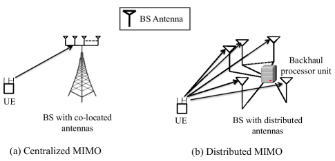
Figure 1: Two configurations of point-to-point massive MIMO systems: (a) C-MIMO, where antennas are co-located at the BS and the UE sides and, thus, distances from UE to BS antennas are almost identical; (b) D-MIMO, where BS antennas are deployed at different geographical locations while connected together through the backhaul processor unit, implying that the distances from UE to BS antennas are different.

Compared to our previous work [16, 17], the major contributions of this paper are summarized as follows.

1) This paper develops a general channel model suitable for both massive C-MIMO and D-MIMO, where major environmental parameters and antenna physical parameters are accounted for. As apposed to the Kronecker correlation model used in [17], this paper uses the Weichselberger model which is more accurate than the former (as detailed later in Section II-B). Moreover, although various parameters needed in channel modeling have been partially considered to some extent in the open literature, key channel parameters, namely, path loss, shadowing, multi-path fading and antenna correlation, are concurrently taken into account and their effects on spectral efficiency are investigated in this paper.

2) The asymptotic behavior of the spectral efficiency of C-MIMO and D-MIMO is analyzed, in the sense of large number of Rx antennas. More specifically:

1. We first extend the law of large numbers for very long random vectors with independent but not necessarily identically distributed (i.n.i.d.) entries, to the more general case of very long random vectors with weighted i.n.i.d. entries, where a condition is imposed onto the weights to guarantee the convergence in probability.

2. Then, two target matrices are introduced in the expressions of the spectral efficiency: $\mathbf{M}_{\mathrm{C}}$ for C-MIMO and $\mathbf{M}_{\mathrm{D}}$ for D-MIMO. Afterwards, the above results on the law of large numbers for very long random vectors with weighted i.n.i.d. entries are exploited to derive the asymptotic expressions of the entries of $\mathbf{M}_{\mathrm{C}}$ and of $\mathbf{M}_{\mathrm{D}}$, w.r.t. the number of Rx antennas $N_{R}$ where $N_{R}\to\infty$.

3. The resulting asymptotic behavior is then applied to derive the intended spectral efficiency, yielding novel expressions from which new insights into the system performance can be gained. In particular, our results show that, i) D-MIMO does not always outperform C-MIMO in terms of spectral efficiency; ii) D-MIMO exhibits a higher multiplexing gain than that of C-MIMO, up to $N_{T}\times N_{R}$ where $N_{T}$ denotes the number of Tx antennas; and iii) the performance of massive MIMO on the uplink is mainly determined by the correlation characteristics at the Tx side instead of the Rx side, given that the Weichselberger correlation model is applied.

3) A case study is performed by applying the obtained results in a pertinent scenario where D-MIMO adopts a circular topology, and several key insights into the system performance and optimal antenna deployment are gained. In particular, it is demonstrated that for D-MIMO with circular topology of cell radius $r_{\mathrm{c}}$ and circular antenna array of radius $r_{\mathrm{a}}$, the optimal value of $r_{\mathrm{a}}$ that maximizes the average spectral efficiency is given by $r_{\mathrm{a}}^{\mathrm{opt}}=r_{\mathrm{c}}/1.31$.

To detail the aforementioned contributions, the following content of the paper is organized as follows. Section II develops the channel model suitable for both C-MIMO and D-MIMO, and Section III derives the associated asymptotic spectral efficiency. Afterwards, the case study is conducted in Section IV. Section V presents numerical results pertaining to the developed analyses, in comparison with Monte Carlo simulation results. Section VI concludes the paper and, finally, some detailed derivations are relegated to appendices.

Notation: In the paper, scalars are represented by lowercase letters like $h$, whereas vectors and matrices are represented by bold lowercase and uppercase letters, like $\mathbf{h}$ and $\mathbf{H}$, respectively. The row vector $\mathbf{h}$ with size $n$ is written as $\mathbf{h}=[h_{1},h_{2},\cdots,h_{n}]$ and the $(i,j)^{\mathrm{th}}$ entry of $\mathbf{H}$ is denoted by $[\mathbf{H}]_{i,j}$. The subscript $n\times m$ in $\mathbf{A}_{n\times m}$ means the size of $\mathbf{A}$, i.e., $\mathbf{A}\in\mathcal{C}^{n\times m}$. $\mathbf{1}_{n}$ refers to the $n\times 1$ column vector with all entries being unity, and $\mathbf{I}_{n}$ denotes the identity matrix of size $n\times n$. Operators $(.)^{\rm T}$, $(.)^{\rm H}$, $\det(.)$ and $\odot$ refer to the transpose, Hermitian transpose, determinant and Hadamard product, respectively. $\mathrm{Pr}(.)$, $\mathbb{E}\{.\}$ and $\mathrm{Var}\{.\}$ stand for mathematical probability, expectation and variance, respectively.

II Massive MIMO System and Channel Modeling

II-A System Models of C-MIMO and D-MIMO

We consider the uplink of a multi-user massive MIMO system, where the BS is equipped with $N_{R}$ Rx antennas while each user equipment (UE) is equipped with $N_{T}$ Tx antennas. In the centralized setting as illustrated in Fig. 1-a, the $N_{R}$ antennas of the BS are co-located, whereas in the distributed scheme shown in Fig. 1-b, the $N_{R}$ antennas of the BS are separately distributed in geography. In both settings, it is assumed that the number of antennas at the BS is large, i.e., the value of $N_{R}$ is on the order of tens or even hundreds, and that $N_{R}>N_{T}$ since the number of Tx antennas at UE is usually not large due to the physical size limitations. Since this paper focuses on a comprehensive channel model used for the system performance analysis, it is assumed that there is no hardware imperfections at the BS antenna array. Further, it is assumed that in the D-MIMO scheme, high-capacity backhaul links such as fibre-optic cables connect the BS antennas, which cooperate perfectly with each other [4, 5].

II-B Channel Models

In both C-MIMO and D-MIMO systems, the physical channel between both ends of any communication link is assumed to be subject to path loss, shadowing and multi-path fading. In the centralized scheme, the path-loss components on the radio link between the UE antennas and the BS antennas are independent and identically distributed (i.i.d.), since in this setting, antennas at either end (transmitter or receiver) are at the same location. In the distributed scheme, on the other hand, since different BS antennas are deployed at different geographical locations, the path-loss components of radio links between the UE and the antennas of the BS are i.n.i.d.. With the system model described above, a channel model applicable to both C-MIMO and D-MIMO systems, $\mathbf{H}\in\mathcal{C}^{N_{R}\times N_{T}}$, can be explicitly given by

$$\mathbf{H}=\mathbf{D}^{\frac{1}{2}}\mathbf{H}_{0},$$ (1)

where $\mathbf{H}_{0}\in\mathcal{C}^{N_{R}\times N_{T}}$ models multi-path fading while $\mathbf{D}\in\mathcal{R}^{N_{R}\times N_{R}}$ represents path loss and shadowing effect. With the observations right before (1), it is readily shown that $\mathbf{D}$ in (1) is a diagonal matrix given by

$$\mathbf{D}= d^{-\nu}\varphi\,\mathbf{I}_{N_{R}},$$ ; (2)

$$\mathbf{D}= \mathrm{diag}\left\{d_{i}^{-\nu}{\varphi}_{i}\right\}_{i=1}^{N_{R}},$$ , (3)

where in (2), $d$ and $\varphi$ denote the Euclidean distance and the shadowing effect pertaining to the link between the UE and the BS of a C-MIMO system, respectively; and where in (3), $d_{i}$ and $\varphi_{i}$ refer to the Euclidean distance and the shadowing effect pertaining to the link between the UE and the $i^{\mathrm{th}}$ BS antenna of a D-MIMO system, for all $i\in\{1,2,\ldots,N_{R}\}$. In (2) and (3), $\nu>2$ is the path-loss exponent. By using a similar methodology as detailed in [17, Sec. II.A], $\varphi$ shown in (2) can be well described by a Gamma distribution. Accordingly, the probability density function (PDF) of $\varphi$ can be written as

$$f_{\varphi}(x)=\frac{1}{\Gamma(\alpha)}\left(\frac{\alpha}{\Omega}\right)^{\alpha}x^{\alpha-1}\exp{\left(-\frac{\alpha}{\Omega}x\right)},$$ (4)

where $\Gamma(x)=\int_{0}^{x}{{t^{x-1}e^{-t}}\,\mathrm{d}t}$ denotes the Gamma function, $\alpha>0.5$ inversely reflects the shadowing severity and $\Omega$ is the average power of the shadowing effect. For the sake of brevity, the Gamma distribution in the form of (4) is shortly denoted $\mathcal{G}(\alpha,\Omega/\alpha)$, with $\alpha$ and $\Omega/\alpha$ being the shape parameter and the scaling factor, respectively. Accordingly, $\varphi_{i}$ shown in (3) is distributed according to

$$f_{\varphi_{i}}(y)=\mathcal{G}\left(\alpha_{i},\frac{\Omega}{\alpha_{i}}\right),$$ (5)

where $\alpha_{i}$ denotes the shadowing parameter pertaining to the link between the UE and the $i^{\mathrm{th}}$ BS antenna, for all $i\in\{1,2,\ldots,N_{R}\}$.

If antenna correlation at the Tx and Rx sides is considered and modelled by the well-known Kronecker model, namely,

$$\mathbf{H}_{0}\triangleq\mathbf{\Theta}_{R}^{\frac{1}{2}}\,\widehat{\mathbf{H}}\left(\mathbf{\Theta}_{T}^{\frac{1}{2}}\right)^{\rm H},$$ (6)

where $\mathbf{\Theta}_{T}\in\mathcal{C}^{N_{T}\times N_{T}}$ and $\mathbf{\Theta}_{R}\in\mathcal{C}^{N_{R}\times N_{R}}$ refer to the correlation matrices at the transmitter and the receiver, respectively; and where the $(i,j)^{\mathrm{th}}$ entry of matrix $\widehat{\mathbf{H}}$, for all $i\in\{1,2,\ldots,N_{R}\}$ and $j\in\{1,2,\ldots,N_{T}\}$, follows a circularly symmetric complex Gaussian (CSCG) distribution:

$$[\widehat{\mathbf{H}}]_{i,j}\sim\mathcal{CN}(0,1),$$ (7)

then, substituting (2), (3) and (6) into (1) yields the channel model

$$\mathbf{H}= d^{-\frac{\nu}{2}}{\varphi}^{\frac{1}{2}}\,\mathbf{\Theta}_{R}^{\frac{1}{2}}\,\widehat{\mathbf{H}}\left(\mathbf{\Theta}_{T}^{\frac{1}{2}}\right)^{\rm H},$$ ; (8)

$$\mathbf{H}= \mathrm{diag}\left\{d_{i}^{-\frac{\nu}{2}}{\varphi}_{i}^{\frac{1}{2}}\right\}_{i=1}^{N_{R}}\,\widehat{\mathbf{H}}\,\left(\mathbf{\Theta}_{T}^{\frac{1}{2}}\right)^{\rm H},$$ . (9)

It is noted that $\mathbf{\Theta}_{R}$ in (8) denotes the correlation matrix at the Rx antennas in the C-MIMO scheme. As far as D-MIMO is concerned, however, Rx antennas at BS are well separated in geography and, thus, correlation between them is negligible. Accordingly, $\mathbf{\Theta}_{R}$ in (8) reduces to an identity matrix in the D-MIMO scheme, as implied by (9).

By recalling the exponential correlation model widely used between antenna elements [18, 19], the entries of $\mathbf{\Theta}_{R}$ and $\mathbf{\Theta}_{T}$ in the model above can be explicitly given by

$$[\mathbf{\Theta}_{I}]_{k,l}={\theta}_{I}^{|k-l|},~{}\forall k,l\in\left\{1,2,\cdots,N_{I}\right\},$$ (10)

where $I\in\left\{T,R\right\}$ and ${\theta}_{I}=e^{-L_{I}/\Delta_{I}}$, with $L_{I}$ being the sub-array spacing at the UE if $I=T$ and at the BS if $I=R$, and $\Delta_{I}$ denoting characteristic distances proportional to the spatial coherence distance at each side [18].

Though the Kronecker model shown in (6) is by far the most popular correlation model used in conventional MIMO systems, mainly due to its simplicity and analytical tractability [20], the accuracy of this model suffers from some limitations (cf. [21, 22, 23, 24] and references therein), especially in massive MIMO systems. For instance, it may underestimate the channel capacity. As an alternative to the Kronecker model, and inspired by the latter, the Weichselberger model was proposed [25, 21], which is a reformulation of the Kronecker model and has been shown to be more accurate. The Weichselberger correlation model is derived as follows. By first applying the eigenvalue decomposition in matrix theory to $\mathbf{\Theta}_{T}$ and $\mathbf{\Theta}_{R}$ shown in (6), similarly as in [17, Eq. (12)], while recalling that $\mathbf{\Theta}_{R}$ reduces to the identity matrix $\mathbf{I}_{N_{R}}$ in the D-MIMO scheme as discussed right after (9); then by exploiting the Weichselberger reformulation of the Kronecker model shown in (6), we obtain the so-called unitary-independent-unitary (UIU) formulation [25, Ch. 6.4.3]. Accordingly, (6) can be rewritten as

$$\mathbf{H}_{0}= \mathbf{U}_{R}^{\frac{1}{2}}(\mathbf{G}_{\mathrm{C}}\odot\widehat{\mathbf{H}})\left(\mathbf{U}_{T}^{\frac{1}{2}}\right)^{\rm H},$$ ; (11)

$$\mathbf{H}_{0}= (\mathbf{G}_{\mathrm{D}}\odot\widehat{\mathbf{H}})\left(\mathbf{U}_{T}^{\frac{1}{2}}\right)^{\rm H},$$ , (12)

where $\mathbf{U}_{T}\in\mathcal{C}^{N_{T}\times N_{T}}$ and $\mathbf{U}_{R}\in\mathcal{C}^{N_{R}\times N_{R}}$ are unitary matrices, and where $\mathbf{G}_{\mathrm{C}}$ and $\mathbf{G}_{\mathrm{D}}$ are defined as

$$\mathbf{G}_{\mathrm{J}}=\boldsymbol{\lambda}_{R}^{\frac{1}{2}}\left(\boldsymbol{\lambda}_{T}^{\frac{1}{2}}\right)^{\rm T},~{}\forall\mathrm{J}\in\{\mathrm{C},\mathrm{D}\}$$ (13)

with the vectors

$$\boldsymbol{\lambda}_{T}\triangleq\begin{bmatrix}\lambda_{T,1}&\lambda_{T,2}&\ldots&\lambda_{T,N_{T}}\end{bmatrix}^{\rm T},$$ (14)

$$\boldsymbol{\lambda}_{R}\triangleq\begin{bmatrix}\lambda_{R,1}&\lambda_{R,2}&\ldots&\lambda_{R,N_{R}}\end{bmatrix}^{\rm T},$$ (15)

consisting of the eigenvalues of the matrices $\mathbf{\Theta}_{T}$ and $\mathbf{\Theta}_{R}$, respectively.

Finally, by virtue of the new expression of $\mathbf{H}_{0}$ shown in (11) and (12), Eqs. (8) and (9) can be rewritten, yielding a general and unified channel model suitable for C-MIMO and D-MIMO systems given by

$$\mathbf{H}\!\!=\!\! \!\!d^{-\frac{\nu}{2}}{\varphi}^{\frac{1}{2}}\,\mathbf{U}_{R}^{\frac{1}{2}}(\mathbf{G}_{\mathrm{C}}\odot\widehat{\mathbf{H}})\left(\mathbf{U}_{T}^{\frac{1}{2}}\right)^{\rm H},\,~{}~{}~{}~{}\mbox{\acs{C-MIMO}};$$ (16)

$$\mathbf{H}\!\!=\!\! \!\!\!\mathrm{diag}\!\left\{\!d_{i}^{-\frac{\nu}{2}}{\varphi}_{i}^{\frac{1}{2}}\right\}_{i=1}^{N_{R}}\!(\mathbf{G}\odot\widehat{\mathbf{H}})\!\left(\!\mathbf{U}_{T}^{\frac{1}{2}}\right)^{\rm H},\mbox{\acs{D-MIMO}}.$$ (17)

As mentioned in the Introduction, for ease of mathematical tractability, various analytical models were developed by accounting for only partial key parameters needed in MIMO channel modeling in the open literature, whereas major channel parameters including path loss, shadowing, multi-path fading and antenna correlation are all involved in (16)–(17).

III Spectral Efficiency Analysis

In this section, we derive the asymptotic spectral efficiency of C-MIMO and D-MIMO mathematically described by (16) and (17), respectively. To this end, two target matrices are first introduced in the expression of the spectral efficiency: $\mathbf{M}_{\mathrm{C}}$ for C-MIMO and $\mathbf{M}_{\mathrm{D}}$ for D-MIMO. Then, the asymptotic expressions of the entries of $\mathbf{M}_{\mathrm{C}}$ and of $\mathbf{M}_{\mathrm{D}}$ are explicitly derived, w.r.t. $N_{R}$ where $N_{R}\to\infty$. Afterwards, the resulting asymptotic behavior is applied to derive the intended spectral efficiency, which yields novel expressions from where several new insights into the system performance are gained.

III-A Instantaneous Spectral Efficiency of MIMO Channel

It is assumed that the BS perfectly knows the channel state information (CSI) whereas no CSI is available at the UE. Accordingly, the total Tx power, $P$, is uniformly allocated across the Tx antennas of the UE. Then, by recalling that $N_{T}<N_{R}$, the instantaneous spectral efficiency of the MIMO channel in the unit of bit/s/Hz is readily given by

$$C=\log_{2}\left[\det\left(\mathbf{I}_{N_{T}}+\frac{\rho}{N_{T}}{\mathbf{H}}^{\rm H}\mathbf{H}\right)\right],$$ (18)

where $\rho$ denotes the average Tx signal-to-noise ratio (SNR).

Let $C_{\mathrm{C}}$ and $C_{\mathrm{D}}$ denote the spectral efficiency pertaining to C-MIMO and D-MIMO, respectively. By substituting (16) into (18) for C-MIMO while (17) into (18) for D-MIMO, and using the identity $\det(\mathbf{I}_{n}+\mathbf{A}_{n\times m}\mathbf{B}_{m\times n})=\det(\mathbf{I}_{m}+\mathbf{B}_{m\times n}\mathbf{A}_{n\times m})$, after performing some algebraic manipulations we obtain

$$C_{\mathrm{C}}=\log_{2}\left[\det\left(\mathbf{I}_{N_{T}}+\frac{\rho}{N_{T}}\mathbf{M}_{\mathrm{C}}\right)\right],$$ (19)

$$C_{\mathrm{D}}=\log_{2}\left[\det\left(\mathbf{I}_{N_{T}}+\frac{\rho}{N_{T}}\mathbf{M}_{\mathrm{D}}\right)\right],$$ (20)

where

$$\mathbf{M}_{\mathrm{C}}\triangleq d^{-\nu}\,{\varphi}\left(\mathbf{G}_{\mathrm{C}}\odot\widehat{\mathbf{H}}\right)^{\rm H}\left(\mathbf{G}_{\mathrm{C}}\odot\widehat{\mathbf{H}}\right),$$ (21)

$$\mathbf{M}_{\mathrm{D}}\triangleq\left(\mathbf{G}_{\mathrm{D}}\odot\widehat{\mathbf{H}}\right)^{\rm H}\mathbf{D}\left(\mathbf{G}_{\mathrm{D}}\odot\widehat{\mathbf{H}}\right).$$ (22)

Next, we analyze the asymptotic behavior of $\mathbf{M}_{\mathrm{C}}$ and $\mathbf{M}_{\mathrm{D}}$.

III-B Asymptotic Analysis

We first extend the law of large numbers for very long random vectors with i.n.i.d. entries, to the more general case of very long random vectors with weighted i.n.i.d. entries, where a condition is imposed onto the weights to guarantee the convergence, as summarized in the following lemma.

Lemma 1.

Let $\mathbf{p}\triangleq\left[a_{1}^{\frac{1}{2}}\,p_{1},a_{2}^{\frac{1}{2}}\,p_{2},\ldots,a_{n}^{\frac{1}{2}}\,p_{n}\right]^{\rm T}$ and $\mathbf{q}\triangleq\left[b_{1}^{\frac{1}{2}}\,q_{1},b_{2}^{\frac{1}{2}}\,q_{2},\ldots,b_{n}^{\frac{1}{2}}\,q_{n}\right]^{\rm T}$ be $n\times 1$ vectors, where $a_{i},\,b_{i}\in\mathcal{R}$ are constant coefficients whereas $p_{i}$ and $q_{i}$ are i.n.i.d. zero-mean random variables, with $\mathbb{E}\left\{|p_{i}|^{2}\right\}=\mu_{p,i}$, $\mathbb{E}\left\{|q_{i}|^{2}\right\}=\mu_{q,i}$, $\mathrm{Var}\left\{|p_{i}|^{2}\right\}=\sigma^{2}_{p,i}<\infty$, $\mathrm{Var}\left\{|q_{i}|^{2}\right\}=\sigma^{2}_{q,i}<\infty$, for all $i\in\left\{1,2,\cdots,n\right\}$. If there exists a constant $z<\infty$ such that

$$|a_{i}|^{2}\leq z,~{}\forall\,i\in\left\{1,2,\cdots,n\right\},$$ (23)

then, we have

$$\lim_{n\to\infty}\frac{1}{n}\mathbf{p}^{\rm H}\mathbf{p}\overset{p.}{\longrightarrow}\frac{1}{n}\sum\limits_{k=1}^{n}a_{k}\,\mu_{p,k}$$ (24)

and

$$\lim_{n\to\infty}\frac{1}{n}\mathbf{p}^{\rm H}\mathbf{q}\overset{p.}{\longrightarrow}0,$$ (25)

where $\overset{p.}{\longrightarrow}$ denotes the convergence in probability.

Proof:

See Appendix A. ∎

In particular, Lemma 1 generalizes the results shown in Eqs. (4) and (5) of [27] and those in (6) and (7) of [28]. The results of [27] apply only to very long random vectors with i.i.d. elements while those of [28] adapt to very long random vectors with i.n.i.d. entries. The above Lemma 1, on the other hand, is suitable for very long random vectors with weighted i.n.i.d. elements, where the weights must be subject to (23). It is noted that Eqs. (6) and (7) of [28] were removed from its final version [29].

By virtue of Lemma 1 and after performing some lengthy algebraic manipulations, the asymptotic behavior of $\mathbf{M}_{\mathrm{C}}$ and $\mathbf{M}_{\mathrm{D}}$, defined respectively in (21) and (22), are attained and summarized in the following theorem.

Theorem 1.

If $N_{R}\to\infty$, $\mathbf{M}_{\mathrm{C}}$ and $\mathbf{M}_{\mathrm{D}}$ defined respectively in (21) and (22) become diagonal matrices, and their asymptotic behavior is uniformly given by

$$\mathbf{M}_{\mathrm{J}} \overset{p.}{\longrightarrow}\mathrm{diag} \left\{\sum\limits_{k=1}^{N_{R}}d_{k}^{-\nu}\lambda_{T,1}\Omega,~{}\sum\limits_{k=1}^{N_{R}}d_{k}^{-\nu}\lambda_{T,2}\Omega,\right.$$ (26)

$${}\left.~{}\ldots,~{}\sum\limits_{k=1}^{N_{R}}d_{k}^{-\nu}\lambda_{T,N_{T}}\Omega\right\},$$

where $\mathrm{J}\in\{\mathrm{C},\mathrm{D}\}$, and $d_{k}\equiv d$, $\forall k\in\{1,2,\ldots,N_{R}\}$, in case of $\mathrm{J}=\mathrm{C}$.

Proof:

See Appendix B. ∎

Now, by virtue of Theorem 1, we can analyze the asymptotic behavior of the spectral efficiencies of both C-MIMO and D-MIMO, as summarized in the following theorem.

Theorem 2.

Denote the spectral efficiency of C-MIMO as $\overline{C}_{\mathrm{C}}$ and of D-MIMO as $\overline{C}_{\mathrm{D}}$. Their asymptotic behaviors are given by

$$\overline{C}_{\mathrm{C}}\overset{p.}{\longrightarrow}\sum_{i=1}^{N_{T}}\log_{2}\left(1+A_{i}N_{R}d^{-\nu}\right)$$ (27)

and

$$\overline{C}_{\mathrm{D}}\overset{p.}{\longrightarrow}\sum_{i=1}^{N_{T}}\log_{2}\left(1+A_{i}\sum\limits_{k=1}^{N_{R}}d_{k}^{-\nu}\right),$$ (28)

respectively, where $A_{i}\triangleq\ \frac{\rho}{N_{T}}\lambda_{T,i}\Omega$, $\forall i\in\{1,2,\ldots,N_{T}\}$.

Proof:

By recalling that the asymptotic forms of $\mathbf{M}_{\mathrm{C}}$ and $\mathbf{M}_{\mathrm{D}}$ are diagonal matrices explicitly shown in (26), and by inserting (26) into (19) for C-MIMO (with $d_{k}\equiv d$, for all $k\in\{1,2,\ldots,N_{R}\}$) and into (20) for D-MIMO, the intended (27) and (28) can be readily obtained, respectively. ∎

Based on (27) and (28), several illuminating insights into the system performance can be immediately gained as follows.

1. To begin with, (27) and (28) disclose that, in terms of the spectral efficiency of massive MIMO, the D-MIMO scheme does not always outperform C-MIMO. To demonstrate this, let $\delta\triangleq\sum_{k=1}^{N_{R}}d_{k}^{-\nu}$. Then, $\overline{C}_{\mathrm{D}}$ in (28) can be concisely rewritten as $\overline{C}_{\mathrm{D}}\overset{p.}{\longrightarrow}\sum_{i=1}^{N_{T}}\log_{2}\left(1+A_{i}\delta\right)$. Thus, it is evident that

   • If $N_{R}d^{-\nu}<\delta$, we have $\overline{C}_{\mathrm{C}}<\overline{C}_{\mathrm{D}}$;

   • If $N_{R}d^{-\nu}=\delta$, then $\overline{C}_{\mathrm{C}}=\overline{C}_{\mathrm{D}}$, and

   • If $N_{R}d^{-\nu}>\delta$, $\overline{C}_{\mathrm{C}}>\overline{C}_{\mathrm{D}}$.

   Although D-MIMO does not always outperform C-MIMO in terms of spectral efficiency as illustrated above, D-MIMO exhibits higher diversity and multiplexing gains. This can be observed from (28) which shows that in the distributed setting, the different path losses over different links between the BS antennas and the UE, offer additional macro-diversity to the D-MIMO. Subsequently, the D-MIMO multiplexing gain is up to $N_{R}N_{T}$ as shown by (28) whereas that of C-MIMO is only $\min(N_{T},N_{R})$. By recalling that $N_{R}\to\infty$ in massive MIMO context, this result shows that the multiplexing gain is very large in the distributed setting. Consequently, D-MIMO is a better choice over C-MIMO, to increase the diversity and the multiplexing gains of massive MIMO in practice. In particular, with a single-antenna UE, i.e., when $N_{T}=1$, there is neither diversity nor multiplexing gain in case C-MIMO is concerned as shown by (27), whereas in the D-MIMO setting the multiplexing gain is $N_{R}$. Therefore, path-loss factors are crucial to realize diversity and multiplexing gains in distributed schemes.

2. As already known in the classical C-MIMO systems, due to insufficient antenna spacing, antenna correlation can significantly degrade the performance of massive MIMO systems and has been a subject of practical measurement campaigns (see e.g., [30] and references therein). More specifically, by assuming that there is no correlation at the BS side under the D-MIMO setting, Eqs. (27) and (28) reveal that the asymptotic behavior of C-MIMO and D-MIMO are related to the eigenvalues at the UE side, i.e., $\lambda_{T,i}$, which shows that the uplink performance of massive MIMO in either the centralized setting or the distributed one is determined by the correlation at the UE side, given that the Weichselberger correlation model is applied. In particular, as implied by Eqs. (27) and (28), good channels (i.e. the channels with lower correlation and then larger asymptotic spectral efficiency) are characterized by higher values of $\lambda_{T,i}$, for all $i\in[1,N_{T}]$, whereas bad channels are characterized by lower values of $\lambda_{T,i}$, for all $i\in[1,N_{T}]$.

3. By setting $d_{k}=d$ for all $k\in\{1,2,\ldots,N_{R}\}$ in (28), the macro-diversity gain of D-MIMO is degraded and (28) reduces to (27). Also, from (27) and (28), it is clear that the spectral efficiency increases with better shadowing conditions (i.e., larger values of $\Omega$ in (27) and (28)), as expected. The same conclusion can be drawn regarding the path loss where, a decrease in the path-loss exponent $\nu$ in (27) and (28) (respectively a decreasing in the distance $d$ in (27) and/or the distances $d_{k}$ in (28)), benefits improving the spectral efficiency.

In the next subsection, by considering the range of the medium-to-high SNR segment (i.e., $\rho\gg 0$ and even $\rho\to\infty$), (27) and (28) can be further simplified so as to gain more penetrating insights into the spectral efficiency for both the centralized and the distributed schemes.

III-C Analysis with Respect to Medium-to-High SNR

In the medium-to-high SNR regime, by recalling that $N_{R}\to\infty$, (27) and (28) can be further simplified, as summarized in the following corollary.

Corollary 1.

In the medium-to-high SNR regime, the asymptotic behavior of the spectral efficiency of the C-MIMO shown in (27), and of the D-MIMO shown in (28), are given by

$$\overline{C}_{C,\,\mathrm{SNR}\uparrow}\overset{p.}{\longrightarrow}\sum\limits_{i=1}^{N_{T}}\log_{2}\lambda_{T,i}+N_{T}\log_{2}\left({\frac{\rho\,\Omega\,N_{R}}{N_{T}}{d^{-\nu}}}\right)$$ (29)

and

$$\overline{C}_{D,\,\mathrm{SNR}\uparrow}\overset{p.}{\longrightarrow}\sum\limits_{i=1}^{N_{T}}\log_{2}\lambda_{T,i}+N_{T}\log_{2}\left(\frac{\rho\,\Omega}{N_{T}}\sum\limits_{k=1}^{N_{R}}d_{k}^{-\nu}\right).$$ (30)

respectively.

Proof:

By applying the identity $\log_{2}(1+x)\approx\log_{2}(x)$ if $x\to\infty$ to (27) and (28), Eqs. (29) and (30) can be readily obtained. ∎

From (29) and (30), it is evident that:

1. The asymptotic spectral efficiency increases logarithmically with the average SNR ($\rho$), the average power of the shadowing effect ($\Omega$), and the number of Rx antennas ($N_{R}$), in the medium-to-high SNR regime;

2. The asymptotic spectral efficiency decreases exponentially with the distance ($d$) and the path-loss exponent ($\nu$), and increases with both the number of Tx ($N_{T}$) and the number of Rx ($N_{R}$) antennas.

The results obtained in the above can be applied to C-MIMO and D-MIMO where the cells are designed with arbitrary topology, for instance, hexagonal topology, circular topology, line topology and grid topology. In the next section, a case study is performed by applying the obtained results into circular topology, which is widely used in the open literature for performance evaluation of various wireless systems [6, 4, 5]. In particular, circular topology is an excellent setting for performance analysis of massive MIMO where, by taking D-MIMO for instance, the optimization of antennas’ locations becomes very challenging due to the large number of antennas and the complex system parameters involved.

IV Application to Circular Network

In this part, a case study where the network adopts circular topology is investigated. After detailing the system model, the asymptotic spectral efficiency for both C-MIMO and D-MIMO schemes is derived. Then, the average spectral efficiency for a user is attained, by assuming a uniform user distribution and a typical urban propagation environment. Finally, the optimal antenna deployment pertaining to D-MIMO is studied.

IV-A System Model for the Circular Topology

As depicted in Fig. 2, we consider a point-to-point uplink MIMO system, where the BS is assumed to be centered at the origin $(0,0)$ and its circular coverage area is of radius $r_{\mathrm{c}}$. In the C-MIMO setting shown in Fig. 2-a, the receive antennas are all co-located at the BS, whereas in the D-MIMO system shown in Fig. 2-b, the BS antennas are uniformly deployed along a circle of radius $r_{\mathrm{a}}$, which is concentric with the circular cell of radius $r_{\mathrm{c}}$. In the latter configuration, for the $k^{\mathrm{th}}$ BS antenna, $k\in\{1,2,\ldots,N_{R}\}$, its location is denoted as $L_{k}$, specifying its polar coordinates relative to the center of the coverage area denoted by $(r_{\mathrm{a}},\phi_{k})$, where $\phi_{k}\in[0,2\pi)$. In both MIMO schemes, the location of the user is denoted as $U$. Moreover, in the centralized setting the distance between the UE and the BS is given by $d$, while in the distributed scheme the polar coordinates of the user are denoted as $(r_{\mathrm{u}},\phi)$, with $r_{\mathrm{u}}$ being the distance between the UE and the cell center, and with $\phi\in[0,2\pi)$. Without loss of generality, the $N_{R}$ BS Rx antennas are assumed to form a uniform circular antenna array with $\phi_{1}=0$ and $\phi_{k}=2\pi(k-1)/{N_{R}}$, for all $k\in[2,N_{R}]$, as shown in Fig. 2-b. On the other hand, to keep consistent with the parameters used in the previous sections, the distance between the UE and the $k^{\mathrm{th}}$ antenna of the BS pertaining to D-MIMO is given by $d_{k}$, for all $k\in\{1,2,\ldots,N_{R}\}$. With these settings in mind, in the next subsection we derive the asymptotic spectral efficiency.

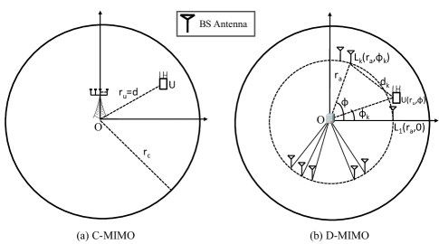
Figure 2: C-MIMO and D-MIMO systems with circular topology. Coverage areas are of circular shape with radius $r_{\mathrm{c}}$, and the antennas of D-MIMO are uniformly distributed along a circle with radius $r_{\mathrm{a}}$.

IV-B Asymptotic Spectral Efficiency in Circular Topology

Since the BS antennas are co-located in the C-MIMO scheme, the spectral efficiency is similar to (27), where $d$ is replaced by $r_{\mathrm{u}}$. In the D-MIMO setting, however, the asymptotic spectral efficiency is derived by exploiting the law of cosines, and the ensuing results are summarized in the following theorem.

Theorem 3.

For a UE located at distance $r_{\mathrm{u}}$ from the cell center of the massive C-MIMO and D-MIMO systems of circular topology, as illustrated in Fig. 2, the asymptotic spectral efficiencies are given by

$$\overline{C}_{\mathrm{C,\,circ}}\xrightarrow{p.}\sum\limits_{i=1}^{N_{T}}\log_{2}\left(1+\beta_{i}\,r_{\mathrm{u}}^{-\nu}\right)$$ (31)

and

$$\overline{C}_{\mathrm{D,\,circ}}\xrightarrow{p.}\sum\limits_{i=1}^{N_{T}}\log_{2}\left[1+\beta_{i}\,\left|r_{\mathrm{u}}^{2}-r_{\mathrm{a}}^{2}\right|^{\frac{\nu}{2}}P_{\frac{\nu}{2}-1}\left(\frac{r_{\mathrm{u}}^{2}+r_{\mathrm{a}}^{2}}{\left|r_{\mathrm{u}}^{2}-r_{\mathrm{a}}^{2}\right|}\right)\right],$$ (32)

respectively, where $\beta_{i}\triangleq N_{R}A_{i}$ and $P_{c}(x)$ refers to the Legendre function of the first kind [31, Eq. (8.820)].

Proof:

Equation (31) is immediately available by replacing $d$ in (27) with $r_{u}$. On the other hand, the proof of (32) is provided in Appendix C. ∎

From (31) and (32), similar insights to those presented after Theorem 2 can be gained. Also, by following similar procedure as in Section III-C, similar results to those in Section III-C can be obtained. More importantly, (31) and (32) can be numerically computed and serve as performance benchmark in various propagation environments. In the next subsection, we consider a typical urban environment and random values of $r_{\mathrm{u}}$, and derive asymptotic expression of the average spectral efficiency (w.r.t. $N_{R}$) for a typical user in the cell, which reflects the achievable data rate over a normalized spectral bandwidth.

IV-C Average Asymptotic Spectral Efficiency in Urban Area

Assuming transmission in an urban area with path-loss exponent $\nu=4$, for a randomly deployed UE, i.e., the value of $r_{\mathrm{u}}$ is random, we derive the average asymptotic spectral efficiency of such a typical user in the cell, in both centralized and distributed settings. We assume that $r_{\mathrm{u}}$ is uniformly distributed in $(0,r_{\mathrm{c}}]$. Then, the PDF of $r_{\mathrm{u}}$ is given by

$$f_{r_{\mathrm{u}}}(x)=\left\{\begin{array}[]{l l}\frac{2}{r_{\mathrm{c}}^{2}}x,&\quad\text{if $0<x\leq r_{\mathrm{c}}$;}\\ 0,&\quad\text{otherwise}.\end{array}\right.$$ (33)

In case of $\nu=4$, the asymptotic behaviors of C-MIMO shown in (31) and that of D-MIMO given by (32), reduce to

$$\overline{C}_{\mathrm{C,\,circ}}\xrightarrow{p.}\sum\limits_{i=1}^{N_{T}}\log_{2}\left(1+\frac{\beta_{i}}{r_{\mathrm{u}}^{4}}\right)$$ (34)

and

$$\overline{C}_{\mathrm{D,\,circ}}\xrightarrow{p.}\sum\limits_{i=1}^{N_{T}}\log_{2}\left[1+\beta_{i}\frac{r_{\mathrm{u}}^{2}+r_{\mathrm{a}}^{2}}{|r_{\mathrm{u}}^{2}-r_{\mathrm{a}}^{2}|^{3}}\right],$$ (35)

respectively.

From (34) and (35), it is evident that, by setting $r_{\mathrm{a}}\to 0$, (35) reduces to (34). Therefore, in the following we derive only the average asymptotic spectral efficiency in the D-MIMO setting w.r.t. $r_{u}$. That of the C-MIMO scheme can be readily attained by setting $r_{\mathrm{a}}\to 0$. The results are summarized in the following theorem.

Theorem 4.

The average asymptotic spectral efficiencies of the C-MIMO and D-MIMO systems in an urban area w.r.t. a uniformly distributed user in the coverage area, are given by

$$\overline{C}_{\mathrm{C,\,circ}}^{\mathrm{avg}}\xrightarrow{p.}2N_{T}\log_{2}\frac{e}{r_{\mathrm{c}}^{2}}+\sum\limits_{i=1}^{N_{T}}\log_{2}{\beta_{i}}$$ (36)

and

$$\overline{C}_{\mathrm{D,\,circ}}^{\mathrm{avg}} \xrightarrow{p.} 2N_{T}\log_{2}e-4N_{T}\frac{r_{\mathrm{a}}^{2}}{r_{\mathrm{c}}^{2}}\log_{2}r_{\mathrm{a}}^{2}$$ (37)

$$-3N_{T}\left(1-\frac{r_{\mathrm{a}}^{2}}{r_{\mathrm{c}}^{2}}\right)\log_{2}\left(r_{\mathrm{c}}^{2}-r_{\mathrm{a}}^{2}\right)$$

$$+N_{T}\left(1+\frac{r_{\mathrm{a}}^{2}}{r_{\mathrm{c}}^{2}}\right)\log_{2}\left(r_{\mathrm{c}}^{2}+r_{\mathrm{a}}^{2}\right)$$

$${}+\sum\limits_{i=1}^{N_{T}}\log_{2}{\beta_{i}},$$

respectively.

Proof:

The proof of (37) is provided in Appendix D. Equation (36) can be easily derived by setting $r_{\mathrm{a}}\to 0$ in (37). ∎

From (37), it is clear that the average spectral efficiency varies with the radius of antenna array, $r_{\mathrm{a}}$, given that the coverage radius $r_{\mathrm{c}}$ is fixed. Therefore, in the next subsection, we derive the optimal value of $r_{\mathrm{a}}$ that maximizes the average spectral efficiency given by (37).

IV-D Optimal Location of the Antenna Array in the D-MIMO Setting

After some lengthy yet straightforward algebraic manipulations, the optimal value of $r_{a}$ that maximizes the average spectral efficiency is discovered and formalized as follows.

Corollary 2.

For a massive D-MIMO system operating in an urban area, with cell radius $r_{\mathrm{c}}$, the optimal value of the radius of the circular antenna array that maximizes the average spectral efficiency given by (37) is determined by

$$r_{\mathrm{a}}^{\mathrm{opt}}=r_{\mathrm{c}}/1.31.$$ (38)

Proof:

See Appendix E. ∎

It is very interesting to see from (38) that the optimal value of the antenna array size which maximizes the average spectral efficiency given by (37), is independent of $\beta_{i}$ or $\lambda_{T,i}$, for all $i\in\{1,2,\ldots,N_{T}\}$. Thus, the optimal antenna radius in the D-MIMO setting depends neither upon the shadowing parameters nor the correlation factors, even if the shadowing and antenna correlation have severe effects on the performance of massive MIMO systems. Moreover, (38) implies that the optimal value of the antenna array size is independent of the average SNR and of the numbers of Tx/Rx antennas. These findings shed new light on the design and deployment of massive D-MIMO systems in practice.

V Numerical Results and Discussions

In this section, we present and discuss ensuing simulations results, compared with numerical ones pertaining to the analysis developed previously. The simulation experiments, of Monte Carlo type, are performed in the platform Matlab R2014a. In the simulation setting, the variance of AWGN at UE ($N_{0}$) is set to unity and, unless otherwise stated, the mean local power of the shadowing effect ($\Omega$) is normalized w.r.t. $N_{0}$ and set to $\Omega=0$ dB. Apart from Fig. 4, the sub-array spacing is set to $L_{T}=0.25{\Delta_{T}}$ and $L_{R}=0.75{\Delta_{R}}$. The spectral efficiency is in the unit of bit/s/Hz and the average SNR is in the unit of dB w.r.t. $N_{0}$. Regarding the number of Rx antennas at the BS, $N_{R}$, although no standard value has yet been specified for practical massive MIMO deployments, in densely populated areas such as stadiums where a BS may serve thousands of UEs, one can imagine that $N_{R}$ may be equal to, or even greater than, $100$ or $200$, whereas for areas with few UEs, $N_{R}$ may take smaller values such as $20$. Below, in different simulation scenarios, the value of $N_{R}$ ranges between $20$ and $200$. In Figs. 6-8 where circular topology is adopted, the radius of circular coverage area is set to $r_{\mathrm{c}}=500$ m, which is the typical value for cellular cells in up-to-date cellular networks. Finally, in all the following simulation scenarios, distance parameters are normalized w.r.t. a reference $R_{0}=500$ m. Such normalization is widely adopted in the related literature, see e.g., [30].

In the following, we first discuss the results pertaining to the asymptotic spectral efficiency for both centralized and distributed schemes, developed in Section III.

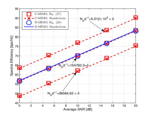
Figure 3: The asymptotic spectral efficiency of C-MIMO and D-MIMO ($\nu=3.7$, $\delta=154760.3$, $N_{R}=100$ and $N_{T}=4$).

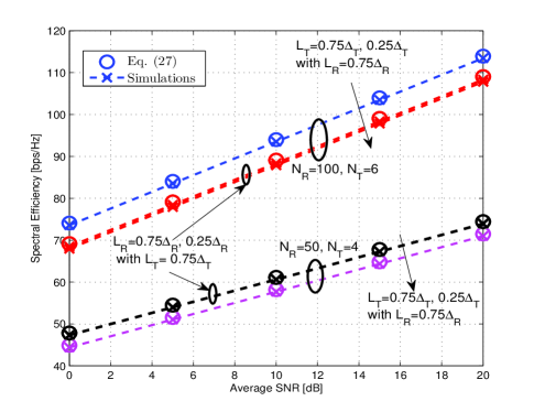
Figure 4: The asymptotic spectral efficiency of C-MIMO w.r.t. the antenna spacing ($d=0.2$ and $\nu=3.7$).

V-A Spectral-Efficiency Comparison Between C-MIMO and D-MIMO Schemes

Figure 3 compares the spectral efficiency of massive C-MIMO and D-MIMO systems. By recalling that $\delta\triangleq\sum_{k=1}^{N_{R}}d_{k}^{-\nu}$ as defined after (28) and by using the normalization w.r.t. $R_{0}$, we set, for simulation purpose, $d_{k}=R_{0}^{-1}(k+100)$, for all $k\in\{1,2,\ldots,N_{R}\}$, $\nu=3.7$, $N_{R}=100$, $N_{T}=4$, and vary the value of $d$ shown in (27). With this setting, it is easy to get $\delta=154760.3$. It is observed from the curves in the middle of Fig. 3 that $\overline{C}_{\mathrm{C}}=\overline{C}_{\mathrm{D}}$ in case of $\delta=N_{R}d^{-\nu}$. The lower curves of Fig. 3 show that $\overline{C}_{\mathrm{C}}<\overline{C}_{\mathrm{D}}$ in case of $N_{R}d^{-\nu}<\delta$, whereas the upper curves illustrate that $\overline{C}_{\mathrm{C}}>\overline{C}_{\mathrm{D}}$ in case of $N_{R}d^{-\nu}>\delta$. These observations corroborate the results obtained in Section III-B.

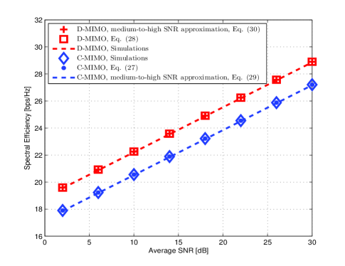
Figure 5: The asymptotic spectral efficiency of C-MIMO and D-MIMO w.r.t. the medium-to-high SNR ($d_{k}=R_{0}^{-1}(k+100)$, for all $k\in\{1,2,\ldots,N_{R}\}$, $d=0.1$, $N_{T}=1$, $N_{R}=200$ and $\nu=3.7$).

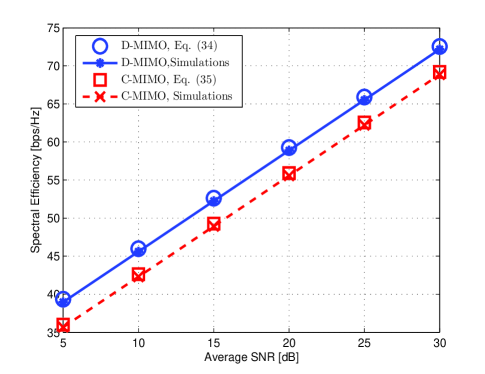
Figure 6: The asymptotic spectral efficiency of C-MIMO and D-MIMO with circular topology ($r_{\mathrm{a}}=0.2$, $r_{\mathrm{u}}=0.5$, $\nu=3.7$, $N_{T}=4$ and $N_{R}=100$).

V-B Impact of Correlation on the Asymptotic Spectral Efficiency

By recalling that in the D-MIMO scheme there is no correlation among antennas at the BS side, it is disclosed in Section III-B that the system performance of massive MIMO in both centralized and distributed settings is determined by the correlation at the UE side, in case the Weichselberger correlation model is applied. This is corroborated by observations from Fig. 4 where, for sake of clarity, only the curves related to C-MIMO are plotted. Clearly, Fig. 4 shows that by decreasing the spacing between antennas (then increasing correlation impact) at the UE side (the transmitter), the spectral efficiency of massive MIMO decreases significantly. However, changing the spacing between antennas at the BS side (the receiver), does not essentially affect the system performance. This result corroborates the previous analysis.

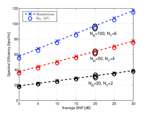
Figure 7: The average asymptotic spectral efficiency of D-MIMO with circular topology ($\nu=4$, $r_{\mathrm{a}}=0.5$).

V-C Special Case: Analysis w.r.t. Medium-to-High SNR

Figure 5 illustrates the asymptotic spectral efficiency of both massive C-MIMO and D-MIMO schemes in terms of medium-to-high SNR, as developed in Section III-C. It is observed that the approximate asymptotic behavior works perfectly for both antenna settings.

V-D A Case Study: Asymptotic Spectral Efficiency for Circularly Topology

Figure 6 presents the asymptotic spectral efficiency of massive C-MIMO and D-MIMO systems of circular topology. The cell size $r_{\mathrm{c}}$ is normalized to unity, i.e., $r_{\mathrm{c}}=1$, $r_{\mathrm{a}}=0.2$ and $r_{\mathrm{u}}=0.5$ are used in the simulation setting. It is observed from Fig. 6 that the simulation results agree perfectly with the numerical results computed as per (31) and (32), respectively.

Figure 7 shows the average asymptotic spectral efficiency for a user in a cell under the D-MIMO (by recalling that the C-MIMO scheme here is just a particular case of the D-MIMO by setting $r_{\mathrm{a}}\to 0$), in an urban area with $\nu=4$. The results are shown w.r.t. different numbers of Tx/Rx antennas, with $r_{\mathrm{a}}=0.5$. It is seen that the simulation results agree well with the numerical ones computed as per (37).

Figure 8 plots the average asymptotic spectral efficiency of massive D-MIMO being circular topology w.r.t. the normalized antenna radius, and illustrates the value of the antenna radius which maximizes the average spectral efficiency of the system. It is observed that, for different values of SNR, the maximum value of the average spectral efficiency always appears at $r_{\mathrm{a}}\approx 0.76$, which is consistent with our analytical result given by (38), i.e., $r_{\mathrm{a}}^{\mathrm{opt}}=r_{\mathrm{c}}/1.31\approx 0.76$.

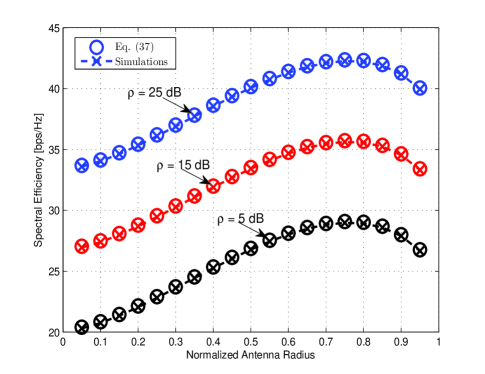
Figure 8: Optimal value of the antenna array size that maximizes the average spectral efficiency of D-MIMO ($\nu=4$).

VI Concluding Remarks

In this paper, the spectral efficiency of massive MIMO systems in both centralized (C-MIMO) and distributed (D-MIMO) settings, was analytically investigated, based on a novel comprehensive analytical channel model where major natural environmental and antenna physical parameters were accounted for, including path loss, shadowing, multi-path fading and antenna correlation. Our results reveal that the C-MIMO scheme does not always underperform D-MIMO, although the latter exhibits a higher multiplexing gain. Further, the uplink performance of massive MIMO is shown to be mainly determined by the antenna correlation at the UE side, given that the Weichselberger correlation model is applied. For practical purposes, it was demonstrated that for the D-MIMO scheme with circular topology of radius $r_{\mathrm{c}}$, the optimal value of the radius of antenna array that maximizes the average spectral efficiency is given by $r_{\mathrm{a}}^{\mathrm{opt}}=r_{\mathrm{c}}/1.31$. The proposed channel model, the developed analysis and the obtained results, thanks to their generality and compactness, can serve as practical benchmark for designing and analyzing performances of massive MIMO systems in real physical propagation environments.

Appendix A Proof of Lemma 1

With the vectors $\mathbf{p}$ and $\mathbf{q}$ defined in Lemma 1, we have $\mathbf{p}^{\rm H}\mathbf{p}=\sum_{k=1}^{n}a_{k}|p_{k}|^{2}$ and $\mathbb{E}\left\{\mathbf{p}^{\rm H}\mathbf{p}\right\}=\sum_{k=1}^{n}a_{k}\mu_{p,k}$. Let $z$ be a constant which satisfies (23). It is then clear that $\mathrm{Var}\left\{|a_{i}^{\frac{1}{2}}p_{i}|^{2}\right\}=|a_{i}|^{2}\sigma^{2}_{p,i}<\infty$. Therefore, by applying the well-known law of large numbers for i.n.i.d. RVs [32, p. 313] to $a_{i}^{\frac{1}{2}}p_{i}$, the entries of $\mathbf{p}$, (24) is easily attained.

On the other hand, since $p_{i}$ and $q_{i}$ are independent, we have $\mathbb{E}\left\{p_{i}^{\rm H}q_{i}\right\}=0$, for all $i\in\left\{1,2,\cdots,n\right\}$. Finally, by following similar steps as in the proof of (24), (25) can be readily proven.

$$\mathbf{M}_{\mathrm{J}}=\begin{bmatrix}\sum\limits_{k=1}^{N_{R}}\lambda_{T,1}\lambda_{R,k}d_{k}^{-\nu}{\varphi}_{k}|\widehat{H}_{k,1}|^{2}&\sum\limits_{k=1}^{N_{R}}\lambda_{T,1}^{\frac{1}{2}}\lambda_{T,2}^{\frac{1}{2}}\lambda_{R,k}d_{k}^{-\nu}{\varphi}_{k}\widehat{H}_{k,1}^{\rm H}{\widehat{H}_{k,2}}&\cdots&\sum\limits_{k=1}^{N_{R}}\lambda_{T,1}^{\frac{1}{2}}\lambda_{T,N_{T}}^{\frac{1}{2}}\lambda_{R,k}d_{k}^{-\nu}{\varphi}_{k}{\widehat{H}_{k,1}}^{\rm H}\widehat{H}_{k,N_{T}}\\ \sum\limits_{k=1}^{N_{R}}\lambda_{T,2}^{\frac{1}{2}}\lambda_{T,1}^{\frac{1}{2}}\lambda_{R,k}d_{k}^{-\nu}{\varphi}_{k}{\widehat{H}_{k,2}}^{\rm H}\widehat{H}_{k,1}&\sum\limits_{k=1}^{N_{R}}\lambda_{T,2}\lambda_{R,k}d_{k}^{-\nu}{\varphi}_{k}|\widehat{H}_{k,2}|^{2}&\cdots&\sum\limits_{k=1}^{N_{R}}\lambda_{T,2}^{\frac{1}{2}}\lambda_{T,N_{T}}^{\frac{1}{2}}\lambda_{R,k}d_{k}^{-\nu}{\varphi}_{k}{\widehat{H}_{k,2}}^{\rm H}\widehat{H}_{k,N_{T}}\\ \vdots&\vdots&\ddots&\vdots\\ \sum\limits_{k=1}^{N_{R}}\lambda_{T,N_{T}}^{\frac{1}{2}}\lambda_{T,1}^{\frac{1}{2}}\lambda_{R,k}d_{k}^{-\nu}{\varphi}_{k}{\widehat{H}_{k,N_{T}}}^{\rm H}\widehat{H}_{k,1}&\sum\limits_{k=1}^{N_{R}}\lambda_{T,N_{T}}^{\frac{1}{2}}\lambda_{T,2}^{\frac{1}{2}}\lambda_{R,k}d_{k}^{-\nu}{\varphi}_{k}{\widehat{H}_{k,N_{T}}}^{\rm H}\widehat{H}_{k,2}&\cdots&\sum\limits_{k=1}^{N_{R}}\lambda_{T,N_{T}}\lambda_{R,k}d_{k}^{-\nu}{\varphi}_{k}|\widehat{H}_{k,N_{T}}|^{2}\end{bmatrix}.$$ (40)

$$\frac{1}{N_{R}}\mathbf{g}_{i}^{\rm H}\mathbf{h}_{j}\xrightarrow{p.}\frac{1}{N_{R}}\mathbb{E}\{[\mathbf{M}_{\mathrm{J}}]_{i,j}\}\overset{p.}{\longrightarrow} 0, i\neq j$$ ; (45)

$$\frac{1}{N_{R}}\mathbf{g}_{i}^{\rm H}\mathbf{h}_{j}\xrightarrow{p.}\frac{1}{N_{R}}\mathbb{E}\{[\mathbf{M}_{\mathrm{J}}]_{i,j}\}\overset{p.}{\longrightarrow} \frac{1}{N_{R}}\sum\limits_{k=1}^{N_{R}}\lambda_{T,i}\,d_{k}^{-\nu}\Omega, i=j$$ . (46)

$$\mathbf{M}_{\mathrm{J}}=N_{R}\left(\frac{1}{N_{R}}\mathbf{M}_{\mathrm{D}}\right)\overset{p.}{\longrightarrow}\mathrm{diag}\left\{\sum\limits_{k=1}^{N_{R}}d_{k}^{-\nu}\lambda_{T,1}\Omega,\sum\limits_{k=1}^{N_{R}}d_{k}^{-\nu}\lambda_{T,2}\Omega,\ldots,\sum\limits_{k=1}^{N_{R}}d_{k}^{-\nu}\lambda_{T,N_{T}}\Omega\right\}.$$ (47)

Appendix B Proof of Theorem 1

We first derive the explicit expressions of matrices $\mathbf{G}_{\mathrm{C}}$ and $\mathbf{G}_{\mathrm{D}}$ uniformly defined in (13). By substituting (14) and (15) into (13) and recalling that $\lambda_{R,k}=1$, for all $k\in\{1,2,\ldots,N_{R}\}$, if $\mathrm{J}=\mathrm{D}$ (as $\mathbf{\Theta}_{R}$ reduces to $\mathbf{I}_{N_{R}}$ in the D-MIMO setting), $\mathbf{G}_{\mathrm{C}}$ and $\mathbf{G}_{\mathrm{D}}$ can be uniformly expressed as

$$\mathbf{G}_{\mathrm{J}}=\begin{bmatrix}\lambda_{R,1}^{\frac{1}{2}}\lambda_{T,1}^{\frac{1}{2}}&\lambda_{R,1}^{\frac{1}{2}}\lambda_{T,2}^{\frac{1}{2}}&\cdots&\lambda_{R,1}^{\frac{1}{2}}\lambda_{T,N_{T}}^{\frac{1}{2}}\\ \lambda_{R,2}^{\frac{1}{2}}\lambda_{T,1}^{\frac{1}{2}}&\lambda_{R,2}^{\frac{1}{2}}\lambda_{T,2}^{\frac{1}{2}}&\cdots&\lambda_{R,2}^{\frac{1}{2}}\lambda_{T,N_{T}}^{\frac{1}{2}}\\ \vdots&\vdots&\ddots&\vdots\\ \lambda_{R,N_{R}}^{\frac{1}{2}}\lambda_{T,1}^{\frac{1}{2}}&\lambda_{R,N_{R}}^{\frac{1}{2}}\lambda_{T,2}^{\frac{1}{2}}&\cdots&\lambda_{R,N_{R}}^{\frac{1}{2}}\lambda_{T,N_{T}}^{\frac{1}{2}}\end{bmatrix},~{}\forall\mathrm{J}\in\{\mathrm{C},\mathrm{D}\},$$ (39)

where $\lambda_{R,k}\equiv 1$, for all $k\in\{1,2,\ldots,N_{R}\}$, if $\mathrm{J}=\mathrm{D}$. Then, substituting (39) into the expression of $\mathbf{M}_{\mathrm{C}}$ given by (19) if $\mathrm{J}=\mathrm{C}$, or (39) into the expression of $\mathbf{M}_{\mathrm{D}}$ shown in (20) if $\mathrm{J}=\mathrm{D}$, and after performing some algebraic manipulations, we attain (40) shown at the top of this page, where $\widehat{H}_{i,j}$ denotes the $(i,j)^{\mathrm{th}}$ entry of $\mathbf{\widehat{H}}$ shown in (6), and where $d_{k}=d$ and ${\varphi}_{k}={\varphi}$ if $\mathrm{J}=\mathrm{C}$ whereas $\lambda_{R,k}=1$ if $\mathrm{J}=\mathrm{D}$, for all $k\in\{1,2,\ldots,N_{R}\}$.

In view of (40), it is clear that the $(i,j)^{\mathrm{th}}$ entry, for all $i,j\in\{1,2,\ldots,N_{T}\}$, of $\mathbf{M}_{\mathrm{C}}$ and $\mathbf{M}_{\mathrm{D}}$, are given by

$$[\mathbf{M}_{\mathrm{J}}]_{i,j}=\sum\limits_{k=1}^{N_{R}}\lambda_{T,i}^{\frac{1}{2}}\lambda_{T,j}^{\frac{1}{2}}\lambda_{R,k}d_{k}^{-\nu}{\varphi}_{k}{\widehat{H}_{k,i}}^{\rm H}\widehat{H}_{k,j},~{}\forall\mathrm{J}\in\{\mathrm{C},\mathrm{D}\},$$ (41)

where $d_{k}\equiv d$ and ${\varphi}_{k}\equiv{\varphi}$ if $\mathrm{J}=\mathrm{C}$ whereas $\lambda_{R,k}=1$ if $\mathrm{J}=\mathrm{D}$, for all $k\in\{1,2,\ldots,N_{R}\}$.

In order to apply Lemma 1, we need check the condition shown in (23). Specifically, for all $i,j\in\{1,2,\ldots,N_{T}\}$, let

$$\mathbf{g}_{i}\triangleq\left[a_{1,i}^{\frac{1}{2}}{g}_{1,i},a_{2,i}^{\frac{1}{2}}{g}_{2,i},\cdots,a_{N_{R},i}^{\frac{1}{2}}{g}_{N_{R},i}\right]^{\rm T}$$ (42)

and

$$\mathbf{h}_{j}\triangleq\left[b_{1,j}^{\frac{1}{2}}{h}_{1,j},b_{2,j}^{\frac{1}{2}}{h}_{2,j},\cdots,b_{N_{R},j}^{\frac{1}{2}}{h}_{N_{R},j}\right]^{\rm T},$$ (43)

where in the C-MIMO setting, $a_{k,i}\triangleq\lambda_{T,i}\lambda_{R,k}d^{-\nu}$, $b_{k,j}\triangleq\lambda_{T,j}\lambda_{R,k}d^{-\nu}$, ${g}_{k,i}\triangleq{\varphi}^{\frac{1}{2}}\widehat{H}_{k,i}$ and ${h}_{k,j}\triangleq{\varphi}^{\frac{1}{2}}\widehat{H}_{k,j}$, for all $k\in\{1,2,\ldots,N_{R}\}$, whereas in the D-MIMO setting, $a_{k,i}\triangleq\lambda_{T,i}d_{k}^{-\nu}$, $b_{k,j}\triangleq\lambda_{T,j}d_{k}^{-\nu}$, ${g}_{k,i}\triangleq{\varphi}_{k}^{\frac{1}{2}}{\widehat{H}_{k,i}}$ and ${h}_{k,j}\triangleq{\varphi}_{k}^{\frac{1}{2}}\widehat{H}_{k,j}$, for all $k\in\{1,2,\ldots,N_{R}\}$. With these definitions in mind, it is clear that $[\mathbf{M}_{\mathrm{C}}]_{i,j}$ shown in (41) equals $\mathbf{g}_{i}^{\rm H}\mathbf{h}_{j}$ where $\mathbf{g}_{i}$ and $\mathbf{h}_{j}$ are expressed as in the C-MIMO setting, and that $[\mathbf{M}_{\mathrm{D}}]_{i,j}$ shown in (41) equals $\mathbf{g}_{i}^{\rm H}\mathbf{h}_{j}$ where $\mathbf{g}_{i}$ and $\mathbf{h}_{j}$ are expressed as in the D-MIMO setting. The correlation matrices $\mathbf{\Theta}_{T}$ and $\mathbf{\Theta}_{R}$ shown in (10) are of Toeplitz form [33]. Also, it is well-known that for large numbers of antennas, the eigenvalues of $\mathbf{\Theta}$ ($\mathbf{\Theta}_{T}$ or $\mathbf{\Theta}_{R}$) converge uniformly to [33, p. 38]

$$\lambda_{\mathbf{\Theta}}(x)=(1-\theta^{2})(1-2\,\theta\cos(2\pi x)+\theta^{2})^{-1},$$ (44)

where $\theta={\theta}_{T}$ (resp. $\theta={\theta}_{R}$) for $\mathbf{\Theta}=\mathbf{\Theta}_{T}$ (resp. $\mathbf{\Theta}=\mathbf{\Theta}_{R}$), with $\theta_{T}$ and $\theta_{R}$ defined immediately after (10), and where $x\in\left[0,1\right]$. According to (44), the maximum eigenvalue of $\mathbf{\Theta}$ in the massive MIMO context is then obtained by setting $x=0$ in the denominator of (44), yielding $\lambda_{\mathbf{\Theta},\,\mathrm{max}}=(1+\theta)(1-\theta)^{-1}$, which is a finite real number, and, therefore, it is clear that there exists $b<\infty$ such that $a_{k,i}^{2}\leq b$ and $b_{k,j}^{2}\leq b$, for all $i,j\in\{1,2,\ldots,N_{T}\}$ and, hence, the condition required by Lemma 1 is satisfied.

Now, recalling that for all $i,j\in\{1,2,\ldots,N_{T}\}$ and for all $k\in\{1,2,\ldots,N_{R}\}$, $\widehat{H}_{k,i},\widehat{H}_{k,j}\sim\mathcal{CN}(0,1)$ according to (7), it is clear that $\mathbb{E}\{[\mathbf{M}_{\mathrm{C}}]_{i,j}\}=\mathbb{E}\{[\mathbf{M}_{\mathrm{D}}]_{i,j}\}=0$, for all $i\neq j$. On the other hand, if $i=j$, by recalling the Gamma distribution of ${\varphi}$ and ${\varphi}_{k}$, $k\in\{1,2,\ldots,N_{R}\}$, as shown respectively in (4) and (5), and recalling that $\widehat{H}_{i,j}\sim\mathcal{CN}(0,1)$ as shown in (7), and with further algebraic manipulations, the mean of the diagonal entries of $\mathbf{M}_{\mathrm{C}}$ and $\mathbf{M}_{\mathrm{D}}$ are obtained as $\mathbb{E}\{[\mathbf{M}_{\mathrm{C}}]_{i,i}\}=N_{R}\lambda_{T,i}\,d^{-\nu}\Omega$ and $\mathbb{E}\{[\mathbf{M}_{\mathrm{D}}]_{i,i}\}=\lambda_{T,i}\sum_{k=1}^{N_{R}}d_{k}^{-\nu}\Omega$, respectively.

Finally, by recalling that the entries of $\mathbf{g}_{i}$ and $\mathbf{h}_{j}$ shown respectively in (42) and (43) depend upon the scheme (C-MIMO or D-MIMO) as presented right after (43), and noticing that $\mathbf{g}_{i}=\mathbf{h}_{j}$ if $i=j$ within each of the schemes, and assuming $N_{R}\to\infty$, we apply Lemma 1 to the vectors $\mathbf{g}_{i}$ and $\mathbf{h}_{j}$, yielding (45) and (46) shown at the top of this page, where $d_{k}\equiv d$, for all $k\in\{1,2,\ldots,N_{R}\}$, if $\mathrm{J}=\mathrm{C}$. By virtue of (45) and (46), we attain (47), shown also at the top of this page, where $d_{k}\equiv d$, for all $k\in\{1,2,\ldots,N_{R}\}$, if $\mathrm{J}=\mathrm{C}$. This completes the proof.

Appendix C Proof of Eq. (32)

In view of Fig. 2-b and by recalling the well-known law of cosines in geometry, we have, for all $k\in\{1,2,\ldots,N_{R}\}$, $d_{k}=\left[r_{\mathrm{u}}^{2}+r_{\mathrm{a}}^{2}-2r_{\mathrm{u}}r_{\mathrm{a}}\cos(\phi_{k}-\phi)\right]^{1/2}=\left(r_{\mathrm{u}}^{2}+r_{\mathrm{a}}^{2}-2r_{\mathrm{u}}r_{\mathrm{a}}\cos\omega_{k}\right)^{1/2}$, where $\omega_{k}\triangleq\phi_{k}-\phi$ is the angle between the segments $OU$ and $OL_{k}$. Let $\Delta\omega\triangleq\omega_{k+1}-\omega_{k}$. Then, by recalling that $\phi_{1}=0$ and that $\phi_{k}=2\pi(k-1)/{N_{R}}$, for all $k\in[2,N_{R}]$ (cf. Section IV-A), we have $\Delta\omega=2\pi/{N_{R}}$. Therefore, if $N_{R}\to\infty$, we have

$$\frac{1}{N_{R}}\sum\limits_{k=1}^{N_{R}}d_{k}^{-\nu} =\frac{1}{N_{R}\,\Delta\omega}\sum\limits_{k=1}^{N_{R}}\left(r_{\mathrm{u}}^{2}+r_{\mathrm{a}}^{2}-2r_{\mathrm{u}}r_{\mathrm{a}}\cos\omega_{k}\right)^{-\nu/2}\Delta\omega$$ (48)

$$\xrightarrow{N_{R}\to\infty}\frac{1}{2\pi}\int_{0}^{2\pi}\left(r_{\mathrm{u}}^{2}+r_{\mathrm{a}}^{2}-2r_{\mathrm{u}}r_{\mathrm{a}}\cos\omega\right)^{-\nu/2}\mathrm{d}\omega$$ (49)

$$=\frac{1}{2\pi}\int_{-\pi}^{\pi}\left(r_{\mathrm{u}}^{2}+r_{\mathrm{a}}^{2}-2r_{\mathrm{u}}r_{\mathrm{a}}\cos\omega\right)^{-\nu/2}\mathrm{d}\omega,$$ (50)

where the identity $\int_{0}^{2\pi}\cos\omega\,\mathrm{d}\omega=\int_{-\pi}^{\pi}\cos\omega\,\mathrm{d}\omega$ was exploited to derive (50). Finally, applying [34, Eq. (2.5.16.38)] to (50) and performing some algebraic manipulations yields (32).

Appendix D Proof of Theorem 4

In the D-MIMO scheme, to obtain simple yet meaningful expression of the average asymptotic spectral efficiency of the system, we consider the range of medium-to-high SNR, where $\beta_{i}=\rho\Omega N_{R}\lambda_{T,i}N_{T}^{-1}\overset{N_{R}\to\infty}{\longrightarrow}\infty$, for all $i\in\{1,2,\ldots,N_{T}\}$. The average asymptotic spectral efficiency of the system in this case is then derived as

$$\overline{C}_{\mathrm{D,\,circ}}^{\mathrm{avg}} =\int_{0}^{r_{\mathrm{c}}}f_{r_{\mathrm{u}}}(x)\overline{C}_{\mathrm{D,\,circ}}(r_{\mathrm{u}})\,\mathrm{d}{r_{\mathrm{u}}}$$ (51)

$$\xrightarrow{p.}\frac{2}{r_{\mathrm{c}}^{2}\ln 2}\sum\limits_{i=1}^{N_{T}}\int_{0}^{r_{\mathrm{c}}}r_{\mathrm{u}}\ln\left[1+\beta_{i}\frac{r_{\mathrm{u}}^{2}+r_{\mathrm{a}}^{2}}{|r_{\mathrm{u}}^{2}-r_{\mathrm{a}}^{2}|^{3}}\right]\,\mathrm{d}{r_{\mathrm{u}}}$$ (52)

$$\approx\frac{1}{r_{\mathrm{c}}^{2}\ln 2}\sum\limits_{i=1}^{N_{T}}\int_{0}^{r_{\mathrm{c}}^{2}}\ln\left[\beta_{i}\frac{y+r_{\mathrm{a}}^{2}}{|y-r_{\mathrm{a}}^{2}|^{3}}\right]\,\mathrm{d}y$$ (53)

$$=\frac{1}{r_{\mathrm{c}}^{2}\ln 2}\!\sum\limits_{i=1}^{N_{T}}\!\left\{\!\int_{0}^{r_{\mathrm{c}}^{2}}\!\!\!\ln\beta_{i}\,\mathrm{d}y\!+\!\!\int_{0}^{r_{\mathrm{c}}^{2}}\!\!\!\ln(y+r_{a}^{2})\,\mathrm{d}y\right.$$

$$\quad\left.-3\!\!\int_{0}^{r_{\mathrm{a}}^{2}}\!\!\!\ln(r_{a}^{2}-y)\,\mathrm{d}y-3\!\!\int_{r_{\mathrm{a}}^{2}}^{r_{\mathrm{c}}^{2}}\!\!\!\!\ln(y-r_{a}^{2})\,\mathrm{d}y\right\},$$ (54)

where the approximation $\ln(1+x)\approx\ln x$ if $x\to\infty$ was used along with the change of variable $y=r_{\mathrm{a}}^{2}$, to obtain (53). Finally, solving the integrals involved in (54) and performing further algebraic manipulations, leads to the intended (37).

Appendix E Proof of Corollary 2

The first-order derivative of the average asymptotic spectral efficiency, i.e., $\overline{C}_{\mathrm{D,\,circ}}^{\mathrm{avg}}$ given by (37), w.r.t. the antenna array size $r_{\mathrm{a}}$, is given by

$$\frac{\mathrm{d}}{\mathrm{d}r_{\mathrm{a}}}\overline{C}_{\mathrm{D,\,circ}}^{\mathrm{avg}}=6N_{T}\frac{r_{\mathrm{a}}}{r_{\mathrm{c}}^{2}}\log_{2}(\chi-2)+2N_{T}\frac{r_{\mathrm{a}}}{r_{\mathrm{c}}^{2}}\log_{2}\chi,$$ (55)

where $\chi\triangleq r_{\mathrm{c}}^{2}/r_{\mathrm{a}}^{2}+1$. Then, by setting $\frac{\mathrm{d}}{\mathrm{d}r_{\mathrm{a}}}\overline{C}_{\mathrm{D,\,circ}}^{\mathrm{avg}}=0$ and performing some algebraic manipulations, we get the equation $(r_{\mathrm{c}}^{2}-r_{\mathrm{a}}^{2})^{3}(r_{\mathrm{c}}^{2}+r_{\mathrm{a}}^{2})-r_{\mathrm{a}}^{8}=0$, which can be reformulated as

$$\chi(\chi-2)^{3}-1=0\,\,\iff\,\,\chi^{\frac{4}{3}}-2\chi^{\frac{1}{3}}-1=0.$$ (56)

After performing some algebraic manipulations, the solution to (56), denoted $\chi_{0}$, can be readily shown as $\chi_{0}=2.7167$. Finally, by using the definition of $\chi$ right after (55), we attain (38).

On the other hand, by multiplying both sides of (55) by $1/r_{\mathrm{a}}$, it is clear that the function $\frac{1}{r_{\mathrm{a}}}\frac{\mathrm{d}}{\mathrm{d}r_{\mathrm{a}}}\overline{C}_{\mathrm{D,\,circ}}^{\mathrm{avg}}$ is decreasing with $r_{\mathrm{a}}$, then $\frac{1}{r_{\mathrm{a}}}\frac{\mathrm{d}}{\mathrm{d}r_{\mathrm{a}}}\overline{C}_{\mathrm{D,\,circ}}^{\mathrm{avg}}<0$ if $r_{\mathrm{a}}<r_{\mathrm{a}}^{\mathrm{opt}}$, and $\frac{1}{r_{\mathrm{a}}}\frac{\mathrm{d}}{\mathrm{d}r_{\mathrm{a}}}\overline{C}_{\mathrm{D,\,circ}}^{\mathrm{avg}}>0$ if $r_{\mathrm{a}}>r_{\mathrm{a}}^{\mathrm{opt}}$. Since $r_{\mathrm{a}}>0$, we have $\frac{\mathrm{d}}{\mathrm{d}r_{\mathrm{a}}}\overline{C}_{\mathrm{D,\,circ}}^{\mathrm{avg}}<0$ if $r_{\mathrm{a}}<r_{\mathrm{a}}^{\mathrm{opt}}$, and $\frac{\mathrm{d}}{\mathrm{d}r_{\mathrm{a}}}\overline{C}_{\mathrm{D,\,circ}}^{\mathrm{avg}}>0$ if $r_{\mathrm{a}}>r_{\mathrm{a}}^{\mathrm{opt}}$, which concludes that $r_{\mathrm{a}}^{\mathrm{opt}}$ is the maximum of the average asymptotic spectral efficiency.

Gervais N. Kamga (S’13) received the B.S. degree in Electrical and Computer Engineering from Ecole Mohammadia d’Ingénieurs (EMI), Rabat, Morocco, in 2011. He joined the Institut National de la Recherche Scientifique (INRS), University of Quebec, Montreal, QC, Canada, where he is currently working towards the Ph.D. degree in Telecommunications. Gervais was a prize winner of the Pan African Mathematics Olympiads in 2006. He was a recipient of the Excellence Scholarship for International Cooperation Morocco-Cameroon, and the Financial Assistance of the State of Cameroon to Scholarship Students Abroad, from 2006 to 2011. Between 2010 and 2011, he won, respectively, the National Students Open Design and Innovation Competition (SODEC), and the National Competition for Technological Innovation (EMINOV), Morocco. He was also a finalist in the 2010 EMINOV. In 2011, he was a recipient of the International ParisTech and Renault Foundation scholarship for the Mobility and Electric Vehicles Master s Program. At INRS, he is recipient of a waiver of high tuition fees for foreign students, and university scholarship for graduate studies. He was, in 2013, a semi-finalist to the Quebec National Concours Forces Avenir, in the Sciences and Technology Applications category.

Minghua Xia (M’12) obtained his Ph.D. degree in Telecommunications and Information Systems from Sun Yat-sen University, Guangzhou, China, in 2007. Since 2015, he has been working as a Professor at the same university. From 2007 to 2009, he was with the Electronics and Telecommunications Research Institute (ETRI) of South Korea, Beijing R&D Center, Beijing, China, where he worked as a member and then as a senior member of engineering staff and participated in the projects on the physical layer design of 3GPP LTE mobile communications. From 2010 to 2014, he was in sequence with The University of Hong Kong, Hong Kong, China; King Abdullah University of Science and Technology, Jeddah, Saudi Arabia; and the Institut National de la Recherche Scientifique (INRS), University of Quebec, Montreal, Canada, as a Postdoctoral Fellow. His research interests are in the general area of 5G wireless communications, and in particular the design and performance analysis of multi-antenna systems, cooperative relaying systems and cognitive relaying networks, and recently focus on the design and analysis of wireless power transfer and/or energy harvesting systems, as well as massive MIMO and small cells. He holds two patents granted in China. Dr. Xia received the Professional Award at IEEE TENCON’15, Macau, 2015. He was also awarded as an Exemplary Reviewer by IEEE Transactions on Communications, IEEE Communications Letters, and IEEE Wireless Communications Letters, respectively, in 2014.

Sonia Aïssa (S’93-M’00-SM’03) received her Ph.D. degree in Electrical and Computer Engineering from McGill University, Montreal, QC, Canada, in 1998. Since then, she has been with the Institut National de la Recherche Scientifique-Energy, Materials and Telecommunications Center (INRS-EMT), University of Quebec, Montreal, QC, Canada, where she is a Full Professor. From 1996 to 1997, she was a Researcher with the Department of Electronics and Communications of Kyoto University, and with the Wireless Systems Laboratories of NTT, Japan. From 1998 to 2000, she was a Research Associate at INRS-EMT. In 2000-2002, while she was an Assistant Professor, she was a Principal Investigator in the major program of personal and mobile communications of the Canadian Institute for Telecommunications Research, leading research in radio resource management for wireless networks. From 2004 to 2007, she was an Adjunct Professor with Concordia University, Montreal. She was Visiting Invited Professor at Kyoto University, Japan, in 2006, and Universiti Sains Malaysia, in 2015. Her research interests include the modeling, design and performance analysis of wireless communication systems and networks. Dr. Aïssa is the Founding Chair of the IEEE Women in Engineering Affinity Group in Montreal, 2004-2007; acted as TPC Symposium Chair or Cochair at IEEE ICC ’06 ’09 ’11 ’12; Program Cochair at IEEE WCNC 2007; TPC Cochair of IEEE VTC-spring 2013; and TPC Symposia Chair of IEEE Globecom 2014. Her main editorial activities include: Editor, IEEE Transactions on Wireless Communications, 2004-2012; Associate Editor and Technical Editor, IEEE Communications Magazine, 2004-2015; Technical Editor, IEEE Wireless Communications Magazine, 2006-2010; and Associate Editor, Wiley Security and Communication Networks Journal, 2007-2012. She currently serves as Area Editor for the IEEE Transactions on Wireless Communications. Awards to her credit include the NSERC University Faculty Award in 1999; the Quebec Government FRQNT Strategic Faculty Fellowship in 2001-2006; the INRS-EMT Performance Award multiple times since 2004, for outstanding achievements in research, teaching and service; and the Technical Community Service Award from the FQRNT Centre for Advanced Systems and Technologies in Communications, 2007. She is co-recipient of five IEEE Best Paper Awards and of the 2012 IEICE Best Paper Award; and recipient of NSERC Discovery Accelerator Supplement Award. She is a Distinguished Lecturer of the IEEE Communications Society (ComSoc) and an Elected Member of the ComSoc Board of Governors. Professor Aïssa is a Fellow of the Canadian Academy of Engineering.

References

- [1] E. Larsson, O. Edfors, F. Tufvesson, and T. Marzetta, “Massive MIMO for next generation wireless systems,” IEEE Commun. Mag., vol. 52, no. 2, pp. 186–195, Feb. 2014.
- [2] J. G. Andrews, S. Buzzi, W. Choi, S. V. Hanly, A. Lozano, A. C. K. Soong, and J. C. Zhang, “What will 5G be?” IEEE J. Select. Areas Commun., vol. 32, no. 6, pp. 1065–1082, June 2014.
- [3] E. Björnson, M. Matthaiou, and M. Debbah, “Massive MIMO with non-ideal arbitrary arrays: Hardware scaling laws and circuit-aware design,” IEEE Trans. Wireless Commun., vol. 14, no. 8, pp. 4353–4368, Aug. 2015.
- [4] S. Firouzabadi and A. Goldsmith, “Optimal placement of distributed antennas in cellular systems,” in Proc. IEEE SPAWC’11, June 2011, pp. 461–465.
- [5] D. Wang, J. Wang, X. You, Y. Wang, M. Chen, and X. Hou, “Spectral efficiency of distributed MIMO systems,” IEEE J. Select. Areas Commun., vol. 31, no. 10, pp. 2112–2127, Oct. 2013.
- [6] X. Wang, P. Zhu, and M. Chen, “Antenna location design for generalized distributed antenna systems,” IEEE Commun. Lett., vol. 13, no. 5, pp. 315–317, May 2009.
- [7] H. Xia, A. Herrera, S. Kim, and F. Rico, “A CDMA-distributed antenna system for in-building personal communications services,” IEEE J. Select. Areas Commun., vol. 14, no. 4, pp. 644–650, May 1996.
- [8] R. Schuh and M. Sommer, “W-CDMA coverage and capacity analysis for active and passive distributed antenna systems,” in Proc. IEEE VTC’02-Spring, vol. 1, 2002, pp. 434–438.
- [9] A. Chockalingam and B. S. Rajan, Large MIMO Systems. Cambridge University Press, Feb. 2014.
- [10] C.-N. Chuah, D. Tse, J. Kahn, and R. Valenzuela, “Capacity scaling in MIMO wireless systems under correlated fading,” IEEE Trans. Inf. Theory, vol. 48, no. 3, pp. 637–650, Mar. 2002.
- [11] E. Telatar, “Capacity of multi-antenna Gaussian channels,” Eur. Trans. Telecommun., vol. 10, no. 6, pp. 585–595, Sep. 1999.
- [12] A. Goldsmith, S. Jafar, N. Jindal, and S. Vishwanath, “Capacity limits of MIMO channels,” IEEE J. Select. Areas Commun., vol. 21, no. 5, pp. 684–702, June 2003.
- [13] A. Tulino, A. Lozano, and S. Verdu, “Impact of antenna correlation on the capacity of multi-antenna channels,” IEEE Trans. Inf. Theory, vol. 51, no. 7, pp. 2491–2509, July 2005.
- [14] V. V. Veeravalli, Y. Liang, and A. Sayeed, “Correlated MIMO Rayleigh fading channels: Capacity, optimal signaling, and scaling laws,” IEEE Trans. Inf. Theory, vol. 51, no. 6, pp. 2058–2072, June 2005.
- [15] V. Raghavan and A. Sayeed, “Sublinear capacity scaling laws for sparse MIMO channels,” IEEE Trans. Inf. Theory, vol. 57, no. 1, pp. 345–364, Jan. 2011.
- [16] G. N. Kamga, M. Xia, and S. Aïssa, “Channel modeling and capacity analysis of MIMO systems in real propagation environments,” IEEE Trans. Wireless Commun., submitted for possible publication.
- [17] G. Kamga, M. Xia, and S. Aïssa, “Channel modelling and capacity analysis of large MIMO in real propagation environments,” in Proc. IEEE ICC’15, June 2015, pp. 1447–1452.
- [18] C. Oestges, B. Clerckx, M. Guillaud, and M. Debbah, “Dual-polarized wireless communications: From propagation models to system performance evaluation,” IEEE Trans. Wireless Commun., vol. 7, no. 10, pp. 4019–4031, Oct. 2008.
- [19] A. Maaref and S. Aïssa, “Impact of spatial fading correlation and keyhole on the capacity of MIMO systems with transmitter and receiver CSI,” IEEE Trans. Wireless Commun., vol. 7, no. 8, pp. 3218–3229, Aug. 2008.
- [20] N. Costa and S. Haykin, Multiple-Input Multiple-Output Channel Models: Theory and Practice. John Wiley & Sons, 2010.
- [21] W. Weichselberger, M. Herdin, H. Ozcelik, and E. Bonek, “A stochastic MIMO channel model with joint correlation of both link ends,” IEEE Trans. Wireless Commun., vol. 5, no. 1, pp. 90–100, Jan. 2006.
- [22] X. Gao, M. Zhu, F. Rusek, F. Tufvesson, and O. Edfors, “Large antenna array and propagation environment interaction,” in Proc. ACSSC’14, Nov. 2014, pp. 666–670.
- [23] H. Ozcelik, M. Herdin, W. Weichselberger, J. Wallace, and E. Bonek, “Deficiencies of ‘Kronecker’ MIMO radio channel model,” Electron. Lett., vol. 39, no. 16, pp. 1209–1210, Aug. 2003.
- [24] V. Raghavan, J. H. Kotecha, and A. Sayeed, “Why does the Kronecker model result in misleading capacity estimates?” IEEE Trans. Inf. Theory, vol. 56, no. 10, pp. 4843–4864, Oct. 2010.
- [25] W. Weichselberger, “Spatial structure of multiple antenna radio channels–A signal processing viewpoint,” Ph.D. dissertation, Technische Universität Wien, Dec. 2003.
- [26] E. Björnson, E. G. Larsson, and T. L. Marzetta, “Massive MIMO: Ten myths and one critical question,” IEEE Commun. Mag., to appear. [Online]. Available: arXiv:1503.06854v2
- [27] H. Q. Ngo, E. Larsson, and T. Marzetta, “Energy and spectral efficiency of very large multiuser MIMO systems,” IEEE Trans. Commun., vol. 61, no. 4, pp. 1436–1449, April 2013.
- [28] A. Yang, Y. Jing, C. Xing, Z. Fei, and J. Kuang, “Performance analysis and location optimization for massive MIMO systems with circularly distributed antennas,” IEEE Trans. Wireless Commun., to appear. [Online]. Available: arXiv:1408.1468v1
- [29] ——, “Performance analysis and location optimization for massive MIMO systems with circularly distributed antennas,” IEEE Trans. Wireless Commun., vol. 14, no. 10, pp. 5659–5671, Oct. 2015.
- [30] J. Hoydis, S. ten Brink, and M. Debbah, “Massive MIMO in the UL/DL of cellular networks: How many antennas do we need?” IEEE J. Select. Areas Commun., vol. 31, no. 2, pp. 160–171, Feb. 2013.
- [31] I. S. Gradshteyn and I. M. Ryzhik, Table of Integrals, Series, and Products, 7th ed. Academic Press, Amsterdam, 2007.
- [32] C. Grinstead and J. Snell, Introduction to Probability. American Mathematical Society, 2012.
- [33] R. M. Gray, “Toeplitz and circulant matrices: A review,” Found. Trends. Commun. Inf. Theory, vol. 2, no. 3, pp. 155–239, 2006.
- [34] A. P. Prudnikov, Y. A. Brychkov, and O. I. Marichev, Integrals and Series, vol.1: Elementary Functions. Gordon and Breach Science Publishers, 1986.