Relaxing the CFL condition for the wave equation on adaptive meshes

Abstract

The Courant-Friedrichs-Lewy (CFL) condition guarantees the stability of the popular explicit leapfrog method for the wave equation. However, it limits the choice of the time step size to be bounded by the minimal mesh size in the spatial finite element mesh. This essentially prohibits any sort of adaptive mesh refinement that would be required to reveal optimal convergence rates on domains with re-entrant corners. This paper shows how a simple subspace projection step inspired by numerical homogenisation can remove the critical time step restriction so that the CFL condition and approximation properties are balanced in an optimal way, even in the presence of spatial singularities.

Keywords CFL condition, hyperbolic equation, finite element method, adaptive mesh refinement

AMS subject classification 65M12, 65M60, 35L05

1 Introduction

We consider the discretisation of the wave equation

$$\ddot{u}-\Delta u =f \text{in }(0,T)\times\Omega,$$ (1.1)

$$u(0) =u_{0}\qquad \text{in }\Omega,$$

$$\dot{u}(0) =v_{0} \text{in }\Omega,$$

$$u|_{\partial\Omega} =0 \text{in }(0,T)$$

on a polygonal, bounded Lipschitz domain $\Omega\subseteq\mathbb{R}^{d}$, $d\in\{2,3\}$, with (possibly) re-entrant corners. This typically reduces the regularity of the solution and leads to $u(t)\not\in H^{2}(\Omega)$. To reveal optimal convergence rates, non-uniform mesh refinement in space proves advantageous for the wave equation [25].

The spatial discretisation with linear finite elements (or any other suitable Ritz-Galerkin method) based on some regular triangulation $\mathcal{T}_{h}$ of $\Omega$ turns problem (1.1) into a system of ordinary differential equations. Explicit central difference schemes are very popular for the discretisation of this time-dependent system. In the context of $H^{1}$-conforming finite elements, explicit means that the scheme avoids the expensive application of the inverse finite element stiffness matrix in every time step as it would be required by implicit backward differences. Only the mass matrix, which is well-conditioned after suitable diagonal scaling, needs to be inverted. In particular, no sort of advanced multi-level preconditioning is necessary. This is one reason for the wide use of central differences. Another reason is that the symmetry of central differences leads to conservation of the inherent energy of the problem. Among the most simple and successful schemes of this type is the leapfrog, also known as second order explicit Newmark’s scheme and Störmer-Verlet method.

As usual for explicit time discretisation schemes, the numerical stability is conditional and guaranteed only under the sharp Courant-Friedrichs-Lewy (CFL) condition [8]. In the present context of linear finite elements, it bounds the time step size by the minimal mesh size of the spatial mesh

$$\Delta t\lesssim h_{\mathrm{min}}\,.$$

While on (quasi-)uniform meshes the admissible choice $\Delta t\approx h_{\mathrm{min}}\approx h_{\mathrm{max}}$ is considered as a natural balance of space and time discretisation, the CFL condition is not at all compatible with non quasi-uniform meshes in the sense that the efficiency of adaptive mesh refinement in space causes tiny time steps that destroy the overall complexity. Essentially, the CFL condition forbids any type of spatial adaptivity.

The aim of this paper is to show that this phenomenon is a consequence of the high flexibility of adaptive finite elements. The restriction of the time step by the minimal spatial mesh size can easily be removed by projecting the adaptive finite element space to some subspace $V_{H}$ with similar (optimal) approximation properties for weak solutions of the wave equation under the moderate regularity assumption $\ddot{u}(t)\in L^{2}(\Omega)$ for almost all $t$. The underlying technique is well-established in the context of numerical homogenisation [24], also for a semi-discrete wave equation [1]. The reduced space $V_{H}$ allows for an improved inverse inequality that decouples the time step from the minimal mesh size and turns the leapfrog into a feasible numerical scheme also on adaptive spatial meshes. The basis functions of the reduced space $V_{H}$ have to be computed and do not have in general a local support. These additional costs can be reduced by a localisation approach, see Section 4. Moreover, in the numerical experiment in Section 5, the combination of the proposed method with mass lumping still shows the optimal convergence rate. This turns the method in a fully explicit scheme.

Another approach for avoiding (global) fine time step sizes consists in a combination of fine time step sizes in regions with small spatial elements and of larger time step sizes in regions with coarser spatial elements. This approach was introduced in [10] and is motivated by small geometric features. It seems to work very well in the case of locally isolated refinement and essentially two separate spatial discretisation scales. However, adaptive triangulations arising from spatial singularities are typically graded towards the singularity and encounter an ever increasing number of spatial discretisation scales. Although the generalisation of local time stepping to this case with an increasing number of different time step sizes is possible [11], its realisation is certainly challenging and its behaviour with regard to stability and computational complexity is still open in such scenarios. Our aim is to provide an alternative approach for the stabilisation of explicit time stepping that is based on reduction of spatial degrees of freedom rather than enriching the temporal discretisation.

Other approaches to overcome a strong CFL condition is the locally implicit method analysed in [19], which combines an explicit method with an implicit method in the region, where the mesh-size is small, and the singular complement method [7], which adds singular functions to the standard ansatz space.

The remaining parts of this paper are organised as follows. Section 2 defines a generalised finite element space and proves optimal approximation properties and the improved inverse inequality in Lemma 2.1. Section 3 introduces the discretisation of the wave equation and states an error estimate. Section 4 discusses some practical aspects and generalisations of the method, while Section 5 concludes the paper with a numerical experiment.

Standard notation on Lebesgue and Sobolev spaces is employed throughout the paper and $\|\bullet\|:=\|\bullet\|_{L^{2}(\Omega)}$ abbreviates the $L^{2}$ norm over $\Omega$, while $(\bullet,\bullet)_{L^{2}(\Omega)}$ denotes the $L^{2}$ scalar product. The notation $\bullet$ abbreviates the identity mapping. The space $L^{2}(0,T;X)$ denotes the space of Bochner square integrable functions from $[0,T]$ with values in $X$. The dual pairing between $f\in H^{-1}(\Omega)$ and $v\in H^{1}_{0}(\Omega)$ is denoted by $\langle f,v\rangle_{H^{-1}(\Omega)\times H^{1}_{0}(\Omega)}$. The symbol $C$ denotes a generic constant which is independent of the mesh size.

2 Spatial reduction

This section recalls the CFL condition for the leapfrog discretisation from Section 3 below in the context of adaptive (spatial) finite elements and presents our novel reduction technique.

2.1 CFL condition, inverse inequality and approximation

Given a shape regular triangulation $\mathcal{T}_{h}$, let $S^{1}_{0}(\mathcal{T}_{h})$ denote the standard $P_{1}$-FEM space of $\mathcal{T}_{h}$-piecewise affine and globally continuous functions, which vanish on $\partial\Omega$. The precise CFL condition for the leapfrog discretisation with underlying finite element space $S^{1}_{0}(\mathcal{T}_{h})$ reads

$$\Delta t\leq\frac{\sqrt{2}}{C_{\mathrm{inv}}(S^{1}_{0}(\mathcal{T}_{h}))},$$ (2.1)

where $C_{\mathrm{inv}}(S^{1}_{0}(\mathcal{T}_{h}))$ is the best constant in the inverse inequality in $S^{1}_{0}(\mathcal{T}_{h})$, i.e.,

$$\|\nabla v_{h}\|\leq C_{\mathrm{inv}}(S^{1}_{0}(\mathcal{T}_{h}))\|v_{h}\|\qquad\text{for all }v_{h}\in S^{1}_{0}(\mathcal{T}_{h}).$$

In other words, the inverse inequality constant $C_{\mathrm{inv}}(S^{1}_{0}(\mathcal{T}_{h}))^{2}$ is the maximal Rayleigh quotient $\|\nabla v_{h}\|^{2}_{L^{2}(\Omega)}/\|v_{h}\|_{L^{2}(\Omega)}^{2}$ amongst all shape functions $v_{h}\in S^{1}_{0}(\mathcal{T}_{h})$ and, hence, $C_{\mathrm{inv}}(S^{1}_{0}(\mathcal{T}_{h}))^{2}$ is the largest eigenvalue of the discrete Laplacian in the sense of finite elements; see also Subsection 2.3 below. It is well known and easy to see that it scales like the reciprocal of the minimal mesh size $h_{\mathrm{min}}$ of the underlying finite element mesh $\mathcal{T}_{h}$,

$$C_{\mathrm{inv}}(S^{1}_{0}(\mathcal{T}_{h}))\leq Ch_{\mathrm{min}}^{-1}.$$

Thus, the CFL condition (2.1) says that the time step must not exceed some fixed multiple of the minimal spatial mesh size. This suggests the use of quasi-uniform meshes in space. However, in the presence of singularities, quasi-uniform meshes $\mathcal{T}_{H}$ with mesh size $H$ lead to the suboptimal best approximation error

$$\inf_{v_{H}\in S^{1}_{0}(\mathcal{T}_{H})}\|(u-v_{H})\|_{H^{1}(\Omega)}\leq CH^{\delta}\|\Delta u\|\quad\text{for all }u\in V\text{ with }\Delta u\in L^{2}(\Omega),$$ (2.2)

where $V:=H^{1}_{0}(\Omega)$ and $\delta<1$ depends on the domain $\Omega$.

The following Subsection 2.2 constructs a generalised finite element space $V_{H}$ with $\mathrm{dim}(V_{H})=\mathrm{dim}(S^{1}_{0}(\mathcal{T}_{H}))$ such that the (quasi-uniform) mesh size $H$ of $\mathcal{T}_{H}$ satisfies simultaneously the (optimal) approximation property (2.2) with $\delta=1$ and the inverse inequality

$$\|\nabla v_{H}\|\leq C_{\mathrm{inv}}(V_{H})\|v_{H}\|\qquad\text{for all }v_{H}\in V_{H}$$ (2.3)

with $C_{\mathrm{inv}}(V_{H})\leq CH^{-1}$. Provided $\Delta t\leq\widetilde{C}H$, this allows for the stability of explicit time stepping schemes without losing optimal approximation properties in space.

2.2 Construction of reduced space

We consider a quasi-uniform shape regular triangulation $\mathcal{T}_{H}$ with (maximal) mesh size $H$ and some (possibly) non-quasi-uniform shape regular triangulation and refinement $\mathcal{T}_{h}$ of $\mathcal{T}_{H}$ with corresponding finite element spaces $S^{1}_{0}(\mathcal{T}_{H})$ and $S^{1}_{0}(\mathcal{T}_{h})$ and with approximation property

$$\inf_{v_{h}\in S^{1}_{0}(\mathcal{T}_{h})}\|u-v_{h}\|_{H^{1}(\Omega)}\leq CH\|\Delta u\|\quad\text{for all }u\in V\text{ with }\Delta u\in L^{2}(\Omega).$$ (2.4)

The construction of the generalised finite element space is based on a projective quasi-interpolation operator $I_{H}:V\to S^{1}_{0}(\mathcal{T}_{H})$ with approximation and stability properties

$$\|H^{-1}(v-I_{H}v)\|+\|\nabla I_{H}v\|\leq C_{I_{H}}^{(1)}\|\nabla v\|\quad\text{for all }v\in V$$ (2.5)

and the $L^{2}$ stability

$$\|I_{H}v\|\leq C_{I_{H}}^{(0)}\|v\|\quad\text{for all }v\in V.$$ (2.6)

While (2.5) is a standard property of quasi-interpolations, the $L^{2}$-stability (2.6) is not, e.g., the Scott-Zhang quasi-interpolation [28] is not $L^{2}$ stable. For an admissible projective quasi-interpolation, which satisfies both (2.5) and (2.6), one may think of the $L^{2}$ projection onto $S^{1}_{0}(\mathcal{T}_{H})$, which is $H^{1}$ stable on quasi-uniform meshes [2]. Another example for this Clément-type quasi-interpolation is given in Subsection 2.4 below. Denote the kernel of $I_{H}$ as $W_{h}:=\operatorname{ker}(I_{H}|_{S^{1}_{0}(\mathcal{T}_{h})})\subseteq S^{1}_{0}(\mathcal{T}_{h})$. Given $v_{H}\in S^{1}_{0}(\mathcal{T}_{H})$, define the projection $\mathcal{C}v_{H}\in W_{h}$ of $v_{H}$ onto $W_{h}$ by

$$(\nabla w_{h},\nabla\mathcal{C}v_{H})_{L^{2}(\Omega)}=(\nabla w_{h},\nabla v_{H})_{L^{2}(\Omega)}\qquad\text{for all }w_{h}\in W_{h}.$$ (2.7)

Section 4 below discusses the efficient computation of this projection, e.g., by localisation. Define the space $V_{H}$ by $V_{H}:=(1-\mathcal{C})S^{1}_{0}(\mathcal{T}_{H})$, which implies

$$S^{1}_{0}(\mathcal{T}_{h})=W_{h}\oplus V_{H}$$ (2.8)

and the sum is orthogonal with respect to $(\nabla\bullet,\nabla\bullet)_{L^{2}(\Omega)}$. The following lemma proves that the inverse inequality (2.3) holds with constant $C_{\mathrm{inv}}(V_{H})\leq CH^{-1}$ independent of the minimal mesh size in $\mathcal{T}_{h}$. Moreover, a direct consequence of this lemma is that the approximation property (2.4) is preserved in the coarse space $V_{H}$.

Lemma 2.1.

There exists a constant $C_{\mathrm{appr}}$ such that for all $u\in V$ with $\Delta u\in L^{2}(\Omega)$ and all $u_{h}\in S^{1}_{0}(\mathcal{T}_{h})$ with $(\nabla u_{h},\nabla v_{h})_{L^{2}(\Omega)}=(-\Delta u,v_{h})_{L^{2}(\Omega)}$ for all $v_{h}\in S^{1}_{0}(\mathcal{T}_{h})$, it holds

$$\inf_{v_{H}\in V_{H}}\|u_{h}-v_{H}\|_{H^{1}(\Omega)}\leq C_{\mathrm{appr}}H\|\Delta u\|.$$ (2.9)

Furthermore, the constant $C_{\mathrm{inv}}(V_{H})$ from (2.3) satisfies $C_{\mathrm{inv}}(V_{H})\leq CH^{-1}$.

Proof.

Let $u_{H}\in V_{H}$ be the Galerkin projection of $u_{h}$ onto $V_{H}$, i.e.,

$$(\nabla u_{H},\nabla v_{H})_{L^{2}(\Omega)}=(\nabla u_{h},\nabla v_{H})_{L^{2}(\Omega)}\qquad\text{for all }v_{H}\in V_{H}.$$

Set $e_{h}:=u_{h}-u_{H}\in S^{1}_{0}(\mathcal{T}_{h})$. The Galerkin orthogonality

$$(\nabla e_{h},\nabla v_{H})_{L^{2}(\Omega)}=0\qquad\text{for all }v_{H}\in V_{H}$$

and the orthogonality of the subspace decomposition (2.8) imply that $e_{h}\in W_{h}$. The approximation properties (2.5) of $I_{H}$ therefore lead to

$$\|e_{h}\|=\|e_{h}-I_{H}e_{h}\|\leq C_{I_{H}}^{(1)}H\|\nabla e_{h}\|$$

and, hence,

$$\|\nabla e_{h}\|^{2}=(\nabla e_{h},\nabla e_{h})_{L^{2}(\Omega)} =(\nabla u_{h},\nabla e_{h})_{L^{2}(\Omega)}=(-\Delta u,e_{h})_{L^{2}(\Omega)}$$

$$\leq C_{I_{H}}^{(1)}H\|\Delta u\|\;\|\nabla e_{h}\|.$$

This proves the approximation property (2.9).

For the proof of the inverse inequality let $v_{H}\in V_{H}$. Since $(1-\mathcal{C})$ is a projection onto $V_{H}$ and $(1-I_{H})$ is a projection into $W_{h}$, it is easily seen that

$$(1-\mathcal{C})I_{H}v_{H}=(1-\mathcal{C})v_{H}-(1-\mathcal{C})(1-I_{H})v_{H}=v_{H}.$$

The orthogonality of $(1-\mathcal{C})$ with respect to $(\nabla\bullet,\nabla\bullet)_{L^{2}(\Omega)}$, hence, leads to

$$\|\nabla v_{H}\|=\|\nabla(1-\mathcal{C})I_{H}v_{H}\|\leq\|\nabla I_{H}v_{H}\|.$$

The classical inverse inequality in $S^{1}_{0}(\mathcal{T}_{H})$ [4] and the $L^{2}$ stability of $I_{H}$ from (2.6) lead to

$$\|\nabla I_{H}v_{H}\|\leq CH^{-1}\|I_{H}v_{H}\|\leq CC_{I_{H}}^{(0)}H^{-1}\|v_{H}\|.$$

The combination of the previous two inequalities concludes the proof. ∎

In the case of an adaptive refinement $\mathcal{T}_{h}$ of $\mathcal{T}_{H}$, Lemma 2.1 indicates that the reduced space $V_{H}$ approximates any function $u\in V$ with $\Delta u\in L^{2}(\Omega)$ indeed with the same rate as the full space $S^{1}_{0}(\mathcal{T}_{h})$. We shall now try to relate the corresponding approximation errors more explicitly using techniques from a posteriori error analysis. Let

$$\mathrm{osc}(\mathcal{T},\Delta u):=\|h_{\mathcal{T}}(\Delta u-\Pi^{\mathcal{T}}_{0}\Delta u)\|$$

denote the oscillations of $\Delta u$ with respect to a triangulation $\mathcal{T}$, where $\Pi^{\mathcal{T}}_{0}$ is the $L^{2}$ projection onto $\mathcal{T}$-piecewise constant functions and $h_{\mathcal{T}}$ is the piecewise constant mesh size function. Let $\lvert T\rvert$ denote the area of a triangle for $d=2$ or the volume of a tetrahedron for $d=3$. For a function $f$ that is constant on $T\in\mathcal{T}_{H}$, we have

$$\|Hf\|_{L^{2}(T)}=(f|_{T})\,H\,\lvert T\rvert^{1/2}\leq C(\mathcal{T}_{H},\mathcal{T}_{h})\,(f|_{T})\sqrt{\sum_{T\supseteq K\in\mathcal{T}_{h}}h_{K}^{2}\,\lvert K\rvert}=C(\mathcal{T}_{H},\mathcal{T}_{h})\,\|h_{\mathcal{T}_{h}}f\|_{L^{2}(T)}$$

with

$$C(\mathcal{T}_{H},\mathcal{T}_{h}):=\max_{T\in\mathcal{T}_{H}}\left(H\lvert T\rvert^{1/2}\Big{/}\max_{T\supseteq K\in\mathcal{T}_{h}}(h_{K}\lvert K\rvert^{1/2})\right).$$

Since $\mathcal{T}_{h}$ is a refinement of $\mathcal{T}_{H}$, it holds that $h_{\mathcal{T}_{h}}|_{K}\leq H$ for all $K\in\mathcal{T}_{h}$ and we have

$$\|H\Delta u\|\leq\|H\Pi^{\mathcal{T}_{H}}_{0}\Delta u\|+\mathrm{osc}(\mathcal{T}_{H},\Delta u)\leq C(\mathcal{T}_{H},\mathcal{T}_{h})\|h_{\mathcal{T}_{h}}\Delta u\|+(C(\mathcal{T}_{H},\mathcal{T}_{h})+1)\mathrm{osc}(\mathcal{T}_{H},\Delta u).$$

If, e.g., only triangles at a corner singularity are refined, the constant $C(\mathcal{T}_{H},\mathcal{T}_{h})$ is uniformly bounded independent of the mesh sizes. The efficiency

$$\|h_{\mathcal{T}_{h}}\Delta u\|\leq C_{\mathrm{eff}}\|\nabla(u-u_{h})\|+\mathrm{osc}(\mathcal{T}_{h},\Delta u)$$

from a posteriori error analysis [29] then proves together with a triangle inequality, Lemma 2.1 and Céa’s lemma

$$\|\nabla(u-u_{H})\|\leq C\big{(}\|\nabla(u-u_{h})\|+\mathrm{osc}(\mathcal{T}_{H},\Delta u)\big{)}$$

for the Galerkin projection $u_{H}$ of $u$ in $V_{H}$, where $C$ depends on $C(\mathcal{T}_{H},\mathcal{T}_{h})$. This means that the Galerkin approximation of $u$ in $V_{H}$ is comparable with that in $S^{1}_{0}(\mathcal{T}_{h})$ up to oscillations.

2.3 Illustration by finite element eigenvalues

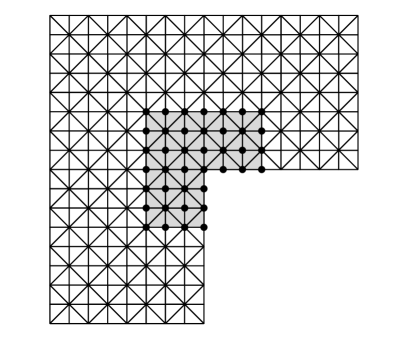
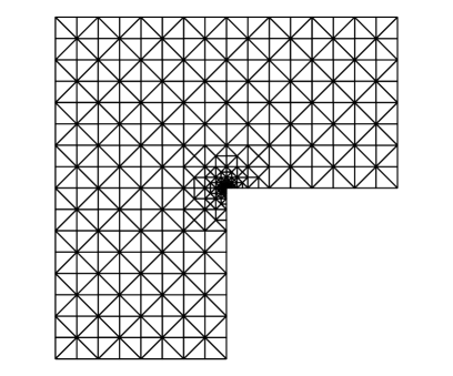
Figure 1: Sample triangulations $\mathcal{T}_{H}$ (left) and $\mathcal{T}_{h}$ (right). The shaded area in the left triangulation marks the support of functions in the kernel space $W_{h}$ (see Subsection 4.1.1).

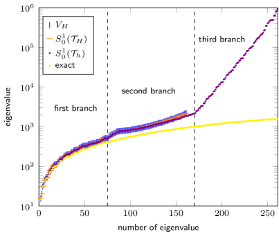
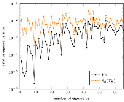
Figure 2: Spectra of finite element discretisations of the Laplacian based on the spaces $S^{1}_{0}(\mathcal{T}_{H})$, $S^{1}_{0}(\mathcal{T}_{h})$ and the generalised finite element space $V_{H}$ (left) for the triangulations from Figure 1. The exact eigenvalues of the Laplacian with homogeneous Dirichlet boundary condition are depicted for reference. On the right, the relative eigenvalue errors for the approximations in $V_{H}$ and $S^{1}_{0}(\mathcal{T}_{H})$ of the eigenvalues in $S^{1}_{0}(\mathcal{T}_{h})$ are plotted for the first branch.

We shall finally have a look at the advantageous properties of the reduced ansatz space $V_{H}$ from a different angle. Figure 2 shows the eigenvalues related to the $P_{1}$ finite element discretisation of the Laplacian with homogeneous Dirichlet boundary condition on the refined triangulation $\mathcal{T}_{h}$ depicted in Figure 1. Essentially, the spectrum consists of three branches indicated by the dotted lines. The eigenvalues in the first branch are meaningful approximations of the corresponding exact eigenvalues of the Laplacian and the corresponding eigenfunctions reflect true modes of the operator. The eigenvalues of the second and third branch are spurious in the sense that they do not approximate Laplacian eigenvalues. The artificial modes of the second branch are related to the fact that the finite element space does not satisfy $\Delta S^{1}_{0}(\mathcal{T}_{h})\subseteq L^{2}(\Omega)$ [14]. The artificial eigenvalues of the third branch are related to the degrees of freedom introduced by the local mesh refinement. The largest of them scales like the reciprocal squared minimal mesh size which leads to the restrictive CFL condition.

In a way, this restriction is the result of additional flexibility of the finite element space introduced through local mesh refinement. The role of the reduction process is to eliminate those artificial modes of the third branch while preserving the first branch extremely accurately, in particular, much more accurately than standard finite elements on the coarse mesh. That this is indeed the case is also illustrated in Figure 2 where the right plot shows that the novel subspace reduction improves the approximation of the first branch by orders of magnitude when compared with the standard finite elements $S^{1}_{0}(\mathcal{T}_{H})$ of the same dimension. The largest eigenvalues in $V_{H}$ and $S^{1}_{0}(\mathcal{T}_{H})$ are very close to each other, and therefore the CFL condition leads to almost the same restriction of the time step size. For a rigorous analysis of eigenvalue errors that justifies these observations we refer to previous works on two-level methods for linear and non-linear eigenvalue problems [16, 22, 23].

2.4 Example for $L^{2}$ and $H^{1}$ stable quasi interpolation

This subsection gives an example for a projective quasi interpolation operator $I_{H}$ that satisfies (2.5) and (2.6).

Define the space of (possibly discontinuous) piecewise affine functions over $\mathcal{T}_{H}$ as

$$P_{1}(\mathcal{T}_{H}):=\{w\in L^{2}(\Omega)\mid\forall T\in\mathcal{T}_{H}{:}\;w|_{T}\text{ is affine}\}.$$

Given $w_{H}\in P_{1}(\mathcal{T}_{H})$, define the nodal averaging operator $J_{1}:P_{1}(\mathcal{T}_{H})\to S^{1}_{0}(\mathcal{T}_{H})$ by the averaging over the values of adjacent simplices, i.e.,

$$J_{1}w_{H}(z):=(\mathrm{card}(\{K\in\mathcal{T}_{H}\mid z\in K\}))^{-1}\sum_{\begin{subarray}{c}K\in\mathcal{T}_{H}\\ z\in K\end{subarray}}w_{H}|_{K}(z)$$

for all interior nodes $z$ of $\mathcal{T}_{H}$. This kind of operator is well known in the context of fast solvers [3, 26] and in the a posteriori analysis of discontinuous Galerkin methods [21]. Let $\Pi_{1}^{\mathcal{T}_{H}}:V\to P_{1}(\mathcal{T}_{H})$ denote the $L^{2}$ projection onto $P_{1}(\mathcal{T}_{H})$ and define $I_{H}:V\to S^{1}_{0}(\mathcal{T}_{H})$ by

$$I_{H}v:=J_{1}(\Pi_{1}^{\mathcal{T}_{H}}v)\qquad\text{for all }v\in V.$$

Then $I_{H}$ is a projection. The following lemma proves that it satisfies the $L^{2}$ stability (2.6) and the approximation and stability properties (2.5).

Lemma 2.2 (stability of $I_{H}$).

The operator $I_{H}$ is $H^{1}$ and $L^{2}$ stable in the sense that it satisfies (2.5) and (2.6).

Proof.

The proof follows from the more general situation in [13], but is given here for the sake of completeness and self-contained reading.

We first prove the $L^{2}$ stability of $J_{1}:P_{1}(\mathcal{T}_{H})\to S^{1}_{0}(\mathcal{T}_{H})$ and then conclude the approximation properties and the $H^{1}$ and $L^{2}$ stability of $I_{H}$.

Let $w_{H}\in P_{1}(\mathcal{T}_{H})$ and $T=\mathrm{conv}\{z_{0},\dots,z_{d}\}\in\mathcal{T}_{H}$ and let $\lvert T\rvert$ denote the ($d$-dimensional) volume of $T$. The definition of $J_{1}$ involves adjacent simplices of $T$. For such an adjacent simplex $K$, let $\lambda_{\mathrm{max}}(T)$ and $\lambda_{\mathrm{min}}(K)$ denote the maximal and the minimal eigenvalue of the mass matrix on the simplex $T$ and $K$. The definition of $J_{1}$ then implies

$$\|J_{1}w_{H}\|_{L^{2}(T)}^{2}\leq\lambda_{\mathrm{max}}(T)\sum_{j=0}^{d}\lvert(J_{1}w_{H})(z_{j})\rvert^{2} \leq C\lambda_{\mathrm{max}}(T)\sum_{j=0}^{d}\sum_{\begin{subarray}{c}K\in\mathcal{T}_{H}\\ z_{j}\in K\end{subarray}}\big{\lvert}w_{H}|_{K}(z_{j})\big{\rvert}^{2}$$

$$\leq C\sum_{j=0}^{d}\sum_{\begin{subarray}{c}K\in\mathcal{T}_{H}\\ z_{j}\in K\end{subarray}}\frac{\lambda_{\mathrm{max}}(T)}{\lambda_{\mathrm{min}}(K)}\,\|w_{H}\|_{L^{2}(K)}^{2}.$$

The shape regularity of $\mathcal{T}_{H}$ implies that there exists a generic constant $c>0$ with $\lvert T\rvert\leq c\lvert K\rvert$ for any $K\in\mathcal{T}_{H}$ with $K\cap T\neq\emptyset$. This implies

$$\frac{\lambda_{\mathrm{max}}(T)}{\lambda_{\mathrm{min}}(K)}\leq C.$$

Therefore, $J_{1}$ satisfies a (local) $L^{2}$ stability, which together with the fact that the number of overlapping simplices is bounded leads to the $L^{2}$ stability

$$\|J_{1}w_{H}\|\leq C\|w_{H}\|.$$

Since $\Pi_{1}^{\mathcal{T}_{H}}:V\to P_{1}(\mathcal{T}_{H})$ is the $L^{2}$ projection, this operator is $L^{2}$ stable. The $L^{2}$ stability of $J_{1}$ therefore implies the $L^{2}$ stability (2.6) of $I_{H}=J_{1}\circ\Pi_{1}^{\mathcal{T}_{H}}$.

Let now $v\in V$. A triangle inequality, the fact that $\|v-\Pi_{1}^{\mathcal{T}_{H}}v\|\leq\|v-\Pi_{0}^{\mathcal{T}_{H}}v\|$ for the $L^{2}$ projection $\Pi_{0}^{\mathcal{T}_{H}}$ onto piecewise constants and a piecewise Poincaré inequality lead to

$$H^{-1}\|v-I_{H}v\| \leq H^{-1}\|v-\Pi_{1}^{\mathcal{T}_{H}}v\|+H^{-1}\|\Pi_{1}^{\mathcal{T}_{H}}v-J_{1}\Pi_{1}^{\mathcal{T}_{H}}v\|$$

$$\leq C\|\nabla v\|+H^{-1}\|\Pi_{1}^{\mathcal{T}_{H}}v-J_{1}\Pi_{1}^{\mathcal{T}_{H}}v\|.$$

Define the set of hyper-surfaces $\mathcal{F}$ and let $[\bullet]_{F}$ denote the jump across a hyper-surface $F\in\mathcal{F}$. The stability of $J_{1}$ from [5, Lemma 4.8] proves

$$H^{-2}\|\Pi_{1}^{\mathcal{T}_{H}}v-J_{1}\Pi_{1}^{\mathcal{T}_{H}}v\|^{2}\leq C\left(\|\nabla\Pi_{1}^{\mathcal{T}_{H}}v\|^{2}+\sum_{F\in\mathcal{F}}H^{-1}\|[\Pi_{1}^{\mathcal{T}_{H}}v]_{F}\|_{L^{2}(F)}^{2}\right).$$

Since $v$ is continuous in the sense of traces, the trace inequality from [9, Lemma 1.49] and the finite overlap of patches imply

$$\sum_{F\in\mathcal{F}}H^{-1}\|[\Pi_{1}^{\mathcal{T}_{H}}v]_{F}\|_{L^{2}(F)}^{2} =\sum_{F\in\mathcal{F}}H^{-1}\|[v-\Pi_{1}^{\mathcal{T}_{H}}v]_{F}\|_{L^{2}(F)}^{2}$$

$$\leq C\left(H^{-2}\|v-\Pi_{1}^{\mathcal{T}_{H}}v\|^{2}+\|\nabla(v-\Pi_{1}^{\mathcal{T}_{H}}v)\|^{2}\right).$$

Again, a piecewise Poincaré inequality bounds the first term on the right-hand side by $\|\nabla v\|$. An inverse inequality, the $L^{2}$ stability of $\Pi_{1}^{\mathcal{T}_{H}}$ and $\Pi_{1}^{\mathcal{T}_{H}}\Pi_{0}^{\mathcal{T}_{H}}v=\Pi_{0}^{\mathcal{T}_{H}}v$ prove for all $T\in\mathcal{T}_{H}$ that

$$\|\nabla\Pi_{1}^{\mathcal{T}_{H}}v\|_{L^{2}(T)} =\|\nabla(\Pi_{1}^{\mathcal{T}_{H}}v-\Pi_{0}^{\mathcal{T}_{H}}v)\|_{L^{2}(T)}\leq CH^{-1}\|\Pi_{1}^{\mathcal{T}_{H}}(v-\Pi_{0}^{\mathcal{T}_{H}}v)\|_{L^{2}(T)}$$

$$\leq CH^{-1}\|v-\Pi_{0}^{\mathcal{T}_{H}}v\|_{L^{2}(T)}\leq C\|\nabla v\|_{L^{2}(T)}.$$

The combination of the previous inequalities yield the approximation property

$$H^{-1}\|v-I_{H}v\|\leq C\|\nabla v\|$$ (2.10)

of $I_{H}$.

For the proof of the $H^{1}$ stability of $I_{H}$ let $v\in V$. An inverse, a triangle and a piecewise Poincaré inequality and the approximation property (2.10) lead to

$$\|\nabla I_{H}v\|=\|\nabla(I_{H}v-\Pi_{0}^{\mathcal{T}_{H}}v)\| \leq CH^{-1}\|I_{H}v-\Pi_{0}^{\mathcal{T}_{H}}v\|$$

$$\leq CH^{-1}\|v-I_{H}v\|+CH^{-1}\|v-\Pi_{0}^{\mathcal{T}_{H}}v\|\leq C\|\nabla v\|.$$

This proves (2.5) and concludes the proof. ∎

3 Application to the wave equation

This section defines the leapfrog discretisation of the wave equation based on the spatial Galerkin approximation in the reduced space $V_{H}$ in Subsection 3.1 and states an error estimate and stability in Subsection 3.2.

Given $f\in L^{2}(0,T;L^{2}(\Omega))$, the wave equation (1.1) in its weak form seeks $u\in L^{2}(0,T;V)$ with $\dot{u}\in L^{2}(0,T;L^{2}(\Omega))$ and $\ddot{u}\in L^{2}(0,T;H^{-1}(\Omega))$ such that for almost all $t\in[0,T]$ and all $v\in V$

$$\left\langle\ddot{u}(t),v\right\rangle_{H^{-1}(\Omega)\times H^{1}_{0}(\Omega)}+(\nabla u(t),\nabla v)_{L^{2}(\Omega)}=(f(t),v)_{L^{2}(\Omega)}.$$ (3.1)

3.1 The leapfrog in the reduced space

Let the time step size $\Delta t$ satisfy the relaxed CFL-condition

$$\Delta t<\sqrt{2}/C_{\mathrm{inv}}(V_{H})$$ (3.2)

and let $N=\lceil T/\Delta t\rceil$ be the number of time steps. Recall the definition of the space $V_{H}$ from Subsection 2.2. Given approximations $u_{H}^{0}\in V_{H}$ to $u(0)$ and $u_{H}^{1}\in V_{H}$ to $u(\Delta t)$, this method seeks $(u_{H}^{n})_{n=0,\dots,N}$ with $u_{H}^{n}\in V_{H}$ such that for all $n=2,\dots,N$ and all $v_{H}\in V_{H}$

$$\left(\frac{u_{H}^{n+1}-2u_{H}^{n}+u_{H}^{n-1}}{(\Delta t)^{2}},v_{H}\right)_{L^{2}(\Omega)}+(\nabla u_{H}^{n},\nabla v_{H})_{L^{2}(\Omega)}=\left(f(n\Delta t),v_{H}\right)_{L^{2}(\Omega)}.$$ (3.3)

This is the standard leapfrog time discretisation. We shall emphasise that the pre-computation of the space $V_{H}$ needs to be done only once.

Lemma 2.1 proves that $C_{\mathrm{inv}}(V_{H})\leq CH^{-1}$ and, hence, the CFL condition (3.2) states that the time step size is in the range of the mesh size of the (coarse) quasi-uniform triangulation $\mathcal{T}_{H}$. In the presence of singularities, this is a much weaker condition compared with the CFL condition (2.1) for the space $S^{1}_{0}(\mathcal{T}_{h})$.

One of the fundamental properties of the leapfrog scheme is the conservation of energy in the following sense. Given $(v_{H}^{n})_{n=0,\dots,N}$ with $v_{H}^{n}\in V_{H}$ for $n=0,\dots,N$, define the discrete time derivative by

$$\dot{v}_{H}^{n+1/2}=\frac{v_{H}^{n+1}-v_{H}^{n}}{\Delta t}$$

for $n=1,\dots,N-1$ and define the discrete energy as

$$\mathcal{E}^{n+1/2}((v_{H}^{k})_{k=0,\dots,N}):=\tfrac{1}{2}\big{(}\|\dot{v}^{n+1/2}_{H}\|^{2}+(\nabla v_{H}^{n},\nabla v_{H}^{n+1})\big{)}.$$

Then the discrete energy of the solution $(u_{H}^{k})_{k=0,\dots,N}$ of (3.3) is conserved in the sense that

$$\mathcal{E}^{n+1/2}((u_{H}^{k})_{k=0,\dots,N})=\mathcal{E}^{n-1/2}((u_{H}^{k})_{k=0,\dots,N})+\tfrac{1}{2}\Delta t\big{(}f(t_{n}),\dot{u}^{n+1/2}_{H}+\dot{u}^{n-1/2}_{H}\big{)}_{L^{2}(\Omega)}.$$

3.2 Stability and error estimates

The following theorem estimates the difference between the discrete solution of (3.3) and the exact solution $u$ of (3.1). Let $z_{H}\in L^{2}(0,T;V_{H})$ denote the auxiliary semi-discrete solution, i.e., $\dot{z}_{H}\in L^{2}(0,T;V_{H})$, $\ddot{z}_{H}\in L^{2}(0,T;V_{H})$ and $z_{H}$ solves

$$\left\langle\ddot{z}_{H}(t),v_{H}\right\rangle_{H^{-1}(\Omega)\times H^{1}_{0}(\Omega)}+(\nabla z_{H}(t),\nabla v_{H})_{L^{2}(\Omega)}=(f(t),v_{H})_{L^{2}(\Omega)}\quad\text{for all }v_{H}\in V_{H}$$

for almost all $t\in[0,T]$ with initial conditions $z_{H}(0)=u_{H}^{0}$ and $\dot{z}_{H}(0)=z_{H}^{0}$ for some $z_{H}^{0}$. As usual, the error is split in the time discretisation error $(E^{n})_{n=0,\dots,N}$ defined by $E^{n}:=u_{H}^{n}-z_{H}(n\Delta t)$ and the space discretisation error $z_{H}(n\Delta t)-u(n\Delta t)=z_{H}(n\Delta t)-\Pi_{V_{H}}u(n\Delta t)-\varepsilon(n\Delta t)$ with the best-approximation error $\varepsilon(t):=u(t)-\Pi_{V_{H}}u(t)$, where $\Pi_{V_{H}}u(t)$ denotes the orthogonal projection of $u(t)$ onto $V_{H}$ with respect to the bilinear form $(\nabla\bullet,\nabla\bullet)_{L^{2}(\Omega)}$.

The proof of the following theorem is based on the conservation of the discrete energy from Subsection 3.1 and follows as for the standard leapfrog scheme (see [6, 20]) and is therefore dropped.

Theorem 3.1 (error estimate for reduced FEM).

If the relaxed CFL condition (3.2) is satisfied, then (3.3) is stable in the sense that

$$\|\dot{u}_{H}^{n+1/2}\|+\|\nabla u_{H}^{n+1}\|\leq C\left(\|\dot{u}_{H}^{1/2}\|+\|\nabla u_{H}^{0}\|+\|\nabla u_{H}^{1}\|+\sum_{k=2}^{n}\Delta t\|f(k\Delta t)\|\right).$$

Furthermore, if $\ddot{u}\in L^{1}(0,T;L^{2}(\Omega))$ and $\ddot{z}_{H}\in C(0,T;V_{H})$, then it holds with $t_{n}=n\Delta t$ that

$$\left\|\frac{(u_{H}^{n}-u(t_{n}))-(u_{H}^{n-1}+u(t_{n-1}))}{\Delta t}\right\|+\|\nabla(u_{H}^{n}-u(t_{n}))\|$$ (3.4)

$$\;\leq C\left(\|\dot{E}^{1/2}\|+\|\nabla E^{1}\|+\left\|\dot{z}_{H}(0)-\Pi_{V_{H}}\dot{u}(0)\right\|+\|\nabla(z_{H}(0)-\Pi_{V_{H}}u(0)\|\right.$$

$$\qquad\qquad\;\left.+\left\|\frac{\varepsilon(t_{n})-\varepsilon(t_{n-1})}{\Delta t}\right\|+\|\nabla\varepsilon(t_{n})\|+\int_{0}^{t_{n}}\left\|\ddot{\varepsilon}(s)\right\|\,ds\right.$$

$$\qquad\qquad\;\left.+\sum_{j=1}^{n}\Delta t\left\|\frac{z_{H}(t_{j+1})-2z_{H}(t_{j})+z_{H}(t_{j-1})}{(\Delta t)^{2}}-\ddot{z}_{H}(t_{j})\right\|\right).$$

Note that the fifth to seventh term on the right-hand side of (3.4) only contain the best-approximation error $\varepsilon$ of $u$ in $V_{H}$. Therefore, Lemma 2.1 can be applied. If $u\in C^{2}(0,T;L^{2}(\Omega))$ and $f\in C(0,T;L^{2}(\Omega))$, then $\Delta u=\ddot{u}-f\in C^{0}(0,T;L^{2}(\Omega))$, and the term $\|\Delta u\|_{L^{2}(\Omega)}$ in the right-hand side of (2.9) is bounded. Therefore, under the additional (standard) regularity assumptions $u\in C^{4}(0,T;L^{2}(\Omega))$ and $f\in C^{2}(0,T;L^{2}(\Omega))$, the fifth to seventh term can be bounded by $H$. With the regularity assumption $z_{H}\in C^{4}(0,T;L^{2}(\Omega))$, the last term on the right-hand side of (3.4) converges as $(\Delta t)^{2}$. For suitable initial conditions, this leads to a convergence rate of the approximation (3.3) of $H+(\Delta t)^{2}$.

4 Practical aspects and possible generalisations

This section is concerned with practical aspects of the computation of $(u_{H}^{n})_{n=0,\dots,N}$ from (3.3). Subsection 4.1 discusses the sparsity properties of the stiffness and mass matrix associated with the reduced space $V_{H}$. Since the computation of $V_{H}$ has to be done only once, the sparsity properties serve as measure for the overall complexity. Subsection 4.2 shows that the inverse diagonal is an optimal preconditioner for the mass matrix of the reduced space. Subsection 4.3 concludes this section with a generalisation to discontinuous Galerkin FEMs.

4.1 Sparsity of the reduced space

In contrast to standard finite element spaces, basis functions of $V_{H}$ are not a priori known, but can be defined by the canonical choice $\lambda_{z}-\mathcal{C}\lambda_{z}$ for the standard nodal basis functions $\lambda_{z}$ of $S^{1}_{0}(\mathcal{T}_{H})$. However, problem (2.7) for the computation of $\mathcal{C}\lambda_{z}$ is formulated on the whole domain $\Omega$, and might lead to global basis functions and dense stiffness and mass matrices. This subsection identifies cases where sparsity is automatically preserved (Subsection 4.1.1) and shows how to achieve sparse approximations in the general case (Subsection 4.1.2).

4.1.1 Sparsity on locally adaptive meshes

We consider the case that the triangulation $\mathcal{T}_{h}$ refines $\mathcal{T}_{H}$ only locally in the sense that only a small number of coarse elements is actually refined, for an example see Figure 1. In this case the corrector problem (2.7) reduces to a local one because the kernel space $W_{h}$ vanishes outside of (one layer around) the refined region (see the following proposition). Therefore, $\mathcal{C}\lambda_{z}=0$ for all basis functions $\lambda_{z}$ for nodes $z$ of $\mathcal{T}_{H}$ with the property that the two-layer patch

$$\Omega_{z}:=\{x\in\Omega\mid\exists T,T^{\prime}\in\mathcal{T}_{H}\text{ such that }z\in T,x\in T^{\prime}\text{ and }T\cap T^{\prime}\neq\emptyset\}$$

lies in the non-refined region, $\Omega_{z}\subseteq\bigcup(\mathcal{T}_{H}\cap\mathcal{T}_{h})$. In the example of Figure 1, all nodes $z$ for which $\mathcal{C}\lambda_{z}\neq 0$ are highlighted as well as the union of the supports of functions in $W_{h}$.

Proposition 4.1 (locality of problems (2.7)).

Assume that $I_{H}$ satisfies the local $L^{2}$ stability

$$\|I_{H}v\|_{L^{2}(T)}\leq C\|v\|_{L^{2}(\Omega_{T})}\qquad\text{for all }v\in V$$

for all $T\in\mathcal{T}_{H}$ and $\Omega_{T}=\bigcup\{K\in\mathcal{T}_{H}\mid K\cap T\neq\emptyset\}$. Let $w_{h}\in W_{h}$. Then $w_{h}|_{\widetilde{\Omega}}=0$ for $\widetilde{\Omega}=\bigcup\{T\in\mathcal{T}_{H}\mid\forall K\in\mathcal{T}_{H}\text{ with }K\cap T\neq\emptyset\text{ it holds }K\in\mathcal{T}_{H}\cap\mathcal{T}_{h}\}$.

Proof.

Let $\mathcal{N}$ denote the set of nodes in $\mathcal{T}_{h}$ that are not in $\mathcal{T}_{H}$ and define $w_{y}:=\lambda_{y}-I_{H}\lambda_{y}$ for $y\in\mathcal{N}$. We want to show that the functions $w_{y}$ for $y\in\mathcal{N}$ are linear independent. Let $\alpha_{y}\in\mathbb{R}$ such that

$$\sum_{y\in\mathcal{N}}\alpha_{y}w_{y}=0.$$

On the one hand, the definition of $w_{y}$ leads to $\sum_{y\in\mathcal{N}}\alpha_{y}\lambda_{y}=\sum_{y\in\mathcal{N}}\alpha_{y}I_{H}\lambda_{y}\in S^{1}_{0}(\mathcal{T}_{H})$, i.e., the function $\sum_{y\in\mathcal{N}}\alpha_{y}\lambda_{y}$ is piecewise affine on the triangulation $\mathcal{T}_{H}$. On the other hand, the functions $\lambda_{y}$ vanish at all nodes in $\mathcal{T}_{H}$. This implies that the functions $w_{y}$ are linear independent. A dimension argument proves that they form a basis of $W_{h}$. The local $L^{2}$ stability implies that $w_{y}$ has the local support $\{x\in\Omega\mid\exists T,T^{\prime}\in\mathcal{T}_{H}\text{ such that }x\in T,y\in T^{\prime}\text{ and }T\cap T^{\prime}\neq\emptyset\}$. ∎

Proposition 4.1 implies that the number of additional non-zero entries in the mass and stiffness matrix depends only on the number of triangles of $\mathcal{T}_{H}$ that are refined in $\mathcal{T}_{h}$.

4.1.2 Sparsification on graded meshes

In this subsection we consider an arbitrary refinement $\mathcal{T}_{h}$ of $\mathcal{T}_{H}$. Given a coarse nodal basis function $\lambda_{z}$, it was shown in [24] that $\mathcal{C}\lambda_{z}$ decays exponentially fast outside of the support of $\lambda_{z}$ (see [27] for illustrations). This decay allows the truncation of the computational domain for (2.7) to local subdomains of diameter $mH$, roughly, where $m$ denotes a new discretisation parameter, namely the localisation or oversampling parameter. The obvious way would be to simply replace the global domain $\Omega$ in the computation of $\mathcal{C}\lambda_{z}$ with suitable neighbourhoods of the nodes $z$. This procedure was used in [24]. However, it turned out that it is advantageous to consider the following slightly more involved technique based on element correctors [18, 17]. Define the $m$-th order patch

$$\Omega_{T,m}:=\bigcup\left\{K\in\mathcal{T}_{H}\left|\begin{array}[]{l}\exists K_{0},\dots,K_{m}\in\mathcal{T}_{H}\text{ with }K_{0}=T,K_{m}=K\\ \text{ and }K_{j}\cap K_{j+1}\neq\emptyset\text{ for all }j=0,\dots,m-1\end{array}\right.\right\}.$$

We introduce corresponding truncated function spaces

$$W_{h}(\Omega_{T,m}):=\{w_{h}\in W_{h}\mid\mathrm{supp}(w_{h})\subseteq\Omega_{T,m}\}.$$

Given any coarse nodal basis function $\lambda_{z}\in S^{1}_{0}(\mathcal{T}_{H})$, let $\mathcal{C}_{T,m}\lambda_{z}\in W_{h}(\Omega_{T,m})$ solve the localised element problem

$$(\nabla w_{h},\nabla\mathcal{C}_{T,m}\lambda_{z})_{L^{2}(\Omega)}=\int_{T}\nabla w_{h}\cdot\nabla\lambda_{z}\quad\text{for all }w_{h}\in W_{h}(\Omega_{T,m})$$

and define $\mathcal{C}_{m}\lambda_{z}:=\sum_{T\in\mathcal{T}_{H}}\mathcal{C}_{T,m}\lambda_{z}$. Note that we impose homogeneous Dirichlet boundary conditions on the artificial boundary of the patch $\Omega_{T,m}$ which is well justified by the fast decay. Under the assumption that $\mathcal{T}_{h}$ is shape regular and that $I_{H}$ is a local operator (as the one introduced in Subsection 2.4) it is proved in [18, 24, 17] that this leads to the existence of constants $C>0$ and $\beta>0$ such that

$$\|\nabla(\mathcal{C}\lambda_{z}-\mathcal{C}_{m}\lambda_{z})\|\leq C\exp(-\beta m)\|\nabla\lambda_{z}\|.$$ (4.1)

This justifies the utilisation of

$$V_{H}^{(m)}:=\mathrm{span}\{\lambda_{z}-\mathcal{C}_{m}\lambda_{z}\mid z\text{ interior node of }\mathcal{T}_{H}\}$$

as an approximation to $V_{H}$. Due to the exponential decay (4.1), the choice of $m\approx\lvert\log(H)\rvert$ ensures that this perturbation does not affect the advantageous approximation properties of $V_{H}$.

For the construction of the basis, $O(H^{-d})$ problems have to be solved. Each of these problems consists of $O((\log(H)H/h_{\mathrm{min}})^{d})$ degrees of freedoms in the worst case, depending on the grading of the fine triangulation. These costs are offline costs in the sense that the basis has to be constructed in the beginning only and does not depend on the number of time steps. It does only depend on the coarse and the fine mesh. The non-zero entries in the mass and stiffness matrix amount to $O((2\log(H)/H)^{d})$.

4.2 Diagonal preconditioning of the mass matrix

This subsection proves that the inverse of the diagonal of the mass matrix is a suitable preconditioner for it. Although this is shown for $V_{H}$ with basis functions $\lambda_{z}-\mathcal{C}\lambda_{z}$, the arguments and therefore also the result hold as well for the perturbed spaces $V_{H}^{(m)}$ of Subsection 4.1.2 spanned by the local basis functions $\lambda_{z}-\mathcal{C}_{m}\lambda_{z}$.

Define $D:=\mathrm{dim}(S^{1}_{0}(\mathcal{T}_{H}))$. Let $(\Lambda_{k})_{k=1,\dots,D}$ denote the basis of $S^{1}_{0}(\mathcal{T}_{H})$ consisting of the standard nodal basis functions. Then $(\lambda_{k})_{k=1,\dots,D}$ with $\lambda_{k}=(1-\mathcal{C})\Lambda_{k}$ for $\mathcal{C}$ from (2.7) defines a basis of $V_{H}$. Let $\mathcal{M}$ and $M$ denote the mass matrices with respect to $(\Lambda_{k})_{k=1,\dots,D}$ and $(\lambda_{k})_{k=1,\dots,D}$. Let $x\in\mathbb{R}^{D}$ and let

$$U_{H}:=\sum_{k=1}^{D}x_{k}\Lambda_{k}\in S^{1}_{0}(\mathcal{T}_{H})\qquad\text{and}\qquad u_{H}:=\sum_{k=1}^{D}x_{k}\lambda_{k}=(1-\mathcal{C})U_{H}\in V_{H}$$

denote the corresponding functions in $S^{1}_{0}(\mathcal{T}_{H})$ and $V_{H}$. Then,

$$x^{\top}Mx=\|u_{H}\|^{2}=\|(1-\mathcal{C})U_{H}\|^{2}\leq(\|U_{H}\|+\|\mathcal{C}U_{H}\|)^{2}.$$

Since $\mathcal{C}U_{H}\in W_{h}$, the approximation properties (2.5) and the inverse inequality (2.3) imply

$$\|U_{H}\|+\|\mathcal{C}U_{H}\| \leq\|U_{H}\|+C_{I_{H}}^{(1)}H\|\nabla U_{H}\|\leq\left(1+C_{I_{H}}^{(1)}HC_{\mathrm{inv}}(S^{1}_{0}(\mathcal{T}_{H}))\right)\|U_{H}\|$$

$$=\left(1+C_{I_{H}}^{(1)}HC_{\mathrm{inv}}(S^{1}_{0}(\mathcal{T}_{H}))\right)\sqrt{x^{\top}\mathcal{M}x}.$$

On the other hand, since $U_{H}=I_{H}u_{H}$, the $L^{2}$ stability (2.6) leads to

$$\sqrt{x^{\top}\mathcal{M}x}=\|U_{H}\|\leq C_{I_{H}}^{(0)}\|u_{H}\|=C_{I_{H}}^{(0)}\,\sqrt{x^{\top}Mx}.$$

Given $A,B\in\mathbb{R}$, let $A\approx B$ abbreviate that there exist generic constants $C_{1}>0$, $C_{2}>0$ independent of the mesh size, such that $A\leq C_{1}B\leq C_{2}A$. Since $C_{\mathrm{inv}}(S^{1}_{0}(\mathcal{T}_{H}))\approx H^{-1}$, the above result reads

$$x^{\top}Mx\approx x^{\top}\mathcal{M}x.$$

Since this result also holds for the unit vectors $e_{j}\in\mathbb{R}^{D}$, this implies

$$x^{\top}\mathrm{diag}(\mathcal{M})x=\sum_{j=1}^{D}x_{j}^{2}e_{j}^{\top}\mathcal{M}e_{j}\approx\sum_{j=1}^{D}x_{j}^{2}e_{j}^{\top}Me_{j}=x^{\top}\mathrm{diag}(M)x.$$

Since $x^{\top}\mathrm{diag}(\mathcal{M})x\approx x^{\top}\mathcal{M}x$ [30], it follows

$$x^{\top}\mathrm{diag}(M)x\approx x^{\top}\mathrm{diag}(\mathcal{M})x\approx x^{\top}\mathcal{M}x\approx x^{\top}Mx.$$

Therefore, $(\mathrm{diag}(M))^{-1}$ is a suitable preconditioner for $M$ and the application of $M^{-1}$ may be replaced with a few iterations of the preconditioned conjugate gradient method.

4.3 Generalisation to other FEMs

The reduction approach is not at all restricted to linear conforming finite elements. The generalisation to many non-standard schemes is possible. If one considers, e.g., a discontinuous Galerkin discretisation instead of a FEM approximation, then $I_{H}=\Pi_{\mathrm{dG}}$ the $L^{2}$ projection onto the discontinuous Galerkin space satisfies the approximation properties (2.5) and the $L^{2}$ stability (2.6) with $\|\nabla\bullet\|$ replaced by the dG norm

$$\sqrt{\sum_{T\in\mathcal{T}_{h}}\|\nabla\bullet\|_{L^{2}(T)}^{2}+\sum_{F\in\mathcal{F}}\frac{\sigma}{\mathrm{diam}(F)}\|[\bullet]_{F}\|_{L^{2}(F)}^{2}},$$

where $\mathcal{F}$ denotes the set of hyper-surfaces of $\mathcal{T}_{h}$ (e.g., the set of edges for $d=2$ and the set of faces for $d=3$), $[\bullet]_{F}$ denotes the jump across a hyper-surfaces $F$ and $\sigma$ is some penalty parameter. Furthermore, Lemma 2.1 holds equally with this choice of quasi-interpolation. In the context of numerical homogenisation, the reduced space for discontinuous Galerkin discretisations was utilised in [12].

Higher order elements are also possible in principal, if $\Delta u$ is sufficiently smooth. The design of a suitable interpolation operator $I_{H}$ with additional properties is crucial: Additional orthogonality properties have to ensure that the term $(-\Delta u,e_{h})_{L^{2}(\Omega)}$ with $e_{h}\in\mathrm{ker}(I_{H}|_{S^{1}_{0}(\mathcal{T}_{h})})$ in the proof of Lemma 2.1 converges with the correct rate.

5 Numerical experiment

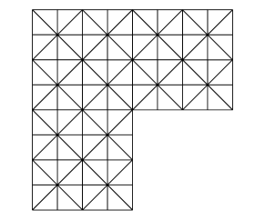
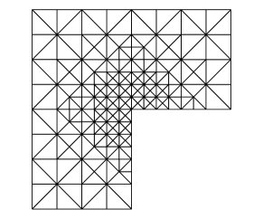
Figure 3: Triangulations $\mathcal{T}_{H,1}$ and $\mathcal{T}_{h,1}$ for the numerical experiment from Section 5.

In this example we consider the wave equation (1.1) on the spatial L-shaped domain $\Omega:=(-1,1)^{2}\setminus([0,1]\times[-1,0])\subseteq\mathbb{R}^{2}$ for the time interval $[0,0.5]$ with inhomogeneous Dirichlet boundary conditions $u|_{\partial\Omega}$ and right-hand side $f$ and initial conditions $u(0)$ and $\dot{u}(0)$ given by the exact singular solution

$$u(t,x)=\sin(\pi t)\,(r(x))^{2/3}\,\sin(2k\theta(x)/3)$$

in polar coordinates $(r,\theta)$. The discretisation (3.3) can naturally be generalised to this case of inhomogeneous Dirichlet boundary conditions.

We consider a sequence of uniform triangulations $(\mathcal{T}_{H,\ell})_{\ell=1,\dots,10}$, such that $\mathcal{T}_{H,\ell+1}$ is created from $\mathcal{T}_{H,\ell}$ by a proper bisection of every triangle (i.e., the longest edge in a triangle is bisected). The sequence $(\mathcal{T}_{h,\ell})_{\ell=1,\dots,10}$ consists of triangulations such that $\mathcal{T}_{h,\ell}$ is a refinement of $\mathcal{T}_{H,\ell}$ created similar as in the algorithm threshold from [15], i.e., $\mathcal{T}_{h,\ell}$ is graded towards the re-entrant corner $(0,0)$. The first triangulations $\mathcal{T}_{H,1}$ and $\mathcal{T}_{h,1}$ are depicted in Figure 3. These triangulations define the finite element spaces $S^{1}_{0}(\mathcal{T}_{H})$, $S^{1}_{0}(\mathcal{T}_{h})$. Let $I_{H,\ell}:=J_{1}\circ\Pi_{1}^{\mathcal{T}_{H,\ell}}$ as in Subsection 2.4. This defines $V_{H}$. The time step size $\Delta t$ for the standard leapfrog FEM on $S^{1}_{0}(\mathcal{T}_{H})$ and the reduced FEM from (3.3) (resp. $\Delta t_{h}$ for the standard leapfrog FEM on $S^{1}_{0}(\mathcal{T}_{h})$) is defined by

$$\Delta t:=\sqrt{2}/C_{\mathrm{inv}}(S^{1}_{0}(\mathcal{T}_{H}))\qquad(\text{resp.\ }\;\Delta t_{h}:=\sqrt{2}/C_{\mathrm{inv}}(S^{1}_{0}(\mathcal{T}_{h}))).$$ (5.1)

These time step sizes are summarised in Table 1 for the triangulations $(\mathcal{T}_{H,\ell})_{\ell=1,\dots,10}$ and $(\mathcal{T}_{h,\ell})_{\ell=1,\dots,10}$.

$\ell$	1	2	3	4	5	6	7	8	9	10	11
$\Delta t$	1.9e-2	1.3e-2	9.8e-3	6.9e-3	4.9e-3	3.4e-3	2.4e-3	1.7e-3	1.2e-3	8.6e-4	6.1e-4
$\Delta t_{h}$	6.5e-3	3.4e-3	1.6e-3	5.7e-4	4.0e-4	2.1e-4	1.0e-4	3.7e-5	2.6e-5

Table 1: Time-step sizes for uniform triangulations $\mathcal{T}_{H}$ and refined triangulations $\mathcal{T}_{h}$ defined by (5.1). The small time-step sizes $\Delta t_{h}$ limit the feasible computations of a solution of the standard leapfrog FEM on $S^{1}_{0}(\mathcal{T}_{h})$ to the first nine levels.

While $\Delta t$ is only moderately small for all considered triangulations, the fine time step-size $\Delta t_{h}$ decreases with higher rate, such that 50 times more time steps are needed for the leapfrog on $S^{1}_{0}(\mathcal{T}_{h})$ compared with $S^{1}_{0}(\mathcal{T}_{H})$ for $\ell=9$. The approximation $V_{H}^{(m)}$ of $V_{H}$ from Subsection 4.1.2 is employed in the numerical computations with $m=\lceil-0.5\log_{2}(H)\rceil$, which implies $1\leq m\leq 3$ for the performed computations. The inversions of the mass matrices $M$ are performed with the preconditioned conjugate gradients method with preconditioner $\mathrm{diag}(M)^{-1}$.

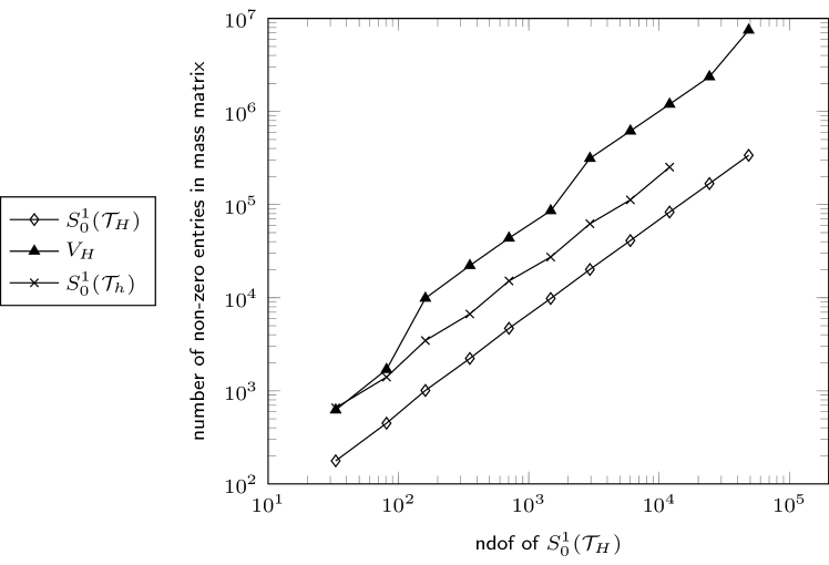
Figure 4: Number of non-zero entries in the mass matrices.

The number of non-zero entries in the mass matrices are plotted in Figure 4 and serve as a measure of the complexity. The errors

$$\sum_{k=1}^{N}\Delta t\left\|\nabla(u(k\Delta t)-U^{k})\right\|$$ (5.2)

for the discrete solution $(U^{k})_{k=1,\dots,N}$ of the reduced FEM of (3.3), of the standard leapfrog FEM on $S^{1}_{0}(\mathcal{T}_{H})$ (i.e., (3.3) with $V_{H}$ replaced by the coarse FEM space $S^{1}_{0}(\mathcal{T}_{H})$), and of the standard leapfrog FEM on $S^{1}_{0}(\mathcal{T}_{h})$ (with $\Delta t$ replaced with the fine time step size $\Delta t_{h}$ and $N$ replaced by $\lceil T/\Delta t_{h}\rceil$) serve as approximations for the error in $L^{2}(0,T;H^{1}_{0}(\Omega))$ and are plotted in Figure 5 against the number of degrees of freedom (ndof) in $S^{1}_{0}(\mathcal{T}_{H})$ (which equals the number of degrees of freedom in $V_{H}$).

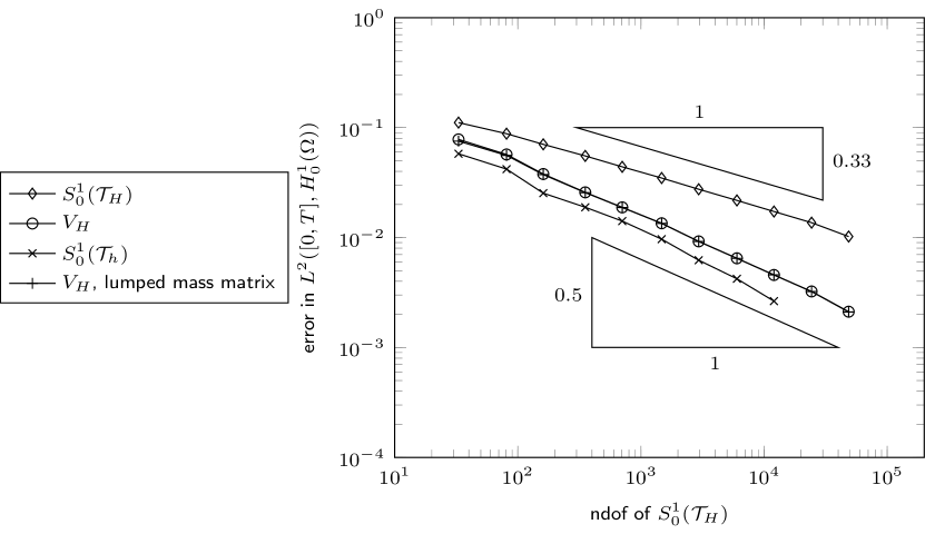
Figure 5: Errors (5.2) for the example from Section 5

The error for the standard leapfrog FEM for $S^{1}_{0}(\mathcal{T}_{H})$, i.e., on uniform triangulations, shows a suboptimal convergence rate of $\mathrm{ndof}^{1/3}\approx H^{2/3}$, while the approximation with (3.3) and the standard leapfrog FEM on $S^{1}_{0}(\mathcal{T}_{h})$ yield the optimal convergence rate of $\mathrm{ndof}^{1/2}$ as predicted by Theorem 3.1. Figure 5 also contains the errors of the leapfrog FEM for $V_{H}$ with the mass matrix replaced by the lumped mass matrix, i.e., the diagonal matrix whose entry $M_{jj}$ equals the sum of the row entries $(M_{jk})_{k=1,\dots,\mathrm{dim}(V_{H})}$. The error shows the same behaviour as without mass lumping.

Due to the small time step sizes, implicit schemes were previously employed for numerical experiments on adaptive meshes [25], which require the expensive inversion of the stiffness matrix in every time step. The reduced space $V_{H}$ overcomes the restrictive CFL condition and turns the leapfrog into a practicable scheme: At the expense of a moderately increased complexity, the optimal convergence rate is recovered, but with the same time step sizes as for uniform meshes.

References

• [1] Abdulle, A., Henning, P.: Localized orthogonal decomposition method for the wave equation with a continuum of scales. Math. Comp. 86(304), 549–587 (2017).
• [2] Bank, R.E., Dupont, T.: An optimal order process for solving finite element equations. Math. Comp. 36(153), 35–51 (1981).
• [3] Brenner, S.C.: Two-level additive Schwarz preconditioners for nonconforming finite element methods. Math. Comp. 65(215), 897–921 (1996)
• [4] Brenner, S.C., Scott, L.R.: The Mathematical Theory of Finite Element Methods, Texts in Applied Mathematics, vol. 15, 3 edn. Springer Verlag, New York, Berlin, Heidelberg (2008)
• [5] Carstensen, C., Gallistl, D., Schedensack, M.: $L^{2}$ best-approximation of the elastic stress in the Arnold-Winther FEM. IMA J. Numer. Anal. 36(3), 1096–1119 (2016).
• [6] Christiansen, S.H.: Foundations of finite element methods for wave equations of Maxwell type. In: E. Quak, T. Soomere (eds.) Applied wave mathematics, pp. 335–393. Springer, Berlin (2009)
• [7] Ciarlet Jr., P., He, J.: The singular complement method for 2d scalar problems. C. R. Math. Acad. Sci. Paris 336(4), 353–358 (2003).
• [8] Courant, R., Friedrichs, K., Lewy, H.: Über die partiellen Differenzengleichungen der mathematischen Physik. Math. Ann. 100(1), 32–74 (1928).
• [9] Di Pietro, D.A., Ern, A.: Mathematical aspects of discontinuous Galerkin methods, Mathématiques & Applications (Berlin) [Mathematics & Applications], vol. 69. Springer, Heidelberg (2012).
• [10] Diaz, J., Grote, M.J.: Energy conserving explicit local time stepping for second-order wave equations. SIAM J. Sci. Comput. 31(3), 1985–2014 (2009).
• [11] Diaz, J., Grote, M.J.: Multi-level explicit local time-stepping methods for second-order wave equations. Comput. Methods Appl. Mech. Engrg. 291, 240–265 (2015).
• [12] Elfverson, D., Georgoulis, E.H., Målqvist, A., Peterseim, D.: Convergence of a discontinuous galerkin multiscale method. SIAM J. Numer. Anal. 51(6), 3351–3372 (2013).
• [13] Ern, A., Guermond, J.L.: Finite element quasi-interpolation and best approximation. ArXiv e-prints (2015). Preprint, arXiv:1505.06931
• [14] Gallistl, D., Huber, P., Peterseim, D.: On the stability of the Rayleigh-Ritz method for eigenvalues (2015). INS Preprint No. 1527, available at http://peterseim.ins.uni-bonn.de/research/pub/INS1527.pdf
• [15] Gaspoz, F.D., Morin, P.: Convergence rates for adaptive finite elements. IMA J. Numer. Anal. 29(4), 917–936 (2009).
• [16] Henning, P., Målqvist, A., Peterseim, D.: Two-level discretization techniques for ground state computations of Bose-Einstein condensates. SIAM J. Numer. Anal. 52(4), 1525–1550 (2014).
• [17] Henning, P., Morgenstern, P., Peterseim, D.: Multiscale partition of unity. In: M. Griebel, M.A. Schweitzer (eds.) Meshfree Methods for Partial Differential Equations VII, Lecture Notes in Computational Science and Engineering, vol. 100, pp. 185–204. Springer International Publishing (2015)
• [18] Henning, P., Peterseim, D.: Oversampling for the multiscale finite element method. Multiscale Model. Simul. 11(4), 1149–1175 (2013).
• [19] Hochbruck, M., Sturm, A.: Error analysis of a second order locally implicit method for linear Maxwell’s equations (2015). CRC 1173-Preprint, no. 2015/1, Karlsruher Institut für Technologie, available at http://www.waves.kit.edu/downloads/CRC1173_Preprint_2015-1.pdf
• [20] Joly, P.: Variational methods for time-dependent wave propagation problems. In: Topics in computational wave propagation, Lect. Notes Comput. Sci. Eng., vol. 31, pp. 201–264. Springer, Berlin (2003)
• [21] Karakashian, O.A., Pascal, F.: A posteriori error estimates for a discontinuous Galerkin approximation of second-order elliptic problems. SIAM J. Numer. Anal. 41(6), 2374–2399 (2003)
• [22] Målqvist, A., Peterseim, D.: Generalized finite element methods for quadratic eigenvalue problems. ESAIM Math. Model. Numer. Anal. 51(1), 147–163 (2016).
• [23] Målqvist, A., Peterseim, D.: Computation of eigenvalues by numerical upscaling. Numer. Math. 130(2), 337–361 (2014).
• [24] Målqvist, A., Peterseim, D.: Localization of elliptic multiscale problems. Math. Comp. 83(290), 2583–2603 (2014).
• [25] Müller, F.L., Schwab, C.: Finite elements with mesh refinement for wave equations in polygons. J. Comput. Appl. Math. 283, 163–181 (2015).
• [26] Oswald, P.: On a BPX-preconditioner for P1 elements. Computing 51(2), 125–133 (1993).
• [27] Peterseim, D.: Variational multiscale stabilization and the exponential decay of fine-scale correctors (2015). Preprint, arXiv:1505.07611
• [28] Scott, L.R., Zhang, S.: Finite element interpolation of nonsmooth functions satisfying boundary conditions. Math. Comp. 54(190), 483–493 (1990).
• [29] Verfürth, R.: A Review of a Posteriori Error Estimation and Adaptive Mesh-Refinement Techniques. Advances in numerical mathematics. Wiley (1996)
• [30] Wathen, A.J.: Realistic eigenvalue bounds for the Galerkin mass matrix. IMA Journal of Numerical Analysis 7(4), 449–457 (1987).