Approximating the $k$-Level in Three-Dimensional Plane Arrangements

Abstract

Let $H$ be a set of $n$ non-vertical planes in three dimensions, and let $r<n$ be a parameter. We give a simple alternative proof of the existence of an $O(1/r)$-cutting of the first $n/r$ levels of ${\cal A}(H)$, which consists of $O(r)$ semi-unbounded vertical triangular prisms. The same construction yields an approximation of the $(n/r)$-level by a terrain consisting of $O(r/{\varepsilon}^{3})$ triangular faces, which lies entirely between the levels $n/r$ and $(1+{\varepsilon})n/r$. The proof does not use sampling, and exploits techniques based on planar separators and various structural properties of levels in three-dimensional arrangements and of planar maps. The proof is constructive, and leads to a simple randomized algorithm, that computes the approximating terrain in $O(n+r{\varepsilon}^{-6}\log^{3}r)$ expected time. An application of this technique allows us to mimic and extend Matoušek’s construction of cuttings in the plane [Mat90], to obtain a similar construction of a “layered” $(1/r)$-cutting of the entire arrangement ${\cal A}(H)$, of optimal size $O(r^{3})$. Another application is a simplified optimal approximate range counting algorithm in three dimensions, competing with that of Afshani and Chan [AC09a].

1 Introduction

A tribute to Jirka Matoušek.

We were very fortunate to have Jirka as a friend and colleague. He has entered our community in the late 1980’s, and has been a giant lighthouse ever since, showing us the way into new discoveries, solving mysteries for us, and just providing us with new tools, ideas, and techniques, that have made our work much more interesting and productive. He has been everywhere, making seminal contributions to so many topics in computational and discrete geometry (and to other fields too). We have been avid readers of his many books, most notably Lectures on Discrete Geometry, and have been admiring his clear yet precise style of exposition and presentation. We have also learned to appreciate his personality, his dry but touching sense of humor, his love for nature, his infinite devotion to science on one hand, and to his family and friends on the other hand. His departure has been painful to us, and we will miss him badly. We thank you, Jirka, for all the gifts you gave us, and may your soul be blessed.

This paper is about a topic that Jirka has worked on, rather extensively, during the early 1990s, concerning cuttings and related techniques for decompositions of arrangements or of point sets, and their applications to range searching and other algorithmic and combinatorial problems in geometry. In particular, in 1992 he has written a seminal paper on “Reporting points in halfspaces” [Mat92c], where he introduced and analyzed shallow cuttings, a technique that had many applications during the following decades.

In a later paper, following his earlier work [Mat90] (probably his first entry into computational geometry), Jirka [Mat98] presented a construction of $(1/r)$-cuttings, for a set of lines in the plane, with $\leq 8r^{2}+6r+4$ cells. This construction uses, as a basic building block, a strikingly simple procedure for approximating a level in a line arrangement: Since a specific level is an $x$-monotone polygonal chain, one can pick every $q$-th vertex, for $q\approx n/r$, and connect these vertices consecutively to form an approximate level, which is at crossing distance at most $q/2$ from the original level. As is well known, this construction is asymptotically optimal for any arrangement of lines in general position. This elegant level approximation algorithm, in two dimensions, raises the natural question of whether one can approximate a level in three dimensions for a given set of planes, by an $xy$-monotone polyhedral terrain constructed directly, in an analogous manner, from the original level.

This paper provides an affirmative answer to this question, thereby pushing Jirka’s work further, for the special case of three-dimensional arrangements of planes. It refines the shallow cuttings technique of [Mat92c], and applies it to obtain cleaner and more efficient solutions for several related problems. Our new scheme for approximating a level by a terrain, while significantly more involved than Jirka’s two-dimensional construction, still echoes and generalizes his basic idea of “shortcutting” the original level by a coarser triangular mesh (instead of a simplified polygonal chain) spanned by selected vertices of the level.

Cuttings.

Let $H$ be a set of $n$ (non-vertical) hyperplanes in $\mathbb{R}^{d}$, and let $r<n$ be a parameter. A $(1/r)$-cutting of the arrangement ${\cal A}(H)$ is a collection of pairwise openly disjoint simplices (or other regions of constant complexity) such that the closure of their union covers $\mathbb{R}^{d}$, and each simplex is crossed (meets in its interior) at most $n/r$ hyperplanes of $H$.

Cuttings have proved to be a powerful tool for a variety of problems in discrete and computational geometry, because they provide an effective divide-and-conquer mechanism for tackling such problems; see Agarwal [Aga91a] for an early survey. Applications include a variety of range searching techniques [AE99], partition trees [Mat92a], incidence problems involving points and lines, curves, and surfaces [CEG⁺90], and many more.

The first (albeit suboptimal) construction of cuttings is due to Clarkson [Cla87]. This concept was formalized later on by Chazelle and Friedman [CF90], who gave a sampling-based construction of optimal-size cuttings (see below). An optimal deterministic construction algorithm was provided by Chazelle [Cha93]. Matoušek [Mat98] studied the number of cells in a $(1/r)$-cutting in the plane (see also [Har00]). See Agarwal and Erickson [AE99] and Chazelle [Cha04] for comprehensive reviews of this topic.

To be effective, it is imperative that the number of simplices in the cutting be asymptotically as small as possible. Chazelle and Friedman [CF90] were the first to show the existence of a $(1/r)$-cutting of the entire arrangement of $n$ hyperplanes in $\mathbb{R}^{d}$, consisting of $O(r^{d})$ simplices, which is asymptotically the best possible bound. (We note in passing that cuttings of optimal size are not known for arrangements of (say, constant-degree algebraic) surfaces in $\mathbb{R}^{d}$, except for $d=2$, where the known bound, $O(r^{2})$, is tight, and for $d=3,4$, where nearly tight bounds, nearly cubic and quartic in $r$, respectively, are known [CEGS91, Kol04, KS05].)

For additional works related to cuttings and their applications, see [AC09b, ACT14, AT14, Aga90a, Aga90b, Aga91b, AACS98, Mat92a, Mat92b, CT15, AT14, Har00, Ram99].

Shallow cuttings.

The level of a point $p$ in the arrangement ${\cal A}(H)$ of $H$ is the number of hyperplanes lying vertically below it (that is, in the $(-x_{d})$-direction). For a given parameter $0\leq k\leq n-1$, the $k$-level, denoted as $L_{k}$, is the closure of all the points that lie on some hyperplane of $H$ and are at level exactly $k$, and the $(\leq k)$-level, denoted as $L_{\leq k}$, is the union of all the $j$-levels, for $j=0,\ldots,k$. A collection of pairwise openly disjoint simplices such that the closure of their union covers $L_{\leq k}$, and such that each simplex is crossed at most $n/r$ hyperplanes of $H$, is called a $k$-shallow $(1/r)$-cutting. Naturally, the parameters $k$ and $r$ can vary independently, but the interesting case, which is the one that often arises in many applications, is the case where $k=\Theta(n/r)$. In fact, shallow cuttings for any value of $k$ can be reduced to this case—see Chan and Tsakilidis [CT15, Section 5].

In his seminal paper on reporting points in halfspaces [Mat92c], Matoušek has proved the existence of small-size shallow cuttings in arrangements of hyperplanes in any dimension, showing that the bound on the size of the cutting can be significantly improved for shallow cuttings. Specifically, he has shown the existence of a $k$-shallow $(1/r)$-cutting, for $n$ hyperplanes in $\mathbb{R}^{d}$, whose size is $O\left({q^{\lceil d/2\rceil}r^{\lfloor d/2\rfloor}}\right)$, where $q=k(r/n)+1$. For the interesting special case where $k=\Theta(n/r)$, we have $q=O(1)$ and the size of the cutting is $O\left(r^{\lfloor d/2\rfloor}\right)$, a significant improvement over the general bound $O(r^{d})$. (For example, in three dimensions, we get $O(r)$ simplices, instead of $O(r^{3})$ simplices for the whole arrangement.) This has lead to improved solutions of many range searching and related problems.

In his paper, Matoušek presented a deterministic algorithm that can construct such a shallow cutting in polynomial time; the running time improves to $O(n\log r)$ but only when $r$ is small, i.e., $r<n^{\delta}$ for a sufficiently small constant $\delta$ (that depends on the dimension $d$). Later, Ramos [Ram99] presented a (rather complicated) randomized algorithm for $d=2,3$, that constructs a hierarchy of shallow cuttings for a geometric sequence of $O(\log n)$ values of $r$, where for each $r$ the corresponding cutting is a $(1/r)$-cutting of the first $\Theta(n/r)$ levels of ${\cal A}(H)$. Ramos’s algorithm runs in $O(n\log n)$ total expected time. Recently, Chan and Tsakalidis [CT15] provided a deterministic $O(n\log r)$-time algorithm for computing an $O(n/r)$-shallow $(1/r)$-cutting. Their algorithm can also construct a hierarchy of shallow cuttings for a geometric sequence of $O(\log n)$ values of $r$, as above, in $O(n\log n)$ deterministic time. Interestingly, they use Matoušek’s theorem on the existence of an $O(n/r)$-shallow $(1/r)$-cutting of size $O(r)$ in the analysis of their algorithm.

Each simplex $\Delta$ in the cutting has a conflict list associated with it, which is the set of hyperplanes intersecting $\Delta$. The algorithms mentioned above for computing cuttings also compute the conflict lists associated with the simplices of the cutting. Alternatively, given the cutting, one can produce the conflict lists in $O(n\log r)$ time using a result of Chan [Cha00], as we outline in Section 3.2.

Matoušek’s proof of the existence of small-size shallow cuttings, as well as subsequent studies of this technique, are fairly complicated. They rely on random sampling, combined with a clever variant of the so-called exponential decay lemma of [CF90], and with several additional (and rather intricate) techniques.

Approximating a level.

An early study of Matoušek [Mat90] gives a construction of a $(1/r)$-cutting of small (optimal) size in arrangements of lines in the plane. The construction chooses a sequence of $r$ levels, $n/r$ apart from one another, and approximates each of them by a coarser polygonal line, by choosing every $n/(2r)$-th vertex of the level, and by connecting them by an $x$-monotone polygonal path. Each approximate level does not deviate much from its original level, so they remain disjoint from one another. Then, partitioning the region between every pair of consecutive approximate levels into vertical trapezoids produces a total of $O(r^{2})$ such trapezoids, each crossed by at most $O(n/r)$ lines.

It is thus natural to ask whether one can approximate, in a similar fashion, a $k$-level of an arrangement of planes in 3-space. This is significantly more challenging, as the $k$-level is now a polyhedral terrain, and while it is reasonably easy to find a good (suitably small) set of vertices that “represent” this level (in an appropriate sense, detailed below), it is less clear how to triangulate them effectively to form an $xy$-monotone terrain, such that (i) none of its triangles is crossed by too many planes of $H$, and (ii) it remains close to the original level. To be more precise, given $k$ and ${\varepsilon}>0$, we want to find a polyhedral terrain with a small number of faces, which lies entirely between the levels $k$ and $(1+{\varepsilon})k$ of ${\cal A}(H)$. A simple tweaking of Matoušek’s technique produces such an approximation in the planar case, but it is considerably more involved to do it in 3-space.

Algorithms for terrain approximation, such as in [AD97], do not apply in this case, as they have a quadratic blowup in the output size, compared to the optimal approximation. Also, they are not geared at all to handle our measure of approximation (in terms of lying close to a specified level, in the sense that no point on the approximation is separated by too many planes from the level).

Such an approximation to the $k$-level, whose size is optimal up to polylogarithmic factors, can be obtained by using a relative-approximation sample of the planes, and by extracting the appropriate level in the sample [HS11]. A more natural approach, of using the triangular faces of an optimal-size shallow cutting to form an approximate $k$-level, seems to fail in this case, as the shallow cutting is in general just a collection of simplices, stacked on top of one another, with no clearly defined $xy$-monotonicity. Such a monotonicity is obtained in Chan [Cha05], by replacing a standard shallow cutting by a suitable upper convex hull of its simplices. However, the resulting cuttings do not lead to a sharp approximation of the level, of the sort we seek.

In short, a simple, effective, and optimal technique for approximating a level in three dimensions (let alone in higher dimensions) does not follow easily from existing techniques.

An additional advantage of such an approximation is that it immediately yields a simply-shaped shallow cutting of the first $k$ levels of ${\cal A}(H)$, by replacing each triangle $\Delta$ of the approximate level by the vertical semi-unbounded triangular prism $\Delta^{*}$ having $\Delta$ as its top face, and consisting of all points that lie on or vertically below $\Delta$. Such a cutting (by prisms) has already been constructed by Chan [Cha05], but it does not yield (that is, come from) a $(1+{\varepsilon})$-approximation to the level. Such a shallow cutting, by vertical semi-unbounded triangular prisms, was a central tool in Chan’s algorithm for dynamic convex hulls in three dimensions [Cha10].

Thus, resolving the question of approximating the $k$-level by an $xy$-monotone terrain of small, optimal size is not a mere technical issue, but rather a tool that will shed more light on the geometry of arrangements of planes in three dimensions, and that has applications to a variety of problems. For example, it yields an efficient algorithm for approximating the level of a point in an arrangement of planes in $\mathbb{R}^{3}$, which is the dual version of approximate halfspace range counting—see Section 4.2 for details. (Afshani and Chan [AC09a] present a similar approach to approximating the level which is slightly more involved, as they do not have the desired terrain property.)

1.1 Our results

In this paper we give an alternative, simpler and constructive proof of the existence of optimal-size shallow cuttings in a three-dimensional plane arrangement, by vertical semi-unbounded triangular prisms. With a bit more care, the construction yields an optimal-size approximate level, as discussed above. Specifically, given $r$ and ${\varepsilon}$, one can approximate the $(n/r)$-level in an arrangement of $n$ non-vertical planes in $\mathbb{R}^{3}$, by a polyhedral terrain of complexity $O(r/{\varepsilon}^{3})$, that lies entirely between the levels $n/r$ and $(1+{\varepsilon})n/r$. The same construction works for any values of the level $k$ and the parameter $r\leq n/k$, with a somewhat more involved bound on the complexity of the approximation.

The construction does not use sampling, nor does it use the exponential decay lemma of [CF90, Mat92c]. It is based on the planar separator theorem of Lipton and Tarjan [LT79], or, more precisely, on recent separator-based decomposition techniques of planar maps, as in Klein et al. [KMS13] (see also Frederickson [Fre87]), and on several insights into the structure and properties of levels in three dimensions and of planar maps, which we believe to be of independent interest.

As what we believe to be an interesting application of our technique, we extend Matoušek’s construction [Mat90] of cuttings in planar arrangements to three dimensions. That is, we construct a “layered” $(1/r)$-cutting of the entire arrangement ${\cal A}(H)$ of a set $H$ of $n$ non-vertical planes in $\mathbb{R}^{3}$, of optimal size $O(r^{3})$, by approximating each level in a suitable sequence of levels, and then by triangulating each layer between consecutive levels in the sequence. The analysis becomes considerably more involved in three dimensions, and requires several known but interesting and fairly advanced properties of plane arrangements.

Another application of our technique is to approximate range counting. Specifically, we show how to preprocess a set $H$ of $n$ non-vertical planes in $\mathbb{R}^{3}$, and a prescribed error parameter ${\varepsilon}>0$, in near-linear time (in $n$), into a data structure of size $O(n/{\varepsilon}^{8/3})$, so that, given a query point $q\in\mathbb{R}^{3}$, we can compute the number of planes of $H$ lying below $q$, up to a factor $1\pm{\varepsilon}$, in $O(\log(n/({\varepsilon}k)))$ expected time. As noted, this competes with Afshani and Chan’s technique [AC09a]. The general approach is similar in both solutions, but our solution is somewhat simpler, due to the availability of approximating terrains, and the dependence on ${\varepsilon}$ in our solution is explicit and reasonable (this dependence is not given explicitly in [AC09a]).

The thrust of this paper is thus to show, via alternative, simpler, and more geometric methods, the existence of cuttings and approximate levels of optimal size. The proofs are constructive, but naive implementations thereof would be rather inefficient. Nevertheless, using standard random sampling techniques, we can obtain simple randomized algorithms that perform (suitable variants of) these constructions efficiently. Specifically, they run in near-linear expected time (which becomes linear when $r$ is not too large).

Sketch of our technique.

The $k$-level in a plane arrangement in three dimensions is an $xy$-monotone polyhedral terrain. After triangulating each of its faces, its $xy$-projection forms a (straight-edge) triangulated biconnected planar map. Since the average complexity of the first $k$ levels is $O(nk^{2})$ (see, e.g., [CS89]), we may assume, by moving from a specified level to a nearby one, that the complexity of our level is $O(nk)$. The decomposition techniques of planar graphs mentioned above (as in [KMS13]) allow us to partition the level into $O(n/k)$ clusters, where each cluster has $O(k^{2})$ vertices and $O(k)$ boundary vertices (vertices that also belong to other clusters). In the terminology of [KMS13], this is a $k^{2}$-division of the graph. Each such cluster, projected to the $xy$-plane, is a polygon with $O(k)$ boundary edges (and with $O(k^{2})$ interior edges). We show that, replacing each such projected polygon by its convex hull results in a collection of $O(n/k)$ convex pseudo-disks, namely, each hull is (trivially) simply connected, and the boundaries of any pair of hulls intersect at most twice. Moreover, the decomposition has the property that, for each triangle $\Delta$ that is fully contained in such a pseudo-disk, lifting its vertices back to the $k$-level yields a triple of points that span a triangle $\Delta^{\prime}$ with a small number of planes crossing it, so it lies close to the $k$-level.

An old result of Bambah and Rogers [BR52], proving a statement due to L. Fejes-Tóth, and reviewed in [PA95, Lemma 3.9] (and also briefly below), shows that a union of $m$ convex pseudo-disks that covers the plane induces a triangulation of the plane by $O(m)$ triangles, such that each triangle is fully contained inside one of the pseudo-disks. (As a matter of fact, it shows that each pseudo-disk can be shrunk into convex polygon so that these polygons are pairwise openly disjoint, with the same union, and the total number of edges of the polygons is at most $6m$; the desired triangulation is obtained by simply triangulating, arbitrarily, each of these polygons.) Lifting (the vertices of) this triangulation to the $k$-level, with a corresponding lifting of its triangular faces, results in the desired terrain approximating the level. A significant technical contribution of this paper is to provide an alternative proof of this result. The original proof in [BR52] appears to be fairly involved, although its presentation in [PA95] is simplified. Still, it does not seem to lead to a sufficiently efficient construction. Our proof in contrast does lead to such a construction, as described in Section 2.

A shallow cutting of the first $k$ levels is obtained by simply replacing each triangle $\Delta$ in the approximate level by the semi-unbounded vertical prism of points lying below $\Delta$.

Confined triangulations.

The idea of decomposing the union of objects (pseudo-disks here) into pairwise openly disjoint simply-shaped fragments, each fully contained in some original object, is implicit in algorithms for efficiently computing the union of objects; see the work of Ezra et al. [EHS04], which was in turn inspired by Mulmuley’s work on hidden surface removal [Mul94]. Mustafa et al. [MRR14] use a more elaborate version of such a decomposition, for situations where the objects are weighted. While these decompositions are useful for a variety of applications, they still suffer from the problem that the complexity of a single region in the decomposition might be arbitrarily large. In contrast, the triangulation scheme that we use (following [BR52]) is simpler, optimal, and independent of the complexity of the relevant pseudo-disks. We are pleased that this nice property of convex pseudo-disks is (effectively) applicable to the problems studied here, and expect it to have many additional potential applications.

In particular, we extend our analysis, and show that such a decomposition exists for arbitrary convex shapes, with the number of pieces being proportional to the union complexity, and with each region being a triangle or a cap (i.e., the intersection of an input shape with a halfplane). This provides a representation of “most” of the union by triangles, where the more complicated caps are only used to fill in the “fringe” of the union (and are absent when the union covers the entire plane, as in [BR52]). We believe that this triangulation could be useful in practice, in situations where, given a query point $q$, one wants to decide whether $q$ is inside the union, and if so, provide a witness shape that contains $q$. For this, we simply locate the triangle in our triangulation that contains $q$, from which the desired witness shape is immediately available. This is significant in situations where deciding whether a point belongs to an input shape is considerably more expensive than deciding whether it lies inside a triangle.

Paper organization.

We start by presenting the construction of the confined triangulation in Section 2. We then describe the construction of approximate levels, and the construction of shallow cuttings that it leads to, in Section 3. We then present applications of our results in Section 4. Specifically, in Section 4.1 we show how to build a layered cutting of the whole arrangement, and in Section 4.2 we show how to answer approximate range counting queries for halfspaces.

2 Triangulating the union of convex shapes

In this section we show that, given a finite collection of $m$ convex pseudo-disks covering the plane, one can construct a triangulation of the plane, consisting of $O(m)$ triangles, such that each triangle is contained in a single original pseudo-disk—see Theorem 2.4 below for details. Our result can be extended to situations where the union of the pseudo-disks is not the entire plane; see below. This claim is a key ingredient in our construction of approximate $k$-levels, detailed in Section 3, but it is not new, as it is an immediate consequence of an old result of Bambah and Rogers [BR52] (proving a statement by L. Fejes-Tóth), whose proof is sketched below.

Bambah and Rogers’ proof. For the sake of completeness, we briefly sketch the proof of Bambah and Rogers (as presented in Pach and Agarwal [PA95, Lemma 3.9]). Let $\mathcal{K}$ be a collection of $m$ polygonal convex pseudo-disks in the plane, and assume, for simplicity, that their union is a triangle $T$ (extending this simplest scenario to the more general case is straightforward). We may also assume that no pseudo-disk of $\mathcal{K}$ is contained in the union of the other regions of $\mathcal{K}$, as one can simply throw away any such redundant pseudo-disk. Finally, since the construction will create regions with overlapping boundaries, we use the more general definition of pseudo-disks, requiring, for each pair $C,D\in\mathcal{K}$, that $C\setminus D$ and $D\setminus C$ are both connected.

Let $C$ and $D$ be two pseudo-disks of $\mathcal{K}$, such that the common intersection $\mathrm{int}(C)\cap\mathrm{int}(D)$ of their interiors is nonempty and minimal in terms of containment (that is, it does not contain any other such intersection). Let $p$ and $q$ be the two intersection points of $\partial C$ and $\partial D$ (assume for simplicity that $\partial C$ and $\partial D$ do not overlap, making $p$ and $q$ well defined). Cut $C$ and $D$ along the segment $pq$, and let $C^{\prime}\subseteq C$ and $D^{\prime}\subseteq D$ be the two resulting pieces whose union is $C\cup D$. Let $\mathcal{K}^{\prime}=\left({\mathcal{K}\setminus\left\{{C,D}\right\}}\right)\cup\left\{{C^{\prime},D^{\prime}}\right\}$. The claim is that $\mathcal{K}^{\prime}$ is a collection of $m$ pseudo-disks covering $T$.

Indeed, consider a pseudo-disk $E\in\mathcal{K}^{\prime}$ other than $C^{\prime}$, $D^{\prime}$. We need to show that $E\setminus C^{\prime}$ and $C^{\prime}\setminus E$ are both connected, and similarly for $E$ and $D^{\prime}$. If $E$ contains $p$ (resp., $q$), then it is easy to verify, by convexity, that $E$ and $C^{\prime}$ are pseudo-disks, and similarly for $E$ and $D^{\prime}$. Assume then $E$ does not contain $p$ or $q$, but still intersects the segment $pq$. By assumption, $E\setminus(C\cup D)$ is not empty, so we may assume, without loss of generality, that $E$ intersects the boundary of $\partial C\setminus D$. But then $E\cap D\subseteq C\cap D$, as otherwise $E$ would intersect the boundary of $C$ in four points, which is impossible. This in turn contradicts the minimality of $C\cap D$.

We thus replace $\mathcal{K}$ by $\mathcal{K}^{\prime}$, and repeat this process till all the pseudo-disks in the resultimg collection are pairwise interior disjoint. At this point, $\mathcal{K}$ is a pairwise openly disjoint cover of the triangle $T$, by $m$ convex polygons (each contained inside its original pseudo-disk). By Euler’s formula, these polygons can be triangulated into $O(m)$ triangles with the desired property.

This elegant proof is significantly simpler than what follows, but it does not seem to lead to an efficient algorithm for constructing the desired triangulation in near-linear running time. We present here a different alternative (efficiently) constructive proof, which leads to an $O(m\log m)$-time algorithm for constructing the triangulation for a set of $m$ pseudo-disks, in a suitable model of computation. (As an aside, we also think that such a nice property deserves more than one proof.) We also establish an extension of this result to more general convex shapes.

2.1 Preliminaries

The notion of a triangulation that we use here is slightly non-standard, as it might be a triangulation of the entire plane, and not just of the convex hull of some input set of points. As such, it contains unbounded triangles, where the boundary of each such triangle consists of one bounded segment and two unbounded rays (where the segment might degenerate into a single point, in which case the triangle becomes a wedge).

Given a convex shape $D$, a cap of $D$ is the region formed by the intersection of $D$ with a halfplane. A crescent is a portion of a cap obtained by removing from it a convex polygon that has the base chord of the cap as an edge, but is otherwise contained in the interior of the cap.

Definition 2.1.

Given a collection ${\cal D}$ of convex shapes in the plane, a decomposition ${\cal T}$ of their union into pairwise openly disjoint regions is a confined triangulation, if (i) every region in ${\cal T}$ is either a triangle or a cap, and (ii) every such region is fully contained in one of the original input shapes.

See Figure 2.1 for an example of a confined triangulation.

Figure 2.1: A union of three disks, and its decomposition into triangles and caps. Note that the decomposition computed by our algorithm is somewhat different for this case.

2.2 Construction

We are given a collection ${\cal D}$ of $m$ convex pseudo-disks, and our goal is to construct a confined triangulation for ${\cal D}$, as described above, with $O(m)$ pieces. In what follows we consider both the case where the union of ${\cal D}$ covers the plane, and the case where it does not.

2.2.1. Painting the union from front to back.

A basic property of a collection ${\cal D}$ of $m$ pseudo-disks is that the combinatorial complexity of the boundary of the union ${\cal U}:={\cal U}({\cal D})=\bigcup_{C\in{\cal D}}C$ of ${\cal D}$ is at most $6m-12$, where we ignore the complexity of individual members of ${\cal D}$, and just count the number of intersection points of pairs of boundaries of members of ${\cal D}$ that lie on $\partial{\cal U}$; see [KLPS86]. For convenience, we also (i) include the leftmost and rightmost points of each $D\in{\cal D}$ in the set of intersection points (if they lie on the union boundary), thus increasing the complexity of the union by at most $2m$, and (ii) assume general position of the pseudo-disks. In general, an intersection point $v$ of a pair of boundaries is at depth $k$ (of the arrangement ${\cal A}({\cal D})$ of ${\cal D}$) if it is contained in the interiors of exactly $k$ members of ${\cal D}$. The boundary intersections are thus at depth $0$, and a simple application of the Clarkson–Shor technique [CS89] implies that the number of boundary intersection points that lie at depth $1$ is also $O(m)$. Hence there exists at least one pseudo-disk $D\in{\cal D}$ that contains at most $c$ intersection points at depths $0$ or $1$ (including leftmost and rightmost points of disks), for some suitable absolute constant $c$. Clearly, these considerations also apply to any subset of ${\cal D}$.

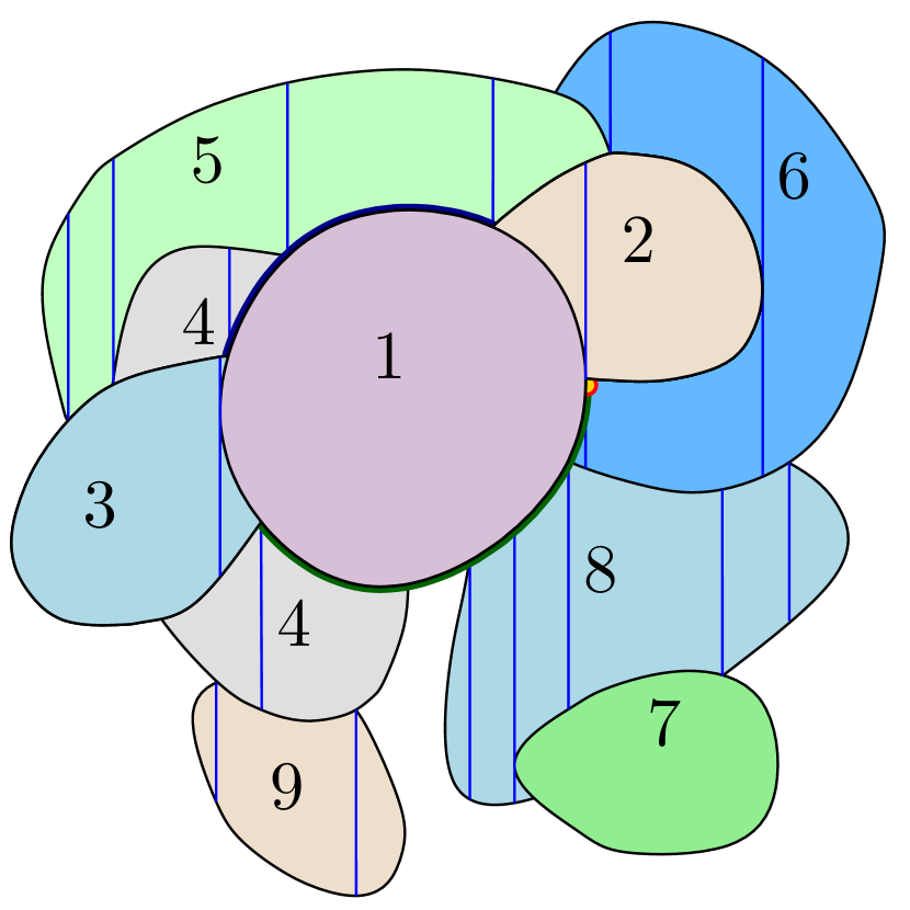
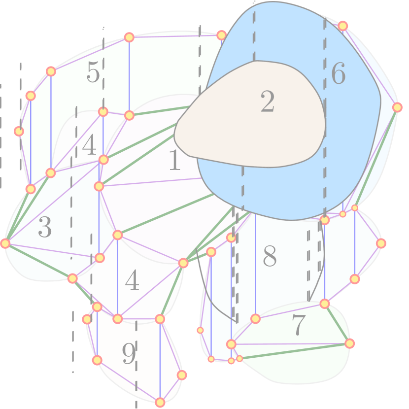
(1) (2) (3) (4) (1’) (2’) (3’) (4’) (8) (7) (6) (5) (8’) (7’) (6’) (5’) (9) (9’) (9”)

Figure 2.2: A step-by-step illustration of the decomposition ${\cal T}$ into pseudo-trapezoids and of the polygonalization of the union. See Section 2.2.4. An animation of this figure is available online at http://sarielhp.org/blog/?p=8920; see also Figure 4.2.

This allows us to order the members of ${\cal D}$ as $D_{1},\ldots,D_{m}$, so that the following property holds. Set ${\cal D}_{i}:=\{D_{1},\ldots,D_{i}\}$, for $i=1,\ldots,m$. Then $D_{i}$ contains at most $c$ intersection points at depths $0$ and $1$ of ${\cal A}({\cal D}_{i})$. Equivalently, for each $i$, the boundary of $D_{i}^{0}:=D_{i}\setminus{\cal U}({\cal D}_{i-1})$ contains at most $c$ intersection points.

To prepare for the algorithmic implementation of the construction in this proof, which will be presented later, we note that this ordering is not easy to obtain efficiently in a deterministic manner. Nevertheless, a random insertion order (almost) satisfies the above property: As we will show, the expected sum of the complexities of the regions $D_{i}^{0}$, for a random insertion order, is $O(m)$. See later for more details.

We thus have ${\cal U}({\cal D}_{j})=\bigcup_{i\leq j}D_{i}^{0}$ (as an openly disjoint union), for each $j$; for the convenience of presentation (and for the algorithm to follow), we interpret this ordering as an incremental process, where the pseudo-disks of ${\cal D}$ are inserted, one after the other, in the order $D_{1},\ldots,D_{m}$, and we maintain the partial unions ${\cal U}({\cal D}_{j})$, after each insertion, by the formula ${\cal U}({\cal D}_{j})={\cal U}({\cal D}_{j-1})\cup D_{j}^{0}$.

2.2.2. Decomposing the union into vertical trapezoids.

Since the boundary of $D_{i}^{0}=D_{i}\setminus{\cal U}({\cal D}_{i-1})$ contains at most $c$ intersection points, we can decompose $D_{i}^{0}$ into $O(1)$ vertical pseudo-trapezoids, using the standard vertical decomposition technique; see, e.g., [SA95]. Let ${\cal T}_{j}$ be the collection of pseudo-trapezoids in the decomposition of ${\cal U}({\cal D}_{j})$, collected from the decompositions of the regions $D_{i}^{0}$, for $i=1,\ldots,j$, and let $V_{j}$ be the set of vertices of these pseudo-trapezoids, each of which is either an intersection point (more precisely, a boundary intersection or an $x$-extreme point) of ${\cal A}({\cal D}_{j})$, or an intersection between some $\partial{\cal D}_{i}$ and a vertical segment erected from an intersection point of ${\cal A}({\cal D}_{j})$.

Each of the pseudo-trapezoids in ${\cal T}_{j}$ is bounded by (at most) two vertical segments, a portion of the boundary of a single pseudo-disk as its top edge, and a portion of the boundary of (another) single pseudo-disk as its bottom edge; see Figure 2.2. We have $D_{1}^{0}=D_{1}$, which we regard as a single pseudo-trapezoid, in which the vertical sides degenerate to the leftmost and rightmost points of $\partial D_{1}$; see Figure 2.2(1). Note that in the vertical decomposition of $D_{i}^{0}$ we split it by vertical segments through the intersection points on its boundary, but not through vertices of $V_{i-1}$ on $\partial D_{i}^{0}$ which are not intersection points of ${\cal A}({\cal D})$. (Informally, these vertices are “internal” to ${\cal U}({\cal D}_{i-1})$, and are not “visible” from the outside.) See, e.g., Figure 2.2(4). The set $V_{i}$ is obtained by adding to $V_{i-1}$ the vertices of the pseudo-trapezoids in the decomposition of $D_{i}^{0}$.

If $D_{i}^{0}$ is bounded then each pseudo-trapezoid $\tau$ in its decomposition has a top boundary and a bottom boundary, but one or both of the vertical sides may be missing (see, e.g., Figure 2.2(1) for the single pseudo-trapezoid $D_{1}^{0}=D_{1}$ and Figure 2.2(3) for the left pseudo-trapezoid of $3$). From the point of view of $\tau$, each of the top and bottom boundaries of $\tau$ may be either convex (if it is a subarc of $\partial D_{i}$ on $\partial D_{i}^{0}$), or concave (if it is part of the boundary of some previously inserted pseudo-disk); If $D_{i}^{0}$ is not bounded then some of the vertical pseudo-trapezoids covering $D_{i}^{0}$ will also be unbounded and missing some of their boundaries. Note that $D_{i}^{0}$ is not necessarily connected; in case it is not connected we separately decompose each of its connected components into vertical pseudo-trapezoids in the above manner; see Figure 2.2(4).

At the end of the incremental process, after inserting all the $m$ pseudo-disks in ${\cal D}$, the pseudo-trapezoids in ${\cal T}:={\cal T}_{m}$ cover ${\cal U}({\cal D})$, which may or may not be the entire plane, and they are pairwise openly disjoint. By construction, each pseudo-trapezoid in ${\cal T}$ is contained in a single pseudo-disk of ${\cal D}$. Moreover, since the complexity of each $D_{i}^{0}$ is $O(1)$, the total number of pseudo-trapezoids in ${\cal T}$ is $O(m)$. So ${\cal T}$ possesses some of the properties that we want, but it is not a triangulation.

2.2.3. Polygonalizing the pseudo-trapezoids.

To get a triangulation, we associate a polygonal vertical pseudo-trapezoid $\tau^{*}$ with each pseudo-trapezoid $\tau\in{\cal T}$. We obtain $\tau^{*}$ from $\tau$ by replacing the bottom boundary $\tau_{b}$ and the top boundary $\tau_{t}$ of $\tau$ by respective polygonal chains $\tau_{b}^{*}$ and $\tau_{t}^{*}$, that are defined as follows. Let $D_{i}$ be the pseudo-disk during whose insertion $\tau$ was created; in particular, $\tau\subseteq D_{i}^{0}$. Let $u$ and $v$ denote the endpoints of $\tau_{b}$. Consider the region $R_{\tau_{b}}$ between $\tau_{b}$ and the straight segment $uv$; clearly, by the convexity of $D_{i}$, $R_{\tau_{b}}$ is fully contained in $D_{i}$. See figure on the right.

If $R_{\tau_{b}}$ contains no vertices of $V_{i}$, other than $u$ and $v$ (this will always be the case when $R_{\tau_{b}}\subseteq\tau$), we replace $\tau_{b}$ by $\tau_{b}^{*}=uv$. Otherwise, we replace $\tau_{b}$ by the chain $\tau_{b}^{*}$ of edges of the convex hull of $V_{i}\cap R_{\tau_{b}}$, other than the edge $uv$. We define $\tau_{t}^{*}$ analogously, and take $\tau^{*}$ to be the polygonal vertical pseudo-trapezoid that has the same vertical edges as $\tau$, and its top (resp., bottom) part is $\tau_{t}^{*}$ (resp., $\tau_{b}^{*}$). See figure on the right.

Note that, by construction, $\tau_{b}^{*}$ is a convex polygonal chain. From the point of view of $\tau$, it is convex (resp., concave) if and only if $\tau_{b}$ is convex (resp., concave). (These statements become somewhat redundant when $\tau_{b}^{*}$ is the straight segnment $uv$.) An analogous property holds for $\tau_{t}^{*}$ and $\tau_{t}$. We denote the crescent-like region bounded by $\tau_{b}$ and $\tau_{b}^{*}$ by $\overline{R}_{\tau_{b}}$; $\overline{R}_{\tau_{t}}$ is defined analogously. (Formally, $\overline{R}_{\tau_{b}}=R_{\tau_{b}}\setminus CH(V_{i}\cap R_{\tau_{b}})$ and $\overline{R}_{\tau_{t}}=R_{\tau_{t}}\setminus CH(V_{i}\cap R_{\tau_{t}})$.) Let ${\cal T}_{i}^{*}$ be the set of polygonal vertical pseudo-trapezoids associated in this manner with the pseudo-trapezoids in ${\cal T}_{i}$.

Note that $R_{\tau_{b}}$ and $R_{\tau_{t}}$ need not be disjoint, as illustrated in the figure on the right. Nevertheless, $\tau_{b}^{*}$ and $\tau_{t}^{*}$ cannot cross one another, as follows from Invariant (I2) that we establish below (in Lemma 2.2). This implies that $\tau^{*}$ is well defined. If $\tau_{b}^{*}$ and $\tau_{t}^{*}$ are not disjoint then they may only be pinched together at common vertices, or overlap in a single common connected portion (in the extreme case they may be identical).

This pinching or overlap, if it occurs, causes the interior of $\tau^{*}$ to be disconnected (into at most two pieces, as depicted in the figure to the right; it may also be empty, as is the case for $D_{1}^{0}$, illustrated in Figure 2.2(1)).

2.2.4. Filling the cavities.

The insertion of $D_{i}$ may in general split some arcs of $\partial{\cal U}({\cal D}_{i-1})$ into subarcs, whose new endpoints are either points of contact between $\partial D_{i}$ and $\partial{\cal U}({\cal D}_{i-1})$, or endpoints of vertical segments erected from other vertices of $D_{i}^{0}$. This can be seen all over Figure 2.2. For example, see the subdivision of the top arc of $D_{7}$ caused by the insertion of $D_{8}$ in Figure 2.2(8’). Some of these subarcs are boundaries of the new pseudo-trapezoids of $D_{i}^{0}$ and thus do not belong to $\partial{\cal U}({\cal D}_{i})$, and some remain subarcs of $\partial{\cal U}({\cal D}_{i})$. We refer to subarcs of the former kind as hidden, and to those of the latter kind as exposed. Note that, among the subarcs into which an arc of $\partial{\cal U}({\cal D}_{i-1})$ is split, only the leftmost and rightmost extreme subarcs can be exposed (this follows from the pseudo-disk property of the objects of ${\cal D}$).

We take each new exposed arc $\gamma$, with endpoints $u,v$, and apply to it the same polygonalization that we applied above to $\tau_{b}$ and $\tau_{t}$. That is, we take the region $R_{\gamma}$ enclosed between $\gamma$ and the segment $uv$, and define $\gamma^{*}$ to be either $uv$, if $R_{\gamma}$ does not contain any vertex of $V_{i}$, or else the boundary of $\mathrm{CH}\left({R_{\gamma}\cap V_{i}}\right)$, except for $uv$. We note that $\gamma^{*}$ is a convex polygonal chain that shares its endpoints with $\gamma$, and denote the region enclosed between $\gamma$ and $\gamma^{*}$ as $\overline{R}_{\gamma}$.

Let $E_{i}$ denote the collection of all straight edges in the polygonal boundaries of the pseudo-trapezoids in ${\cal T}_{i}^{*}$ and in the polygonal chains $\gamma^{*}$ corresponding to new exposed subarcs $\gamma$ of $\partial{\cal U}({\cal D}_{j-1})$, $1\leq j\leq i$, which were created and polygonalized when adding the corresponding pseudo-disk $D_{j}$. See figure on the right.

2.2.5. Putting it all together

When the pseudo-disks cover the plane.

When the polygonalization process terminates, there are no more regions $\overline{R}_{\gamma}$, for boundary arcs $\gamma$ of the union (because there is no boundary), so we are left with a straight-edge planar map $M$ with $E_{m}$ as its set of edges. (Invariant (I1) in Lemma 2.2 below asserts that the edges in $E_{m}$ do not cross each other.) By Euler’s formula, the complexity of $M$ is $O(m)$. We then triangulate each face of $M$, and, as the analysis in the next subsection will show, obtain the desired triangulation.

The general case.

In general, the construction decomposes the union into (pairwise openly disjoint) triangles and crescent regions. To complete the construction, we decompose each crescent region into triangles and caps. A crescent region with $t\geq 2$ vertices on its concave boundary can be decomposed into $t-2$ triangles and at most $t-1$ caps. The case $t=2$ is vacuous, as the crescent is then a cap, so assume that $t\geq 3$. To get such a decomposition, take an extreme edge of the concave polygonal chain, and extend it till it intersects the convex boundary of the crescent, at some point $w$, thereby chopping off a cap from the crescent. We then create the triangles that $w$ spans with all the concave edges that it sees, and then recurse on the remaining crescent; see figure on the right. It is easily seen that this results in $t-2$ triangles and at most $t-1$ caps, as claimed. After this fix-up, we get a decomposition of the union into triangles and caps. Here too, by Euler’s formula, the complexity of $M$ is $O(m)$.

2.3 Analysis

The correctness of the construction is established in the following lemma.

Lemma 2.2.

The pseudo-trapezoids in ${\cal T}_{i}^{*}$ and the edges of $E_{i}$ satisfy the following invariants:

1. The segments in $E_{i}$ do not cross one another.

2. Each subarc $\gamma$ of $\partial{\cal U}({\cal D}_{i})$ with endpoints $u$ and $v$ has an associated convex polygonal arc $\gamma^{*}\subseteq E_{i}$ between $u$ and $v$. The chains $\gamma^{*}$ are pairwise openly disjoint, and their union forms the boundary of a polygonal region ${\cal U}_{i}^{*}\subseteq{\cal U}({\cal D}_{i})$.

3. The pseudo-trapezoids in ${\cal T}_{i}^{*}$ are pairwise openly disjoint, and each of them is fully contained in some pseudo-disk of ${\cal D}_{i}$.

4. ${\cal U}({\cal D}_{i})\setminus\underset{\tau^{*}\in{\cal T}_{i}^{*}}{\bigcup}\tau^{*}$ consists of a collection of pairwise openly disjoint holes. Each hole is a region between two $x$-monotone convex chains or between two $x$-monotone concave chains, with common endpoints, where either both chains are polygonal, or one is polygonal and the other is a portion of the boundary of a single pseudo-disk that lies on $\partial{\cal U}({\cal D}_{i})$. (Each of the latter holes is a crescent-like region of the form $\overline{R}_{\tau_{b}}$, $\overline{R}_{\tau_{t}}$, for some trapezoid $\tau$, or $\overline{R}_{\gamma}$, for some exposed arc $\gamma$, as defined above.) The union of the holes of the latter kind (crescents) is ${\cal U}({\cal D}_{i})\setminus{\cal U}_{i}^{*}$. Each hole, of either kind, is fully contained in some pseudo-disk $D_{j}$, $j\leq i$.

We refer to holes of the former (resp., latter) kind in (I4) of the lemma as internal polygonal holes (resp., external half-polygonal holes).

Proof:

We prove that these invariants hold by induction on $i$. The invariants clearly hold for ${\cal T}_{1}^{*}$ and $E_{1}$ after starting the process with $D_{1}^{0}=D_{1}$. Concretely, ${\cal T}_{1}^{*}$ consists of the single degenerate pseudo-trapezoid $uv$, where $u$ and $v$ are the leftmost and rightmost points of ${\cal D}_{1}$, respectively, and $E_{1}=\{uv\}$. The (external half-polygonal) holes are the portions of $D_{1}$ lying above and below $uv$. It is obvious that (I1)–(I4) hold in this case.

Suppose the invariants hold for ${\cal T}_{i-1}^{*}$ and $E_{i-1}$. We first prove (I1) for $E_{i}$. By construction, the new edges in $E_{i}\setminus E_{i-1}$ form a collection of convex or concave polygonal chains, where each chain $\gamma^{*}$ starts and ends at vertices $u,v$ of either $\partial D_{i}^{0}$ or $\partial{\cal U}({\cal D}_{i-1})$. Moreover, by construction, $u$ and $v$ are connected to one another by a single arc $\gamma$ of the respective boundary $\partial D_{i}^{0}$ or $\partial{\cal U}({\cal D}_{i-1})$ ($\gamma$ is either an exposed or a hidden subarc of $\partial{\cal U}({\cal D}_{i-1})$, or a subarc of $\partial D_{i}$ along $\partial D_{i}^{0}$), and the region $\overline{R}_{\gamma}$ between $\gamma$ and $\gamma^{*}$ does not contain any vertex of $V_{i}$ in its interior.

Clearly, the edges in a single chain $\gamma^{*}$ do not cross one another. Suppose to the contrary that an edge $e$ of some (new) chain $\gamma^{*}$ is crossed by an edge $e^{\prime}$ of some other (new or old) chain. Then either $e^{\prime}$ has an endpoint inside $\overline{R}_{\gamma}$, contradicting the construction, or $e^{\prime}$ crosses $\gamma$ too, to exit from $\overline{R}_{\gamma}$, which again is impossible by construction, since no edge crosses $\partial D_{i}^{0}$ or $\partial{\cal U}({\cal D}_{i-1})$. This establishes (I1).

(I2) follows easily from the construction and from the preceding discussion. Note that, for each polygonal chain $\gamma^{*}$, each of its endpoints is also an endpoint of exactly one neighboring arc $\hat{\gamma}^{*}$, so the union of these arcs consists of closed polygonal cycles, which bound some polygonal region, which we call ${\cal U}_{i}^{*}$, as claimed.

By construction, the vertical boundaries of the new polygonal pseudo-trapezoids of $D_{i}^{0}$ are contained in $D_{i}^{0}$ and do not cross any boundaries of other polygonal pseudo-trapezoids. This, together with (I1), imply that the new pseudo-trapezoids are pairwise openly disjoint, and are also openly disjoint from the polygonal pseudo-trapezoids in ${\cal T}_{i-1}^{*}$. It is also clear from the construction that each new pseudo-trapezoid $\sigma^{*}\in{\cal T}_{i}^{*}\setminus{\cal T}_{i-1}^{*}$ is contained in $D_{i}$. So (I3) follows.

Finally consider (I4). Each new hole that is created when adding $D_{i}^{0}$ is of one of the following kinds:

(a) The hole is a region of the form $\overline{R}_{\tau_{b}}$ or $\overline{R}_{\tau_{t}}$, for some $\tau\in{\cal T}_{i}\setminus{\cal T}_{i-1}$, such that $\overline{R}_{\tau_{b}}$ or $\overline{R}_{\tau_{t}}$ is contained in $\tau$ (if it lies outside $\tau$, it becomes part of $\tau^{*}$). Such a hole is contained in $D_{i}$, and is bounded by two concave or two convex chains, one of which, call it $\zeta^{*}$, is polygonal, and the other, $\zeta$, is part of $\partial D_{i}^{0}$. Moreover, $\zeta^{*}$, if different from the chord $e$ connecting the endpoints of $\zeta$, passes through inner vertices of $\partial{\cal U}({\cal D}_{i-1})$ that “stick into” the corresponding portion $R_{\tau_{b}}$ or $R_{\tau_{t}}$ of $\tau$; see figure on the right.

(b) The hole is a region of the form $\overline{R}_{\gamma}$, for an exposed subarc $\gamma$ of an arc of $\partial{\cal U}({\cal D}_{i-1})$, that got delimited by a new vertex (an endpoint of some arc of $\partial D_{i}$). These holes are similar to those of type (a).

(c) The hole was part of a hole of type (a) or (b) in ${\cal U}({\cal D}_{i-1})$, bounded by an arc $\gamma$ of $\partial{\cal U}({\cal D}_{i-1})$ and its associated polygonal chain $\gamma^{*}$, so that $\gamma$ has been split into several subarcs (some hidden and some exposed) when adding $D_{i}$. For each of these subarcs $\zeta$, we construct an associated polygonal chain $\zeta^{*}$, either as a top or bottom side of some polygonal pseudo-trapezoid $\tau^{*}$ (constructed from a pseudo-trapezoid $\tau$ that has $\zeta$ as its top or bottom side), or as the polygonalization of an exposed subarc. The concatenation of the chains $\zeta^{*}$ results in a convex polygonal chain that is contained in $\overline{R}_{\gamma}$ and connects the endpoints of $\gamma$. The region enclosed between $\gamma^{*}$ and $\zeta^{*}$ is an internal polygonal hole. Again, holes of type (c) can be seen all over Figure 2.2; for example, see the top part of $D_{1}$ in Figure 2.2(2’).

Holes of type (a) and (b) are boundary half-polygonal holes, whereas holes of type (c) are internal polygonal holes. Using the induction hypothesis that (I4) holds for ${\cal U}({\cal D}_{i-1})$, we get that the union of the new holes of type (a) and (b), together with the old holes of type (a) and (b) corresponding to subarcs of $\partial{\cal U}({\cal D}_{i})\cap\partial{\cal U}({\cal D}_{i-1})$, is ${\cal U}({\cal D}_{i})\setminus{\cal U}_{i}^{*}$. This completes the proofs of (I1)–(I4).  

Theorem 2.3.

(a) Let ${\cal D}$ be a collection of $m\geq 3$ planar convex pseudo-disks, whose union covers the plane. Then there exists a set $V$ of $O(m)$ points and a triangulation $T$ of $V$ that covers the plane, such that each triangle $\Delta\in T$ is fully contained in some member of ${\cal D}$.

(b) If ${\cal U}({\cal D})$ is not the entire plane, it can be partitioned into $O(m)$ pairwise openly disjoint triangles and caps, such that each triangle and cap is fully contained in some member of ${\cal D}$.

Proof:

Since the number of vertices of $M$ is $O(m)$, Euler’s formula implies that $|E_{m}|=O(m)$ too. It is easily seen from the construction and from the invariants of Lemma 2.2, that each face of $M$ is fully contained in some original pseudo-disk, so the same holds for each triangle. This establishes (a). Part (b) follows in a similar manner from the construction.  

2.4 Efficient construction of the triangulation

With some care, the proof of Theorem 2.3 can be turned into an efficient algorithm for constructing the required triangulation. This is a major advantage of the new proof over the older one. The algorithm is composed of building blocks that are variants of well-known tools, so we only give a somewhat sketchy description thereof

2.4.1. Construction of the original pseudo-trapezoids.

(A similar approach is mentioned in Matoušek et al. [MMP⁺91].) The construction proceeds by inserting the pseudo-disks of ${\cal D}$ in a random order, which, for simplicity, we denote as $D_{1},\ldots,D_{m}$. (Unlike the deterministic construction given above, here we do not guarantee that each $D_{i}^{0}$ has constant complexity. Nevertheless, as argued below, the random nature of the insertion order guarantees that this property holds on average.) As before, we put ${\cal D}_{i}=\{D_{1},\ldots,D_{i}\}$ for each $i$, and we maintain ${\cal U}({\cal D}_{i})$ after each insertion of a pseudo-disk. To do so efficiently, we maintain a vertical decomposition $K_{i}$ of the complement ${\cal U}_{i}^{c}$ of the union ${\cal U}({\cal D}_{i})$ into vertical pseudo-trapezoids (as depicted in the figure on the right), and maintain, for each $\tau\in K_{i}$, a conflict list, consisting of all the pseudo-disks $D_{j}$ that have not yet been inserted (i.e., with $j>i$), and that intersect $\tau$.

(Micha says: Fig. pdcompl needs fixing.) Since the number of pseudo-trapezoids in the decomposition of the complement of the union of any $k$ pseudo-disks (as depicted in the figure on the right) is $O(k)$ (an easy consequence of the linear bound on the union complexity [KLPS86]), a simple application of the Clarkson-Shor technique (similar to those used to analyze many other randomized incremental algorithms) shows that the expected overall number of these “complementary” pseudo-trapezoids that arise during the construction is $O(m)$, and that the expected overall size of their conflict lists is $O(m\log m)$.

When we insert a pseudo-disk $D_{i}$, we retrieve all the pseudo-trapezoids of $K_{i-1}$ that intersect $D_{i}$. The union $\bigcup_{\tau\in K_{i-1}}(D_{i}\cap\tau)$ is precisely $D_{i}^{0}$. For each $\tau\in K_{i-1}$, the intersection $D_{i}\cap\tau$ (if nonempty) decomposes $\tau$ into $O(1)$ sub-trapezoids (this follows from the property that each of the four sides of $\tau$ crosses $\partial D_{i}$ at most twice), some of which lie inside $D_{i}$ (and, as just noted, form $D_{i}^{0}$), and some lie outside $D_{i}$, and form part of the new complement of the union ${\cal U}_{i}^{c}$.

Typically, the new pseudo-trapezoidal pieces are not necessarily real pseudo-trapezoids, as they may contain one or two “fake” vertical sides, because the feature that created such a side got “chopped off” by the insertion of $D_{i}$, and is no longer on the pseudo-trapezoid boundary. In this case, we “glue” these pieces together, across common fake vertical sides, to form the new real pseudo-trapezoids. We do it both for pseudo-trapezoids that are interior to $D_{i}$, and for those that are exterior. (This gluing step is a standard theme in randomized incremental constructions; see, e.g., [Sei91].) This will produce (a) the desired vertical decomposition of $D_{i}^{0}$, and (b) the vertical decomposition $K_{i}$ of the new union complement ${\cal U}_{i}^{c}$. The conflict lists of the new exterior pseudo-trapezoids (interior ones do not require conflict lists) are assembled from the conflict lists of the pseudo-trapezoids that have been destroyed during the insertion of $D_{i}$, again, in a fully standard manner.

To recap, this procedure constructs the vertical decompositions of all the regions $D_{i}^{0}$, so that the overall expected number of these pseudo-trapezoids is $O(m)$, and the total expected cost of the construction (dominated by the cost of handling the conflict lists) is $O(m\log m)$.

2.4.2. Construction of the polygonal chains and the triangulation.

By (I2) of Lemma 2.2, before $D_{i}$ was inserted, each arc $\gamma$ of $\partial{\cal U}({\cal D}_{i-1})$ has an associated convex polygonal arc $\gamma^{*}$ with the same endpoints. The union of the arcs $\gamma^{*}$ forms a (possibly disconnected) polygonal curve within ${\cal U}({\cal D}_{i-1})$, which partitions it into two subsets, the (polygonal) interior, ${\cal U}_{i-1}^{*}$, which is disjoint from $\partial{\cal U}({\cal D}_{i-1})$ (except at the endpoints of the arcs $\gamma^{*}$), and the (half-polygonal) exterior, which is simply the (pairwise openly disjoint) union of the corresponding regions $\overline{R}_{\gamma}$.

To construct the triangulation, we maintain, for each polygonal chain $\gamma^{*}$ of the boundary between the interior and the exterior, a list of its segments, sorted in left-to-right order of their $x$-projections, in a separate binary search tree (since the leftmost and rightmost points of each pseudo-disk are vertices in the construction, each chain $\gamma^{*}$ is indeed $x$-monotone). We also maintain a triangulation of the interior. When we add $D_{i}$ we update the lists representing the arcs $\gamma$ and extend the triangulation of the interior to cover the “newly annexed” interior, as follows.

When $D_{i}$ is inserted, some of the arcs $\gamma$ of $\partial{\cal U}({\cal D}_{i-1})$ are split into several subarcs. At most two of these arcs still appear on $\partial{\cal U}({\cal D}_{i})$, and each of them is an extreme subarc of $\gamma$ (we call them, as above, exposed arcs). All the others are now contained in $D_{i}$ (we call them hidden). Each endpoint of any new subarc is either an intersection point of $\partial D_{i}$ with $\partial{\cal U}({\cal D}_{i-1})$, or an endpoint of a vertical segment erected from some other vertex of $D_{i}^{0}$. (This also includes the case where an arc of $\partial{\cal U}({\cal D}_{i-1})$ is fully “swallowed” by $D_{i}$ and becomes hidden in its entirety.) In addition, $\partial{\cal U}({\cal D}_{i})$ contains fresh arcs, which are subarcs of $\partial D_{i}$ along $\partial D_{i}^{0}$. The fresh subarcs and the hidden subarcs form the top and bottom sides of the new pseudo-trapezoids in the decomposition of $D_{i}^{0}$ (where each top or bottom side may be either fresh or hidden). To obtain the top or bottom sides of some new pseudo-trapezoids we may have to concatenate several previously exposed subarcs of $\partial{\cal U}({\cal D}_{i-1})$. These subarcs are connected at “inner” vertices of $\partial{\cal U}({\cal D}_{i-1})$ which are not intersection points of the arrangement but intersections of vertical sides of pseudo-trapezoids which we already generated within ${\cal U}({\cal D}_{i-1})$.)

The algorithm needs to construct, for each new exposed, hidden, and fresh arc $\gamma$, its associated polygonal curve $\gamma^{*}$. It does so in two stages, first handling exposed and hidden arcs, and then the fresh ones. Let $\gamma$ be an exposed or hidden subarc, let $\delta$ denote the arc of $\partial{\cal U}({\cal D}_{i-1})$, or the concatenation of several such arcs, containing $\gamma$, and let $\delta^{*}$ be its associated polygonal chain, or, in case of concatenation, the concatenation of the corresponding polygonal chains. As already noted, since the $x$-extreme points of each pseudo-disk boundary are vertices in the construction, $\delta$ and $\delta^{*}$ are both $x$-monotone.

If $\gamma=\delta$, we do nothing, as $\gamma^{*}=\delta^{*}$. Otherwise, let $u$ and $v$ be the respective left and right endpoints of $\gamma$. If $uv$ does not intersect $\delta^{*}$ then $\gamma^{*}$ is just the segment $uv$. Otherwise, $\gamma^{*}$ is obtained from a portion of $\delta^{*}$, delimited on the left by the point $u^{\prime}$ of contact of the right tangent from $u$ to $\delta^{*}$, and on the right by the point $v^{\prime}$ of contact of the left tangent from $v$ to $\delta^{*}$, to which we append the segments $uu^{\prime}$ on the left and $v^{\prime}v$ on the right. See Figure 2.4.2 for an illustration.

Note that the old arc $\delta$ may contain several new exposed or hidden arcs $\gamma$, so we apply the above procedure to each such arc $\gamma$. After doing this, the endpoints of $\delta$ (and of $\delta^{*}$) are now connected by a new convex polygonal chain $\hat{\delta}^{*}$, which visits each of the new vertices along $\delta$ (the endpoints of the new arcs $\gamma$) and lies in between $\delta$ and $\delta^{*}$. The region between $\hat{\delta}^{*}$ and $\delta^{*}$ is a new interior polygonal hole, and we triangulate it, e.g., into vertical trapezoids, by a straightforward left-to-right scan.

Recall that some arcs $\tau_{b}$ and $\tau_{t}$ of new trapezoids $\tau$ may be concatenations of several hidden subarcs $\gamma_{i}$ (connected at inner vertices which are not vertices of new trapezoids, as explained above). For each such arc, say $\tau_{b}$, we obtain $\tau_{b}^{*}$ by concatenating the polygonal chains $\gamma_{i}^{*}$ in $x$-monotone order.

We next handle the fresh arcs. Each such arc is the top or bottom side of some new pseudo-trapezoid $\tau$, say it is the bottom side $\tau_{b}$. If $\tau_{t}$ is also fresh, then $\tau$ is a convex pseudo-trapezoid, and we replace each of $\tau_{b}$, $\tau_{t}$ by the straight segment connecting its endpoints. If $\tau_{t}$ is hidden, we take its associated chain $\tau_{t}^{*}$, which we have constructed in the preceding stage, and form $\tau_{b}^{*}$ from it using the same procedure as above: Letting $u$ and $v$ denote the endpoints of $\tau_{b}$, we check whether $uv$ intersects $\tau_{t}^{*}$. If not, $\tau_{b}^{*}$ is the segment $uv$. Otherwise, we compute the tangents from $u$ and $v$ to $\tau_{t}^{*}$, and form $\tau_{b}^{*}$ from the tangent segments and the portion of $\tau_{t}^{*}$ between their contact points. See figure on the right. We triangulate each polygonal pseudo-trapezoid $\tau$ once we have computed $\tau_{b}^{*}$ and $\tau_{t}^{*}$.

2.4.3. Further implementation details.

The actual implementation of the construction of the polygonal chains $\gamma^{*}$ proceeds as follows. Given a new arc $\gamma$, which is a subarc of an old arc $\delta$, we construct $\gamma^{*}$ from $\delta^{*}$ as follows. Let $u$ and $v$ be the endpoints of $\gamma$. We (binary) search the list of edges of $\delta^{*}$ for the edge $e_{u}$ whose $x$-projection contains the $x$-projection of $u$ and for the edge $e_{v}$ whose $x$-projection contains the $x$-projection of $v$. We then walk along the list representing $\delta^{*}$ from $e_{u}$ towards $e_{v}$ until we find the point $u^{\prime}$ of contact of the right tangent from $u$ to $\delta^{*}$. We perform a similar search from $e_{v}$ towards $e_{u}$ to find $v^{\prime}$. (If we have traversed the entire portion of $\delta^{*}$ between $e_{u}$ and $e_{v}$ without encountering a tangent, we conclude that $uv$ does not intersect $\delta^{*}$, and set $\gamma^{*}:=uv$.) We extract the sublist between $u^{\prime}$ and $v^{\prime}$ from $\delta^{*}$ by splitting $\delta^{*}$ at $u^{\prime}$ and $v^{\prime}$ and we insert the segments $uu^{\prime}$ and $vv^{\prime}$ at the endpoints of this sublist to obtain $\gamma^{*}$. We create the polygonalization of fresh arcs from their hidden counterparts in an analogous manner. Note that we destroy the representation of $\delta^{*}$ to produce the representation of $\gamma^{*}$. So in case the arc $\delta$ is split into several new subarcs, $\gamma_{i}$, some care has to be taken to maintain a representation of the remaining part of $\delta^{*}$ after producing each $\gamma_{j}^{*}$, from which we can produce the representation of the remaining subarcs $\gamma_{i}$.

For the analysis, we note that to produce $\gamma^{*}$ we perform two binary searches to find $e_{u}$ and $e_{v}$, each of which takes $O(\log m)$ time, and then perform linear scans to locate $u^{\prime}$ and $v^{\prime}$. Each edge $e$ traversed by these linear scans (except for $O(1)$ edges) drops off the boundary of the interior so we can charge this step to $e$ and the total number of such charges is linear in the size of the triangulation.

2.5 The result

The computation model.

In the preceding description, we implicitly assume a convenient model of computation, in which each primitive geometric operation that is needed by the algorithm, and that involves only a constant number of pseudo-disks (e.g., deciding whether two pseudo-disks or certain subarcs thereof intersect, computing these intersection points, and sorting them along a pseudo-disk boundary) takes constant time. In our application, described in the next section, the pseudo-disks are convex polygons, each having $O(k)$ edges. In this case, each primitive operation can be implemented in $O(\log k)$ time in the standard (say, real RAM) model, so the running time should be multiplied by this factor.

The preceding analysis implies the following theorem.

Theorem 2.4.

We can construct a triangulation of the union of $m$ pseudo-disks covering the plane, with $O(m)$ triangles, such that each triangle is contained in a single pseudo-disk, in $O(m\log m)$ randomized expected time, in a suitable model of computation where every primitive operation takes $O(1)$ time. If the union does not cover the plane, it can be decomposed into $O(m)$ triangles and caps, with similar properties and at the same asymptotic cost.

Corollary 2.5.

Given $m$ convex polygons that are pseudo-disks, that cover that plane, each with at most $k$ edges, one can compute a confined triangulation of the plane, in $O(m\log m\log k)$ expected time. A statement analogous to the second part of Theorem 2.4 holds in this case too.

2.6 Extension to general convex shapes

Theorem 2.4 uses only peripherally the property that the input shapes are pseudo-disks, and a simple modification (of the analysis, not of the construction itself) allows us to extend it to general convex shapes. Specifically, let ${\cal D}$ be a collection of $m$ simply-shaped convex regions in the plane, such that the union complexity of any $i$ of them is at most $u(i)$, where the complexity is measured, as before, by the number of boundary intersection points on the union boundary, and where $u(\cdot)$ is a monotone increasing function satisfying $u(i)=\Omega(i)$. We assume that the regions in ${\cal D}$ are simple enough so that the boundaries of any pair of them intersect only a constant number of times, and so that each primitive operation on them can be performed in reasonable time (which we take to be $O(1)$ in the statement below). The interesting cases are those in which $u(i)$ is small (that is, near-linear). They include, e.g., the case of fat triangles, or a low-density collection of convex regions; see [AdBES14] and references therein.

Deploying the algorithm of Theorem 2.4 results in the desired confined triangulation of ${\cal U}({\cal D})$. Extending the analysis to this general setup (and omitting the straightforward technical details), we obtain the following theorem.

Theorem 2.6.

Let ${\cal D}$ be a collection of $n$ convex shapes in the plane, such that the union complexity of any $i$ of them is at most $u(i)$, where $u(i)$ is a monotone increasing function with $u(i)=\Omega(i)$. Then one can compute, in $O(u(m)\log m)$ expected time, a confined triangulation of ${\cal U}({\cal D})$ with $O(u(m))$ triangles and caps (or just triangles if the union covers the entire plane), under the assumption that every primitive geometric operation takes $O(1)$ time.

3 Construction of shallow cuttings and approximate levels

We begin by presenting a high-level description of the technique, filling in the technical details in subsequent subsections. The high-level part does not pay too much attention to the efficiency of the construction; this is taken care of later in this section.

3.1 Sketch of the construction

Assume that, for a given parameter $r$, we want to approximate level $k=n/r$ of ${\cal A}(H)$. Note that when $r$ is too close to $n$, that is, when $k$ is a constant, we can simply compute the $k$-level explicitly and use it as its own approximation. The complexity of such a level is $O(n)$, and it can be computed in $O(n\log n)$ time [Cha10, AM95] (better than what is stated in Theorem 3.3 for such a large value of $r$). We therefore assume in the remainder of this section that $r\ll n$.

Put $k_{1}:=(1+c)n/r$ and $k_{2}:=(1+2c)n/r$, for a suitable sufficiently small (but otherwise arbitrary) constant fraction $c$. The analysis of Clarkson and Shor [CS89] implies that the overall complexity of $L_{\leq k_{2}}$ (the first $k_{2}$ levels of ${\cal A}(H)$) is $O(nk^{2})$. This in turn implies that there exists an index $k_{1}\leq\xi\leq k_{2}$ for which the complexity $|L_{\xi}|$ of $L_{\xi}$ is $O(nk^{2}/(cn/r))=O(nk/c)=O(n^{2}/(cr))$. We fix such a level $\xi$, and continue the construction with respect to $L_{\xi}$ (slightly deviating from the originally prescribed value of $k$). However, to simplify the notation for the current part of the analysis, we use $k$ to denote the nearby level $\xi$, and will only later return to the original value of $k$.

The next step is to decompose the $xy$-projection of the $k$-level $L_{k}$ into a small number of connected polygons, from which the approximate level will be constructed. We first review the existing machinery, already mentioned in the introduction, for this step.

Decomposing a level into a small number of polygons.

Let $H$, $k$, and $L_{k}$ be as above. It is convenient to assume that the faces of $L_{k}$ are triangles; this can be achieved by triangulating each face, without affecting the asymptotic complexity of $L_{k}$. In particular, the $k$-level (or, rather, its $xy$-projection) can then be interpreted as a planar, triangulated and biconnected graph (a graph is biconnected, if any pair of vertices are connected by at least two vertex-disjoint paths).

As has been discovered over the years, planar graphs can be efficiently decomposed into smaller pieces that are well behaved. This goes back to the planar separator theorem of Lipton and Tarjan [LT79], Miller’s cycle separator theorem [Mil86], and Frederickson’s divisions [Fre87], and has eventually culminated in the fast $\kappa$-division algorithm of Klein et al. [KMS13]. Specifically, for a (specific drawing of a) planar triangulated and biconnected graph $G$ with $N$ vertices, and for a parameter $\kappa<n$, a $\kappa$-division of $G$ is a decomposition of $G$ into several connected subgraphs $G_{1},\ldots,G_{m}$, such that (i) $m=O(N/\kappa)$; (ii) each $G_{i}$ has at most $\kappa$ vertices; (iii) each $G_{i}$ has at most $\beta\sqrt{\kappa}$ boundary vertices, for some absolute constant $\beta$, namely, vertices that belong to at least one additional subgraph; and (iv) each $G_{i}$ has at most $O(1)$ holes, namely, faces of the induced drawing of $G_{i}$ that are not faces of $G$ (as they contain additional edges and vertices of $G$). Such a division can be computed in $O(N)$ time [KMS13].

The construction, continued.

We set

$$t:=\frac{cn-43.5r}{9\beta r},$$

where $\beta$ is the constant from property (iii) of the $\kappa$-division given above. Notice that since $r\ll n$ we have $t>1$. Let $L^{\prime}_{k}$ be the projection of $L_{k}$ to the $xy$-plane. We turn $L^{\prime}_{k}$ into a triangulated and biconnected planar graph $G^{\prime}_{k}$ by adding a new vertex $v_{\infty}$, replacing each ray $[p,\infty)$ by the edge $(p,v_{\infty})$, and triangulating the newly created faces. We apply the planar subdivision algorithm of [KMS13, Fre87], as just reviewed, and construct a $t^{2}$-division of $G^{\prime}_{k}$. This subdivision produces

$$m:=O(|L_{k}|/t^{2})=O\left(\frac{n^{2}/(cr)}{c^{2}n^{2}/r^{2}}\right)=O(r/c^{3})$$

connected polygons, $P^{\prime}_{1},\ldots,P^{\prime}_{m}$, with pairwise disjoint interiors. Each polygon $P^{\prime}_{i}$ corresponds to a (possibly unbounded) polygon $P_{i}$ of $L^{\prime}_{k}$. The union of $P_{1},\ldots,P_{m}$ covers the entire $xy$-plane, and its edges are projections of (some) edges of $L_{k}$ (including diagonals drawn to triangulate the original faces of $L_{k}$).

By construction, each $P_{i}$ is connected and has at most $\beta t$ edges (and also contains $O(t^{2})$ edges and vertices of the projected $k$-level in its interior). Let $C_{i}$ denote the convex hull of $P_{i}$, for $i=1,\ldots,m$. As we show in Corollary 3.5 in Section 3.3 below, ${\cal C}:=\{C_{1},\ldots,C_{m}\}$ is a collection of $m$ (possibly unbounded) convex pseudo-disks whose union is the entire plane.

We then apply Theorem 2.3 to ${\cal C}$ and obtain a set $S$ of $O(m)$ points in the $xy$-plane, and a triangulation $T$ of $S$, such that each triangle $\Delta\in T$ is fully contained in some hull $C_{i}$ in ${\cal C}$. For a point $p$ in the $xy$-plane, we denote by ${\bf\uparrow}_{k}(p)$ the lifting of $p$ to the $k$-level, i.e., the point on the level that is co-vertical with $p$.

For a bounded triangle $\Delta$, ${\bf\uparrow}_{k}(\Delta)$ is defined as the triangle spanned by the lifted images of the three vertices of $\Delta$; we lift an unbounded triangle $\Delta$ with vertices $p$ and $q$ by lifting $pq$ to ${\bf\uparrow}_{k}(p){\bf\uparrow}_{k}(q)$ as before, and lifting each of its rays, say $[p,\infty)$, to a ray ${\bf\uparrow}([p,\infty))$ emanating from ${\bf\uparrow}_{k}(p)$ in a direction parallel to the plane which is vertically above $[p,\infty)$ at infinity. If the liftings ${\bf\uparrow}([p,\infty))$, and ${\bf\uparrow}([q,\infty))$, and the edge ${\bf\uparrow}_{k}(p){\bf\uparrow}_{k}(q)$ are not on the same plane, we add another ray, say $r$, emanating from $p$ parallel to $[q,\infty)$. We add to $T^{\prime}$ the unbounded triangle spanned by ${\bf\uparrow}([q,\infty))$, ${\bf\uparrow}_{k}(p){\bf\uparrow}_{k}(q)$, and $r$, and the unbounded wedge spanner by $r$ and ${\bf\uparrow}([p,\infty))$. Let $T^{\prime}$ denote the corresponding collection of triangles in $\mathbb{R}^{3}$, given by $T^{\prime}=\{{\bf\uparrow}_{k}(\Delta)\mid\Delta\in T\}$.

Note that the triangles of $T^{\prime}$ are in general not contained in $L_{k}$. However, for each triangle $\Delta^{\prime}\in T^{\prime}$, its vertices lie on $L_{k}$, and, as we show in Lemma 3.8 below, at most $9\beta t+43.5$ planes of $H$ can cross $\Delta^{\prime}$. This implies, returning now to the original value of $k$, that $\Delta^{\prime}$ fully lies between the levels

$$\xi\pm(9\beta t+43.5)=\xi\pm cn/r$$

of ${\cal A}(H)$. In particular, $\Delta^{\prime}$ lies fully above the level

$$\xi-cn/r\geq k_{1}-cn/r=n/r=k,$$

and fully below the level

$$\xi+cn/r\leq k_{2}+cn/r=(1+3c)n/r=(1+3c)k.$$

The lifted triangulation $T^{\prime}$ forms a polyhedral terrain that consists of $O(r/c^{3})$ triangles and is contained between the levels $k=n/r$ and $(1+3c)k$. That is, for a given ${\varepsilon}>0$, choosing $c={\varepsilon}/3$ makes $T^{\prime}$ an ${\varepsilon}$-approximation of $L_{k}$, and we obtain the following result.

Theorem 3.1.

Let $H$ be a set of $n$ non-vertical planes in $\mathbb{R}^{3}$ in general position, and let $r\leq n$, ${\varepsilon}>0$ be given parameters. Then there exists a polyhedral terrain consisting of $O(r/{\varepsilon}^{3})$ triangles, that is fully contained between the levels $n/r$ and $(1+{\varepsilon})n/r$ of ${\cal A}(H)$.

To turn this approximate level into a shallow cutting, replace each $\Delta^{\prime}\in T^{\prime}$ (including each of the unbounded triangles as constructed above) by the semi-unbounded vertical prism $\Delta^{*}$ consisting of all the points that lie vertically below $\Delta^{\prime}$. This yields a collection $\Xi$ of prisms, with pairwise disjoint interiors, whose union covers $L_{\leq n/r}$, so that, for each prism $\tau$ of $\Xi$, we have (a) each vertex of $\tau$ lies at level (at least $k$ and) at most $(1+\frac{2}{3}{\varepsilon})k$, and, as will be established in Lemma 3.8 below, (b) the top triangle of $\tau$ is crossed by at most $\frac{1}{3}{\varepsilon}k$ planes of $H$ (in the preceding analysis, we wrote this bound as $9\beta t+43.5=\frac{cn}{r}$; this is the same value, recalling that ${\varepsilon}=3c$ and $k=n/r$). Hence, as is easily seen, each prism of $\Xi$ is crossed by at most $(1+{\varepsilon})n/r$ planes, so $\Xi$ is the desired shallow cutting. That is, we have the following result.

Theorem 3.2.

Let $H$ be a set of $n$ non-vertical planes in $\mathbb{R}^{3}$ in general position, let $k<n$ and ${\varepsilon}>0$ be given parameters, and put $r=n/k$. Then there exists a $k$-shallow $((1+{\varepsilon})/r)$-cutting of ${\cal A}(H)$, consisting of $O(r/{\varepsilon}^{3})$ vertical prisms (unbounded from below). The top of each prism is a triangle that is fully contained between the levels $k$ and $(1+{\varepsilon})k$ of ${\cal A}(H)$, and these triangles form a polyhedral terrain (we say that such a terrain approximates the $k$-level $L_{k}$ up to a relative error of ${\varepsilon}$).

3.2 Efficient implementation

We next turn our constructive proof into an efficient algorithm, and show:

Theorem 3.3.

Let $H$ be a set of $n$ non-vertical planes in $\mathbb{R}^{3}$ in general position, let $k<n$ and ${\varepsilon}>0$ be given parameters, and put $r=n/k$. One can construct the $k$-shallow $((1+{\varepsilon})/r)$-cutting of ${\cal A}(H)$ given in Theorem 3.2, or, equivalently, the ${\varepsilon}$-approximating terrain of the $k$-level in Theorem 3.1, in $O(n+r{\varepsilon}^{-6}\log^{3}r)$ expected time. Computing the conflict lists of the vertical prisms takes an additional $O(n({\varepsilon}^{-3}+\log\frac{r}{{\varepsilon}}))$ expected time. The algorithm, not including the construction of the conflict lists, computes a correct ${\varepsilon}$-approximating terrain with probability at least $1-1/r^{O(1)}$. If we also compute the conflict lists then we can verify, in $O(n/{\varepsilon}^{3})$ time, that the cutting is indeed correct and thereby make the algorithm always succeed, at the cost of increasing its expected running time by a constant factor.

Proof:

Let $(H,\mathcal{R})$ denote the range space where each range in $\mathcal{R}$ corresponds to some vertical segment or ray $e$, and is equal to the subset of the planes of $H$ that are crossed by $e$. Clearly, $(H,\mathcal{R})$ has finite VC-dimension (see, e.g., [SA95]). We draw a random sample $S$ of ${\displaystyle n^{\prime}=\frac{br}{{\varepsilon}^{2}}\log r}$ planes from $H$, where $b$ is a suitable constant. For $b$ sufficiently large, such a sample is a relative $\left(\frac{1}{r},{\varepsilon}\right)$-approximation for $(H,\mathcal{R})$, with probability $\geq 1-1/r^{O(1)}$; see [HS11] for the definition and properties of relative approximations. This means that each vertical segment or ray that intersects $x\geq n/r$ planes of $H$ intersects between $({1+{\varepsilon}})\frac{n^{\prime}}{n}x$ and $({1-{\varepsilon}})\frac{n^{\prime}}{n}x$ planes of $S$, and each vertical segment or ray that intersects $x<n/r$ planes of $H$ intersects at most $\frac{n^{\prime}}{n}x+{\varepsilon}\frac{n^{\prime}}{r}$ planes of $S$. (This holds, with probability $\geq 1-1/r^{O(1)}$, for all vertical segments and rays.)

The strategy is to use (the smaller) $S$ instead of $H$ in the construction, as summarized in Theorem 3.2, and then argue that a suitable approximate level in ${\cal A}(S)$ is also an approximation to level $k$ in ${\cal A}(H)$ with the desired properties. Set

$$k^{\prime}=\frac{b(1+{\varepsilon})}{{\varepsilon}^{2}}\log r,\quad\text{and}\quad t^{\prime}=\frac{b(1+{\varepsilon})}{{\varepsilon}}\log r={\varepsilon}k^{\prime}.$$

We choose a random index $\xi$ in the range $[k^{\prime},k^{\prime}+t^{\prime}]$, construct the $\xi$-level of ${\cal A}(S)$, and then apply the construction of the proof of Theorem 3.2 to this level, as will be detailed below.

Before doing this, we first show that the $\xi$-level in ${\cal A}(S)$ is a good approximation to level $k$ in ${\cal A}(H)$. Consider a point $p$ on level $k$ of ${\cal A}(H)$. By the property specified above of a relative $\left(\frac{1}{r},{\varepsilon}\right)$-approximation, it follows that the level of $p$ in ${\cal A}(S)$ is at most $(1+{\varepsilon})(n^{\prime}/n)(n/r)=k^{\prime}$. Similarly, let $p$ be a point at level larger than, say, $(1+4{\varepsilon})k$ of ${\cal A}(H)$. Then the level of $p$ in ${\cal A}(S)$ is at least $(1-{\varepsilon})(n^{\prime}/n)(1+4{\varepsilon})(n/r)\geq(1+{\varepsilon})k^{\prime}=k^{\prime}+t^{\prime}$, for ${\varepsilon}\leq 1/2$. Since this holds with probability $\geq 1-1/r^{O(1)}$, for every point $p$, we conclude that the entire $\xi$-level of ${\cal A}(S)$ is between levels $k$ and $(1+4{\varepsilon})k$ of ${\cal A}(H)$, with probability $\geq 1-1/r^{O(1)}$.

We can now apply the machinery in Theorem 3.2. The first step in this analysis is to construct the $\xi$-level in ${\cal A}(S)$. Rather than just constructing that level, we compute all the first $k^{\prime}+t^{\prime}$ levels, using a randomized algorithm of Chan [Cha00], which takes

$$O(n^{\prime}\log n^{\prime}+n^{\prime}(k^{\prime})^{2}) =O\left({\frac{r\log r}{{\varepsilon}^{2}}\left({\log\frac{r}{{\varepsilon}}+\frac{\log^{2}r}{{\varepsilon}^{4}}}\right)}\right)=O\left({r{\varepsilon}^{-6}\log^{3}r}\right)$$

expected time. We can then easily extract the desired (random) level $\xi$. In expectation (over the random choice of $\xi$), the complexity of the $\xi$-level is

$$n_{1}=O\left({n^{\prime}(k^{\prime})^{2}/({\varepsilon}k^{\prime})}\right)=O\left({n^{\prime}k^{\prime}/{\varepsilon}}\right)=O\left(\frac{r}{{\varepsilon}^{5}}\log^{2}r\right),$$

and we assume in what follows that this is indeed the case.

We now continue the implementation of the construction in a straightforward manner. We already have the random $\xi$-level. We project it onto the $xy$-plane, and construct a $(t^{\prime})^{2}$-division of the projection, in $O(n_{1})$ time. It consists of

$$m:=O(n_{1}/(t^{\prime})^{2})=O\left(\frac{n^{\prime}}{{\varepsilon}^{3}k^{\prime}}\right)=O(r/{\varepsilon}^{3})$$

pieces, each with $O(t^{\prime})=O\left(\frac{1}{{\varepsilon}}\log r\right)$ edges. We compute their convex hulls in $O(mt^{\prime})=O(\frac{r}{{\varepsilon}^{4}}\log r)$ time, and then construct the corresponding confined triangulation, in overall time

$$O(mt^{\prime})+O(m\log m\log t^{\prime})=O\left(\frac{r}{{\varepsilon}^{4}}\log r+\frac{r}{{\varepsilon}^{3}}\log\frac{r}{{\varepsilon}}\log\left(\frac{1}{{\varepsilon}}\log r\right)\right).$$

Finally, we need to lift the vertices of the resulting triangles to the $\xi$-level of ${\cal A}(S)$. This can be done, using a point location data structure over the $xy$-projection of this level, in $O(n_{1}\log n_{1}+m\log n_{1})=O(\frac{r}{{\varepsilon}^{5}}\log^{2}r\log\frac{r}{{\varepsilon}})$. We obtain a terrain $T^{\prime}$, with the claimed number of triangles, which is an ${\varepsilon}$-approximation of the $k^{\prime}$-level of ${\cal A}(S)$, and which lies above that level; the last two properties follow from Theorem 3.2, applied to ${\cal A}(S)$ with suitable parameters. That is, the level in ${\cal A}(S)$ of each point on $T^{\prime}$ is between $k^{\prime}$ and $(1+{\varepsilon})(k^{\prime}+t^{\prime})=(1+{\varepsilon})^{2}k^{\prime}<(1+3{\varepsilon})k^{\prime}$ (for ${\varepsilon}<1$). We now repeat the preceding analysis, with $3{\varepsilon}$ replacing ${\varepsilon}$, and conclude that $T^{\prime}$ lies fully between level $k$ and level $(1+12{\varepsilon})k$ of ${\cal A}(H)$. A suitable scaling of ${\varepsilon}$ gives us the desired approximation in ${\cal A}(H)$.

This at last completes the construction (excluding the construction of the conflict lists). Its overall expected cost is $O(n+r{\varepsilon}^{-6}\log^{3}r)$.

To complete the construction, we next turn to its final stage which is to compute, for every semi-unbounded vertical prism $\Delta^{*}$ stretching below a triangle $\Delta^{\prime}\in T^{\prime}$, the set of planes of $H$ that intersect it (i.e., the conflict list of the prism). To this end, we put the vertices of $T^{\prime}$ into the range reporting data-structure of Chan [Cha00] — specifically, after preprocessing, in $O(\frac{r}{{\varepsilon}^{3}}\log\frac{r}{{\varepsilon}})$ expected time, given a query half-space $h^{+}$, one can report the points in $h^{+}\cap T^{\prime}$ in $O(\log\frac{r}{{\varepsilon}}+|h^{+}\cap T^{\prime}|)$ expected time (we recall again that this data range reporting structure of Chan is simple and does not use shallow cutting). We query this data structure with the set of halfspaces $h^{+}$, bounded from below by the respective planes $h\in H$, and, for each vertex $x$ of $T^{\prime}$ that we report, we add $h$ to the conflict lists of the prisms incident to $x$. This takes $O(n\log\frac{r}{{\varepsilon}}+\frac{n}{{\varepsilon}^{3}})$ expected time, since the total size of the conflict lists is $O(\frac{r}{{\varepsilon}^{3}}\cdot\frac{n}{r})=O(\frac{n}{{\varepsilon}^{3}})$ (in expectation and with probability $\geq 1-1/r^{O(1)}$).

Recall that the probability that the sample $S$ fails to be a relative $\left(\frac{1}{r},{\varepsilon}\right)$-approximation for $(H,\mathcal{R})$ is at most $1/r^{O(1)}$. When this happens, $T^{\prime}$ may fail to be the desired $k$-shallow $((1+{\varepsilon})/r)$-cutting. Such a failure happens if and only if there exists a vertex of $T^{\prime}$ whose conflict list is of size smaller than $k$ or larger than $(1+12{\varepsilon})k$. When we detect such a conflict list, we repeat the entire computation. Since the failure probability is small the expected number of times we will repeat the computation is (a small) constant.  

We now proceed to fill in the details of the various steps of the construction.

3.3 The convex hulls of pairwise openly disjoint polygons are pseudo-disks

Lemma 3.4.

Let $P$ and $P^{\prime}$ be two connected polygons in the plane with disjoint interiors, and let $C$ and $C^{\prime}$ denote their respective convex hulls. Then $\partial C$ and $\partial C^{\prime}$ cross each other at most twice.

Proof:

For simplicity of exposition, we assume that $P$ and $P^{\prime}$ are in general position, in a sense that will become more concrete from the proof. It is easily argued that this can be made without loss of generality.

Assume, for the sake of contradiction, that $\partial C$ and $\partial C^{\prime}$ cross more than twice (in general position, the boundaries do not overlap). This implies that each of $\partial C\setminus C^{\prime}$, $\partial C^{\prime}\setminus C$ is disconnected, and thus there exist four vertices $u,w,v$, and $z$ of the boundary of $C^{*}=\mathrm{CH}\left({C\cup C^{\prime}}\right)$, that appear along $\partial C^{*}$ in this circular order, so that $u,v\in\partial C\setminus C^{\prime}$ and $w,z\in\partial C^{\prime}\setminus C$. Clearly, $u$ and $v$ are also vertices of $P$, and $w$ and $z$ are vertices of $P^{\prime}$.

We show that this scenario leads to an impossible planar drawing of $K_{5}$. For this, let $o$ be an arbitrary point outside $C^{*}$. Connect $o$ to each of $u,v,w,z$ by noncrossing arcs that lie outside $C^{*}$, and connect $u,w,v$, and $z$ by the four respective portions of $\partial C^{*}$ between them. Finally, connect $u$ to $v$ by a path contained in $P$, and connect $w$ to $z$ by a path contained in $P^{\prime}$. The resulting ten edges are pairwise noncrossing, where, for the last pair of edges, the property follows from the disjointness of (the interiors of) $P$ and $P^{\prime}$. The contradiction resulting from this impossible planar drawing of $K_{5}$ establishes the claim.  

Note that the above proof does not require the polygons to be simply connected.

Corollary 3.5.

Let ${\cal P}=\{P_{1},\ldots,P_{m}\}$ be a set of $m$ pairwise openly disjoint connected polygons in the plane, and let $C_{i}$ denote the convex hull of $P_{i}$, for $i=1,\ldots,m$. Then ${\cal C}:=\{C_{1},\ldots,C_{m}\}$ is a collection of $m$ convex pseudo-disks.

3.4 Crossing properties of the planar subdivision

Recall that our construction computes a $t^{2}$-division of the $xy$-projection $L^{\prime}_{k}$ of $L_{k}$ where $t:=(cn/r-43.5r)/9\beta r$ (recall that $k=n/r$, $r\ll n$, and $\beta$ is a constant). Our goal in the rest of this section is to show that the lifting ${\bf\uparrow}_{k}(\Delta)$ of any triangle $\Delta$ contained in the convex hull $C$ of a subgraph (“piece”) $P$ of this decomposition intersects at most $ck$ planes of $H$. We prove this for bounded triangles, the proof for unbounded triangles is similar.

Recall that for a point $p$ in the $xy$-plane, we denote by ${\bf\uparrow}_{k}(p)$ the (unique) point that lies on $L_{k}$ and is co-vertical with $p$. The crossing distance ${\bf cr}(p,q)$ between any pair of points $p,q\in\mathbb{R}^{3}$, with respect to $H$, is the number of planes of $H$ that intersect the closed segment $pq$. The crossing distance is a quasi-metric, in that it is symmetric and satisfies the triangle inequality. For a connected set $X\subseteq\mathbb{R}^{3}$, the crossing number ${\bf cr}(X)$ of $X$ is the number of planes of $H$ intersecting $X$ (thus ${\bf cr}(p,q)$ is the crossing number of the closed segment $pq$).

Lemma 3.6.

Let $p,q,r$ be three collinear points in the $xy$-plane, such that $q\in pr$, and let $p^{\prime}={\bf\uparrow}_{k}(p)$, $q^{\prime}={\bf\uparrow}_{k}(q)$, and $r^{\prime}={\bf\uparrow}_{k}(r)$; these points, that lie on the $k$-level, are in general not collinear. Let $q^{\prime\prime}$ be the intersection of the vertical line through $q$ with the segment $p^{\prime}r^{\prime}$. Then we have ${\bf cr}(q^{\prime\prime},q^{\prime})\leq\frac{1}{2}{\bf cr}(p^{\prime},r^{\prime})+8.5$.

Proof:

For a point $q$ we denote by ${\rm level}(q)$ the number of planes lying vertically strictly below $q$. Put $k^{\prime\prime}={\rm level}(q^{\prime\prime})$. The point $p^{\prime}$ lies at level $k$, which is the closure of all points of level $k$. So the number of planes lying vertically strictly below $q$ is $k$ if $p^{\prime}$ is in the relative interior of a face of level $k$, at least $k-1$ if $p^{\prime}$ is in the relative interior of an edge of level $k$, and at least $k-2$ if $p^{\prime}$ is a vertex in level $k$. In either case we have ${\rm level}(p^{\prime})\geq k-2$, and similarly for $r^{\prime}$, and thus

$${\bf cr}(p^{\prime},q^{\prime\prime})\geq|{\rm level}(p^{\prime})-{\rm level}(q^{\prime\prime})|\geq|k-k^{\prime\prime}|-2\ ,$$

and

$${\bf cr}(q^{\prime\prime},r^{\prime})\geq|{\rm level}(p^{\prime})-{\rm level}(q^{\prime\prime})|\geq|k-k^{\prime\prime}|-2\ .$$

On the other hand we have

$${\bf cr}(q^{\prime},q^{\prime\prime})\leq|k^{\prime\prime}-{\rm level}(q^{\prime})|+3\leq|k-k^{\prime\prime}|+5\ .$$

(Indeed, if $q^{\prime\prime}$ lies above $q^{\prime}$ then $|k^{\prime\prime}-{\rm level}(q^{\prime})|\leq|k^{\prime\prime}-(k-2)|\leq|k^{\prime\prime}-k|+2$, and if $q^{\prime}$ lies above $q^{\prime\prime}$ then $|k^{\prime\prime}-{\rm level}(q^{\prime})|\leq|k^{\prime\prime}-k|$. In addition, the difference in the levels of $q^{\prime}$ and $q^{\prime\prime}$ does not count the at most three planes that intersect $q^{\prime}q^{\prime\prime}$ at $q^{\prime\prime}$ if $q^{\prime\prime}$ is above $q^{\prime}$ and at $q^{\prime}$ otherwise). Hence,

$${\bf cr}(q^{\prime},q^{\prime\prime}) \leq\frac{1}{2}\left({\bf cr}(p^{\prime},q^{\prime\prime})+{\bf cr}(q^{\prime\prime},r^{\prime})+4\right)+5$$

$$\leq\frac{1}{2}({\bf cr}(p^{\prime},r^{\prime})+3)+7=\frac{1}{2}{\bf cr}(p^{\prime},r^{\prime})+8.5.$$

 

In what follows, we consider polygonal regions contained in $L_{k}$, where each such region $R$ is a connected union of some of the faces of $L_{k}$. The $xy$-projection of $R$ is a connected polygon in the $xy$-plane, and, for simplicity, we refer to $R$ itself also as a polygon.

Lemma 3.7.

Let $H$ be a set of $n$ non-vertical planes in $\mathbb{R}^{3}$ in general position. Let $P^{\prime}$ be a bounded connected polygon with $t$ edges that lies on the $k$-level $L_{k}$ of ${\cal A}(H)$, such that all the boundary edges of $P^{\prime}$ are edges of $L_{k}$. Let $p^{\prime}$ be a vertex of the external boundary of $P^{\prime}$, and let $q$ be any point in the convex hull $C$ of the $xy$-projection $P$ of $P^{\prime}$. Then the crossing distance between $p^{\prime}$ and $q^{\prime}={\bf\uparrow}_{k}(q)$ is at most $3t+14.5$.

Proof:

Since $q$ lies in $C$, we can find two points $u$, $v$ on the external boundary of $P$ such that $q\in uv$. Put $q^{\prime}={\bf\uparrow}_{k}(q)$, $u^{\prime}={\bf\uparrow}_{k}(u)$, and $v^{\prime}={\bf\uparrow}_{k}(v)$, and denote by $q^{\prime\prime}$ the point that lies on the segment $u^{\prime}v^{\prime}$ and is co-vertical with $q$. We have

$${\bf cr}(p^{\prime},q^{\prime}) \leq{\bf cr}(p^{\prime},u^{\prime})+{\bf cr}(u^{\prime},q^{\prime\prime})+{\bf cr}(q^{\prime\prime},q^{\prime})\leq{\bf cr}(p^{\prime},u^{\prime})+{\bf cr}(u^{\prime},v^{\prime})+{\bf cr}(q^{\prime\prime},q^{\prime}).$$

Let $\pi_{1}$ and $\pi_{2}$ be the two portions of the external boundary that connect $p^{\prime}$ and $u^{\prime}$, and $u^{\prime}$ and $v^{\prime}$, respectively, and that do not overlap. Now, by Lemma 3.6, we have ${\bf cr}(q^{\prime\prime},q^{\prime})\leq\frac{1}{2}{\bf cr}(u^{\prime},v^{\prime})+8.5,$ so we get

$${\bf cr}(p^{\prime},q^{\prime}) \leq{\bf cr}(p^{\prime},u^{\prime})+\frac{3}{2}{\bf cr}(u^{\prime},v^{\prime})+8.5\leq{\bf cr}(\pi_{1})+\frac{3}{2}{\bf cr}(\pi_{2})+8.5\leq\frac{3}{2}{\bf cr}(\partial P^{\prime})+13,$$

where $\partial P^{\prime}$ denotes the external boundary of $P^{\prime}$, and where the last inequality follows because $\frac{3}{2}{\bf cr}(\pi_{1})+\frac{3}{2}{\bf cr}(\pi_{2})$ double counts the planes that pass through $u^{\prime}$, adding at most $\frac{3}{2}\cdot 3=4.5$ to the bound.

To bound the number of planes of $H$ that intersect $\partial P^{\prime}$, consider its vertices $p_{1},p_{2},\ldots,p_{t}$ (the actual number of vertices might be smaller since $P^{\prime}$ may not be simply connected). Observe that $p_{1}$ is contained in three planes. For each $i$, $p_{i}$ lies on at most two planes that do not contain $p_{i-1}$ (there are two such planes when $p_{i-1}p_{i}$ is a diagonal of an original face of the untriangulated level $L_{k}$). Furthermore, the open segment $p_{i-1}p_{i}$ does not cross any plane, and each plane that contains it contains both its endpoints. Therefore, the number ${\bf cr}(\partial P^{\prime})$ of planes of $H$ that intersect $\partial P^{\prime}$ satisfies ${\bf cr}(\partial P^{\prime})\leq 3+2(t-1)=2t+1,$ from which the lemma follows. (Note that this analysis is somewhat conservative—for example, if the polygon $P^{\prime}$ uses only original edges of the $k$-level, the bound drops to $t+2$.)    

Lemma 3.8.

Let $H$ be a set of $n$ non-vertical planes in $\mathbb{R}^{3}$ in general position, and let $P^{\prime}$ be a connected polygon with $t$ edges, such that $P^{\prime}$ lies on the $k$-level $L_{k}$ of ${\cal A}(H)$, and such that all the boundary edges of $P^{\prime}$ are edges of $L_{k}$. Then, for any triangle $\Delta=\Delta pqr$ that is fully contained in the convex hull of the $xy$-projection of $P^{\prime}$, the number ${\bf cr}(\Delta^{\prime})$ of planes of $H$ that cross the triangle $\Delta^{\prime}=\Delta p^{\prime}q^{\prime}r^{\prime}$, where $p^{\prime}={\bf\uparrow}_{k}(p)$, $q^{\prime}={\bf\uparrow}_{k}(q)$, $r^{\prime}={\bf\uparrow}_{k}(r)$, is at most $9t+43.5$.

Proof:

Let $w$ be any vertex of the external boundary of $P^{\prime}$. Any plane that crosses $\Delta^{\prime}$ must also cross two of its sides. Moreover, by Lemma 3.7 and the triangle inequality,

$${\bf cr}(p^{\prime},q^{\prime})\leq{\bf cr}(w,p^{\prime})+{\bf cr}(w,q^{\prime})\leq 2(3t+14.5),$$

and similarly for ${\bf cr}(p^{\prime},r^{\prime})$ and ${\bf cr}(q^{\prime},r^{\prime})$. Adding up these bounds and dividing by $2$, implies the claim.    

4 Applications

4.1 Constructing layered cuttings of the whole arrangement

In our first application, we extend Matoušek’s construction [Mat90] of cuttings in planar arrangements to the three-dimensional case. That is, we apply our technique to construct, for a set $H$ of $n$ planes in $\mathbb{R}^{3}$, a layered cutting of the whole arrangement ${\cal A}(H)$, of optimal size $O(r^{3})$. Rather informally (precise statements and full details are given below), for a given parameter $r<n$, we partition ${\cal A}(H)$ into $\Theta(r)$ layers, as follows. We choose a suitable sequence of $\Theta(r)$ levels, roughly $n/r$ apart, and approximate each level in the sequence, as above. Then, for each pair of consecutive approximate levels, we triangulate the layer between them into vertical triangular prisms, each straddling the layer from its bottom level to its top level. The actual construction is slightly more involved, and the analysis is considerably more complicated than the one for the planar case in [Mat90].

4.1.1. Preliminaries.

To construct such a layered cutting, we need the following technical tools.

Lemma 4.1.

Let $H$ be a set of $n$ non-vertical planes in $\mathbb{R}^{3}$ in general position. The number of pairs of edges $(e,e^{\prime})$ of ${\cal A}(H)$ such that the $xy$-projections of $e$ and of $e^{\prime}$ cross each other, and the unique vertical segment connecting $e$ and $e^{\prime}$ does not cross any other plane of $H$, is $O(n^{3})$.

Proof:

The number of such pairs of edges is at most $\sum_{c\in{\cal A}(H)}|c|^{2}$, where the sum ranges over all three-dimensional cells $c$ of ${\cal A}(H)$, and where $|c|$ denotes the overall complexity of $c$. This latter sum is known to be $O(n^{3})$—it is an easy consequence of the Zone Theorem in three dimensions; see Aronov et al. [AMS94].  

Lemma 4.2.

Let $H$ be a set of $n$ non-vertical planes in $\mathbb{R}^{3}$ in general position, and let $q$ be a parameter. The number of pairs of edges $(e,e^{\prime})$ of ${\cal A}(H)$ such that the $xy$-projections of $e$ and of $e^{\prime}$ cross each other, and the unique vertical segment connecting $e$ and $e^{\prime}$ crosses at most $q$ planes of $H$, is $O(n^{3}q)$.

Proof:

This follows by a standard application of the Clarkson-Shor technique [CS89] to the bound stated in Lemma 4.1: The number of planes defining a pair $(e,e^{\prime})$ is four, and the Clarkson-Shor analysis then yields the bound $O(q^{4}(n/q)^{3})=O(n^{3}q)$.  

4.1.2. Constructing a layered cutting of ${\cal A}(H)$.

Let $H$ be a set of $n$ non-vertical planes in $\mathbb{R}^{3}$ in general position, and let $r<n$ be a parameter. Our goal is to construct a $(1/r)$-cutting of the entire ${\cal A}(H)$, of optimal size $O(r^{3})$. To do so, consider some fixed sequence of $2r$ levels

$$k_{2}^{-}<k_{1}^{+}<k_{3}^{-}<k_{2}^{+}<\cdots<k_{r}^{-}<k_{r-1}^{+},$$

where each pair of consecutive indices in this sequence are at distance at least $n/(4r)$. That is, we form a sequence of overlapping intervals $[-\infty,k_{1}^{+}],\ldots,[k_{r}^{-},\infty]$, so that each interval starts after the preceding one starts and before it ends, and no three intervals share a common index. We choose such a sequence in the following random manner. Fix the intervals

$$I_{i}^{-} =[(i-3/2)n/r+1,(i-5/4)n/r], i=2,\ldots,r$$ for

$$I_{i}^{+} =[in/r+1,(i+1/4)n/r], \text{for $i=1,\ldots,r-1$}\ .$$

Then choose $k_{i}^{-}$ (resp., $k_{i}^{+}$) uniformly at random from $I_{i}^{-}$ (resp., $I_{i}^{+}$), for $i=1,\ldots,r$. See Figure 4.1.

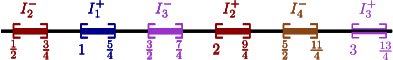
Figure 4.1: The intervals $I_{j}^{-}$, $I_{j}^{+}$ out of which we sample the levels. The fractions are in multiples of $n/r$.

The strategy goes as follows. For each index $i=2,\ldots,r-1$, consider the pair of levels $L_{k_{i}^{-}}$, $L_{k_{i}^{+}}$, which we denote shortly and respectively as $L_{i}^{-}$, $L_{i}^{+}$, and approximate both of them simultaneously, using the following refinement of the algorithm summarized in Theorem 3.1, with the same parameter $t=cn/r$ for all pairs, where $c\ll 1/4$ is a sufficiently small constant. Project $L_{i}^{-}$ and $L_{i}^{+}$ onto the $xy$-plane, and overlap the resulting planar maps $M_{i}^{-}$, $M_{i}^{+}$ into a single map $M_{i}^{*}$. Each vertex of $M_{i}^{*}$ is either the projection of a vertex of one of the levels $L_{i}^{-}$, $L_{i}^{+}$, or a crossing point of a pair of projected edges, one from each level.

We now apply the preceding analysis to $M_{i}^{*}$, and get a triangulation $T_{i}$ of the $xy$-plane, whose combinatorial complexity is $O(|M_{i}^{*}|/t^{2})$. We lift its vertices up to both levels $L_{i}^{-}$, $L_{i}^{+}$, resulting in a corresponding pair of triangulated terrains $T_{i}^{-}$, $T_{i}^{+}$, with identical $xy$-projections. We claim that $T_{i}^{-}$ approximates $L_{i}^{-}$ and $T_{i}^{+}$ approximates $L_{i}^{+}$. Indeed, each boundary edge of a piece of the $t^{2}$-division of $M_{i}^{*}$ is a portion of a projected edge of either $L_{i}^{-}$ or $L_{i}^{+}$. Hence, traversing any portion of the boundary of a piece, we encounter at most $O(t)$ edges of each of the levels $L_{i}^{-}$, $L_{i}^{+}$. Specifically, when we go along an edge of $M_{i}^{*}$ that is a portion of some edge of $M_{i}^{-}$, say, we do not cross any edge of $M_{i}^{+}$, so when we lift the edge to the “wrong” terrain ($L_{i}^{+}$ in this case), we get two points that lie on the same face, and the property follows. The arguments used above imply that, when lifted to either of the two levels, the crossing number of the corresponding path is at most $O(t)$, from which the claim follows. Each triangle $\Delta$ of $T_{i}$ is lifted to a pair of triangles $\Delta^{-}\in T_{i}^{-}$, $\Delta^{+}\in T_{i}^{+}$, and we connect them by a vertical triangular prism $\Delta^{*}$ that has them as its bases. These prisms are pairwise openly disjoint, and their union is the layer $\Lambda_{i}$ between $T_{i}^{-}$ and $T_{i}^{+}$. Let $\Xi_{i}$ denote the collection of these prisms.

For $i=1$ we project $L_{1}^{+}$, and apply the preceding analysis to the resulting planar maps $M_{1}^{+}$, and get a triangulation $T_{1}$ of size $O(|M_{1}|/t^{2})$. We lift $T_{1}$ up to $L_{1}^{+}$ and extend each triangle $\Delta$ of the lifted $T_{1}$ into a a semi-unbounded prism, $\Delta^{*}$, that contains all the points vertically below $\Delta$. We denote by $\Xi_{1}$ this collection of semi-unbounded prisms. We process $L_{r}^{-}$ analogously and obtain a collection $\Xi_{r}$ of semi-unbounded prisms that contain all points vertically above the resulting lifted triangulation $T_{r}$.

The union $\Xi=\bigcup_{i}\Xi_{i}$ of our collections of vertical prisms is the entire 3-space. These prisms are not pairwise openly disjoint, but each point in $\mathbb{R}^{3}$ is contained in the interiors of at most two prisms. Informally, the layers $\Lambda_{1},\ldots,\Lambda_{r}$ overlap in pairs (but no three layers overlap), so that each layer is fully triangulated by pairwise openly disjoint vertical prisms.

Lemma 4.3.

The expected size of $\Xi$ is $O(r^{3})$.

Proof:

The overall number of prisms in $\Xi$ is, by Theorem 3.1,

$$|\Xi|=O\left(\frac{1}{t^{2}}\sum_{i=1}^{r}|M_{i}^{*}|\right).$$ (4.1)

We have $|M_{i}^{*}|=O(|L_{i}^{-}|+|L_{i}^{+}|+|X_{i}|)$, where $X_{i}$ is the set of pairs $(e,e^{\prime})$ of edges, where $e$ is an edge of $L_{i}^{-}$, $e^{\prime}$ is an edge of $L_{i}^{+}$, and the $xy$-projections of $e$ and $e^{\prime}$ cross each other. For $i=1$ we formally define $M_{1}^{*}=M_{1}^{+}$ so $|M_{1}^{*}|=O(|L_{1}^{+}|)$ and for $i=r$ we define $M_{r}^{*}=M_{r}^{-}$ so $|M_{r}^{*}|=O(|L_{r}^{-}|)$.

Estimating $\sum_{i}(|L_{k_{i}^{-}}|+|L_{k_{i}^{+}}|)$ is easy. Each level of ${\cal A}(H)$ appears in this sum with probability at most $4r/n$ (note that some levels will never be chosen), so the expected value is at most proportional to $4r/n$ times the complexity of ${\cal A}(H)$, namely, $O((r/n)\cdot n^{3})=O(n^{2}r)$.

To estimate the expected value of $\sum_{i}|X_{i}|$, we note that each pair $(e,e^{\prime})$ that is counted in this sum belongs to the set, call it $X_{0}$, of pairs that are accounted for in the bound in Lemma 4.2, with $q=7n/(4r)$, but our pairs constitute only a small subset of $X_{0}$. Specifically, by our choice of random levels, the probability of a pair $(e,e^{\prime})\in X_{0}$ to appear in one of the sets $X_{i}$ is at most proportional to

$$(4r/n)^{2}\cdot|X_{0}|=O\left((r/n)^{2}\cdot n^{3}\cdot(n/r)\right)=O(n^{2}r).$$

Substituting the separate bounds obtained so far in Eq. (4.1), we get that the expected size of $\Xi$ satisfies

$$|\Xi|=O\left(\frac{1}{t^{2}}\sum_{i=1}^{r}|M_{i}^{*}|\right)=O\left(\frac{r^{2}}{n^{2}}\cdot n^{2}r\right)=O(r^{3}).$$

 

By applying this construction with $r^{\prime}=r/c$ instead of $r$, for some sufficiently large constant $c$, we can guarantee that each prism does not intersect more than $n/r$ planes, at the cost of increasing the number of prisms by a constant factor. We therefore obtain the following result.

Theorem 4.4.

For a set $H$ of $n$ non-vertical planes in $\mathbb{R}^{3}$ in general position, and a parameter $r<n$, one can construct a layered $(1/r)$-cutting of ${\cal A}(H)$ of size $O(r^{3})$. Specifically, we cover space by a set $\Xi$ of $O(r^{3})$ vertical triangular prisms, such that each point is covered at most twice, and each prism is crossed by $\leq n/r$ planes of $H$. The top triangles of the prisms form $r$ polyhedral terrains, each approximating a suitable level of ${\cal A}(H)$, and the bottom triangles of the prisms form $r$ other polyhedral terrains of a similar nature.

One can construct such a cutting efficiently by using a relative $\left(\frac{1}{r},\frac{1}{2}\right)$-approximation of size $O(r\log r)$ as in Section 3.2. We construct the arrangement ${\cal A}(S)$ of such a sample $S$, apply the construction as described above to obtain a $(1/r^{\prime})$-cutting of ${\cal A}(S)$ for $r^{\prime}=r/c$ where $c$ is a suitable fixed constant, and claim that this is, with probability $1-1/r^{O(1)}$, also $(1/r)$-cutting of ${\cal A}(H)$. It takes linear time to sample $S$ and then $O(|S|^{3})=O(r^{3}\log^{3}r)$ time to construct ${\cal A}(S)$ and apply to it the algorithm described above.

One can construct the conflict lists using a standard range reporting data structure. We preprocess $H$ into a data structure of size $s\geq n$, in time $O(s\cdot{\rm polylog}(n))$, so that, for each query segment $e$, we can report all the $k_{e}$ planes of $H$ that $e$ crosses in time $O(\frac{n}{s^{1/3}}{\rm polylog}(n))+k_{e})$; See [Mat92b, Cha12] for details. We query the structure with the $O(r^{3})$ edges of the prisms of the cutting, and assemble from the outputs, in a straightforward manner, the conflict lists of the prisms. The overall running time is $O((\frac{r^{3}n}{s^{1/3}}+s){\rm polylog}(n)+\sum_{e}k_{e})$. We have that $\sum_{e}k_{e}=O(r^{3}(n/r))=O(nr^{2})$. We choose $s=\max\{r^{9/4}n^{3/4},n\}$; this makes the running time $O(nr^{2}{\rm polylog}(n))$, as is easily checked.

4.2 Approximate halfspace range counting

In its dual setting, the problem is: Let $H$ be a set of $n$ nonvertical planes in $\mathbb{R}^{3}$ in general position, and let ${\varepsilon}>0$ be an error parameter. We wish to preprocess $H$ into a data structure that supports queries of the form: For a query point $q$, count the number of planes lying below $q$, up to a multiplicative factor of $1\pm{\varepsilon}$. That is, if $q$ lies at level $k$, the answer should be between $(1-{\varepsilon})k$ and $(1+{\varepsilon})k$.

Let $m=O(1/{\varepsilon}^{4/3})$. We construct and store the first $m$ levels of ${\cal A}(H)$ explicitly, each level as its own terrain. Formally, for $j=0,\ldots,m$, we set $k_{j}=j$, and compute level $j$, denoted by $T^{\prime}_{j}$, and its $xy$-projection denoted by $T_{j}$. Next, for deeper levels, we use the approximate level construction. We take the sequence of levels $k_{m+i}:=m(1+{\varepsilon})^{i}$, for $i=1,\ldots,m^{\prime}$, where $m^{\prime}=\left\lceil{\log_{1+{\varepsilon}}\frac{n}{m}}\right\rceil\approx\frac{1}{{\varepsilon}}\log n.$ For each $i=m+1,\ldots,m+m^{\prime}$, approximate level $L_{k_{i}}$ up to an additive error of ${\varepsilon}k_{i}$, let $T_{i}$ denote the underlying triangulation in the $xy$-plane of the projection of the approximation, and let $T^{\prime}_{i}$ denote the approximating terrain, namely, the appropriate lifting of $T_{i}$. By construction, it is easily checked that the terrains $T^{\prime}_{i}$ do not cross one another, and are therefore stacked on top of one another. To answer an approximate (dual) halfspace range counting query with a point $q$, we simply need to find two consecutive terrains $T^{\prime}_{i}$, $T^{\prime}_{i+1}$ between which $q$ lies, and return $m(1+{\varepsilon})^{i-m}$, say, as the approximate count, when $i>m$, or $i$ itself otherwise. For this we also construct a point location data structure over the xy-projection of each of the first $m$ levels and over $T_{i}$ for $i=1,\ldots,m^{\prime}$.

By Theorem 3.1, for $i=1,\ldots,m^{\prime}$, the complexity of $T_{m+i}$ (and of $T^{\prime}_{m+i})$ is

$$|T_{m+i}|=O\left({\frac{n}{{\varepsilon}^{3}k_{m+i}}}\right)=O\left({\frac{n}{{\varepsilon}^{3}m(1+{\varepsilon})^{i}}}\right).$$

Summing these bounds over $i$, we get

$$\sum_{i=1}^{m^{\prime}}\left|{T_{m+i}}\right|=O\left({\frac{n}{{\varepsilon}^{3}m}}\right)\sum_{i=1}^{m^{\prime}}\frac{1}{(1+{\varepsilon})^{i}}=O\left({\frac{n}{{\varepsilon}^{4}m}}\right).$$

Storing the first $m$ levels of ${\cal A}(G)$ requires $O(nm^{2})$ space (this bounds their overall complexity), so both bounds are $O(n/{\varepsilon}^{8/3})$, for $m=O(1/{\varepsilon}^{4/3})$. This bounds the storage used by our data structure. To construct the data structure we spend $O(n\log n+nm^{2})$ time to construct the first $m$ levels [Cha00], and $O(nm^{2}\log n)$ time for the point location data structures over the projections of the first $m$ levels. Then, by Theorem 3.3, we spend $O(n+{\varepsilon}^{-6}\sum r_{i}\log^{3}r_{i})$ time to construct the approximate levels $T^{\prime}_{i}$, for $i=1,\ldots,m^{\prime}$, where $r_{i}=n/k_{m+i}$. (The additive factor of $n$ in Theorem 3.3 accounts for the time it takes to draw the appropriate sample of $\frac{br_{i}}{\epsilon^{2}}\log r_{i}$ planes. It appear once in the bound above since we can draw all samples simultaneously.) Since $r_{i}=n/k_{m+i}=\frac{n}{m(1+{\varepsilon})^{i}}$, it follows that $\sum r_{i}=O(\frac{n}{m{\varepsilon}})=O(n{\varepsilon}^{1/3})$ so the total time we spend for constructing the approximate levels $T^{\prime}_{i}$, for $i=1,\ldots,m^{\prime}$ is $O({\varepsilon}^{-5\frac{2}{3}}n\log^{3}n)$. This includes the time it takes to construct a point location data structure over $T_{i}$ and dominates the total preprocessing time.

To answer a query with some point $q$, we run a binary search over the terrains $T^{\prime}_{i}$, and locate the $xy$-projection of $q$ in the relevant planar maps $T_{i}$, thereby determining whether $q$ lies above or below $T^{\prime}_{i}$. The total cost of a query is therefore

$$O\left({\log\left(\frac{1}{{\varepsilon}}\log n\right)\cdot\log n}\right).$$

Afshani and Chan [AC09a] showed how to avoid the binary search for finding the right level, using a data structure of Kaplan et al. [KRS11]. Afshani and Chan use this latter structure to find a rough approximation to the level. Specifically, they find an estimate $\hat{\ell}$ to the level $k$ of $q$ such that the probability that $\hat{\ell}$ is off by a factor of (at least) $b$ from $k$ is $O(1/b)$. Then, instead of doing a binary search, they linearly search for the right level, starting from the level in the hierarchy closest to $\hat{\ell}$. The expected number of searches that they perform is then $O(1)$ and these searches take $O(\log(n/({\varepsilon}k))$ time since each is a point location query over an arrangement of size $O(n/({\varepsilon}^{3}k))$. We can apply the exact same technique using our approximate levels instead of the more complicated refined shallow cuttings used in [AC09a], and then get the following.

Theorem 4.5.

Let $H$ be a set of $n$ nonvertical planes in $\mathbb{R}^{3}$, and let ${\varepsilon}>0$ be a prescribed parameter. Ome can then construct a data structure of size $O(n/{\varepsilon}^{8/3})$, in near-linear expected time, and that can answer approximate level queries in ${\cal A}(H)$, up to a relative error of ${\varepsilon}$, in $O(\log(n/({\varepsilon}k)))$ expected time, where $k$ is the exact level of the query.

Acknowledgments. We thank János Pach for pointing out that a variant of Theorem 2.3 is already known.

[autoplay,autoresume,width=0.9controls,loop,buttonsize=4em]2figs/animation_1022

Figure 4.2: Animation of algorithm – you would need Acrobat reader to see the animation - click the figure to make it start.

References

- [AACS98] P. K. Agarwal, B. Aronov, T. M. Chan, and M. Sharir. On levels in arrangements of lines, segments, planes, and triangles. Discrete Comput. Geom., 19:315–331, 1998.
- [AC09a] P. Afshani and T. M. Chan. On approximate range counting and depth. Discrete Comput. Geom., 42(1):3–21, 2009.
- [AC09b] P. Afshani and T. M. Chan. Optimal halfspace range reporting in three dimensions. In Proc. 20th ACM-SIAM Sympos. Discrete Algs. (SODA), pages 180–186, 2009.
- [ACT14] P. Afshani, T. M. Chan, and K. Tsakalidis. Deterministic rectangle enclosure and offline dominance reporting on the RAM. In Proc. 41st Internat. Colloq. Automata Lang. Prog. (ICALP), volume 8572 of Lect. Notes in Comp. Sci., pages 77–88. Springer, 2014.
- [AD97] P. K. Agarwal and P. K. Desikan. An efficient algorithm for terrain simplification. In Proc. 8th ACM-SIAM Sympos. Discrete Algs. (SODA), pages 139–147, 1997.
- [AdBES14] B. Aronov, M. de Berg, E. Ezra, and M. Sharir. Improved bounds for the union of locally fat objects in the plane. SIAM J. Comput., 43(2):543–572, 2014.
- [AE99] P. K. Agarwal and J. Erickson. Geometric range searching and its relatives. In B. Chazelle, J. E. Goodman, and R. Pollack, editors, Advances in Discrete and Computational Geometry, pages 1–56. Amer. Math. Soc., Providence, RI, 1999.
- [Aga90a] P. K. Agarwal. Partitioning arrangements of lines I: an efficient deterministic algorithm. Discrete Comput. Geom., 5:449–483, 1990.
- [Aga90b] P. K. Agarwal. Partitioning arrangements of lines: II. Applications. Discrete Comput. Geom., 5:533–573, 1990.
- [Aga91a] P. K. Agarwal. Geometric partitioning and its applications. In J. E. Goodman, R. Pollack, and W. Steiger, editors, Computational Geometry: Papers from the DIMACS Special Year, pages 1–37. Amer. Math. Soc., Providence, RI, 1991.
- [Aga91b] P. K. Agarwal. Intersection and Decomposition Algorithms for Planar Arrangements. Cambridge University Press, New York, 1991.
- [AM95] P. K. Agarwal and J. Matoušek. Dynamic half-space range reporting and its applications. Algorithmica, 13:325–345, 1995.
- [AMS94] B. Aronov, J. Matoušek, and M. Sharir. On the sum of squares of cell complexities in hyperplane arrangements. J. Combinat. Theory Ser. A, 65:311–321, 1994.
- [AT14] P. Afshani and K. Tsakalidis. Optimal deterministic shallow cuttings for 3d dominance ranges. In Proc. 25th ACM-SIAM Sympos. Discrete Algs. (SODA), pages 1389–1398, 2014.
- [BR52] R. P. Bambah and C. A. Rogers. Covering the plane with convex sets. J. London Math. Soc., s1-27(3):304–314, 1952.
- [CEG+90] K. L. Clarkson, H. Edelsbrunner, L. J. Guibas, M. Sharir, and E. Welzl. Combinatorial complexity bounds for arrangements of curves and spheres. Discrete Comput. Geom., 5:99–160, 1990.
- [CEGS91] B. Chazelle, H. Edelsbrunner, L. J. Guibas, and M. Sharir. A singly-exponential stratification scheme for real semi-algebraic varieties and its applications. Theoret. Comput. Sci., 84:77–105, 1991. Also in Proc. 16th Int. Colloq. on Automata, Languages and Programming, pages 179–193, 179–193.
- [CF90] B. Chazelle and J. Friedman. A deterministic view of random sampling and its use in geometry. Combinatorica, 10(3):229–249, 1990.
- [Cha93] B. Chazelle. Cutting hyperplanes for divide-and-conquer. Discrete Comput. Geom., 9(2):145–158, 1993.
- [Cha00] T. M. Chan. Random sampling, halfspace range reporting, and construction of -levels in three dimensions. SIAM J. Comput., 30(2):561–575, 2000.
- [Cha04] B. Chazelle. Cuttings. In D. P. Mehta and S. Sahni, editors, Handbook of Data Structures and Applications, chapter 25. Chapman and Hall/CRC, Boca Raton, Florida, 2004.
- [Cha05] T. M. Chan. Low-dimensional linear programming with violations. SIAM J. Comput., 34(4):879–893, 2005.
- [Cha10] T. M. Chan. A dynamic data structure for 3-d convex hulls and 2-d nearest neighbor queries. J. Assoc. Comput. Mach., 57(3):1–15, 2010. Art. 16.
- [Cha12] T. M. Chan. Optimal partition trees. Discrete Comput. Geom., 47(4):661–690, 2012.
- [Cla87] K. L. Clarkson. New applications of random sampling in computational geometry. Discrete Comput. Geom., 2:195–222, 1987.
- [CS89] K. L. Clarkson and P. W. Shor. Applications of random sampling in computational geometry, II. Discrete Comput. Geom., 4:387–421, 1989.
- [CT15] T. M. Chan and K. Tsakalidis. Optimal deterministic algorithms for 2-d and 3-d shallow cuttings. In Proc. 31st Int. Annu. Sympos. Comput. Geom. (SoCG), pages 719–732, 2015.
- [EHS04] E. Ezra, D. Halperin, and M. Sharir. Speeding up the incremental construction of the union of geometric objects in practice. Comput. Geom. Theory Appl., 27(1):63–85, 2004.
- [Fre87] G. N. Frederickson. Fast algorithms for shortest paths in planar graphs, with applications. SIAM J. Comput., 16(6):1004–1022, 1987.
- [Har00] S. Har-Peled. Constructing planar cuttings in theory and practice. SIAM J. Comput., 29(6):2016–2039, 2000.
- [HKS16] S. Har-Peled, H. Kaplan, and M. Sharir. Approximating the k-level in three-dimensional plane arrangements. In Proc. 27th ACM-SIAM Sympos. Discrete Algs. (SODA), pages 1193–1212, 2016.
- [HS11] S. Har-Peled and M. Sharir. Relative -approximations in geometry. Discrete Comput. Geom., 45(3):462–496, 2011.
- [KLPS86] K. Kedem, R. Livne, J. Pach, and M. Sharir. On the union of Jordan regions and collision-free translational motion amidst polygonal obstacles. Discrete Comput. Geom., 1:59–71, 1986.
- [KMS13] P. N. Klein, S. Mozes, and C. Sommer. Structured recursive separator decompositions for planar graphs in linear time. In Proc. 45th Annu. ACM Sympos. Theory Comput. (STOC), pages 505–514, 2013.
- [Kol04] V. Koltun. Almost tight upper bounds for vertical decompositions in four dimensions. J. Assoc. Comput. Mach., 51(5):699–730, 2004.
- [KRS11] H. Kaplan, E. Ramos, and M. Sharir. Range minima queries with respect to a random permutation, and approximate range counting. Discrete Comput. Geom., 45(1):3–33, 2011.
- [KS05] V. Koltun and M. Sharir. Curve-sensitive cuttings. SIAM J. Comput., 34(4):863–878, 2005.
- [LT79] R. J. Lipton and R. E. Tarjan. A separator theorem for planar graphs. SIAM J. Appl. Math., 36:177–189, 1979.
- [Mat90] J. Matoušek. Construction of -nets. Discrete Comput. Geom., 5:427–448, 1990.
- [Mat92a] J. Matoušek. Efficient partition trees. Discrete Comput. Geom., 8:315–334, 1992.
- [Mat92b] J. Matoušek. Range searching with efficient hierarchical cutting. Discrete Comput. Geom., 10:157–182, 1992.
- [Mat92c] J. Matoušek. Reporting points in halfspaces. Comput. Geom. Theory Appl., 2(3):169–186, 1992.
- [Mat98] J. Matoušek. On constants for cuttings in the plane. Discrete Comput. Geom., 20:427–448, 1998.
- [Mil86] G. L. Miller. Finding small simple cycle separators for 2-connected planar graphs. J. Comput. Syst. Sci., 32(3):265–279, 1986.
- [MMP+91] J. Matoušek, N. Miller, J. Pach, M. Sharir, S. Sifrony, and E. Welzl. Fat triangles determine linearly many holes. In Proc. 32nd Annu. IEEE Sympos. Found. Comput. Sci. (FOCS), pages 49–58, 1991.
- [MRR14] N. H. Mustafa, R. Raman, and S. Ray. Settling the APX-hardness status for geometric set cover. In Proc. 55th Annu. IEEE Sympos. Found. Comput. Sci. (FOCS), pages 541–550, 2014.
- [Mul94] K. Mulmuley. An efficient algorithm for hidden surface removal, II. J. Comput. Syst. Sci., 49:427–453, 1994.
- [PA95] J. Pach and P. K. Agarwal. Combinatorial Geometry. John Wiley & Sons, New York, 1995.
- [Ram99] E. A. Ramos. On range reporting, ray shooting and k-level construction. In Proc. 15th Annu. Sympos. Comput. Geom. (SoCG), pages 390–399. ACM, 1999.
- [SA95] M. Sharir and P. K. Agarwal. Davenport-Schinzel Sequences and Their Geometric Applications. Cambridge University Press, New York, 1995.
- [Sei91] R. Seidel. A simple and fast incremental randomized algorithm for computing trapezoidal decompositions and for triangulating polygons. Comput. Geom. Theory Appl., 1:51–64, 1991.
\animategraphics[autoplay,autoresume,width=0.9controls,loop,buttonsize=4em]2figs/animation_1022