Evolution of coherence and non-classicality under global environmental interaction

Abstract

A master equation has been constructed for a global system-bath interaction both in the absence as well as presence of non-Markovian noise. For the memoryless case, it has been exactly solved for a paradigmatic class of two qubit states in high and zero temperature thermal environment. For the non-Markovian model, it has been solved for zero temperature bath. The evolution of quantum coherence and entanglement has been observed in presence of the above mentioned interactions. We show that the global part of the system-bath interaction compensates for the decoherence, resulting in slow down of coherence and entanglement decay. For an appropriately defined limiting case, both coherence and entanglement show freezing behaviour for the high temperature bath. In case of zero temperature bath, the mentioned interaction not only stabilizes the non-classical correlations, but also enhances them for a finite period. For the memory dependent case, we have seen that the global interaction enhances the back-flow of information from environment to the system, as it enhances the regeneration of coherence and entanglement. Also we have studied the generation of Quantum Fisher information by the mentioned process. An intuitive measure of non-classicality based on non-commutativity of quantum states has been considered. Bounds on generated quantum Fisher information has been found in terms of quantumness and coherence. This gives us a novel understanding of Quantum Fisher information as a measure of non-classicality.

PACS numbers: 03.65.Yz, 03.65.Ta

I Introduction

The main objective of the theory of open quantum systems is to develop a comprehensive description of various kind of interactions of the system with its ambient environment and their effect on the dynamics of the system of interest breuer ; weiss . Any realistic quantum system is bound to get affected by its environment and therefore the dynamical features of open quantum systems are particularly important from the practical perspective. Due to the advent of quantum technologies such as quantum communication teleport ; comm1 ; comm2 , quantum cryptography nelson ; crypto , there has been an upsurge of interest in the application of several techniques of open quantum systems. Markovian dynamics of open systems have been extensively studied and implemented successfully in a wide variety of problems breuer ; gp ; sgad ; qw ; wigner ; tomo .

However, due to impressive developments in the experimentation with quantum systems and their control control , it has been realized that open quantum systems do not generally behave within the domain of Markovian dynamics sg ; qbm . Particularly for the case of systems constituting more than one interacting sub-systems, where the interactions between the parties may be comparable to the interaction strength of the coupling to the bath, it is natural for the dynamics to deviate from Markovian behavior fleming . Effects of non-Markovian structured environment on quantum coherence and correlation has been theoretically and experimentally studied franco1 ; franco2 ; franco3 ; franco4 ; franco5 . A number of measures of deviation from Markovianity have been proposed recently, where “Non-Markovianity” is recognized as the departure from monotonic behavior of certain measures under strictly Markovian dynamics wolf ; breuer2 ; laine ; rivas ; raja ; breuer3 ; s1 ; s2 ; s3 . Generally, a quantitative measure, which shows monotonic behavior under Markovian dynamics is addressed and departure from that monotonicity is taken to be a signature of non-Markovianity. For example, we can consider the dynamics of entanglement in an open system scenario. Since local trace preserving completely positive maps do not increase the amount of entanglement, evidently it can be surmised that the entanglement with an ancillary system decays monotonically within Markovian regime. Thus, for example, in Ref. rivas the dynamics of entanglement was used as a signature to identify the non-Markovian characteristics of a system-environment interaction.

In recent times, the theory of quantum coherence as a resource has attracted much attention plenio ; winter1 ; uttam1 ; uttam2 ; uttam3 ; manab1 ; rana1 ; strelsov . Coherence plays a central role in quantum mechanics enabling operations or tasks which are impossible within the regime of classical mechanics. Coherence underlies the non-classical behavior of a quantum system, like entanglement. In Ref. plenio several measures, like the $l_{1}$ norm and the relative entropy were introduced to characterize the coherence of a quantum system. The valid measures of coherence should not increase under allowed incoherent operations. Based on this, it can be inferred that the measures of quantum coherence are monotone under Markovian dynamics. Hence any deviation from the montonicity of coherence measure can also be taken as a signature of deviation from Markovian dynamics titas ; ning . The central theme of our work revolves around this specific issue of the dynamical behavior of coherence monotones under a specific system-environment interaction which is not strictly Markovian. Usually for the case of Markovian dynamics of a composite system, the environment acts locally on each of the parties. For the bipartite case, considered here, the environment is globally interacting with the system. This enables us to consider two parts of the non-unitary evolution. One is of course the local Lindbladian and the other is an interactive part which is essentially causing the deviation from Markovian evolution. Here we have taken a two qubit atomic system interacting with a Harmonic oscillator bath. A similar model with a squeezed thermal bath has been studied earlier for estimating the entanglement dynamics of the atomic system banerjee ; tanas . Based on the above mentioned model, the first part of our work is to present an analytical estimation of the dynamics of coherence, for the purpose of characterization of the deviation from monotonicity and to find the conditions under which such deviation occurs. After that we will extend our study to calculate the exact expression of concurrence for a special class of two qubit X states in order to observe the dynamics of entanglement in our proposed system-bath interaction.

Next, we consider the generation of quantum Fisher information by the global environmental interaction. The Fisher information is a measure of intrinsic accuracy in statistical ensemble theory fisher ; crammer-rao . Quantum generalization of the Fisher information has also been introduced helstrom ; holevo , which can be considered as a measure of non-classicality for quantum system hall ; sbomkar . A measure of quantumness has been proposed in a recent work vedral , based on the non-commutativity of quantum states. We have shown that the Quantum Fisher information is lower bounded by the above mentioned quantumness with a factor of 1/4 and upper bounded by the $l_{1}$ norm of coherence with a factor of 1/2. This gives us an intuitive understanding of Quantum Fisher information as a measure of non-classicality. We have estimated the amount of quantumness and Fisher information that can be generated by the global environmental interaction. Then, we extend our study by considering the memory effect of environmental interaction. We have used a non-Markovian noise model to generalize the global master equation for memory dependent system-bath interactions. We also solve the master equation for two qubit X states to obtain analytical expressions for the $l_{1}$ norm of coherence and concurrence and study their dynamics. Further we also investigate the generation of quantumness in the memory dependent environmental interaction.

The organisation of the paper is as follows. In Section II, we will construct the master equation of the concerned system and obtain analytical solution for a particular class of density matrices. In Sections III and IV, we discuss the dynamics of quantum coherence, concurrence quantum Fisher information and quantumness, respectively. In Section V we generalize the master equation to incorporate memory dependent environmental interactions. We then present our conclusions in Section VI.

II Dynamics of composite quantum system in global environmental interaction

The dynamics of the reduced density matrix of the system of interest, undergoing a completely positive (CP) evolution, can be expressed in terms of the Kraus operator sum representation (OSR) as

$$\rho(t)=\sum_{i}M_{i}(t)\rho(0)M_{i}^{\dagger}(t).$$ (1)

The Kraus operators $M_{i}$ must satisfy the trace preserving condition, i.e.,

$$\sum_{i}M_{i}^{\dagger}(t)M_{i}(t)=\mathbb{I}.$$ (2)

The Kraus operator sum representation governs a CP evolution. The Markovian master equation can be constructed from the Kraus representation preskill . For a small time interval $\delta t$, if we consider

$$\begin{array}[]{ll}M_{i}(t)\approx\sqrt{\delta t}L_{i},~{}~{}~{}~{}~{}\forall~{}i\neq 0\\ M_{0}(t)\approx\mathbb{I}-\frac{\delta t}{2}\sum_{i\neq 0}L_{i}^{\dagger}L_{i},\end{array}$$ (3)

then it can be seen from equation (1), that

$$\frac{\rho(t)-\rho(0)}{\delta t}=\sum_{i}\left[L_{i}\rho L_{i}^{\dagger}-\frac{1}{2}\left(L_{i}^{\dagger}L_{i}\rho+\rho L_{i}^{\dagger}L_{i}\right)\right].$$ (4)

Now if we consider $L_{i}=\sqrt{\gamma_{i}}A_{i}$ , then for $\delta t\rightarrow 0$, we get the differential equation

$$\frac{d\rho}{dt}=\sum_{i}\gamma_{i}\left[A_{i}\rho A_{i}^{\dagger}-\frac{1}{2}\left(A_{i}^{\dagger}A_{i}\rho+\rho A_{i}^{\dagger}A_{i}\right)\right],$$ (5)

where $\gamma_{i}$s are the decay parameters. This is basically the usual Markovian master equation. Following Ref. lider , for a fixed operator basis $\{A_{\alpha}\}_{\alpha=0}^{n}$, with $A_{0}=\mathbb{I}$, we can define $L_{i}=\sum_{\alpha=0}^{n}b_{i\alpha}A_{\alpha}$. Using equation (3), it can be seen that the master equation becomes

$$\frac{d\rho}{dt}=\sum_{\alpha,\beta}\gamma_{\alpha\beta}\left[A_{\alpha}\rho A_{\beta}^{\dagger}-\frac{1}{2}\left(A_{\alpha}^{\dagger}A_{\beta}\rho+\rho A_{\alpha}^{\dagger}A_{\beta}\right)\right],$$ (6)

where $\{\gamma_{\alpha\beta}=\sum_{i}b_{i\alpha}b_{i\beta}^{*}\}$ represents a coefficient matrix, called as the damping basis. The positivity of this kind of dynamical map depends on the positivity of the $\{\gamma_{\alpha\beta}\}$ matrix lider . If all the eigenvalues of the damping basis matrix are positive, then the map is completely positive.

Here we are dealing with a two qubit atomic system. Let us first begin by writing down the master equation for such systems, which is of the form (5)

$$\frac{d\rho}{dt}=\sum_{i=1,2}\gamma_{i}(N+1)\left(\sigma_{i}^{-}\rho\sigma_{i}^{+}-\frac{1}{2}\left(\sigma_{i}^{+}\sigma_{i}^{-}\rho+\rho\sigma_{i}^{+}\sigma_{i}^{-}\right)\right)+\sum_{i=1,2}\gamma_{i}N\left(\sigma_{i}^{+}\rho\sigma_{i}^{-}-\frac{1}{2}\left(\sigma_{i}^{-}\sigma_{i}^{+}\rho+\rho\sigma_{i}^{-}\sigma_{i}^{+}\right)\right),$$ (7)

where

$$N=\frac{1}{\exp(\frac{\hbar\omega}{k_{B}T})-1},$$ (8)

is the Planck distribution function and

$$\begin{array}[]{ll}\sigma_{1}^{-}=\sigma^{-}\otimes\mathbb{I}~{}~{};~{}~{}\sigma_{1}^{+}=\sigma^{+}\otimes\mathbb{I},\\ \sigma_{2}^{-}=\mathbb{I}\otimes\sigma^{-}~{}~{};~{}~{}\sigma_{2}^{+}=\mathbb{I}\otimes\sigma^{+},\end{array}$$ (9)

are the dipole lowering and raising operators acting locally on the two parties.
Let us now generalize this master equation for the two qubit system following banerjee , where the environment is modelled as a thermal radiation field, which is interacting with the system in a global way. This is achieved by a coupling dependent upon the qubit position $\bf{r}_{n}$. The effective Hamiltonian of the two qubit system can be expressed as

$$H_{S}=\sum_{n=1,2}\hbar\omega_{n}\sigma^{z}_{n}+H_{int},$$ (10)

with

$$H_{int}=\hbar\left(\Omega_{21}\sigma^{-}\otimes\sigma^{+}+\Omega_{12}\sigma^{+}\otimes\sigma^{-}\right)$$ (11)

where

$$\Omega_{ij}=\frac{3}{4}\sqrt{\gamma_{i}\gamma_{j}}\left[-(1-(\hat{\mu}.\hat{r}_{ij})^{2})\frac{\cos k_{0}r_{ij}}{k_{0}r_{ij}}+(1-3(\hat{\mu}.\hat{r}_{ij})^{2})\left[\frac{\sin k_{0}r_{ij}}{(k_{0}r_{ij})^{2}}+\frac{\cos k_{0}r_{ij}}{(k_{0}r_{ij})^{3}}\right]\right].$$ (12)

Here $\hat{\mu}=\hat{\mu}_{1}=\hat{\mu}_{2}$ are the dipole moment operators and $\hat{r_{ij}}$ are the unit vectors along the atomic transition dipole moments with $\bf{r}_{ij}=\bf{r}_{i}-\bf{r}_{j}$. Also $k_{0}=\omega_{0}/c$, where $\omega_{0}=(\omega_{1}+\omega_{2})/2$ and $\gamma_{i}=\omega_{i}^{3}\mu_{i}^{2}/3\pi\varepsilon\hbar c^{3}$ is the spontaneous emission rate. Following Ref. banerjee , the non-unitary part of the global master equation can be written as

$$\frac{d\rho}{dt}=\frac{i}{\hbar}[\rho,H_{S}]+\sum_{i,j=1,2}\gamma_{ij}(N+1)\left(\sigma_{i}^{-}\rho\sigma_{j}^{+}-\frac{1}{2}\left(\sigma_{i}^{+}\sigma_{j}^{-}\rho+\rho\sigma_{i}^{+}\sigma_{j}^{-}\right)\right)+\sum_{i,j=1,2}\gamma_{ij}N\left(\sigma_{i}^{+}\rho\sigma_{j}^{-}-\frac{1}{2}\left(\sigma_{i}^{-}\sigma_{j}^{+}\rho+\rho\sigma_{i}^{-}\sigma_{j}^{+}\right)\right),$$ (13)

where

$$\begin{array}[]{ll}\gamma_{ij}=\sqrt{\gamma_{i}\gamma_{j}}\large{a}(k_{0}r_{ij})~{};~{}~{}~{}\forall i\neq j\\ \gamma_{i}=\frac{\omega_{i}^{3}\mu_{i}^{2}}{3\pi\varepsilon\hbar c^{3}},\end{array}$$ (14)

with

$$a(k_{0}r_{ij})=\frac{3}{2}\left[(1-(\hat{\mu}.\hat{r}_{ij})^{2})\frac{\sin k_{0}r_{ij}}{k_{0}r_{ij}}+(1-3(\hat{\mu}.\hat{r}_{ij})^{2})\left[\frac{\cos k_{0}r_{ij}}{(k_{0}r_{ij})^{2}}-\frac{\sin k_{0}r_{ij}}{(k_{0}r_{ij})^{3}}\right]\right].$$ (15)

The interaction Hamiltonian $H_{int}$ with characteristic frequency $\Omega_{ij}$ governs the coherent part of the evolution and the non-unitary part with characteristic frequency $\gamma_{ij}$ regulates the incoherent part of the evolution. Note that, $\gamma_{ij}$ arises due to multi qubit interaction of the composite system with the bath and is the reason behind the global nature of the system-bath interaction. Basically, the bath opens up a channel between the two system qubits, an aspect of global interaction not seen for local interactions. It is to be noted that both $\Omega_{ij}$ and $\gamma_{ij}$ are environment dependent, where the environment factor of $\Omega_{ij}$ is described by the elements in the square brackets of Eq. (12) and the corresponding factor of $\gamma_{ij}$ comes from the parameter $a(k_{0}r_{ij})$ in Eq. (15) quantifying the coupling between qubits and bath.

For a two qubit system with identical parties we have $\gamma_{12}=\gamma_{21}$ and $\gamma_{1}=\gamma_{2}=\gamma$. Also, $k_{0}=2\pi/\lambda_{0}$ is the resonant wave vector, and occurring in the term $k_{0}r_{ij}$ indicates a resonant length scale. Now the damping basis matrix for the equation (13) will be

$$\left(\begin{matrix}\gamma(N+1)~{}~{}0~{}~{}\gamma_{12}(N+1)~{}~{}0\\ 0~{}~{}~{}~{}~{}~{}~{}~{}\gamma N~{}~{}~{}~{}~{}0~{}~{}~{}~{}~{}~{}~{}~{}\gamma_{12}N\\ \gamma_{12}(N+1)~{}0~{}~{}\gamma(N+1)~{}0\\ 0~{}~{}~{}~{}~{}\gamma_{12}N~{}~{}~{}~{}~{}~{}0~{}~{}~{}~{}~{}~{}\gamma N\\ \end{matrix}\right).$$ (16)

From (16), we see that the condition for positivity is $\gamma_{12}\leq\gamma$, that is, $a(k_{0}r_{ij})\leq 1$ (for the rest of the paper we will denote it by $a$). Using (15), we find the specific condition for positivity as

$$R\sin^{2}\phi\frac{\sin(k_{0}r_{ij}-\theta)}{k_{0}r_{ij}}\leq\frac{2}{3},$$ (17)

with

$$R=\sqrt{\left(1+\frac{2\cot^{2}\phi-1}{(k_{0}r_{ij})^{2}}\right)^{2}+\left(\frac{2\cot^{2}\phi-1}{k_{0}r_{ij}}\right)^{2}},$$ (18)

and

$$\tan\theta=\frac{2\cot^{2}\phi-1}{k_{o}r_{ij}+\frac{2\cot^{2}\phi-1}{k_{0}r_{ij}}}.$$ (19)

For a specific case, we can take $\cot\phi=1/\sqrt{2}$, so that $\tan\theta=0$ and $R=1$. For this case, the condition of positivity reduces to

$$\frac{\sin k_{0}r_{ij}}{k_{0}r_{ij}}\leq 1.$$ (20)

From (20), it is evident that the limiting condition $(a\rightarrow 1)$ can be reached, when the separation ($r_{ij}$) is very small compared to the resonant wavelength $\lambda_{0}$. This is attainable when $\lambda_{0}$ is very large, i.e., the separation between the energy levels of both the atomic qubits is small. Our aim here is to find a solution for the master equation given by (13). For that purpose we take a special class of density matrices of the form of X-states

$$\left(\begin{matrix}\rho_{11}~{}~{}0~{}~{}0~{}~{}\rho_{14}\\ ~{}0~{}\rho_{22}~{}~{}\rho_{23}~{}0\\ ~{}0~{}\rho_{23}^{*}~{}~{}\rho_{33}~{}0\\ \rho_{14}^{*}~{}~{}0~{}~{}0~{}~{}\rho_{44}\\ \end{matrix}\right).$$ (21)

X states are very important in the study of quantum information theory because of their simple representation x1 ; x2 . This class includes, among others, the well-known Bell diagonal and Werner states. X states has been studied extensively in the literature (x1, ; x2, ). Their invariance properties and the underlying symmetry have been studied (x2, ). It has been shown that they remain form invariant under the considered quantum operations. Inserting (21) in (13), we get the following set of coupled differential equations

$$\begin{array}[]{ll}\dot{\rho}_{11}=-2\gamma(N+1)\rho_{11}+\gamma N(\rho_{22}+\rho_{33})+\gamma_{12}N(\rho_{23}+\rho_{23}^{*}),\\ \dot{\rho}_{22}=\gamma(N+1)\rho_{11}+\gamma N\rho_{44}-\gamma(2N+1)\rho_{22}\\ ~{}~{}~{}~{}~{}~{}~{}~{}-\frac{\gamma_{12}}{2}(2N+1)(\rho_{23}+\rho_{23}^{*})+i\Omega_{12}(\rho_{23}-\rho_{23}^{*}),\\ \dot{\rho}_{33}=\gamma(N+1)\rho_{11}+\gamma N\rho_{44}-\gamma(2N+1)\rho_{22}\\ ~{}~{}~{}~{}~{}~{}~{}~{}-\frac{\gamma_{12}}{2}(2N+1)(\rho_{23}+\rho_{23}^{*})-i\Omega_{12}(\rho_{23}-\rho_{23}^{*}),\\ \dot{\rho}_{44}=-(\dot{\rho}_{11}+\dot{\rho}_{22}+\dot{\rho}_{33}),\\ \dot{\rho}_{23}=-\gamma(2N+1)\rho_{23}+\gamma_{12}(N+1)\rho_{11}+\gamma_{12}N\rho_{44}\\ ~{}~{}~{}~{}~{}~{}~{}~{}-\frac{\gamma_{12}}{2}(2N+1)(\rho_{22}+\rho_{33})+i\Omega_{12}(\rho_{22}-\rho_{33}),\\ \dot{\rho}_{14}=-\gamma(2N+1)\rho_{14}-4i\omega\rho_{14}.\end{array}$$ (22)

We are going to solve this for two cases of high and zero temperature.

II.1 High temperature case

For the case when the thermal bath is at high temperature ($N>>1$), the rates of dissipation and absorption are equal. The solution of the master equation is then given by

$$\begin{array}[]{ll}\rho_{11}(t)=W(t)+W^{\prime}(t),~{}\rho_{44}(t)=W(t)-W^{\prime}(t),\\ \rho_{22}(t)=U(t)+U(^{\prime}t),~{}\rho_{33}(t)=U(t)-U^{\prime}(t),\\ \rho_{23}=V(t)+iV^{\prime}(t),\rho_{14}(t)=\rho_{14}(0)\exp\left[-\left(2\gamma N+4i\omega\right)t\right].\end{array}$$ (23)

where

$$\begin{array}[]{ll}W(t)=\frac{W(0)+U(0)}{2}-\left(\frac{U(0)-W(0)}{2}\right)e^{-3\gamma Nt}\left[\cosh\left(\gamma Nt\sqrt{1+8a^{2}}\right)-\frac{\sinh\left(\gamma Nt\sqrt{1+8a^{2}}\right)}{\sqrt{1+8a^{2}}}\right]\\ ~{}~{}~{}~{}~{}~{}~{}~{}+\frac{2a}{\sqrt{1+8a^{2}}}V(0)e^{-3\gamma Nt}\sinh\left(\gamma Nt\sqrt{1+8a^{2}}\right),\end{array}$$ (24)

$$\begin{array}[]{ll}U(t)=\frac{W(0)+U(0)}{2}+\left(\frac{U(0)-W(0)}{2}\right)e^{-3\gamma Nt}\left[\cosh\left(\gamma Nt\sqrt{1+8a^{2}}\right)-\frac{\sinh\left(\gamma Nt\sqrt{1+8a^{2}}\right)}{\sqrt{1+8a^{2}}}\right]\\ ~{}~{}~{}~{}~{}~{}~{}~{}-\frac{2a}{\sqrt{1+8a^{2}}}V(0)e^{-3\gamma Nt}\sinh\left(\gamma Nt\sqrt{1+8a^{2}}\right),\end{array}$$ (25)

$$\begin{array}[]{ll}V(t)=V(0)e^{-3\gamma Nt}\left[\cosh\left(\gamma Nt\sqrt{1+8a^{2}}\right)+\frac{\sinh\left(\gamma Nt\sqrt{1+8a^{2}}\right)}{\sqrt{1+8a^{2}}}\right]-\frac{2a}{\sqrt{1+8a^{2}}}(U(0)-W(0))e^{-3\gamma Nt}\sinh\left(\gamma Nt\sqrt{1+8a^{2}}\right),\end{array}$$ (26)

$$\begin{array}[]{ll}U^{\prime}(t)=U^{\prime}(0)e^{-2\gamma Nt}\cos(2\Omega_{12}t)-V^{\prime}(0)e^{-2\gamma Nt}\sin(2\Omega_{12}t)\end{array}$$ (27)

$$\begin{array}[]{ll}V^{\prime}(t)=V^{\prime}(0)e^{-2\gamma Nt}\cos(2\Omega_{12}t)+U^{\prime}(0)e^{-2\gamma Nt}\sin(2\Omega_{12}t)\end{array}$$ (28)

$$\begin{array}[]{ll}W^{\prime}(t)=W^{\prime}(0)e^{-2\gamma Nt}\end{array}$$ (29)

From Eq.(23) and Eq. (26), we can clearly see that, due to the presence of global system-environment interaction (whose strength is characterized by $a$), the off-diagonal components are getting feedback from the diagonal parts and is unlike that of local Markovian decay. If we approximate that the interactive part of the evolution is negligible, then setting $a\rightarrow 0$, we get

$$\rho_{23}(t)=\rho_{23}(0)\exp(-2\gamma Nt),$$ (30)

which is consistent with the usual local Markovian decay.

II.2 Zero Temperature case

Let us now consider the other extreme situation, where the bath is at zero temperature ($N\rightarrow 0$). In this case there will be no absorption part of the Lindbladian. The solution of the master equation can then be given by

$$\begin{array}[]{ll}\rho_{11}(t)=\rho_{11}(0)e^{-2\gamma t},\\ \rho_{22}(t)=U_{c}(t)+U_{c}(^{\prime}t),\\ \rho_{33}(t)=U_{c}(t)-U^{\prime}_{c}(t),\\ \rho_{44}(t)=1-\rho_{11}(t)-2U_{c}(t),\\ \rho_{23}=V_{c}(t)+iV^{\prime}_{c}(t),\\ \rho_{14}(t)=\rho_{14}(0)\exp\left[-\left(\gamma+4i\omega\right)t\right].\end{array}$$ (31)

where

$$\begin{array}[]{ll}U_{c}(t)=U_{c}(0)e^{-\gamma t}\cosh(a\gamma t)-V_{c}(0)e^{-\gamma t}\sinh(a\gamma t)+\frac{\rho_{11}(0)}{2}\left[\frac{1+a}{1-a}e^{-(1+a)\gamma t}\left(1-e^{-(1-a)\gamma t}\right)+\frac{1-a}{1+a}e^{-(1-a)\gamma t}\left(1-e^{-(1+a)\gamma t}\right)\right],\end{array}$$ (32)

$$\begin{array}[]{ll}V_{c}(t)=V_{c}(0)e^{-\gamma t}\cosh(a\gamma t)-U_{c}(0)e^{-\gamma t}\sinh(a\gamma t)+\frac{\rho_{11}(0)}{2}\left[\frac{1+a}{1-a}e^{-(1+a)\gamma t}\left(1-e^{-(1-a)\gamma t}\right)-\frac{1-a}{1+a}e^{-(1-a)\gamma t}\left(1-e^{-(1+a)\gamma t}\right)\right],\end{array}$$ (33)

$$\begin{array}[]{ll}U^{\prime}_{c}(t)=U^{\prime}_{c}(0)e^{\gamma t}\cos(2\Omega_{12}t)-V^{\prime}_{c}(0)e^{-\gamma t}\sin(2\Omega_{12}t)\end{array}$$ (34)

$$\begin{array}[]{ll}V^{\prime}_{c}(t)=V^{\prime}_{c}(0)e^{-\gamma t}\cos(2\Omega_{12}t)+U^{\prime}_{c}(0)e^{-\gamma t}\sin(2\Omega_{12}t)\end{array}$$ (35)

Here also we can see that for the usual local markovian case, the dynamics of the off-doagonal term is reduced down to $\rho_{23}(t)=\rho_{23}(0)e^{-\gamma t}$.

III Evolution of Coherence and entanglement

Coherence is one of the fundamental properties of a quantum system closely connected to quantum superposition. Though quantum optics was the initial framework for understanding the concept and physical significance of coherence glauber ; ecg , over the years its importance has been realized in many different fields, such as superconducting devices almeida and even in complex biological systems like photosynthetic reaction centers lloyd ; romero . Coherence is also very important from the perspective of quantum thermodynamics new1 ; new2 ; new3 ; new4 ; new5 . In non-equilibrium situations, presence of coherence raises serious questions over the classical notion of a thermodynamic bath in a Carnot engine scully1 ; scully2 . It has impact on quantum transport efficiency mohseni1 ; huelga ; mohseni2 , leading to the violation of Fourier’s Law manzano . Dissipative quantum thermodynamics offers the possibility to generate resources which are essential for technologies like quantum communication, cryptography, metrology and computation lin . From these perspectives, it is very important to understand the role of quantum coherence for the future development of robust quantum memory devices. All these recent developments provided the motivation for constructing a rigorous framework of coherence resource theory plenio , where it was shown that any valid measure of coherence $C(\rho)$ has the following properties:

1. $C(\rho)=0$ iff $\rho\in\mathcal{I}$, where $\mathcal{I}$ denotes incoherent states, which are the diagonal states in the preferred basis.

2. Monotonicity under incoherent selective measurements : $C(\rho)\geq\sum_{n}p_{n}C(\rho_{n})$. Here $\rho_{n}=\hat{\mathcal{K}}_{n}\rho\hat{\mathcal{K}}_{n}^{\dagger}$ and $p_{n}=Tr(\hat{\mathcal{K}}_{n}\rho\hat{\mathcal{K}}_{n}^{\dagger})$ with $\sum_{n}\hat{\mathcal{K}}_{n}^{\dagger}\hat{\mathcal{K}}_{n}=\mathbb{I}$ and $\hat{\mathcal{K}}_{n}\mathcal{I}\hat{\mathcal{K}}_{n}^{\dagger}\subset\mathcal{I}$.

3. Convexity : $C(\sum_{n}p_{n}\rho_{n})\leq\sum_{n}p_{n}C(\rho_{n})$ for any set of states $\{\rho_{n}\}$ and probability distribution $\{P_{n}\}$.

Based on these properties, the ‘$l_{1}$ norm of coherence’ and the ‘relative entropy of coherence’ were shown to be valid measures characterizing the coherence of a quantum system plenio . Here, we will take the $l_{1}$ norm of coherence $C_{l_{1}}(\rho)$ to study the dynamics of coherence. It is an intuitive measure related to the off-diagonal elements of a density matrix and is defined as the $l_{1}$ matrix norm $C_{l_{1}}(\rho)=\sum_{i\neq j}\|\rho_{ij}-\mathcal{I}_{ij}\|$. After doing the optimization over all possible incoherent states ($\mathcal{I}$), it can be shown to be

$$C_{l_{1}}(\rho)=\sum_{i\neq j}|\langle i|\rho|j\rangle|,$$ (36)

that is, the sum of the magnitudes of all the off-diagonal elements. Interestingly, it is important to note that the $l_{1}$-norm of coherence truly captures the notion of wave nature as it satisfies a duality relation arun . Also it has been shown that the notion of quantum coherence plays a prominent role in understanding of neutrino oscillations neutrino . For our two cases, we find the $l_{1}$ norm of coherence to be

$$\begin{array}[]{ll}C_{l_{1}}^{H}(\rho)=2|\rho_{14}(0)|\exp(-2\gamma Nt)+2\sqrt{V^{2}(t)+V^{\prime 2}(t)}\\ C_{l_{1}}^{Z}(\rho)=2|\rho_{14}(0)|\exp(-\gamma t)+2\sqrt{V_{c}^{2}(t)+V^{\prime 2}_{c}(t)}\par\end{array}$$ (37)

For example, let us take a particular Werner state

$$\frac{1}{4}\left(\begin{matrix}1-x~{}~{}0~{}~{}~{}0~{}~{}~{}0\\ 0~{}x+1~{}~{}-2x~{}0\\ 0~{}-2x~{}~{}x+1~{}0\\ 0~{}~{}~{}0~{}~{}~{}0~{}~{}1-x\\ \end{matrix}\right),$$ (38)

where $x$ is a non-zero parameter lying between $-1/3$ and 1. For these particular states, the $l_{1}$ norm of coherence for hot bath is given by Eq. (39). Here the coherence defined in the usual computational basis ($\mid 00\rangle$, $\mid 01\rangle$, $\mid 10\rangle$, $\mid 11\rangle$), is given by

$$C_{L1}^{H}(\rho_{W})=xe^{-3N\gamma t}\left[\cosh\left(\gamma Nt\sqrt{1+8a^{2}}\right)+\left(\frac{1+2a}{\sqrt{1+8a^{2}}}\right)\sinh\left(\gamma Nt\sqrt{1+8a^{2}}\right)\right].$$ (39)

The $l_{1}$ norm of coherence for the zero temperature case is given by

$$\begin{array}[]{ll}C_{L1}^{Z}(\rho_{W})=xe^{-\gamma t}\cosh(a\gamma t)+\frac{1+x}{2}e^{-\gamma t}\sinh(a\gamma t)-\frac{1-x}{4}\left[\frac{1+a}{1-a}e^{-(1+a)\gamma t}\left(1-e^{-(1-a)\gamma t}\right)-\frac{1-a}{1+a}e^{-(1-a)\gamma t}\left(1-e^{-(1+a)\gamma t}\right)\right]\end{array}$$ (40)

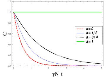
Figure 1: (Colour online) Coherence $C$ with respect to $\gamma Nt$
for the Werner state with $x=1$, with $a$ as a parameter. We have taken $a=0,1/2,3/4,1$ respectively. The red (large dashed) plot is for $a=0$, which is the usual Markovian case. The blue (thin line) plot is for $a=1/2$, while black (small dashed) and green (thick line) denote $a=3/4$ and $a=1$, respectively. The figure shows that with increment of $a$, the decay of coherence slows down and for the limiting case, it freezes after some time. The increment of coherence is the signature of the deviation from Markovian behavior.

In Fig.1, the evolution of $C_{l_{1}}$ with time (scaled by the decay parameter $\gamma$) is depicted. It can be seen that with the increment of the strength of the non-local environmental interaction, the decay of coherence slows down. For the limiting case of $a=1$, the $l_{1}$ norm of coherence is constant and equals to $C_{l_{1}}=x$. This limiting condition is attainable when the separation between the energy levels of both the atomic qubits is small. Whereas, for the local Markovian case we have $C_{l_{1}}=xe^{-2\gamma Nt}$. Hence it is clear, that the global part of the environmental interaction imposes a reverse flow of coherence into the system as opposed to the usual Markovian decay. Due to this reverse flow, the usual decoherence process slows down and may even stop, depending on the strength of the global interaction. The global interaction therefore generates a feedback to coherence at the expense of the population. In a recent work (frozen1, ), a dynamical condition has been proposed, under which the coherence of qubit systems is totally unaffected by noise. There the dynamical process under which the qubit system evolves is considered to be incoherent; that is, the process maps any incoherent state to the set of incoherent states. From the perspective of coherence resource theory, what we are claiming here is different from the motivation of that work. Here, we have taken a dynamical map, which acts as a resource for generating quantum coherence in a qubit system. For the low temperature case, we encounter a more interesting situation. Here the dynamics depends on the mixedness $x$ of the Werner state we have taken. For the initial pure state charectesized by $x=1$, the Coherence can be given by $C_{L1}^{Z}=e^{-(1-a)\gamma t}$. Hence, for the limiting case of $a=1$, the coherence is frozen at it’s initial maximum value 1. But for other cases ($x<1$), we have a finite contribution from the white noise part of the initial state, which makes the situation different.

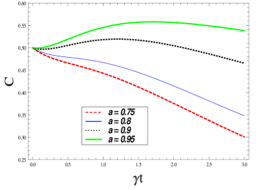
Figure 2: (Colour online) Coherence $C$ with respect to $\gamma t$
for the Werner state with $x=1/2$, with $a$ as a parameter. We have taken $a=0.75,0.8,0.9,0.95$ respectively. The figure shows that with increment of $a$, the decay of coherence slows down and as the global interaction increases, there is a generation of coherence.

From FIG. 2, we see that in the zero temperature regime, with the increase of global interaction, coherence not only stabilizes but also increase from it’s initial value, which shows a generation of coherence due to the global interaction.

Next, we will consider the dynamics of other quantum correlations like the entanglement and the Fisher information to further extend our study.

Let us now compare the dynamics of the coherence with that of the entanglement, expressed as the concurrence wotters ; hill . Entanglement is a very basic property of a composite quantum system, which gives rise to nontrivial phenomena in quantum information science. It is well known that many composite quantum systems having coherence (even some maximally coherent states) may not be entangled at all. For example, the maximally coherent state $|\psi\rangle=\frac{1}{2}(|00\rangle+|01\rangle+|10\rangle+|11\rangle)$ can be written in the form $|\psi\rangle=\frac{1}{\sqrt{2}}(|0\rangle+|1\rangle)\otimes\frac{1}{\sqrt{2}}(|0\rangle+|1\rangle)$, that is, the state is a product state and hence not entangled. This indicates that entanglement is a much more restricted quantum characteristic than coherence. We will now study the dynamics of concurrence for the global environmental interaction, to see whether it has a similar effect on entanglement as it had on coherence.

For any two qubit system, concurrence may be explicitly calculated from the density matrix as

$$E_{c}(\rho)=max\{0,\sqrt{\lambda_{1}}-\sqrt{\lambda_{2}}-\sqrt{\lambda_{3}}-\sqrt{\lambda_{4}}\},$$ (41)

where the quantities $\lambda_{i}$ (i=1,2,3,4) are the eigenvalues of the matrix (in decreasing order )

$$\tau=\rho(\sigma_{y}\otimes\sigma_{y})\rho^{*}(\sigma_{y}\otimes\sigma_{y}).$$ (42)

Here $\rho^{*}$ is the complex conjugate of the density matrix $\rho$ in the usual computational basis. For the X states we have taken in (21), the concurrence can be expressed in a simpler form as given by

$$E_{c}=2max\{0,(|\rho_{23}|-\sqrt{\rho_{11}\rho_{44}}),(|\rho_{14}|-\sqrt{\rho_{22}\rho_{33}})\}.$$ (43)

For the case of Werner states (38), the concurrence will be $E_{c}=2max\{0,|\rho_{23}|-\sqrt{\rho_{11}\rho_{44}}\}$. Hence, when $|\rho_{23}|>\sqrt{\rho_{11}\rho_{44}}$, the state is entangled. When the system is interacting with a hot bath, the expression of entanglement for Werner state is given by

$$\begin{array}[]{ll}E_{c}^{H}(\rho_{W})=\frac{x}{2}e^{-3\gamma Nt}\left[3\cosh\left(\gamma Nt\sqrt{1+8a^{2}}\right)+\left(\frac{6a-1}{\sqrt{1+8a^{2}}}\right)\sinh\left(\gamma Nt\sqrt{1+8a^{2}}\right)\right]-\frac{1}{2}.\end{array}$$ (44)

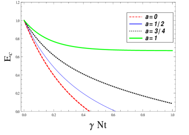
Figure 3: (Colour online) Concurrence $E_{C}$ versus $\gamma t$ for the Werner state with $x=1$, with $a$ as a parameter. We have taken $a=0,1/2,3/4,1$ respectively. The red (large dashed) plot is for $a=0$, which is the usual Markovian case. The blue (thin line) plot is for $a=1/2$, black (small dashed) plot is for $a=3/4$ and green (thick line) is for $a=1$. The figure shows that with increment of $a$, the sudden death of entanglement slows down, like a slow decay. For $a=1$, the sudden death vanishes completely and entanglement freezes to a particular value after a small initial decay.

From the Fig. 3, we see that entanglement decay also slows down with the increase in the strength of the global environmental interaction. For the limiting value $a=1$, after some initial decay, it also saturates like coherence. In this section, we have shown that the global system-bath interaction prolongs the lifetime of coherence and entanglement. With the increasing strength of the global part of the interaction (which is characterized by the parameter $a$ ), the lifetime of both the coherence and the entanglement increases.
Let us now consider the zero temperature situation. If we start from a maximally entangled state ($x=1$), we find that the entanglement can then be given by the expression $E(t)=e^{-(1-a)\gamma t}$. Which shows that entanglement decays exponentially. With the increase of the global interaction, the decay slows down and for the limiting case, it freezes. Similar to the case of coherence, here also the situation is a little different, when we start from an initial mixed state. Let us consider Werner state with $x=1/2$. In FIG. 4, we can see the evolution of entanglement with time. From the figure we can see that for zero temperature bath, there is a region of the evolution where entanglement is generated due to the global nature of the environmental interaction and it even surpasses the initial entanglement.

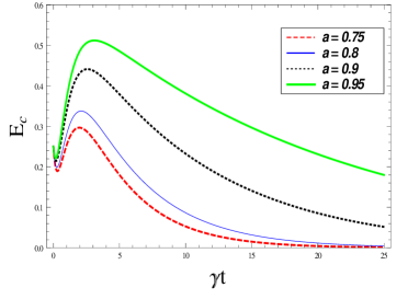
Figure 4: (Colour online) Concurrence $E_{C}$ versus $\gamma t$ for the Werner state with $x=1/2$, with $a$ as a parameter. We have taken $a=0.75,0.8,0.9,0.95$ respectively.

It is also important to note that not all states will show this behaviour of coherence and correlation freezing. For example, Werner states of the form $\frac{(1-x)}{4}\mathbb{I}+x|\psi^{+}\rangle\langle\psi^{+}|$ with $|\psi^{+}\rangle=(|00\rangle+|11\rangle)/\sqrt{2}$, will not show the above observed behavior of slowing down of coherence and correlation decay. This could be attributed to the form of the coherent part of the effective Hamiltonian (10) and (11), due to the global nature of the system-reservoir interaction. Following Ref. tanas , we can infer that under the evolution determined by the interaction Hamiltonian (11), the two atom system behaves as a single four level system with the ground state $|g\rangle$, the excited state $|e\rangle$ and two intermediate symmetric and anti-symmetric states $|s\rangle$ and $|as\rangle$, respectively. Where

$$\begin{array}[]{ll}|g\rangle=|00\rangle,~{}|e\rangle=|11\rangle,\\ |s\rangle=\frac{1}{\sqrt{2}}(|10\rangle+|01\rangle),\\ |as\rangle=\frac{1}{\sqrt{2}}(|10\rangle-|01\rangle).\end{array}$$ (45)

The Hamiltonian (10), which is generated by dipole-dipole interactions tanas , does not affect the ground and excited states. Only the symmetric and anti-symmetric states are affected by it. The incoherent part of the dipole-dipole interaction is basically the global part of the dynamical map with the strength $\gamma_{12}$. Therefore, the global interaction affects only $\rho_{23}$ and $\rho_{23}^{*}$, which are the components of the symmetric and anti-symmetric states. For the limiting case of $a=1$, the master equation can be written as

$$\begin{array}[]{ll}\frac{d\rho}{dt}=\frac{i}{\hbar}[\rho,H]\\ +\gamma(N+1)\left(J^{-}\rho J^{+}-\frac{1}{2}\left(J^{+}J^{-}\rho+\rho J^{+}J^{-}\right)\right)\\ +\gamma N\left(J^{+}\rho J^{-}-\frac{1}{2}\left(J^{-}J^{+}\rho+\rho J^{-}J^{+}\right)\right),\end{array}$$ (46)

with $J^{\pm}=\sigma^{\pm}_{1}+\sigma^{\pm}_{2}$. For this case the global interaction creates a decoherence free evolution for $\lvert s\rangle$ and $\lvert as\rangle$ and thus preserves the non-classicality of the states.

IV Generation of Quantumness and bound on Fisher information

In this section, we investigate the generation of non-classicality by the action of global bath in detail. We have considered a measure of quantumness and explicitely find it’s connection with quantum Fisher information and quantify the capacity of generation of “quantumness” of a global channel in detail. The Fisher information has considerable significance in statistical estimation theory, as a measure of “intrinsic accuracy” fisher . A quantum generalization of the Fisher information was proposed in Refs. helstrom and holevo . Here, we develop on the theme that the Fisher information can also be considered as a measure of non-classicality of a quantum system. It has been shown hall that the Fisher information of a quantum observable is proportional to the difference between quantum variance and the classical variance of the conjugate variable. The Fisher information of a parameterized family of probability densities $\{p_{\theta}:\theta\in\mathbb{R}\}$ on $\mathbb{R}$, is defined as

$$\begin{array}[]{ll}F(p_{\theta})=\\ \int_{\mathbb{R}}\left(\frac{\partial}{\partial\theta}p_{\theta}^{1/2}(x)\right)^{2}dx=\frac{1}{4}\int_{\mathbb{R}}\left(\frac{\partial}{\partial\theta}\log p_{\theta}^{1/2}(x)\right)^{2}p_{\theta}dx.\end{array}$$ (47)

Particularly, when $P_{\theta}(x)=p_{\theta}(x-\theta)$, then by translational invariance of the Lebesque integral, one can conclude that the Fisher information $F(p_{\theta})$ is independent of $\theta$. In that case the Fisher information can be denoted as $F(p)$ luo . A natural generalization of the Fisher information luo ; luo1 arises from (47), when we consider

$$\frac{\partial}{\partial\theta}p_{\theta}=\frac{1}{2}\left(\frac{\partial}{\partial\theta}\log p_{\theta}.p_{\theta}+p_{\theta}.\frac{\partial}{\partial\theta}\log p_{\theta}\right).$$ (48)

By replacing the integration by trace, probability $p_{\theta}$ by density matrix $\rho_{\theta}$ and the logarithmic derivative $\frac{\partial}{\partial\theta}\log p_{\theta}$ by the symmetric logarithmic derivative $L_{\theta}$, determined by

$$\frac{\partial}{\partial\theta}\rho_{\theta}=\frac{1}{2}(L_{\theta}\rho_{\theta}+\rho_{\theta}L_{\theta}),~{}~{}~{}~{}\theta\in\mathbb{R},$$ (49)

the Fisher information can be expressed as luo

$$F(p_{\theta})=\frac{1}{4}Tr(L_{\theta}^{2}\rho_{\theta}).$$ (50)

Now, if it is independent of the parameter $\theta$, it can be shown that $F(\rho,H)=\frac{1}{4}Tr(\rho L^{2})$ luo , where $i(\rho H-H\rho)=\frac{1}{2}(L\rho+\rho L)$. After some algebra, the Fisher information of an operator $H$ can be shown to be

$$F(\rho,H)=\frac{1}{2}\sum_{m,n}\frac{(\lambda_{m}-\lambda_{n})^{2}}{\lambda_{m}+\lambda_{n}}|\langle\psi_{m}|H|\psi_{n}\rangle|^{2},$$ (51)

where $\lambda_{m}$ and $|\psi_{m}\rangle$ are the eigenvalues and eigenvectors of the density matrix, respectively. It is to be noted that, if $H$ commutes with $\rho$, then the Fisher information $F(\rho,H)$ becomes zero. Hence, we will have non-zero Fisher information for an observable only when it is skewed or non-commuting with the density matrix. In Ref. hall , it was shown that, in the Schrödinger picture, the position Fisher information is equal to the square of the variance of the non-classical part of the conjugate momentum with a factor $4/\hbar^{2}$. This means that the Fisher information gives us a certain quantification of non-classicality or quantumness of a system. Hence the dynamics of Fisher information would be related to the dynamics of non-classicality associated with a quantum system.
Let us now elaborate the issue of “non-classicality” explicitely. In a recent work vedral , the notion of quantumness based on the non-commutivity of the algebra of observables has been investigated. A measure of quantumness has also been proposed based on the imcompatibility of quantum states. The mutual incompatibility of two given states $\rho_{a}$ and $\rho_{b}$ can be quantified by twice of the Hilbert-Schmidt norm of their commutator srikanth .

$$Q(\rho_{a},\rho_{b})=2\parallel[\rho_{a},\rho_{b}]\parallel^{2}=4Tr((\rho_{a}\rho_{b})^{2}-\rho_{a}^{2}\rho_{b}^{2})$$ (52)

We know that the trace of a positive operator is always positive and vanishes only when the operator is null. So $Q(\rho_{a},\rho_{b})$ is zero only when the the two density matrix commutes with each other. Given this fact, $Q(\rho_{a},\rho_{b})$ can be considered as a powerfull quantumness witness obeying the relation

$$0\leq Q(\rho_{a},\rho_{b})\leq 1$$ (53)

The intuitive understanding of $Q(\rho_{a},\rho_{b})$ as a measure of quantumness is clearly stated in Ref. vedral . Given an algebra $\mathbb{A}$ of the system observables, one can define the state $\rho$ to be classical if $Tr(\rho,[A,B])=0~{}~{}\forall A,B\in\mathbb{A}$, and the state is quantum otherwise. So the state is classical, if it does not detect the non-commutativity of the observables. Hence, intuitively it could be stated that if two states $\rho_{a}$ and $\rho_{b}$ do not commute, they are quantum and classical if otherwise. In Ref. vedral it has been shown that $Q(\rho_{a},\rho_{b})$ is proper witness of the global quantum nature of the given states. Now by chosing $\rho_{a}=\rho_{0}$ and $\rho_{b}=\rho_{t}$ as the initial and final state, we can quantify the generation of quantumness by a certain operation. If $\rho_{0}$ is a diagonal state in a given basis and the operation only alters the probability distribution, then the final state will also be a diagonal state. So then there will be no generation of non-commutativity and hence no generation of quantumness by the operation. For example, if we choose the initial state to be a incoherent state; i.e. the state is diagonal in the preffered basis and apply only incoherent operation, then the final state will also remain incoherent and no quantumness will be produced.
So let us take the initial state to be a diagonal state $\rho_{0}=\sum_{j=1}^{d}\lambda_{i}\lvert i\rangle\langle i\lvert$ and find the quantumness generated by any arbitrary process. Using Eq. (52), we find that

$$Q(\rho_{0},\rho_{t})=2\sum_{i\neq j}(\lambda_{i}-\lambda_{j})^{2}\lvert\langle i\lvert\rho_{t}\lvert j\rangle\lvert^{2}$$ (54)

Let us now quantify the quantum Fisher information generated by the process starting from a diagonal state. Using Eq. (51), we find that the generated Fisher information can be expressed as

$$F(\rho_{0},\rho_{t})=\frac{1}{2}\sum_{i\neq j}\frac{(\lambda_{i}-\lambda_{j})^{2}}{\lambda_{i}+\lambda_{j}}|\langle i|\rho_{t}\lvert j\rangle|^{2}.$$ (55)

Now we know that

$$\frac{1}{\lambda_{i}+\lambda_{j}}\geq 1~{}~{}~{}\forall~{}~{}i,j$$ (56)

and

$$|\langle i|\rho_{t}\lvert j\rangle|\leq 1~{}~{}~{}\forall~{}~{}i,j$$ (57)

Using Eq. (56) and (57), we find the following inequality

$$\frac{Q(\rho_{0},\rho_{t})}{4}\leq F(\rho_{0},\rho_{t})\leq\frac{C_{l_{1}}(\rho_{0},\rho_{t})}{2}.$$ (58)

The relation gives us the intuitive insight on the nature of quantum Fisher information as a measure of quantumness. The left equality of (58) will strictly hold for two level system, which is the smallest possible quantum system. For higher dimensional systems and systems consisting more than one party, the situation gets much more complicated. Because for composite system, quantum correlation comes into picture. From (58), we also surmise that the created coherence is always more than the created Fisher information.
Let us now calculate the quantumness and Fisher information generated by our specific global operation. Here we will consider an initial diagonal state of the form

$$\rho_{0}=\left(\begin{matrix}\rho_{11}(0)&0&0&0\\ 0&\rho_{22}(0)&0&0\\ 0&0&\rho_{33}(0)&0\\ 0&0&0&\rho_{44}(0)\end{matrix}\right)$$ (59)

The generated quantumness and Fisher information by the action of our global operation can thus be respectively expressed as

$$Q(\rho_{0},\rho_{t})=(\rho_{22}(0)-\rho_{33}(0))^{2}C^{2}(\rho_{0},\rho_{t})$$ (60)

$$F(\rho_{0},\rho_{t})=\frac{(\rho_{22}(0)-\rho_{33}(0))^{2}}{\rho_{22}(0)+\rho_{33}(0)}\frac{C^{2}(\rho_{0},\rho_{t})}{4}$$ (61)

where $C(\rho_{0},\rho_{t})=2\lvert\rho_{23}(t)\lvert$ is the generated coherence. For the case of global environmental interaction, we find the inequality

$$\frac{Q(\rho_{0},\rho_{t})}{4}\leq F(\rho_{0},\rho_{t})\leq\frac{C^{2}(\rho_{0},\rho_{t})}{4}.$$ (62)

Since $0\leq C(\rho_{0},\rho_{t})\leq 1$, we find that the created coherence will always be greater than the created Fisher information and quantumness.

For the hot bath, we find the quantumness produced from a diagonal state can be expressed as

$$Q(\rho_{0},\rho_{t})=16U^{\prime 2}(0)e^{-6\gamma Nt}\left[\frac{4a^{2}}{1+8a^{2}}(U(0)-W(0))^{2}\sinh^{2}\left(\gamma Nt\sqrt{1+8a^{2}}\right)+U^{\prime 2}(0)e^{2\gamma Nt}\sin^{2}(2\Omega_{12}t)\right]$$ (63)

The generated quantum Fisher information can be expressed as

$$F(\rho_{0},\rho_{t})=\frac{Q(\rho_{0},\rho_{t})}{8U(0)}$$ (64)

So we see that the generated Fisher information is equal to the generated quantumness with a factor $1/8U(0)$. Let us consider a particular case with $\rho_{11}(0)=\rho_{44}(0)=0$, $\rho_{22}(0)=3/4$ and $\rho_{33}(0)=1/4$. For this case $F(\rho_{0},\rho_{t})=Q(\rho_{0},\rho_{t})/4$. Now in the case of high temperature bath ($N>>1$), the contribution from the unitary evolution will not play a significant role.

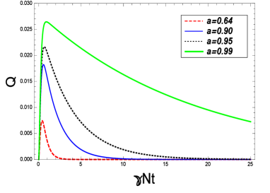
Figure 5: (Colour online) Generated Quantumness $Q$ as a function of $\gamma Nt$. We have taken the global interaction parameter $a=0.64,0.90,0.95,0.99$ respectively. Corresponding to each value of $a$, we have $b=0,-0.45,-0.78,-1.84$ respectively. But for the High temperature case as presented in this plot, the effect of $b$, which is due to the unitary evolution is very small

From FIG. 5, we see the generation of quantumness with increasing global interaction. In FIG. 6 we see the generation of coherence with increasing global interaction. The strength of the unitary interaction is characterized by $\Omega_{12}$ given by equation (12). For the rest of the numerical study, we parametrize $b=\Omega_{12}/\gamma$.

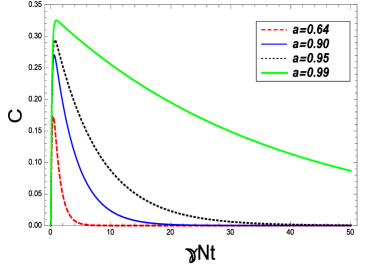
Figure 6: (Colour online) Generated Coherence $C$ as a function of $\gamma Nt$. We have taken the global interaction parameter $a=0.64,0.90,0.95,0.99$ respectively. Corresponding to each value of $a$, we have $b=0,-0.45,-0.78,-1.84$ respectively.

But for the high temperature case, no generation of entanglement is observed.
It is important to state that in this case of high temperature bath, the role of the unitary evolution in generating quantumness is not prominant, because it is suppressed by the much stronger non-unitary dynamics of the qubit-bath interaction. Whereas in the Zero temperature bath we see a different picture.

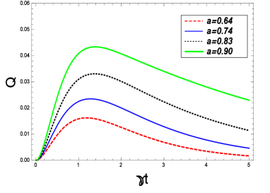
Figure 7: (Colour online) Generated Quantumness $Q$ for zero temperature bath case as a function of $\gamma t$. We have taken the global interaction parameter $a=0.64,0.74,0.83,0.90$ respectively. Corresponding to each value of $a$, we have $b=0,-0.10,-0.24,-0.45$ respectively.

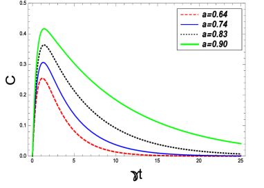
Figure 8: (Colour online) Generated Coherence $C$ for zero temperature bath case as a function of $\gamma t$. We have taken the global interaction parameter $a=0.64,0.74,0.83,0.90$ respectively. Corresponding to each value of $a$, we have $b=0,-0.10,-0.24,-0.45$ respectively.

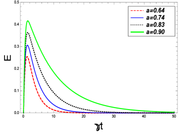
Figure 9: (Colour online) Generated Entanglement $E$ for zero temperature bath case as a function of $\gamma t$. We have taken the global interaction parameter $a=0.64,0.74,0.83,0.90$ respectively. Corresponding to each value of $a$, we have $b=0,-0.10,-0.24,-0.45$ respectively.

From FIG.7 and FIG.8, we see the generation of quantumness and coherence in zero temperature bath, starting from a initial diagonal state. Importantly, for zero temperature global bath, we can also see a generation of entanglement from FIG. 9, which is unlike the case of high temperature bath.

V Global master equation with time varying parameters

In this section, we further generalize our global master equation by considering the memory effect of the bath. In a practical situation, an environment usually has memory. In an experiment, a composite quantum system can be exposed to various kind of noises such as vacuum noise, phase noise, thermal noise as well as a mixture of different kind of noises. Different noise models has been proposed in recent years to model solvable approximate master equations Zyczkowski ; Daffer . Correlation dynamics in the Markovian (no memory) regime has been extensively studied sbindranil . However, in practice, an environment is more likely to be non-Markovian. A systematic investigation of the dynamics of quantum coherence and correlation in the presence of non-Markovian noise is an ongoing study yu ; kubo . Here we are going to analyze the time dependent global environmental operation based on a non-markovian model of quantum state diffusion gisin . For certain cases, the Lindblad type master equation can be constructed from non-linear stochastic Schrödinger equation of the form

$$\frac{d}{dt}\psi_{t}=-iH\psi_{t}+L\psi_{t}\circ z_{t}-\frac{1}{2}L^{\dagger}\int_{0}^{t}\alpha(t,s)\frac{\delta\psi_{t}}{\delta z_{t}}ds.$$ (65)

where $z_{t}$ is a white complex valued Wiener process: $z_{t}=\sum_{\nu}z_{\nu}e^{i\nu t}$. The correlation relations are defined as

$$M[z_{t}^{*}z_{s}]=\delta(t-s)~{}~{};~{}~{}M[z_{t}z_{s}]=0,$$ (66)

and $\alpha(t,s)$ is the environmental correlation function. Here $M[\cdots]$ is the ensemble mean over the classical noise $z_{t}$ and the system density matrix $\rho_{t}=M[\lvert\psi(t)\rangle\langle\psi(t)\lvert]$. The system Hamiltonian is taken to be $H=\frac{\omega}{2}\sigma_{z}$. The stochastic environmental influence is expressed by the gaussian Wiener process $Z_{t}$, which drives the system through the operator $L$. For our case of dissipative process described by amplitude damping operation, $L$ is chosen as $\lambda\sigma_{-}$. Here $\lambda$ is a parameter describing the strength of interaction. Now for dissipative interactions, one can choose

$$\frac{\delta\psi_{t}}{\delta z_{t}}=f(t,s)\sigma_{-}\psi_{t},$$ (67)

where $f(t,s)$ is a function to be determined. For the dynamics to be physically consistant this function satisfies the relation gisin

$$\partial_{t}f(t,s)=[i\omega+\lambda F(t)]f(s,t),$$ (68)

with the initial condition $f(s,s)=\lambda$. Here $F(t)=\int_{0}^{t}\alpha(t,s)f(t,s)ds$. Assuming exponentially decaying environmental correlation $\alpha(t,s)=\frac{\gamma_{0}}{2}\exp\left(-\gamma_{0}\lvert t-s\lvert+i\xi(t-s)\right)$, we find the reduced map for the system to be

$$\left(\begin{matrix}\rho_{11}(0)e^{-\int_{0}^{t}(F(s)+F^{*}(s))ds}&\rho_{12}(0)e^{-i\omega t-\int_{0}^{t}F(s)ds}\\ \rho_{21}(0)e^{i\omega t-\int_{0}^{t}F^{*}(s)ds}&1-\rho_{11}(t)\end{matrix}\right)$$ (69)

with

$$\begin{array}[]{ll}F(t)=\frac{\gamma_{0}}{2\lambda}-\frac{\sqrt{\gamma_{0}^{2}-2\gamma_{0}\lambda^{2}}}{2\lambda}\\ ~{}~{}~{}~{}~{}~{}~{}~{}\times\tanh\left[\frac{t}{2}\sqrt{\gamma_{0}^{2}-2\gamma_{0}\lambda^{2}}+\tanh^{-1}\left(\frac{\gamma_{0}}{\sqrt{\gamma_{0}^{2}-2\gamma_{0}\lambda^{2}}}\right)\right].\end{array}$$ (70)

Here the resonant situation $\omega=\xi$ is considered. Here two different cases can be considered. The first one is short memory or weak coupling with $\gamma>2\lambda^{2}$. The much more interesting situation appears for long memory or strong coulping case where we have $\gamma<2\lambda^{2}$. Then we have

$$\begin{array}[]{ll}F(t)=\frac{\gamma_{0}}{2\lambda}+\frac{\sqrt{2\gamma_{0}\lambda^{2}-\gamma_{0}^{2}}}{2\lambda}\\ ~{}~{}~{}~{}~{}~{}~{}~{}\times\tan\left[\frac{t}{2}\sqrt{2\gamma_{0}\lambda^{2}-\gamma_{0}^{2}}-\tan^{-1}\left(\frac{\gamma_{0}}{\sqrt{2\gamma_{0}\lambda^{2}-\gamma_{0}^{2}}}\right)\right].\end{array}$$ (71)

The master equation of the mentioned operation can be derived from the map given in Eq. (69) with the form

$$\dot{\rho}=i\frac{\omega}{2}[\sigma_{Z},\rho]+\lambda[F(t)+F^{*}(t)]\left(\sigma^{-}\rho\sigma^{+}-\frac{1}{2}\{\sigma^{+}\sigma^{-},\rho\}\right)$$ (72)

Note that, here only the zero temperature situation is considered for simplicity. So there is only the dissipation part, but no reheating. But it can always be generalized for a finite temperature bath. Now for a two qubit system with identical qubits, where the bath acting globally, we can generalize the master equation as

$$\begin{array}[]{ll}\frac{d\rho}{dt}=-\frac{i}{\hbar}[\rho,H_{S}(t)]+\sum_{i,j}\gamma_{ij}(t)\left(\sigma_{i}^{-}\rho\sigma_{j}^{+}-\frac{1}{2}\{\sigma_{i}^{+}\sigma_{j}^{-},\rho\}\right),\end{array}$$ (73)

with

$$H_{S}(t)=\sum_{i=1,2}\left(\frac{1}{2}\hbar\sigma_{Z}^{i}+\hbar\Omega_{ij}(t)\left(\sigma_{i}^{-}\sigma_{j}^{+}+\sigma_{i}^{+}\sigma_{j}^{-}\right)\right)$$ (74)

and

$$\begin{array}[]{ll}\Omega_{12}=\frac{3}{4}\gamma(t)b(k_{0}r_{12})\\ \gamma_{12}=\frac{3}{2}\gamma(t)a(k_{0}r_{12})\\ \gamma(t)=\lambda[F(t)+F^{*}(t)]\end{array}$$ (75)

The solution of Eq. (73) takes the form

$$\begin{array}[]{ll}\rho_{11}(t)=\rho_{11}(0)e^{-2G(t)},\\ \rho_{22}(t)=U_{n}(t)+U_{n}(^{\prime}t),\\ \rho_{33}(t)=U_{n}(t)-U^{\prime}_{n}(t),\\ \rho_{44}(t)=1-\rho_{11}(t)-2U_{n}(t),\\ \rho_{23}=V_{n}(t)+iV^{\prime}_{n}(t),\\ \rho_{14}(t)=\rho_{14}(0)\exp\left(-G(t)\right).\end{array}$$ (76)

where

$$\begin{array}[]{ll}U_{n}(t)=U_{n}(0)e^{-G(t)}\cosh(aG(t))-V_{n}(0)e^{-(G(t))}\sinh(aG(t))\\ +\frac{\rho_{11}(0)}{2}\left[\frac{1+a}{1-a}e^{-(1+a)G(t)}\left(1-e^{-(1-a)G(t)}\right)+\frac{1-a}{1+a}e^{-(1-a)G(t)}\left(1-e^{-(1+a)G(t)}\right)\right],\end{array}$$ (77)

$$\begin{array}[]{ll}V_{n}(t)=V_{n}(0)e^{-G(t)}\cosh(aG(t))-U_{n}(0)e^{-G(t)}\sinh(aG(t))\\ +\frac{\rho_{11}(0)}{2}\left[\frac{1+a}{1-a}e^{-(1+a)G(t)}\left(1-e^{-(1-a)G(t)}\right)-\frac{1-a}{1+a}e^{-(1-a)G(t)}\left(1-e^{-(1+a)G(t)}\right)\right],\end{array}$$ (78)

$$\begin{array}[]{ll}U^{\prime}_{n}(t)=U^{\prime}_{n}(0)e^{-G(t)}\cosh(2bG(t))-V^{\prime}_{n}(0)e^{-G(t)}\sinh(2bG(t))\end{array}$$ (79)

$$\begin{array}[]{ll}V^{\prime}_{n}(t)=V^{\prime}_{n}(0)e^{-G(t)}\cosh(2bG(t))-U^{\prime}_{n}(0)e^{-G(t)}\sinh(2bG(t))\end{array}$$ (80)

where

$$G(t)=\gamma_{0}t-2\ln\left[\sqrt{\frac{2\gamma_{0}\lambda^{2}}{2\gamma_{0}\lambda^{2}-\gamma_{0}^{2}}}\left\lvert\cos\left(\frac{t}{2}\sqrt{2\gamma_{0}\lambda^{2}-\gamma_{0}^{2}}-\tan^{-1}\left(\frac{\gamma_{0}}{\sqrt{2\gamma_{0}\lambda^{2}-\gamma_{0}^{2}}}\right)\right)\right\lvert\right]$$ (81)

V.1 Dynamics of coherence and entanglement for Werner state

In this subsection, we are analysing the dynamics of coherence and concurrence for two qubit Werner state as mentioned in Eq. (38). For a initial pure state ($x=1$), the coherence dynamics is given by $C(\rho_{W})=e^{-(1-a)G(t)}$. From FIG. 10 we see that global environmental interaction helps the backflow of information process and as a consequence we see a periodic revival of coherence with increasing global interaction.

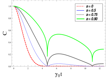
Figure 10: (Colour online) Dynamics of coherence $C$ for Werner state with $x=1$ interacting with a zero temperature global non-markovian bath case as a function of $\gamma_{0}t$. We have taken the global interaction parameter $a=0,0.5,0.75,0.90$ respectively. Here we have taken $\lambda^{2}=\gamma_{0}$.

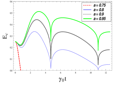
Figure 11: (Colour online) Dynamics of entanglement $E_{c}$ for Werner state with $x=1/2$ interacting with a zero temperature global non-markovian bath case as a function of $\gamma_{0}t$. We have taken the global interaction parameter $a=0,0.5,0.75,0.90$ respectively. Here we have taken $\lambda^{2}=\gamma_{0}$.

For entanglement also, we see that the global environmental interaction helps the periodic revival of entanglement, as shown in FIG. 11.

V.2 Generation of Quantumness

Here we analyse the generation of quantumness by global non-marokivan interaction. Here also we see that global interaction enhances the generation of non-classicality.

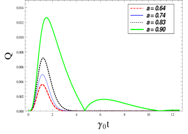
Figure 12: (Colour online) Generated Quantumness $Q$ for zero temperature bath case as a function of $\gamma t$. We have taken the global interaction parameter $a=0.64,0.74,0.83,0.90$ respectively. Corresponding to each value of $a$, we have $b=\Omega_{12}/2\gamma=0,-0.10,-0.24,-0.45$ respectively.

VI Conclusion

To conclude, in this work we exploit a useful global system-environment interaction and study the effect of non-Markovian behaviour on various facets of quantum coherence and correlations. Here we have found that the global part of the environmental interaction is acting as a resource to compensate the decoherence effect. We have further extended our result to the case where the bath has memory. We have given the exact solution of the proposed master equation for two separate cases of high temperature and zero temperature bath for the memoryless case. For the case for environmental interaction in presence of memory, we have given exact solution for the zero temperature bath. But it can be easily extended to the case of finite temperature bath as well. We have shown that with increasing strength of the global part of the environmental interaction, both coherence and entanglement decay slows down and for the limiting case they eventually freeze. The limiting condition is attainable when the separation between the energy levels of both the atomic qubits is small. For the memory dependent non-Markovian case, we have seen that the global interaction enhances the regeneration of coherence, entanglement and quantumness. Which tells us that the global interaction helps the backflow of information from environment to the system via non-Markovian interaction. It is also very important to mention here that for the case of zero temperature bath, as the strength of the global interaction increases, the unitary interaction between the two qubits will dominate. In that case, the limiting condition is unattainable. Because then the environment cannot resolve the two interacting qubits. Instead it sees the system as a single four level level system in the eigenbasis of it’s total Hamiltonian. Moreover, we have also quantified the amount of non-classicality generated by global environmental interaction. It has been shown that the generated quantum Fisher information is lower bounded by the Quantumness with a factor of $1/4$ and upper bounded by the $l_{1}$ norm of coherence with a factor of 1/2. This gives us an intuitive understanding of quantum Fisher information as a measure of non-classicality. Fisher information and the quantumness measure are both based on the non-commutativity of states and this property is precisely understood as the non-classicality of quantum states. Now from the inequality relation given by Eq. (58), we find that the created coherence by any arbitrary global operation is always greater than the created quantumness and Fisher information. So we understand that coherence contains more than the non-classicality of quantum states and hence cannot be considered as a proper measure of Quantumness. To summarize, in this work we have examined the emergence of non-Markovianity and its impact on the evolution of a number of facets of quantumness in the system. It is observed that non-Markovianity can play a nontrivial and useful role in various quantum information tasks where coherence and entanglement are considered as resources.

References

- (1) H. P. Breuer and F. Petruccione, The Theory of Open Quantum Systems, (Oxford University Press, Oxford, 2007).
- (2) U. Weiss, Quantum Dissipative Systems, (World Scientific,Singapore, 2000).
- (3) X. S. Ma et. al.,Quantum teleportation over 143 kilometres using active feed-forward, Nature 489, 269-273 (2012).
- (4) J.I. Cirac, P. Zoller, J.H. Kimble, et al., Quantum State Transfer and Entanglement Distribution among Distant Nodes in a Quantum Network, Phys. Rev. Lett, 78, 3221-3224 (1997).
- (5) D. Bouwmeester, J.W. Pan, K. Mattle et al., Experimental quantum teleportation, Nature, 390, 575-579 (1997).
- (6) M. A. Nielsen and I. L. Chuang, Quantum Computation and Quantum Information, (Cambridge Univ. Press,Cambridge, 2000).
- (7) Y. C. Liang, D. Kaszlikowski, B.-G. Englert, L. C. Kwek, and C. H. Oh, Tomographic quantum cryptography, Phys. Rev. A 68, 022324 (1-9) (2003).
- (8) S. Banerjee and R. Srikanth, Eur. Phys. J. D 46,Geometric phase of a qubit interacting with a squeezed-thermal bath, 335-344 (2008); S. N. Sandhya and S. Banerjee,Geometric phase: an indicator of entanglement, Euro. Phys. J. D: 66, 168 (1-6) (2012); S. Banerjee, C. M. Chandrashekar and A. K. Pati,Enhancement of geometric phase by frustration of decoherence: A Parrondo-like effect, Phys. Rev. A 87, 042119 (1-5) (2013).
- (9) R. Srikanth and S. Banerjee, Squeezed generalized amplitude damping channel, Phys. Rev. A 77, 012318 (1-9) (2008).
- (10) C. M. Chandrashekar, R. Srikanth and S. Banerjee, Symmetries and noise in quantum walk, Phys. Rev. A 76, 022316 (1-15) (2007); S. Banerjee, R. Srikanth, C. M. Chandrashekar and Pranaw Rungta, Symmetry-noise interplay in a quantum walk on an n-cycle, Phys. Rev. A 78, 052316 (1-5) (2008); R. Srikanth, S. Banerjee and C. M. Chandrashekar, Quantumness in a decoherent quantum walk using measurement-induced disturbance, Phys. Rev. A 81, 062123 (1-7) (2010).
- (11) K. Thapliyal, S. Banerjee, A. Pathak, S. Omkar and V. Ravishankar, Quasiprobability distributions in open quantum systems: Spin-qubit systems, Ann. of Phys. 362, 261-286 (2015).
- (12) K. Thapliyal, S. Banerjee and A. Pathak, Tomograms for open quantum systems: In(finite) dimensional optical and spin systems, Ann. of Phys. 366, 148-167 (2016).
- (13) S. Goyal, S. Banerjee and S. Ghosh, Effect of control procedures on the evolution of entanglement in open quantum systems, Phys. Rev. A: 85, 012327 (1-17) (2012).
- (14) S. Banerjee and R. Ghosh, Quantum theory of a Stern-Gerlach system in contact with a linearly dissipative environment, Phys. Rev. A 62, 042105 (1-8) (2000).
- (15) S. Banerjee and R. Ghosh, General quantum Brownian motion with initially correlated and nonlinearly coupled environment, Phys. Rev. E. 67, 056120 (1-13) (2003).
- (16) A. Ishizaki and G. R. Fleming, On the adequacy of the Redfield equation and related approaches to the study of quantum dynamics in electronic energy transfer, J. Chem. Phys. 130, 234110 (1-8) (2009).
- (17) B. Leggio, R. Lo Franco, D. O. Soares-Pinto, P. Horodecki, and G. Compagno, Distributed correlations and information flows within a hybrid multipartite quantum-classical system, Phys. Rev. A 92, 032311 (1-8) (2015).
- (18) Z.-X. Man, Y.-J. Xia, and R. Lo Franco, Cavity-based architecture to preserve quantum coherence and entanglement, Sci. Rep. 5, 13843 (1-13) (2015).
- (19) J.-S. Xu, K. Sun, C.-F. Li, X.-Y. Xu, G.-C. Guo, E. Andersson, R. Lo Franco and G. Compagno,Experimental recovery of quantum correlations in absence of system-environment back-action, Nat. Commun. 4, 2851 (1-7)(2013).
- (20) R. Lo Franco, B. Bellomo, S. Maniscalco, and G. Compagno, Dynamics of quantum correlations in two qubit systems within non-Markovian environments, Int. J. Mod. Phys. B 27, 1345053 (1-20) (2013).
- (21) Z.-X. Man, Y.-J. Xia, and R. Lo Franco, Harnessing non-Markovian quantum memory by environmental coupling, Phys. Rev. A 92, 012315 (1-8) (2015).
- (22) M. M. Wolf et. al., Assessing Non-Markovian Quantum Dynamics, Phys. Rev. Lett. 101, 150402 (1-4) (2008).
- (23) H.P. Breuer et. al., Measure for the Degree of Non-Markovian Behavior of Quantum Processes in Open Systems, Phys. Rev. Lett. 103, 210401 (1-4) (2009).
- (24) E.M. Laine et. al., Measure for the non-Markovianity of quantum processes, Phys. Rev. A 81, 062115 (1-8) (2010).
- (25) A. Rivas et. al., Entanglement and Non-Markovianity of Quantum Evolutions, Phys. Rev. Lett. 105, 050403 (1-4) (2010).
- (26) A. K. Rajagopal, A. R. Usha Devi and R. W. Rendell, Kraus representation of quantum evolution and fidelity as manifestations of Markovian and non-Markovian forms, Phys. Rev. A 82, 042107 (1-7) (2010).
- (27) H. P. Breuer, Foundations and measures of quantum non-Markovianity, J. Phys. B: At. Mol. Opt. Phys. 45, 154001 (1-12) (2012).
- (28) Kishore Thapliyal, Anirban Pathak and Subhashish Banerjee, Quantum cryptography over non-Markovian channels, Quantum Inf Process 16, 115 (1-21) (2017).
- (29) Subhashish Banerjee, N. Pradeep Kumar, R. Srikanth, Vinayak Jagadish, Francesco Petruccione, Non-Markovian Dynamics of Discrete-Time Quantum Walks, arXiv:1703.08004 (2017).
- (30) Pradeep Kumar, Subhashish Banerjee, R. Srikanth, Vinayak Jagadish, Francesco Petruccione, Non-Markovian evolution: a quantum walk perspective, arXiv:1711.03267 (2017).
- (31) T. Baumgratz, M. Cramer, and M. B. Plenio, Quantifying Coherence, Phys. Rev. Lett. 113, 140401 (1-5) (2014).
- (32) A. Winter and D. Yang, Operational Resource Theory of Coherence, Phys. Rev. Lett. 116, 120404 (1-6) (2016).
- (33) A. Streltsov, U. Singh, H. S. Dhar, M. N. Bera and G. Adesso, Measuring Quantum Coherence with Entanglement, Phys. Rev. Lett. 115, 020403 (1-6) (2015).
- (34) U. Singh, M. N. Bera, H. S. Dhar, and A. K. Pati, Maximally coherent mixed states: Complementarity between maximal coherence and mixedness, Phys. Rev. A 91 052115 (1-8) (2015).
- (35) U. Singh, M.N. Bera, A. Misra and A.K. Pati, Erasing Quantum Coherence: An Operational Approach, arXiv:1506.08186 (2015).
- (36) E. Chitambar, A. Streltsov, S. Rana, M. N. Bera, G. Adesso and M. Lewenstein, Assisted Distillation of Quantum Coherence, Phys. Rev. Lett. 116 070402 (1-5) (2016).
- (37) S. Rana, P. Parashar and M. Lewenstein, Trace-distance measure of coherence, Phys. Rev. A 93 012110 (1-7) (2016).
- (38) JI de Vicente and A. Streltsov, Genuine quantum coherence, J. Phys. A: Math. Theor. 50 045301 (1-35) (2017) .
- (39) T. Chanda and S. Bhattacharya,Delineating incoherent non-Markovian dynamics using quantum coherence, Annals of Physics 366, 1-12 (2016).
- (40) N. Tang, W. Cheng and H-S. Zeng, Coherence, correlation and non-Markovianity in qubit systems, Eur. Phys. J. D 68, 278 (1-8) (2014).
- (41) S. Banerjee, V. Ravishankar and R. Srikanth, Dynamics of entanglement in Two-Qubit Open System Interacting with a Squeezed Thermal Bath via Dissipative interaction, Annals of Physics 325, 816-834 (2010).
- (42) Z. Ficek and R. Tanas, Entangled states and collective nonclassical effects in two-atom systems, Physics Reports 372, 369-443 (2002).
- (43) R. A. Fisher, Theory of Statistical Estimation, Proc. Cambridge Philos. Soc. 22, 700-725 (1925).
- (44) C. R. Rao, Information and accuracy attainable in the estimation of statistical parameters, Bulletin of the Calcutta Mathematical Society 37, 81-91 (1945).
- (45) C. W. Helstrom, Quantum Detection and Estimation Theory, (Academic Press, New York, 1976).
- (46) A. S. Holevo, Probabilistic and Statistical Aspects of Quantum Theory, (North-Holland, Amsterdam, 1982), Chapter VI.
- (47) M. J. W. Hall, Quantum properties of classical Fisher information, Phys. Rev. A 62 012107 (1-6), (2000).
- (48) S. Banerjee, A. K. Alok and S. Omkar, Quantum Fisher and skew information for Unruh accelerated Dirac qubit, Eur. Phys. J. C 76, 437 (1-9) (2016).
- (49) Leonardo Ferro, Paolo Facchi, Rosario Fazio, Fabrizio Illuminati, Giuseppe Marmo, Vlatko Vedral and Saverio Pascazio, Measuring quantumness: from theory to observability in interferometric setups, arXiv: 1501.03099v1 (2015).
- (50) P.Iyengar, G.N.Chandan and R. Srikanth, Quantifying quantumness via commutators: an application to quantum walk, arXiv:1312.1329 (2013).
- (51) J. Preskill, Quantum Information and Computation, Lecture Notes for Physics Vol. 229 (Springer, Berlin, 1998).
- (52) D. A. Lider et.al., Condensed Matter From Completely Positive Maps to the Quantum Markovian Semigroup Master Equation, Chem. Phys. 268, 35-53 (2001).
- (53) T. Yu and J. H. Eberly, Evolution from Entanglement to Decoherence of Bipartite Mixed ”X” States, Quantum Inform. Comput. 7, 459-468 (2007).
- (54) A. R. P. Rau, Algebraic characterization of X-states in quantum information, J. Phys. A 42, 412002 (1-7) (2009).
- (55) R. J. Glauber, Coherent and Incoherent States of the Radiation Field, Phys. Rev. 131, 2766 (1-23) (1963).
- (56) E. C. G. Sudarshan, Equivalence of Semiclassical and Quantum Mechanical Descriptions of Statistical Light Beams, Phys. Rev. Lett. 10, 277 (1-3) (1963).
- (57) J. Almeida, P. C. de Groot, S. F. Huelga, A. M. Liguori, and M. B. Plenio,Probing quantum coherence in qubit arrays, J. Phys. B: At. Mol.Opt. Phys. 46, 104002 (1-8) (2013).
- (58) S. Lloyd, Quantum coherence in biological systems, J. Phys.: Conf. Ser. 302, 012037 (1-5) (2011).
- (59) E. Romero, R. Augulis, V. I. Novoderezhkin, M. Ferretti, J. Thieme, D. Zigmantas, and R. V. Grondelle, Quantum Coherence in Photosynthesis for Efficient Solar Energy Conversion, Nature Phys. 10, 676-682 (2014).
- (60) P. Rebentrost, M. Mohseni, I. Kassal, S. Lloyd, and A. Aspuru-Guzik, Environment-assisted quantum transport, New Journal of Physics 11, 033003 (1-13) (2009).
- (61) D. Manzano, M. Tiersch, A. Asadian, and H. J. Briegel, Quantum transport efficiency and Fourier’s law Physical Review E 86, 061118 (1-5) (2012).
- (62) D. Kondepudi and I. Prigogine, Modern Thermodynamics (John Wiley and Sons Ltd, Sussex, England, 1998).
- (63) H. Spohn, Entropy production for quantum dynamical semigroups, Journal of Mathematical Physics 19, 1227 (1-5)(1978).
- (64) F. G. S. L. Brandao, N. H. Y. Ng, J. Oppenheim, and S. Wehner, The second laws of quantum thermodynamics, PNAS 112, 3275-3279 (2015).
- (65) M. Scully, M. Zubairy, G. S. Agarwal, and H. Walther, Extracting Work from a Single Heat Bath via Vanishing Quantum Coherence, Science 299, 862-864 (2003).
- (66) M. O. Scully, Quantum Photocell: Using Quantum Coherence to Reduce Radiative Recombination and Increase Efficiency, Physical Review Letters 104, 207701 (1-4) (2010).
- (67) M. Mohseni, P. Rebentrost, S. Lloyd, and A. AspuruGuzik, Environment-assisted quantum walks in photosynthetic energy transfer, The Journal of Chemical Physics 129, 174106 (1-10)(2008).
- (68) M. B. Plenio and S. F. Huelga, Dephasing-assisted transport: quantum networks and biomolecules New Journal of Physics 10, 113019 (1-15) (2008).
- (69) P. Rebentrost, M. Mohseni, I. Kassal, S. Lloyd, and A. Aspuru-Guzik, Environment-assisted quantum transport New Journal of Physics 11, 033003 (1-13) (2009).
- (70) D. Manzano, M. Tiersch, A. Asadian, and H. J. Briegel, Quantum transport efficiency and Fourier’s law, Phys. Rev. E 86, 061118 (1-5) (2012).
- (71) Y. L. Lin et.al., Dissipative production of a maximally entangled steady state, Nature 504, 415418 (2013); G.P. Beretta, Maximum entropy production rate in quantum thermodynamics, J. Phys.: Conf. Ser. 237, 012004 (1-32) (2010); A. Mari and J. Eisert, Cooling by Heating: Very Hot Thermal Light Can Significantly Cool Quantum Systems, PRL 108, 120602 (1-5) (2012); Luis A. Correa et.al., Quantum-enhanced absorption refrigerators, Scientific Reports 4, 3949 (1-9) (2014).
- (72) M.N. Bera, T. Qureshi, M.A. Siddiqui, A.K. Pati, Duality of quantum coherence and path distinguishability, Phys. Rev. A 92, 012118 (1-6) (2015).
- (73) A. K. Alok, S. Banerjee and S. U. Sankar, Quantum correlations in terms of neutrino oscillation probabilities, arXiv:1411.5536 (2014).
- (74) T. R. Bromley, M. Cianciaruso, and G. Adesso, Frozen Quantum Coherence, Phys. Rev. Lett. 114, 210401 (1-6) (2015).
- (75) W. K. Wootters, Entanglement of Formation of an Arbitrary State of Two Qubits, Phys. Rev. Lett. 80, 2245 (1-4) (1998).
- (76) S. Hill and W. K. Wootters, Entanglement of a Pair of Quantum Bits, Phys. Rev. Lett. 78, 5022 (1-4) (1997).
- (77) S. Luo, Wigner-Yanase skew information vs. quantum Fisher information, Proc. of Am. Math. Soc. 132, 885-890 (2003).
- (78) S. Luo, Wigner-Yanase Skew Information and Uncertainty Relations, Phys. Rev. Lett. 91, 180403 (1-4) (2003); S. Luo and Q. Zhang, Informational distance on quantum-state space , Phys. Rev. A 69, 032106 (1-8) (2004).
- (79) K. Zyczkowski et al., Dynamics of quantum entanglement, Phys. Rev. A 65, 012101 (1-9) (2001).
- (80) S. Daffer, K. Wodkiewicz and J. K. McIver, Quantum Markov channels for qubits, Phys. Rev. A 67, 062312 (1-13) (2003).
- (81) I. Chakrabarty, S. Banerjee and N. Siddharth, A study of Quantum Correlations in Open Quantum Systems, Quantum Information and Computation 11, 0541-0562 (2011).
- (82) T. Yu and J. H. Eberly, Entanglement Evolution in a Non-Markovian Environment, Optics Communications 283, 676-680 (2010).
- (83) R. Kubo, M. Toda and N. Hashitsume, Statistical Physics II, Springer, Berlin, 1991.
- (84) L. Diósi, N. Gisin and W. T. Strunz, Non-Markovian quantum state diffusion, Phys. Rev. A 58, 1699 (1-14) (1998).