Observational calibration of the projection factor of Cepheids

Abstract

Context. The distance to pulsating stars is classically estimated using the parallax-of-pulsation (PoP) method, which combines spectroscopic radial velocity (RV) measurements and angular diameter (AD) estimates to derive the distance of the star. A particularly important application of this method is the determination of Cepheid distances in view of the calibration of their distance scale. However, the conversion of radial to pulsational velocities in the PoP method relies on a poorly calibrated parameter, the projection factor ($p$-factor).

Aims. We aim to measure empirically the value of the $p$-factors of a homogeneous sample of nine bright Galactic Cepheids for which trigonometric parallaxes were measured with the Hubble Space Telescope (HST) Fine Guidance Sensor by Benedict et al. (2007).

Methods. We use the SPIPS algorithm, a robust implementation of the PoP method that combines photometry, interferometry, and radial velocity measurements in a global modeling of the pulsation of the star. We obtained new interferometric angular diameter measurements using the PIONIER instrument at the Very Large Telescope Interferometer (VLTI), completed by data from the literature. Using the known distance as an input, we derive the value of the $p$-factor of the nine stars of our sample and study its dependence with the pulsation period.

Results. We find the following $p$-factors: $p=1.20\pm 0.12$ for RT Aur, $p=1.48\pm 0.18$ for T Vul, $p=1.14\pm 0.10$ for FF Aql, $p=1.31\pm 0.19$ for Y Sgr, $p=1.39\pm 0.09$ for X Sgr, $p=1.35\pm 0.13$ for W Sgr, $p=1.36\pm 0.08$ for $\beta$ Dor, $p=1.41\pm 0.10$ for $\zeta$ Gem, and $p=1.23\pm 0.12$ for $\ell$ Car.

Conclusions. The values of the $p$-factors that we obtain are consistently close to $p=1.324\pm 0.024$. We observe some dispersion around this average value, but the observed distribution is statistically consistent with a constant value of the $p$-factor as a function of the pulsation period ($\chi^{2}=0.669$). The error budget of our determination of the $p$-factor values is presently dominated by the uncertainty on the parallax, a limitation that will soon be waived by Gaia.

1 Introduction

Cepheids are remarkable among variable stars for the tight relationship between their pulsation period and intrinsic luminosity (the Leavitt law; Leavitt & Pickering 1912). This empirical relation makes Cepheids very useful as primary distance indicator. Indeed, their brightness and number make them easily observable in the Milky Way, the Magellanic Clouds, and up to approximately 100 Mpc. They are therefore a key element of the extragalactic cosmic ladder, and an accurate calibration of this law is fundamental.

A common way to estimate Cepheid distances is the parallax-of-pulsation (PoP) method, which relies on the comparison of the linear amplitude of the pulsation (derived from spectroscopic radial velocities) and its angular amplitude (from interferometry, or surface brightness-color relations). The PoP technique requires the translation of the spectroscopic radial velocity (hereafter RV) integrated over the disk of the star into a pulsation velocity (the velocity of the stellar photosphere). This conversion is achieved through a parameter, the projection factor ($p$-factor), whose calibration is currently uncertain at a 5 to 10% level. Unfortunately, there is a full degeneracy between the $p$-factor and the derived distance, and this results in a global, systematic uncertainty of 5 to 10% on the Cepheid distance scale calibrated using the PoP technique. Merand et al. (2015) recently developed a new version of the PoP technique: the SPIPS algorithm. This implementation is particularly robust as it is based on the full set of available observational constraints: multicolor photometry, RVs, and interferometric AD measurements. Previous PoP implementations rely only on two-color photometry and RVs, and they are therefore more prone to biases due to peculiar atmospheric effects (e.g., around the rebound phase), reddening, or circumstellar envelopes (CSEs). The SPIPS algorithm relies on three assumptions:

1. Cepheids are pulsating on a radial mode, which is known to be true for most of them.

2. The angular size estimates (through interferometry and/or photometry) and the linear size measurement (from the integration of the RV curve) correspond to the same layer in the star. This is, in practice, not exactly the case, as the line-forming region is naturally located above the photosphere. In the present study, we consider velocities derived from a cross-correlation of the spectra, which represent an average altitude in the atmosphere, but do not match the photosphere exactly. The present calibration of the $p$-factor with SPIPS implicitly includes this effect.

3. Cycle-to-cycle modulation in the amplitude of pulsation is sufficiently small: this is what allows us to combine data from different epochs. It has been reported recently that this is not entirely true for some Cepheids (Anderson 2014, Evans et al. 2015b). However, these effects are only a second order contribution in error budget, and concern only one of the Cepheids studied, $\ell$ Car.

A calibration of the Leavitt law at a 1% level requires unbiased distance measurements to calibrate Cepheids at the same level. It has been shown that this is a reachable goal with SPIPS, under the condition that we calibrate the $p$-factor with sufficient accuracy.

Cepheids with a distance already known (e.g., HST parallax, light echoes, orbital parallax, etc.) allow us to break the degeneracy between the distance and the $p$-factor and study the possible correlation of this factor with the pulsation period (or other stellar parameters). We therefore take advantage of the parallaxes measured by Benedict et al. (2007) for nearby Cepheids to apply the SPIPS algorithm and derive their $p$-factor values. We present in Sect. 2 our new VLTI/PIONIER interferometric AD measurements and the complementary datasets collected from the literature. Section 3 is dedicated to a brief description of the SPIPS algorithm. We review our main results star-by-star in Sect. 4, and then discuss the resulting $p$-factor values in Sect. 5.

2 Observations and data processing

2.1 VLTI/PIONIER long-baseline interferometry

In the past few years, we have led a large program of interferometric observations with the four-telescope beam-combiner PIONIER, installed at the VLTI at Cerro Paranal Observatory (Chile). We present new data obtained for five classical Cepheids: X Sgr, W Sgr, $\zeta$ Gem, $\beta$ Dor, and $\ell$ Car. The observations were undertaken using the four 1.8 meter relocatable Auxiliary Telescopes in the largest available configuration. The largest baselines allow us to reach higher spatial frequencies, which are needed in this program since the AD of our targets is typically between 1 and 3 milliarcseconds (mas). The journal of the observations is summarized in Table 1. For almost all the observations carried out in 2014 we used the SMALL dispersion mode of PIONIER allowing us to observe in three spectral channels of the $H$ band (1.59 $\mu$m, 1.67 $\mu$m, and 1.76 $\mu$m) and corresponding to a low spectral resolution of $R\sim 40$. We used the LARGE mode for the observations of the bright star $\ell$ Car, in which the light is dispersed over seven spectral channels of the $H$ band (1.52 $\mu$m, 1.55 $\mu$m, 1.60 $\mu$m, 1.66 $\mu$m, 1.71 $\mu$m, 1.76 $\mu$m, and 1.80 $\mu$m). PIONIER was upgraded with a new detector between ESO periods 93 and 94. Consequently, all observations of 2015 were carried out using the new GRISM dispersion mode covering six spectral channels of the $H$ band (1.53 $\mu$m, 1.58 $\mu$m, 1.63 $\mu$m, 1.68 $\mu$m, 1.73 $\mu$m, and 1.78 $\mu$m), giving an equivalent spectral resolution of $R\sim 45$. We alternated observations of each Cepheid with observations of two different calibrator stars that were generally smaller in diameter to reach higher visibilities and not more than 5^∘ away from the science target. The main characteristics of the calibrators are given in Table 3. They were all selected from Mérand et al. (2005a) and the JMMC tool SearchCal (Lafrasse et al. 2010, Bonneau et al. 2006, Bonneau et al. 2011).

The raw data were reduced through the pndrs data reduction software of PIONIER (Le Bouquin et al. 2011), which provided us with calibrated squared visibilities and closure phases. We then adjusted these data with a uniform disk (UD) model using the LITPro software (Tallon-Bosc et al. 2008) to retrieve UD angular diameters. For each Cepheid, we obtain between 3 and 6 epochs that complement the literature data and provide a satisfactory coverage of the pulsation cycle. Of the stars observed, only $\zeta$ Gem does not have its diameter curve fully covered by our observations. The resulting ADs are listed in Table 2. For each Cepheid, we specify the Modified Julian Date (MJD) of the observations, from which the pulsation phase is derived using the ephemeris in Table 5, the UD angular diameter, the statistical error bar given by the model fitting, and the systematic error which is defined as the mean error on the calibrators diameters. We also indicate the $\chi^{2}$ of the UD model fitting to show the consistency of the statistical error, which is small thanks to the high number of single visibility measurements. The Cepheid $\ell$ Car has been observed in the framework of two different programs. The three first epochs are of a less good quality and the UD model fit consequently leads to higher $\chi^{2}$, while the other data points result from longer observations (about five hours of observation per night) and have therefore very small uncertainties (see Anderson et al. in prep.). An example of the very good quality visibility curves obtained for the minimum and maximum diameter of $\ell$ Car are shown in Fig. 1. For the SPIPS model fit (see Merand et al. (2015); see also Sect. 3), the uniform disk ADs are converted to limb darkening (LD) values using SATLAS spherical atmosphere models (Neilson & Lester 2013).

We used the CANDID tool (Gallenne et al. 2015) to check all our interferometric data (considering both visibilities and phase closures) for the presence of close companions (located within $\approx 50$ mas of the Cepheid). At the detection level of CANDID (about 1% in flux ratio), we did not find any significant signal at more than $3\sigma$, we therefore conclude that our diameter measurements are not biased by the contribution of resolved companions. A precise study of binarity with CANDID would actually require more time of integration on each Cepheid. Data dedicated to diameter measurement are in general less numerous. The raw data are all available on the ESO Archive and the reduced data are available from the Jean-Marie Mariotti Center OiDB service. They result from a basic calibration and may be slightly different from the data presented here, since we made our own calibration, excluding in particular the observations undertaken under bad conditions or degraded by instrumental issues. We completed our sample of interferometric AD measurements with values from Kervella et al. (2004b), Lane et al. (2002), Davis et al. (2009), Gallenne et al. (2012) and Jacob (2008).

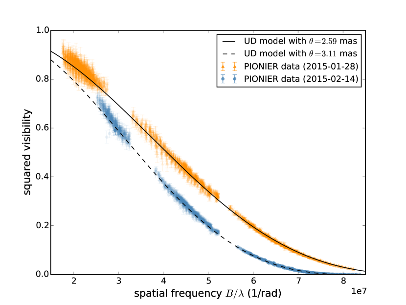
Figure 1: Squared visibilities measured with PIONIER at the minimum and maximum diameters for $\ell$ Car. The data are fitted with a uniform disk model leading to the diameters of $\theta_{\rm{min}}=2.59$ mas (MJD=57051, in orange) and $\theta_{\rm{min}}=3.11$ mas (MJD=57068, in blue).

Table 1: Journal of our new PIONIER observations

date	ATs config.	Disp.	Seeing
2014-04-02	A1-G1-K0-J3	LARGE	0.7-2.2
2014-04-04	A1-G1-K0-J3	SMALL	0.7-1.7
2014-05-07	A1-G1-K0-J3	SMALL	0.4-1.9
2014-07-28	A1-G1-K0-J3	SMALL	0.4-1.6
2014-07-30	A1-G1-K0-J3	SMALL	0.4-1.6
2014-08-01	A1-G1-K0-J3	SMALL	0.7-3.5
2014-08-04	A1-G1-K0-J3	SMALL	0.7-3.0
2014-08-19	A1-G1-K0-J3	SMALL	0.6-3.0
2014-08-24	A1-G1-K0-J3	SMALL	0.5-1.2
2015-01-13	A1-G1-K0-I1	GRISM	0.6-1.5
2015-01-14	A1-G1-K0-I1	GRISM	0.5-1.6
2015-01-15	A1-G1-K0-I1	GRISM	0.5-1.7
2015-01-16	A1-G1-K0-I1	GRISM	0.6-2.0
2015-01-26	A1-G1-K0-I1	GRISM	0.4-1.9
2015-01-27	A1-G1-K0-I1	GRISM	0.6-2.7
2015-01-28	A1-G1-K0-I1	GRISM	0.4-1.4
2015-01-29	A1-G1-K0-I1	GRISM	0.8-1.6
2015-01-30	A1-G1-K0-I1	GRISM	0.5-1.9
2015-02-04	D0-H0-G1-I1	GRISM	Unknown
2015-02-05	D0-H0-G1-I1	GRISM	Unknown
2015-02-12	A1-G1-K0-J3	GRISM	Unknown
2015-02-13	A1-K0-J3	GRISM	0.7-2.8
2015-02-14	A1-G1-K0-J3	GRISM	Unknown
2015-02-15	A1-G1-K0-J3	GRISM	0.5-1.8
2015-02-16	A1-G1-K0-J3	GRISM	Unknown
2015-02-17	A1-G1-K0-J3	GRISM	0.7-2.4
2015-02-18	A1-G1-K0-J3	GRISM	0.9-3.0
2015-02-20	A1-G1-K0-J3	GRISM	0.8-2.9

Table 2: PIONIER observations. We give here the mean MJD (defined as JD$-$2 400 000.5) of each observing night, the corresponding phase (taking $\phi_{0}$ at the maximum of luminosity in $V$), the range of baselines, the best uniform disk diameter adjusted on the squared visibility measurements, its uncertainty, and the reduced $\chi^{2}$ of the fit.

MJD	Baselines (m)	Phase	$\theta_{UD}\pm\sigma_{\rm{stat}}\pm\sigma_{\rm{syst}}$ (mas)	$\chi^{2}$
X Sgr
56867.1442	56.76 - 139.97	0.49	1.3428 $\pm$ 0.0025 $\pm$ 0.0595	2.85
56869.1692	56.76 - 139.97	0.78	1.2791 $\pm$ 0.0031 $\pm$ 0.0170	1.18
56871.1730	56.76 - 139.97	0.07	1.3185 $\pm$ 0.0034 $\pm$ 0.0170	1.07
56874.1975	56.76 - 139.97	0.50	1.3507 $\pm$ 0.0125 $\pm$ 0.0170	2.56
56894.1539	56.76 - 139.97	0.34	1.4098 $\pm$ 0.0033 $\pm$ 0.0170	1.11
W Sgr
56867.0798	56.76 - 139.97	0.53	1.1978 $\pm$ 0.0018 $\pm$ 0.0170	1.34
56869.0861	56.76 - 139.97	0.79	1.0778 $\pm$ 0.0036 $\pm$ 0.0170	2.80
56871.1161	56.76 - 139.97	0.06	1.0995 $\pm$ 0.0036 $\pm$ 0.0170	0.91
56874.1477	56.76 - 139.97	0.46	1.1606 $\pm$ 0.0044 $\pm$ 0.0170	2.45
56894.1044	56.76 - 139.97	0.09	1.1184 $\pm$ 0.0021 $\pm$ 0.0170	0.82
56889.1339	56.76 - 139.97	0.43	1.1711 $\pm$ 0.0047 $\pm$ 0.0170	1.02
$\zeta$ Gem
57038.2455	46.64 - 129.08	0.73	1.5372 $\pm$ 0.0025 $\pm$ 0.0425	1.97
57039.2786	46.64 - 129.08	0.83	1.5871 $\pm$ 0.0029 $\pm$ 0.0425	2.01
57071.1621	56.76 - 139.97	0.97	1.6047 $\pm$ 0.0020 $\pm$ 0.0690	1.17
57067.1395	56.76 - 139.97	0.57	1.5660 $\pm$ 0.0020 $\pm$ 0.0425	0.99
$\beta$ Dor
57036.0889	46.64 - 129.08	0.91	1.6857 $\pm$ 0.0016 $\pm$ 0.0120	2.41
57037.0627	46.64 - 129.08	0.01	1.7584 $\pm$ 0.0012 $\pm$ 0.0120	1.21
57038.0605	46.64 - 129.08	0.11	1.8160 $\pm$ 0.0010 $\pm$ 0.0120	2.98
57071.0192	56.76 - 139.97	0.46	1.7939 $\pm$ 0.0020 $\pm$ 0.0120	1.03
57074.0888	56.76 - 139.97	0.77	1.6022 $\pm$ 0.0040 $\pm$ 0.0120	1.78
57067.0280	56.76 - 139.97	0.05	1.7098 $\pm$ 0.0020 $\pm$ 0.0120	2.43
$\ell$ Car
56750.0604	56.76 - 139.97	0.41	3.1059 $\pm$ 0.0032 $\pm$ 0.0990	5.88
56752.1463	56.76 - 139.97	0.47	3.0803 $\pm$ 0.0028 $\pm$ 0.0575	6.76
56785.0895	56.76 - 139.97	0.40	3.1143 $\pm$ 0.0017 $\pm$ 0.0575	3.97
57049.2983	46.64 - 129.08	0.83	2.6383 $\pm$ 0.0003 $\pm$ 0.0160	0.03
57050.2604	46.64 - 129.08	0.85	2.6009 $\pm$ 0.0009 $\pm$ 0.0160	0.04
57051.3043	46.64 - 129.08	0.88	2.5999 $\pm$ 0.0004 $\pm$ 0.0160	0.03
57052.3017	46.64 - 129.08	0.91	2.6038 $\pm$ 0.0003 $\pm$ 0.0160	0.02
57053.3081	46.64 - 129.08	0.94	2.6156 $\pm$ 0.0004 $\pm$ 0.0160	0.02
57058.3484	41.03 - 82.48	0.08	2.8430 $\pm$ 0.0025 $\pm$ 0.0160	0.05
57059.3568	41.03 - 82.48	0.11	2.8913 $\pm$ 0.0035 $\pm$ 0.0160	0.05
57066.1018	56.76 - 139.97	0.30	3.0929 $\pm$ 0.0002 $\pm$ 0.0160	0.02
57068.2169	56.76 - 139.97	0.36	3.1117 $\pm$ 0.0003 $\pm$ 0.0160	0.03
57069.1280	56.76 - 139.97	0.39	3.1089 $\pm$ 0.0002 $\pm$ 0.0160	0.03
57070.1479	56.76 - 139.97	0.41	3.1104 $\pm$ 0.0003 $\pm$ 0.0160	0.03
57072.1099	56.76 - 139.97	0.47	3.0888 $\pm$ 0.0003 $\pm$ 0.0160	0.03

Table 3: Properties of the interferometric calibrators used during our PIONIER observations. We indicate the uniform disk diameter in the $H$ band and the corresponding uncertainty.

Star	$m_{v}$	$m_{H}$	$\theta_{UD}\pm\sigma$ (mas)	Ref.
HD35199	7.2	4.11	0.854 $\pm$ 0.012	(a)
HD39608	7.35	3.96	0.939 $\pm$ 0.012	(a)
HD50607	6.55	4.59	0.594 $\pm$ 0.042	(b)
HD50692	5.76	4.51	0.604 $\pm$ 0.043	(b)
HD54131	5.49	3.22	1.356 $\pm$ 0.096	(b)
HD81101	4.8	2.66	1.394 $\pm$ 0.099	(b)
HD81502	6.29	3.24	1.23 $\pm$ 0.016	(a)
HD89805	6.3	2.87	1.449 $\pm$ 0.019	(a)
HD156992	6.36	3.12	1.24 $\pm$ 0.017	(a)
HD166295	6.68	2.93	1.266 $\pm$ 0.017	(a)
HD166464	4.98	2.68	1.434 $\pm$ 0.102	(b)
HD170499	7.73	3.25	1.235 $\pm$ 0.017	(a)

2.2 Radial velocity measurements from the literature

The present study makes use of the following references providing RV data: Anderson (2014), Barnes et al. (2005), Bersier et al. (1994b), Bersier (2002), Evans et al. (1990), Gorynya et al. (1998), Kiss (1998), Nardetto et al. (2009), Petterson et al. (2005), and Storm et al. (2011).

The data coming from these different sources are consistent with each other, since almost all the RVs were determined with the same method (i.e., a cross-correlation of the spectra with a binary mask and a Gaussian fit of the resulting cross-correlation profile), and are given in the International Astronomical Union standard RV system. Only the velocities of Petterson et al. (2005) have been treated differently and result from a measurement of the line bisector. A change in the measurement method has an effect on the amplitude of the RV curve, especially if the spectral lines become highly asymmetric during the pulsation (Nardetto et al. 2006). Nevertheless, we needed these data to get a sufficiently complete coverage of the RV curve of $\beta$ Dor and W Sgr. Fortunately, none of these stars shows a significant amplitude modulation between these data and the other data sets (based on cross-correlation) that were used jointly. The CORAVEL data from Bersier et al. (1994b) and Bersier (2002) are given with an offset of +0.4 km s^-1 compared to IAU standard, while the zero point of Gorynya et al. (1998) data is given between +0.5 and +1.5 km s^-1 because different instruments were used in the observing campaign. Although we did not use it in the present study, we underline that all the CORAVEL zero points have been recently listed by Evans et al. (2015a). Except for $\zeta$ Gem, $\beta$ Dor, T Vul, and Y Sgr, we cannot see vertical shifts of the RV curves coming from different data sets. For the stars mentioned above, we simply corrected the different RV curves so that, for each author, the mean value of the model would coincide with $V_{\rm{mean}}=0$ km s^-1. This process allows us to ”clean” the curve for possible biases like zero point uncertainties or Keplerian motion due to a companion and to keep only the pulsation component. A discussion about the offsets between different RV data sets is presented in Kiss & Vinkó (2000). Kiss (1998) gives two different values for the RVs, resulting from the cross-correlation of two different parts of the spectra. We have opted to keep the mean value of both measurements. Finally, we consider a systematic error of $\pm 0.3$ km s^-1 that we quadratically add to the uncertainties of all the RV data to take all the systematic effects due to the combination of different data sets into account. The Cepheids of our sample have a reasonably good coverage in RV, which is essential for a proper estimation of the radius curve (Sect. 3).

2.3 Photometry from the literature

The present study makes use of an extensive collection of optical and near-infrared (hereafter IR) light curves. We use $BV$ photometric data from Kiss (1998), Barnes et al. (1997), Berdnikov (2008), Dean et al. (1977), Madore (1975), Moffett & Barnes (1984), Shobbrook (1992), Szabados (1977), Szabados (1981), and Szabados (1991). Most of these magnitudes are expressed in the standard Johnson-Morgan-Cousins system, therefore, we fit them with the Johnson and Cousins filters provided by the General Catalog of Photometric Data (GCPD) and revised by Mann & von Braun (2015). We also use data from the Hipparcos and Tycho catalogs (ESA 1997), which we fit with the dedicated Hipparcos and Tycho $B$ and $V$ band filters, also revised by Mann & von Braun (2015). Finally, we use Geneva magnitudes from Bersier et al. (1994a) and Bersier (2002) (only in the $V$ band), which were fitted with the suited Geneva $V$ band filter provided by the Spanish Virtual Observatory. We do not use the photometry in the $R$ and $I$ bands provided by some of these authors, since the detector’s quantum efficiency is generally uncertain in this wavelength range and the filter+detector effective bandpass is therefore poorly defined. As a consequence, these data tend to degrade the quality of the overall fit. In any event, the temperature and reddening information are mainly contained in the $B$ and $V$ bands, while the envelope is seen in IR. We also include photometry in the IR $JHK$ bands, which is less sensitive to the interstellar reddening and more sensitive to the effective temperature. We gathered data from Barnes et al. (1997), Monson & Pierce (2011), and Welch et al. (1984), which are all given in the CTIO photometric system; and from Lloyd Evans (1980), Feast et al. (2008), and Laney & Stobie (1992), which we converted from the SAAO to the CTIO systems through the laws given in Carter (1990).

Most authors give a standard deviation of 0.01 to 0.02 magnitudes for the individual measurements. The data from Hipparcos have very small error bars. To give them an equivalent weight in the fitting process, we multiplied all of the uncertainties by an arbitrary factor of $3$, which allows us to obtain a reduced $\chi^{2}$ close to 1 for the fit of this particular data set. To take the different instrumental calibrations into account, we added a systematic uncertainty of 0.02 magnitudes to all our photometric data. This value is consistent with the average offset generally observed when combining data from different instruments and magnitude systems (see, for instance, Barnes et al. 1997). The references of the data used for our nine Cepheids are summarized in Table 4. All Cepheids have an excellent phase coverage in all the selected optical and IR bands.

Table 4: Data used on each star to apply the SPIPS method. We gathered all the best quality radial velocities, photometry in bands $BVRI$ and $JHK$, and interferometric diameters (Diam.) from the literature.

Star	RVs	$BV$	$JHK$	Diam.
$\beta$ Dor	d, h, i	d, l, n, q, u	v, x	A, C, F
$\zeta$ Gem	c, f, g, h, j	l, g, p, q, s, u, m	w	B, C
X Sgr	j	d, l, p, q, u	w, z	A, C
Y Sgr	d, h, j	d, l, p, q, u	z	-
W Sgr	c, i	l, p, q, u, m	z	A, C
FF Aql	e, f, g	l, p, r, t, u	z	E
RT Aur	f, g	k, l, g, p, r, u	j, y	-
T Vul	b, c, g	k, l, g, p, r, u, m	j, z	E
$\ell$ Car	a, d, h, i	d, l, o, u, n	x	A, C, D

3 The SPIPS algorithm

To reproduce our complete observational data set, we use the Spectro-Photo-Interferometry of Pulsating Stars modeling tool (SPIPS; Merand et al. 2015), inspired from the classical PoP technique (commonly known as ”Baade-Wesselink”). The general idea of this method is to compare the linear and angular variations of the Cepheid diameters to retrieve the distance. The SPIPS code can take all the different types of data and observables that can be found in the literature into account, in particular, magnitudes and colors in all optical and IR bands and filters, RVs, and interferometric ADs. The resulting redundancy in the observables ensures a higher level of robustness. For instance, the AD is constrained by both the interferometry and photometry (via the use of atmospheric models). The SPIPS code also allows us to fit an excess in $K$ and $H$ band, to bring out the possible presence of a CSE. It also outputs the color excess $E(B-V)$, derived through the reddening law from Fitzpatrick (1999), considering the classical Galactic value of the total-to-selective absorption $R_{\rm{V}}=3.1$.

It is necessary to set the value of the $p$-factor (also abbreviated as $p$ in the following) used to convert the spectral RVs into photospheric pulsation velocities through $V_{\rm{puls}}=p\,V_{\rm{rad}}$. The $p$-factor is fully degenerate with the distance in the PoP technique (including SPIPS). In fact, $p$ and $d$ are symmetrical in the fitting process, and only the ratio $p/d$ can be derived unambiguously unless one of these two parameters can be determined independently and input in SPIPS as a fixed parameter. The $p$-factor is also sensitive to the spectral lines that are considered, since they are all formed in different layers of the atmosphere and do not pulsate at the exact same velocity. Observing in different lines (e.g., different line-forming regions) consequently leads to different $p$-factors. In the present study, we mainly use cross-correlation velocities that allow us to average out the differential atmospheric effects. The method used to derive the RVs is an important point in the PoP method, as the curves obtained with different techniques can have more than 5% difference in amplitude (Nardetto et al. 2007). It is important to stress that the results from the present study are suited for the cross-correlation method and a Gaussian fit of the cross-correlation profile.

We selected nine Cepheids whose parallax has been measured by Benedict et al. (2007) with the Fine Guidance Sensor (FGS) on board the Hubble Space Telescope: RT Aur, T Vul, FF Aql, Y Sgr, X Sgr, W Sgr, $β$ Dor, $ζ$ Gem, and $ℓ$ Car. Knowing the distance, we can break the degeneracy of the PoP method and deduce the value of their $p$-factor, as already carried out on the prototype classical Cepheid $\delta$ Cep by Mérand et al. (2005b) and on the type II Cepheid $\kappa$ Pav by Breitfelder et al. (2015). These studies give values of $1.27\pm 0.06$ and $1.26\pm 0.07$, respectively, for the $p$-factor. For each Cepheid, we fit the RV curves using spline functions defined by semifixed nodes. Although this method is numerically less stable than Fourier series, it leads to smoother models and avoids the introduction of unphysical oscillations when the data are too dispersed or not dense enough. The photometry curves are fitted with Fourier series. This does not introduce spurious oscillations thanks to the large quantity and good phase coverage of photometric data collected for each star. To take into account each main observable (RV, interferometry, IR photometry, and optical photometry) in a balanced way, we allocate to these different data sets the same weight in the fitting process. We do this by multiplying the error bars by a factor inversely proportional to the number of data points contained in that observable group. For each Cepheid, we set a reference MJD taken as close as possible to the center of the time interval covered by the data and corresponding to a maximum of luminosity. We fit both the period and a linear variation $dP/dt$ with the SPIPS code; the best parameters are those allowing the smallest dispersion of the data. This approach is different from the usual study of the O-C diagram and does not always lead to identical results (Sect. 4). The final ephemerides used to phase the data are given in Table 5. We indicate the reference date, the period and its variation, and the corresponding crossing of the Cepheid in the instability strip (deduced from the predictions of Fadeyev 2014). The table also gives the epoch range covered by the data, which is relevant information for the calculation of the $dP/dt$ variation. The results are described star-by-star in Sect. 4 and the graphics resulting from the SPIPS modeling are shown in the annexes. The values of all the best-fit parameters are given in Table 7, where we indicate both the statistical and systematic errors. In the case of the $p$-factor, the systematic error is due to the parallax. For the temperature and reddening, the systematic error has been set by running a ”jackknife” algorithm on the photometric data of $\delta$ Cep, a star that has been extensively studied in Mérand et al. (2005b) and Merand et al. (2015). This method leads to uncertainties of 0.016 for reddenings and 50 K for temperatures. When no interferometric diameters were available, we considered a systematic error of 2% on the diameters (Kervella et al. 2004a).

Table 5: Ephemeris used to phase the data of each Cepheid. We also give the epoch range covered by the data for each Cepheid.

Star	$\rm{MJD}_{\rm{0}}$	Period (days)	dP/dt (sec/yr)	Crossing	Epoch range
		(days)	(sec/yr)		(yrs)
RT Aur	48027.678	3.728305 $\pm$ 0.000005	0.124 $\pm$ 0.036	3	36
T Vul	49134.074	4.435424 $\pm$ 0.000005	0.060 $\pm$ 0.035	3	25
FF Aql	45912.675	4.470848 $\pm$ 0.000010	$-$0.140 $\pm$ 0.036	2	66
Y Sgr	47303.129	5.773383 $\pm$ 0.000009	0.016 $\pm$ 0.048	3	30
X Sgr	49310.835	7.012770 $\pm$ 0.000012	0.371 $\pm$ 0.098	3	37
W Sgr	48257.806	7.594984 $\pm$ 0.000009	0.331 $\pm$ 0.111	3	37
$\beta$ Dor	49133.243	9.842675 $\pm$ 0.000019	$-$0.084 $\pm$ 0.149	2	42
$\zeta$ Gem	49134.561	10.149806 $\pm$ 0.000017	$-$1.238 $\pm$ 0.144	2	43
$\ell$ Car	47774.310	35.551609 $\pm$ 0.000265	27.283 $\pm$ 0.984	3	42

4 Results

4.1 RT Aur

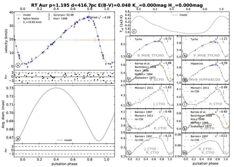
Figure 6: SPIPS model of RT Aur.

RT Aur is a very short period Cepheid (3.7 days). Its cycle-to-cycle photometric variations were recently studied by Evans et al. (2015b), who found a high repeatability in amplitude, but a slow drift of 0.000986 days per century (0.852 s/yr) in pulsation period. Turner et al. (2007) propose a much lower value of $0.082\pm 0.012$ s/yr, which is closer to our own value of $0.124\pm 0.036$ s/yr. This period change is that expected for a Cepheid crossing the instability strip for the third time (Fadeyev 2014). Turner et al. (2007) observed a sinusoidal trend in the O-C diagram, which is interpreted as a light-time effect produced by a long period orbit companion. Evans et al. (2015b) also reported a slight decrease in $v_{\gamma}$, but they did not reach a conclusion about the presence of a companion. Gallenne et al. (2015) detected the companion from CHARA/MIRC interferometric observations via the CANDID code. The data revealed a very close companion lying only 2.1 mas away from the Cepheid. This finding is, however, unconfirmed and demands further studies. Gallenne et al. (2015) published a UD diameter of $0.699\pm 0.011$ at $\phi=0.32$, which is consistent with the value found in the present study at the same phase. Kovtyukh et al. (2008) and Benedict et al. (2007) gave respective color excesses of $E(B-V)=0.050\pm 0.036$ and $0.051$, which are both consistent with the color excess resulting from our SPIPS fit ($E(B-V)=0.048\pm 0.016$). We find a $p$-factor of $1.20\pm 0.08_{\rm{stat}}\pm 0.09_{\rm{sys}}$, which is in agreement at a 2$\sigma$ level with most values deduced from published period-$p$ relations. The value found in the present study and the value from Nardetto et al. (2009) agree within their error bars. The final SPIPS adjustment is shown in Fig. 6.

4.2 T Vul

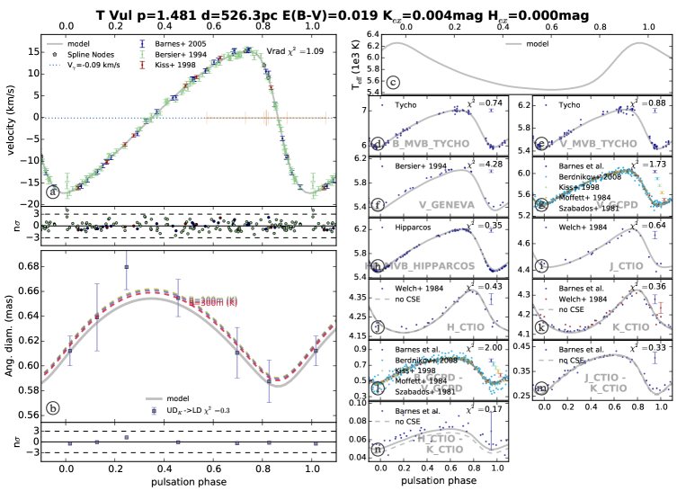
Figure 7: SPIPS model of T Vul.

T Vul is a bright, short-period (4.4 days) northern Cepheid. For this star, we corrected the different RV data sets from their mean value (calculated using the same model for each author): $-0.988\pm 0.032$ km s^-1 for Barnes et al. (2005), $-2.664\pm 0.033$ km s^-1 for Bersier et al. (1994b), and $-0.759\pm 0.030$ km s^-1 for Kiss (1998). A simple linear period variation did not allow us to phase the CHARA/FLUOR interferometric diameters properly from Gallenne et al. (2012) with the rest of the data. We therefore kept the pulsation phases given by the authors and added an offset of $\phi=-0.2328$ to reach the best phase agreement. The interferometric data in Gallenne et al. (2012) lead to a mean diameter of $0.629\pm 0.013$ mas for T Vul, consistent with our SPIPS diameter of $0.607\pm 0.012$ mas. Like us, Gallenne et al. (2012) use the parallax from Benedict et al. (2007) ($\pi=1.90\pm 0.23$, $d=526.31\pm 63.71$ pc), and deduce a linear radius $R=35.6\pm 4.4\leavevmode\nobreak\ R_{\odot}$, coherent with our own value of $35.39\pm 0.07_{\rm{stat}}\pm 4.98_{\rm{sys}}\leavevmode\nobreak\ R_{\odot}$. A faint spectroscopic companion of type A0.8 V has been discovered in the International Ultraviolet Explorer (IUE) observations from Evans (1992b), and Gallenne et al. (2015) did not detect any companion with a spectral type earlier than B9V within 50 mas. Kovtyukh et al. (2008), Benedict et al. (2007) and Evans (1992b) published similar values of $0.068\pm 0.015$, $0.064$ and $0.060$, respectively, for the color excess. Our study leads to a lower value of $0.019\pm 0.016$. Various authors agree that the pulsation period of T Vul is subject to a slight decrease with time. Meyer (2006) mentioned that the change rate is in the interval of $-0.25\pm 0.13$ s/yr with a probability of 99%, while Turner (1998) suggests a similar value of $-0.24$ s/yr. We find a disagreeing value of $0.060\pm 0.035$ s/yr, which would place in T Vul rather in the third crossing of the instability strip (Fadeyev 2014). Whether or not we include the interferometric data in the SPIPS fit leads to consistent results, although the amplitude of the diameter variation tends to be slightly underestimated. We find a $p$-factor of $1.48\pm 0.04_{\rm{stat}}\pm 0.18_{\rm{sys}}$, which is compatible at a level of 1$\sigma$ with most values deduced from published period-$p$ relations. In addition, our result agrees at 1.2$\sigma$ with the value of $1.19\pm 0.16$ found in Benedict et al. (2007). The final adjustment is shown in Fig. 7.

4.3 FF Aql

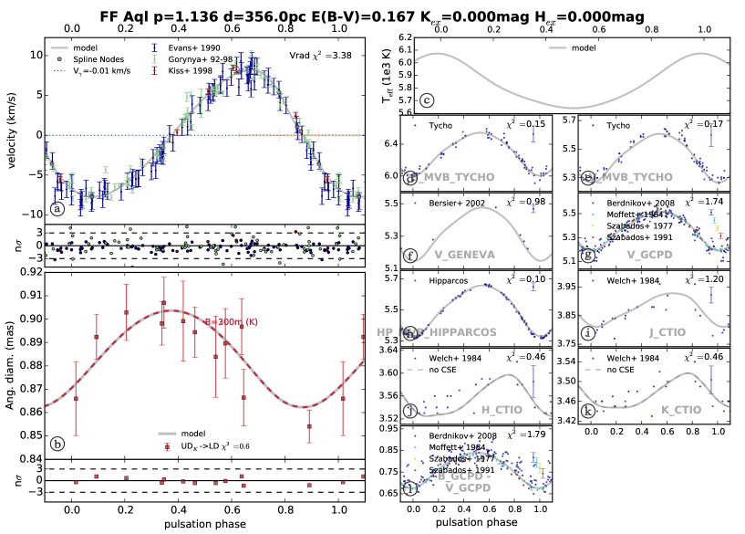
Figure 8: SPIPS model of FF Aql.

FF Aql is known to be part of a possible quadruple system. The spectroscopic companion was recently studied with the VLT/NACO instrument, by Gallenne et al. (2014). No direct detection could be made, but the authors exclude spectral types outside from the A9V-F3V range. The signature of orbital motion is clearly apparent in the RV curve, and was extensively studied by Evans et al. (1990). We corrected all the data used in the present study (Evans et al. 1990), Gorynya et al. 1998 Kiss 1998) with a modified version of the Wright & Howard formalism (Wright & Howard 2009), in which we included the pulsation of the star (see Gallenne et al. 2013b). We solved for the spectroscopic orbital elements and pulsation parameters with uncertainties derived via the bootstrapping technique (with replacement and 10000 bootstrap samples). Our derived parameters are an orbital period $P=1438.76\pm 1.60$ days, a JD of periastron passage $T=2445204.81\pm 87.17$ days, an eccentricity $e=0.113\pm 0.042$, an argument of periapsis $\omega=262.7\pm 23.6$, a velocity semi-amplitude $K=4.949\pm 0.156$ km s^-1, and a systemic velocity $V_{\gamma}=-15.6\pm 0.1$ km s^-1. The reduced $\chi^{2}$ is 12.38 because of the relatively high intrinsic dispersion of the data. Both disentangled velocity curves are shown in Fig. 8. Gallenne et al. (2012) published an average LD diameter of $0.878\pm 0.013$ mas, consistent with our diameter of $0.870\pm 0.013$ mas. Using the parallax from Benedict et al. (2007) ($\pi=2.81\pm 0.18$, $d=356\pm 23$ pc), we obtain a linear radius of $33.84\pm 2.67\leavevmode\nobreak\ R_{\odot}$. Kovtyukh et al. (2008) and Benedict et al. (2007) published the same value for the color excess: $E(B-V)=0.224$, and Turner et al. (2013) give a similar value of $0.25\pm 0.01$. We find a slightly lower reddening of $0.167\pm 0.017$. Turner et al. (2013) also give an average temperature $\langle T_{\rm{eff}}\rangle=6195\pm 24$ K. Our temperature model is quite colder, but in agreement with the temperature published by Gallenne et al. (2011) ($\langle T_{\rm{eff}}\rangle=5890\pm 235$ K). Turner et al. (2013) place the Cepheid on the blue side of the instability strip and argue that the rate of period change ($+0.0703\pm 0.0160$ s/yr) is consistent with this result. Berdnikov et al. (2014) also find a value of $dP/dt=0.072\pm 0.011$ s/yr. We find that the Cepheid is close to the center of the instability strip with a very different rate of period change ($-0.140\pm 0.036$ s/yr), which places the Cepheid in the second crossing of the instability strip (Fadeyev 2014). We do not find any IR excess. A CSE has been brought out by Gallenne et al. (2011), but it only becomes significant for $\lambda>10\leavevmode\nobreak\ \mu m$.

The SPIPS code for this particular Cepheid shows an irregular behavior. If we exclude the interferometric data, the amplitude of the diameter variation is highly underestimated and results in a much lower (and even unphysical) value of the $p$-factor: $p=0.6\pm 0.02_{\rm{stat}}\pm 0.07_{\rm{sys}}$. Including the interferometry in the fit leads to $p=1.14\pm 0.07_{\rm{stat}}\pm 0.07_{\rm{sys}}$, which is rather low (but still in a 3$\sigma$ agreement with most values deduced from the literature owing to the relatively large uncertainty). This could be due to a misestimation of the distance, which is actually subject to controversy. In particular, there is a tension between Hipparcos and HST parallaxes (yielding to $d=474\pm 74$ pc and $d=356\pm 23$ pc, respectively). Ngeow et al. (2012) also removed FF Aql from their study of the $p$-factor because of this discrepancy, whose origin may be linked to the binary nature of the star. The relatively large uncertainties on the data could also explain a lower overall quality of the fitting process. The final $p$-factor value should therefore be considered with caution. The adjustment for FF Aql is shown in Fig. 8.

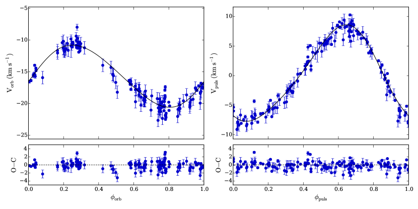
Figure 2: Left: Orbital velocity of FF Aql as a function of the orbital phase, corrected for the pulsation. Right: Pulsational radial velocity curve as a function of the pulsation phase.

4.4 Y Sgr

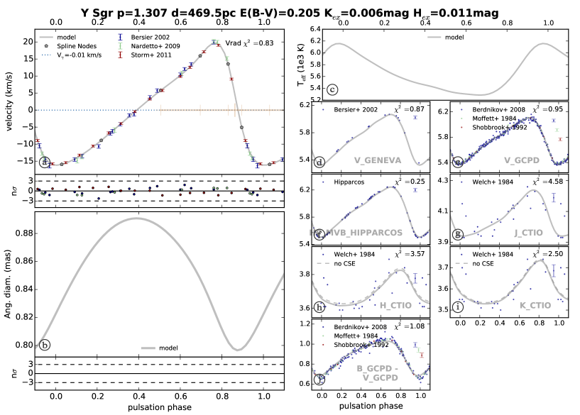
Figure 9: SPIPS model of Y Sgr.

The 5.7-day period Cepheid Y Sgr has not been as extensively studied as the rest of our sample. For this star, no interferometric observations are available, but the SPIPS code nevertheless converged properly. We corrected the different RV data sets to obtain average values and found the following offsets: $-3.59\pm 0.04$ km s^-1 for Bersier (2002), $-1.79\pm 0.02$ km s^-1 for Nardetto et al. (2009), and $-2.55\pm 0.03$ km s^-1 for Storm et al. (2011). Szabados (1989) underlines that the change in the $\gamma$-velocity could be due to the presence of a very long period ($>$10000 days) companion (he reports orbital variations in the O-C diagram). Evans (1992a) did not detect the companion in the data from the International Ultraviolet Explorer, but she set an upper limit on the spectral type, which could not be earlier than A2. Bersier (2002) supports the presence of a companion with an orbital period around 10000 days as well. There is no period change reported for this Cepheid. Our study nevertheless leads to the value of $dP/dt=0.016\pm 0.048$ s/yr, which places Y Sgr in the third crossing of the instability strip (Fadeyev 2014). Kovtyukh et al. (2008) publish a color excess $E(B-V)=0.182\pm 0.021$, and Benedict et al. (2007) give the value of 0.205. Our own computation leads to $E(B-V)=0.205\pm 0.017$, which is in agreement with what we found in the literature. We find a linear radius of $43.10\pm 6.73\leavevmode\nobreak\ R_{\odot}$, in agreement with the period-radius relationship from Molinaro et al. (2012). Our effective temperature model is in average 400 K colder than the temperatures given by Andrievsky et al. (2005). Our study leads to a $p$-factor of $p=1.31\pm 0.06_{\rm{stat}}\pm 0.18_{\rm{sys}}$, which is remarkably close to the values from Groenewegen (2013), Nardetto et al. (2007), and Ngeow et al. (2012), and is compatible at a 1$\sigma$ level with most values deduced from the literature. The final adjustment for Y Sgr is shown in Fig. 9.

4.5 X Sgr

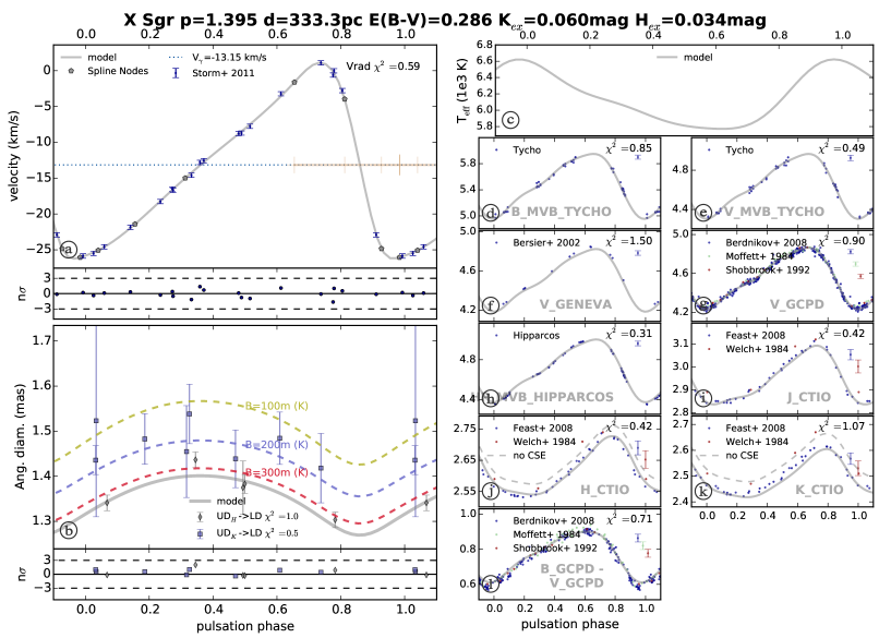
Figure 10: SPIPS model of X Sgr.

X Sgr is a 7-day period Cepheid known for the atypical features observed in its spectra, which are probably the consequence of the propagation of a double shockwave in the atmosphere of the star (Mathias et al. 2006). Although this effect is expected to have an impact on the RV measurements, it does not seem to affect our results much, since our output parameters are consistent with the average values found for the rest of the sample. We determine a reddening $E(B-V)=0.286\pm 0.016$, which is slightly higher than the values of $0.219$ found in Kovtyukh et al. (2008), and $0.197$ found in Benedict et al. (2007). Li Causi et al. (2013) determine a LD diameter of $1.48\pm 0.08$ mas and a radius of $53\pm 3\leavevmode\nobreak\ R_{\odot}$, considering the same distance as us (from Benedict et al. 2007; $\pi=3.00\pm 0.18$, yielding to $d=333\pm 20$ pc). These results are in slight tension (but consistent) with ours, as we determine an average diameter of $1.315\pm 0.025$ mas, leading to a slightly lower radius of $48.37\pm 3.84\leavevmode\nobreak\ R_{\odot}$. Kovtyukh et al. (2008) find a stellar diameter of $\theta_{\rm{LD}}=1.24\pm 0.14$ mas, and Kervella et al. (2004b) deduce from their VLTI/VINCI data a diameter $\theta_{\rm{UD}}=1.471\pm 0.033$ mas. Our SPIPS analysis reveals significant excesses of 0.060 and 0.034 magnitude in $K$ and $H$ bands, respectively. A CSE around this Cepheid has been detected as a result of VLTI/MIDI observations by Gallenne et al. (2013a), who found an excess of 7% at $10.5\leavevmode\nobreak\ \mu m$. The same authors lead a detailed study of the envelope owing to the radiative transfer simulation code DUSTY. They find an average effective temperature for the star of $T_{\rm{eff}}=5900$ K, which is slightly lower than our value of $T_{\rm{eff}}=6117\pm 52$. These authors also find a lower reddening of $0.200\pm 0.032$, which is actually closer to the value of Kovtyukh et al. (2008). The exclusion of the interferometry in the global fit leads to similar results, however, a slightly lower (although consistent) $p$-factor. This small instability could be due to the lack of RVs measurements, in particular, at the extrema. We find a linear period variation of $0.371\pm 0.098$ s/yr, corresponding for X Sgr to the third crossing of the instability strip (Fadeyev 2014). Szabados (1989) finds a higher value of $0.74\pm 0.09$ s/yr, which nevertheless corresponds to the same evolutionary status. Our study leads to a $p$-factor of $p=1.39\pm 0.04_{\rm{stat}}\pm 0.08_{\rm{sys}}$, which is remarkably similar to the value published by Storm et al. (2011), and agrees with most values deduced from the literature at a level of 1$\sigma$. The SPIPS adjustment for this Cepheid is shown in Fig. 10.

4.6 W Sgr

W Sgr is a 7.5-day Cepheid, which is known to belong to a triple system composed of a spectroscopic binary and a visual hot companion. The RVs from Bersier et al. (1994b) are corrected for the orbital motion and perfectly match the data from Petterson et al. (2005). The orbital elements were deduced again from HST observations of Benedict et al. (2007), who found a period of 1582 days. From Evans et al. (2009), this close companion (only 5 AU from the Cepheid) could not be earlier than an F0V star. The hot component located at 0.16 as could not be detected in NACO observations (Gallenne et al. 2014). The study of the O-C diagram from Szabados (1989) does not reveal a period variation. Turner (1998) publishes a very low value of $-1.5$ s/yr, which corresponds to the second crossing of the instability strip. We find a very different value of $0.331\pm 0.111$ s/yr, which places the Cepheid in the third crossing of the instability strip (Fadeyev 2014).

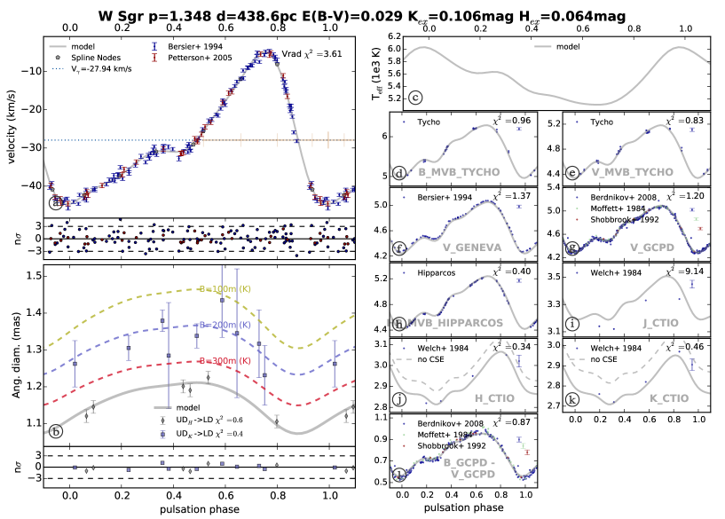
Figure 11: SPIPS model of W Sgr.

The VLTI/VINCI observations from Kervella et al. (2004b) lead to an average $\theta_{UD}=1.312\pm 0.029$ mas. We find a significantly lower diameter of $1.110\pm 0.017$ mas, in agreement with Gallenne et al. (2011). Our PIONIER observations are undertaken in $H$ band, while the VINCI observations were made in the $K$ band. The star shows a large IR excess of about 0.106 magnitudes in $K$ and 0.064 magnitude in $H$. Its larger apparent size in the $K$ band is likely caused by the contribution of its extended CSE in this band. The code SPIPS takes the IR excess into account to fit all the interferometric data together. The CSE was also brought out by Gallenne et al. (2011), who detected a spatially resolved emission around W Sgr in VLT/VISIR images. Kovtyukh et al. (2008) and Benedict et al. (2007) give reddenings of $E(B-V)=0.079\pm 0.017$ and $0.111$, respectively. Our value stands in the middle, at $0.029\pm 0.017$. Our study leads to a $p$-factor of $p=1.35\pm 0.06_{\rm{stat}}\pm 0.12_{\rm{sys}}$. This result is in agreement with most values deduced from the literature at a 1$\sigma$ level. In particular, it is remarkably close to the value found by Neilson et al. (2012). The final adjustment for W Sgr is shown in Fig. 11.

4.7 $\beta$ Dor

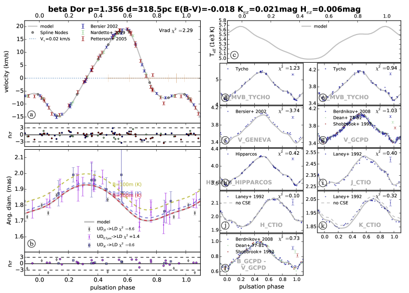
Figure 12: SPIPS model of $\beta$ Dor.

$\beta$ Dor is one of the brightest and biggest southern Cepheids, and it has therefore been extensively observed. Unlike most Cepheids, it has no visual or spectroscopic companion known, and we did not find any companion in our interferometric data. In order to reduce the dispersion of the RV curve of $\beta$ Dor, we corrected the three different RV data sets from their mean velocity (calculated from the model) to equal 0 km s^-1. We found the following offsets: $8.63\pm 0.03$ km s^-1 for Bersier (2002), $9.58\pm 0.12$ km s^-1 for Petterson et al. (2005), and $8.76\pm 0.04$ km s^-1 for Nardetto et al. (2009). We also decided to exclude the PIONIER measurement at $\phi=0.78$, whose quality was low because of bad weather conditions during the observations. Removing this point allows a higher stability of the fit. We observe that whether or not we use the interferometric data leads to the same final results, which confirms the robustness of the fitting process. The SPIPS best-fit parameters for $\beta$ Dor give a reddening $E(B-V)=-0.018\pm 0.016$, consistent with the value of 0.00 published by Kovtyukh et al. (2008). The negative value could suggest the presence of an undetected hot companion. Our linear diameter is smaller than that published by Taylor & Booth (1998) ($R=67.8\pm 0.7\leavevmode\nobreak\ R_{\odot}$). However, they suggest a higher distance ($349\pm 4$ pc) than the distance we use (from Benedict et al. 2007; $\pi=3.14\pm 0.16$, or $d=318\pm 16$ pc), which makes both results consistent in terms of AD. Kervella et al. (2004b) found a value of $\theta_{UD}=1.891\pm 0.024$ mas, which is larger than our diameter of $1.776\pm 0.012$ mas. The O-C diagram from Szabados (1989) does not suggest any period change. A more recent study led by the Secret Lives of Cepheids program (Engle 2015) finds a period change of $0.468\pm 0.016$ s/yr. In the present study, we find a value of $-0.084\pm 0.149$ s/yr, suggesting that $\beta$ Dor is in the second crossing of the instability strip (Fadeyev 2014). Turner (1998) finds a much lower value of $-3.4$ s/yr. We find an average effective temperature of $5318\pm 51$ K, slightly lower than the value of $5490$ found in Kervella et al. (2004b). Our study leads to a $p$-factor of $p=1.36\pm 0.04_{\rm{stat}}\pm 0.07_{\rm{sys}}$. This result is remarkably close to the values deduced from the period-$p$ relations published by Neilson et al. (2012) and Storm et al. (2011), and agrees with most other published values at a level of 1$\sigma$. The final adjustment for $\beta$ Dor is shown in Fig. 12 of Appendix A.

4.8 $\zeta$ Gem

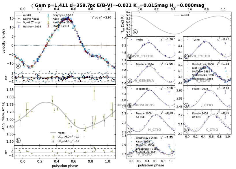
Figure 13: SPIPS model of $\zeta$ Gem.

As $\zeta$ Gem is the Northern Cepheid with the largest AD, it has been the subject of a lot studies. This bright winter star is known to have a visual companion at 87 arcseconds (Proust et al. 1981), although it is uncertain if the stars are gravitationally bound. We did not identify any close companion in our PIONIER data. However, we observe a slight variation of $V_{\rm{mean}}$ between the different data sets of RV that we used, which could be an actual variation of $V_{\gamma}$ due to orbital motion. We determined and subtracted the following offsets: Bersier et al. (1994b), $5.939\pm 0.085$ km s^-1; Gorynya et al. (1998), $5.512\pm 0.031$ km s^-1; Kiss (1998), $6.603\pm 0.136$ km s^-1; Nardetto et al. (2009), $6.477\pm 0.046$ km s^-1; and Storm et al. (2011), $7.363\pm 0.017$ km s^-1. However, such a small amplitude of variation (about 2 km s^-1) does not allow us to reach a conclusion about binarity, since it could also be due to instrumental systematics. We find a negative but close to zero reddening, consistent with the values from Kovtyukh et al. (2008) ($E(B-V)=0.031\pm 0.041$), Benedict et al. (2007) ($0.017$), and Majaess et al. (2012) ($0.019\pm 0.017$). Majaess et al. (2012) established the membership of $\zeta$ Gem to a host cluster lying at a distance $d=355\pm 15$ pc, which is consistent with the distance used in the present study (from Benedict et al. 2007; $\pi=2.78\pm 0.18$, $d=360\pm 23$ pc). We find a linear period variation of $-1.238\pm 0.144$ s/yr, placing $\zeta$ Gem in the second crossing of the instability strip (Fadeyev 2014). Engle (2015) propose a value of $-3.100\pm 0.011$ s/yr, suggesting that the Cepheid could be either in its second or fourth crossing. Our whole temperature model is shifted by about 150 K compared to the $T_{\rm{eff}}$ measurements found in Luck et al. (2008). From their VLTI/VINCI interferometric measurements, Kervella et al. (2004b) found an average diameter $\theta_{UD}=1.747\pm 0.061$ mas. This value is in agreement with the result of the present study ($1.663\pm 0.049$ mas). Our study leads to a $p$-factor of $p=1.41\pm 0.04_{\rm{stat}}\pm 0.09_{\rm{sys}}$, which is in agreement at 1$\sigma$ with the values published by Storm et al. (2011), Nardetto et al. (2007), and Neilson et al. (2012), but is also compatible with most other published values at a 2$\sigma$ level. The final adjustment is shown in Fig. 13.

4.9 $\ell$ Car

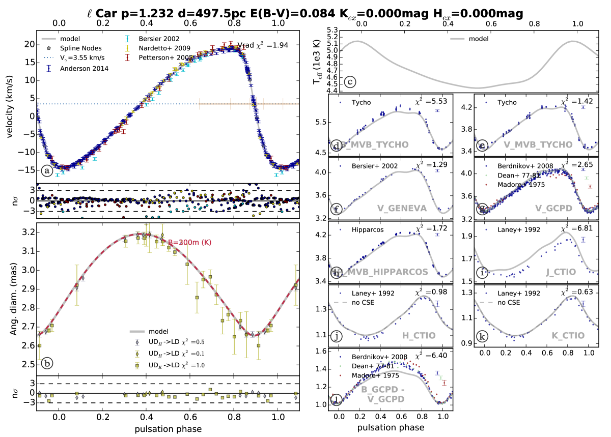
Figure 3: Result of the SPIPS model fit to the observations of $\ell$ Car

As discussed by Anderson (2014), the RV variations of $\ell$ Car are not perfectly reproduced cycle-to-cycle. This is potentially a difficulty for the application of the BW technique, which relies on observational data sets that are generally obtained at different epochs and therefore different pulsation cycles. This potentially induces an uncertainty on the amplitude of the linear radius variation and therefore on the derived parameters (distance or $p$-factor). However, as shown in Fig. 3, the residual of the adjustment of the SPIPS model is satisfactory in terms of RVs. The quality of the fit is generally also good for the different photometric bands and colors for $\ell$ Car. There is, however, a noticeable difference in the model predictions with the photometry for $\ell$ Car in the deflation phase up to the minimum diameter rebound. This is an interesting feature, which is probably caused by a deviation of the surface brightness of $\ell$ Car from the model atmosphere used in the SPIPS code. The interferometric ADs of $\ell$ Car are accurately reproduced by the model, but a systematic shift of 3.5% is present between the VINCI ($K$ band) and SUSI ($700$ nm) measurements. The two PIONIER measurements ($H$ band) obtained shortly after the maximum radius phase are between the VINCI and SUSI. This may be interpreted as a bias due to the chosen LD model (Neilson & Lester 2013). However, the irregularity of the RV curve reported recently by Anderson (2014) appears to be another possible reason for this effect, as the VINCI (epoch 2003) and SUSI (epoch 2004-2007) data were obtained during different pulsation cycles. The O-C diagram of $\ell$ Car is presented in Fig. 4. The parabola fits the O-C residuals very well, and the minor fluctuations reflect the uncertainties in determining the moment of brightness maxima from sparsely covered light curves and the contribution of the intrinsic period noise present in Cepheids. The secular increase in the pulsation period derived from the O-C diagram is $0.06225\pm 0.00214$ day/century, equivalent to $53.78\pm 1.85$ s/yr. The resulting ephemeris for brightness maxima of $\ell$ Car is, therefore, (expressed in Julian date)

$$\begin{split}C=&\ \ 2450405.8306\pm 0.0344\\ &+\Bigl{(}35.556234\pm.000373\Bigr{)}\times E\\ &+\Bigl{(}3.030\times 10^{-5}\pm.104\times 10^{-5}\Bigr{)}\times E^{2}.\end{split}$$

The SPIPS code leads to a lower value than the O-C diagram, $27.283\pm 0.984$ s/yr, which is also much lower than the value proposed by Turner (1998) (118.5 s/yr).

Figure 4: O-C diagram of $\ell$ Car.

The possible presence of an excess emission in the IR $H$ and $K$ bands is considered in the SPIPS code, but no significant excess is detected in the present study. This is in contradiction with the detection reported in the $K$ band by Kervella et al. (2006) for $\ell$ Car. However, Kervella et al. (2009) did not confirm the presence of a photometric excess in the $K$ band, although a considerable excess flux is found in the thermal IR ($10\,\mu$m) and longward. The detection in the $K$ band reported by Kervella et al. (2006) is based on the difference in visibility between observations of $\ell$ Car that were obtained at short and long baselines. The detection of this excess relies implicitly on the assumption that the radial pulsation of the star repeats itself with an accuracy on the order of 1%, i.e., that the stellar radius at a given phase is constant for different cycles. If this is not the case, as argued by Anderson (2014), then the random difference in angular size can mimic the presence (or absence) of an envelope if the observations with the short and long baselines are not obtained within the same cycle, which was the case for the observations of Kervella et al. (2006). For this same reason, based on our SPIPS model, we do not exclude the presence of a CSE at a level of a few percent in the $K$ band. Our study leads to a $p$-factor of $p=1.23\pm 0.01_{\rm{stat}}\pm 0.12_{\rm{sys}}$, which is in agreement with most results deduced from published period-$p$ relations.

5 Discussion

The $p$-factors resulting from the present study, and the main values deduced from published period-$p$ relations, are summarized in Table 6.

Table 6: $p$-factors calculated with SPIPS and main values deduced from published period-$p$ relations.

Star	present work	$(1)$	$(2)$	$(3)$	$(4)$	$(5)$	$(6)$
RT Aur	1.20 $\pm$ 0.12	1.363 $\pm$ 0.029	1.444 $\pm$ 0.074	1.339 $\pm$ 0.034	1.264 $\pm$ 0.089	1.356 $\pm$ 0.064	1.377 $\pm$ 0.003
T Vul	1.48 $\pm$ 0.18	1.345 $\pm$ 0.032	1.43 $\pm$ 0.079	1.335 $\pm$ 0.036	1.258 $\pm$ 0.092	1.344 $\pm$ 0.064	1.374 $\pm$ 0.003
FF Aql	1.14 $\pm$ 0.10	1.344 $\pm$ 0.033	1.429 $\pm$ 0.079	1.334 $\pm$ 0.036	1.258 $\pm$ 0.093	1.344 $\pm$ 0.064	1.373 $\pm$ 0.003
Y Sgr	1.31 $\pm$ 0.19	1.317 $\pm$ 0.038	1.408 $\pm$ 0.086	1.327 $\pm$ 0.038	1.249 $\pm$ 0.098	1.326 $\pm$ 0.064	1.368 $\pm$ 0.003
X Sgr	1.39 $\pm$ 0.09	1.297 $\pm$ 0.042	1.393 $\pm$ 0.091	1.322 $\pm$ 0.04	1.242 $\pm$ 0.102	1.313 $\pm$ 0.064	1.365 $\pm$ 0.003
W Sgr	1.35 $\pm$ 0.13	1.289 $\pm$ 0.044	1.386 $\pm$ 0.093	1.320 $\pm$ 0.041	1.240 $\pm$ 0.104	1.307 $\pm$ 0.064	1.363 $\pm$ 0.003
$\beta$ Dor	1.36 $\pm$ 0.08	1.262 $\pm$ 0.050	1.365 $\pm$ 0.100	1.312 $\pm$ 0.043	1.231 $\pm$ 0.110	1.289 $\pm$ 0.064	1.358 $\pm$ 0.003
$\zeta$ Gem	1.41 $\pm$ 0.10	1.258 $\pm$ 0.050	1.363 $\pm$ 0.100	1.312 $\pm$ 0.043	1.229 $\pm$ 0.110	1.287 $\pm$ 0.064	1.358 $\pm$ 0.003
$\ell$ Car	1.23 $\pm$ 0.12	1.128 $\pm$ 0.078	1.262 $\pm$ 0.133	1.277 $\pm$ 0.054	1.186 $\pm$ 0.138	1.200 $\pm$ 0.064	1.334 $\pm$ 0.003

For almost all the Cepheids in the present study, the SPIPS code converges toward the same $p$-factors whether or not we include the interferometric data. This agreement is a confirmation that the surface brightness-color relations, which are implicitly included in the SPIPS atmosphere models, are reliable tools to determine ADs with photometry. This is an important asset to apply this technique to more distant Cepheids, both in our Galaxy and in nearby galaxies, for which interferometric measurements of their ADs are not feasible with the current instruments. Our temperature models seem to be rather inconsistent with the spectroscopic $T_{\rm{eff}}$ values found in the literature (up to 400 kelvins of difference). However, both these measurements and our model have significant error bars, which finally lead to statistical agreement. The SPIPS code also allows us to confirm the presence of bright CSEs for two Cepheids of our sample: X Sgr and W Sgr. They account respectively for $\approx 6$ and 10% of the $K$ band flux of these stars. This is taken into account in the SPIPS model estimation of the AD and photometry curves.

We added to our sample the prototype Cepheid $\delta$ Cep, whose $p$-factor has been measured with the HST/FGS parallax from Benedict et al. (2002) (Mérand et al. 2005b; see also Merand et al. 2015).

The adjustment of a constant leads to the mean value of $p=1.306\pm 0.027$ ($\chi^{2}=0.962$), while a linear regression gives a variation of $p=0.078_{\pm 0.123}(\log P-1)+1.316_{\pm 0.033}$ ($\chi^{2}=0.915$). An increase of $p$ with respect to the pulsation period is in contradiction with most (if not all) current results and predictions (see, for example, Nardetto et al. 2009; Groenewegen 2013; Ngeow et al. 2012; Storm et al. 2011). However, we do not have a tight constrain on the slope because of the large uncertainties on the parallax values. We can therefore not reach a conclusion about an actual linear variation, but only suggest that our result is consistent with a constant $p$-factor within the uncertainties.

As explained in Sect. 4, the SPIPS code applied on FF Aql shows an irregular behavior that makes us suspect a misestimation of the distance. We therefore decided to exclude it from the final adjustment. Figure 5 shows the period-$p$ relation resulting from the nine other measurements. The new fit leads to a consistent average value of $p=1.324\pm 0.024$ ($\chi^{2}=0.669$) and a shallower linear model of $p=0.017_{\pm 0.111}(\log P-1)+1.325_{\pm 0.028}$ ($\chi^{2}=0.667$). Fig. 5 also shows the $p$-factor values previously published for $\kappa$ Pav (Breitfelder et al. 2015) and for the eclipsing binary Cepheid OGLE-LMC-CEP-0227 (Pilecki et al. 2013). Since the first is a type II Cepheid and the second belongs to the Large Magellanic Cloud, they have lower metallicities and may exhibit slightly different properties. We therefore did not include them in the adjustment of the period-$p$ relation, although the results are not significantly different whether or not we consider them.

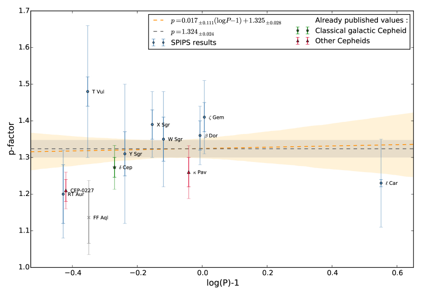
Figure 5: Relationship between the period and the $p$-factor for the Cepheids of our sample. We fitted both a constant (in black) and a linear regression (in orange). The error shades are defined by 1000 iterations of bootstrapping. The internal part of the error bar represents the statistical uncertainty. FF Aql is plotted in gray because it has not been used in the final adjustments.

In the results presented above, all the uncertainties have been determined after 1000 iterations of bootstrapping, which implicitly averages the errors on the single $p$ measurements (i.e., on the HST parallaxes), although this is not justified because of the probable correlation between these errors. To adopt a more conservative approach, we therefore could use the standard deviation of the residuals as a final uncertainty, which would lead to the following results (when excluding FF Aql from the adjustment): for the linear model, $p=0.017_{\pm 0.111}(\log P-1)+1.325_{\pm 0.085}$ and for the constant fit, $p=1.324\pm 0.084$.

6 Conclusion

We presented SPIPS models of the pulsation of nine Cepheids with available trigonometric parallaxes from Benedict et al. (2007). We deduce the values of their spectroscopic $p$-factor, and their IR excess (the signature of the presence of a CSE) and their color excess $E(B-V)$ (caused by interstellar reddening). Although the uncertainty of the parallaxes dominates the error bars on the derived $p$-factors, we conclude that within their total uncertainty, they are statistically consistent with a constant value independent of period, $p=1.324\pm 0.024$. The present calibration of the projection factor is limited by the relatively large uncertainty on the Cepheid parallaxes. As a result of the Gaia parallaxes that will be released over the next few years, we will soon be able to measure this essential parameter on a large sample of Galactic Cepheids with a sufficient accuracy to secure the PoP technique calibration at a 1% level. Although precise distances will be known for a large number of galactic Cepheids in the Gaia era, the SPIPS method will remain a very precious tool as it will lead to a better understanding of Cepheids physics (e.g., reddening, CSEs, etc.), essential for achieving the best precision and accuracy of the P-L relationships calibration. Thanks to the SPIPS method, we will also be able to measure the distance of extragalactic Cepheids and study the dependance with metallicity. A simultaneous use of the Gaia data and the SPIPS method will allow us to make a considerable step forward in the whole distance scale problematic.

Table 7: Best-fit output parameters given by the SPIPS code.

Name	Period (days)	p-factor	$\theta_{\rm{Ross}\leavevmode\nobreak\ \rm{at}\leavevmode\nobreak\ \phi=0}$ (mas)	$E(B-V)$	$<R>$ ($R_{\odot}$)	$<T_{\rm{eff}}>$ (K)	$V_{\gamma}$ (km/s)	$K$ excess (mag)	$H$ excess (mag)
RT Aur	$\bf{3.728305}$	$\bf{1.20}$	$\bf{0.6772}$	$\bf{0.048}$	$\bf{31.55}$	$\bf{5876}$	$\bf{19.65}$	$\bf{0.000}$	$\bf{0.000}$
	0.000005	$\leavevmode\nobreak\ \pm 0.08\leavevmode\nobreak\ \pm 0.09$	$\leavevmode\nobreak\ \pm 0.0025\leavevmode\nobreak\ \pm 0.0135$	$\leavevmode\nobreak\ \pm 0.008\leavevmode\nobreak\ \pm 0.016$	$\leavevmode\nobreak\ \pm 0.12\leavevmode\nobreak\ \pm 3.13$	$\leavevmode\nobreak\ \pm 23\leavevmode\nobreak\ \pm 50$	$\leavevmode\nobreak\ \pm 1.90\leavevmode\nobreak\ \pm 0.30$	$\leavevmode\nobreak\ \pm 0.006\leavevmode\nobreak\ \pm 0.020$	$\leavevmode\nobreak\ \pm 0.007\leavevmode\nobreak\ \pm 0.020$
T Vul	$\bf{4.435424}$	$\bf{1.48}$	$\bf{0.6071}$	$\bf{0.019}$	$\bf{35.39}$	$\bf{5736}$	see section 4	$\bf{0.004}$	$\bf{0.000}$
	0.000005	$\leavevmode\nobreak\ \pm 0.04\leavevmode\nobreak\ \pm 0.18$	$\leavevmode\nobreak\ \pm 0.0012\leavevmode\nobreak\ \pm 0.0120$	$\leavevmode\nobreak\ \pm 0.005\leavevmode\nobreak\ \pm 0.016$	$\leavevmode\nobreak\ \pm 0.07\leavevmode\nobreak\ \pm 4.98$	$\leavevmode\nobreak\ \pm 13\leavevmode\nobreak\ \pm 50$		$\leavevmode\nobreak\ \pm 0.001\leavevmode\nobreak\ \pm 0.020$	$\leavevmode\nobreak\ \pm 0.004\leavevmode\nobreak\ \pm 0.020$
FF Aql	$\bf{4.470848}$	$\bf{1.14}$	$\bf{0.8703}$	$\bf{0.167}$	$\bf{33.84}$	$\bf{5823}$	see section 4	$\bf{0.000}$	$\bf{0.000}$
	0.000010	$\leavevmode\nobreak\ \pm 0.07\leavevmode\nobreak\ \pm 0.07$	$\leavevmode\nobreak\ \pm 0.0014\leavevmode\nobreak\ \pm 0.0130$	$\leavevmode\nobreak\ \pm 0.007\leavevmode\nobreak\ \pm 0.016$	$\leavevmode\nobreak\ \pm 0.06\leavevmode\nobreak\ \pm 2.67$	$\leavevmode\nobreak\ \pm 21\leavevmode\nobreak\ \pm 50$		$\leavevmode\nobreak\ \pm 0.009\leavevmode\nobreak\ \pm 0.020$	$\leavevmode\nobreak\ \pm 0.009\leavevmode\nobreak\ \pm 0.020$
Y Sgr	$\bf{5.773383}$	$\bf{1.31}$	$\bf{0.8221}$	$\bf{0.205}$	$\bf{43.10}$	$\bf{5623}$	see section 4	$\bf{0.000}$	$\bf{0.011}$
	0.000009	$\leavevmode\nobreak\ \pm 0.06\leavevmode\nobreak\ \pm 0.18$	$\leavevmode\nobreak\ \pm 0.0027\leavevmode\nobreak\ \pm 0.0164$	$\leavevmode\nobreak\ \pm 0.007\leavevmode\nobreak\ \pm 0.016$	$\leavevmode\nobreak\ \pm 0.14\leavevmode\nobreak\ \pm 6.73$	$\leavevmode\nobreak\ \pm 19\leavevmode\nobreak\ \pm 50$		$\leavevmode\nobreak\ \pm 0.009\leavevmode\nobreak\ \pm 0.020$	$\leavevmode\nobreak\ \pm 0.009\leavevmode\nobreak\ \pm 0.020$
X Sgr	$\bf{7.012770}$	$\bf{1.39}$	$\bf{1.3157}$	$\bf{0.286}$	$\bf{48.37}$	$\bf{6117}$	$\bf{-13.15}$	$\bf{0.060}$	$\bf{0.034}$
	0.000012	$\leavevmode\nobreak\ \pm 0.04\leavevmode\nobreak\ \pm 0.08$	$\leavevmode\nobreak\ \pm 0.0023\leavevmode\nobreak\ \pm 0.0255$	$\leavevmode\nobreak\ \pm 0.004\leavevmode\nobreak\ \pm 0.016$	$\leavevmode\nobreak\ \pm 0.08\leavevmode\nobreak\ \pm 3.84$	$\leavevmode\nobreak\ \pm 15\leavevmode\nobreak\ \pm 50$	$\leavevmode\nobreak\ \pm 0.07\leavevmode\nobreak\ \pm 0.30$	$\leavevmode\nobreak\ \pm 0.004\leavevmode\nobreak\ \pm 0.020$	$\leavevmode\nobreak\ \pm 0.004\leavevmode\nobreak\ \pm 0.020$
W Sgr	$\bf{7.594984}$	$\bf{1.35}$	$\bf{1.1106}$	$\bf{0.029}$	$\bf{54.60}$	$\bf{5497}$	$\bf{-27.94}$	$\bf{0.106}$	$\bf{0.064}$
	0.000009	$\leavevmode\nobreak\ \pm 0.06\leavevmode\nobreak\ \pm 0.12$	$\leavevmode\nobreak\ \pm 0.0034\leavevmode\nobreak\ \pm 0.0170$	$\leavevmode\nobreak\ \pm 0.008\leavevmode\nobreak\ \pm 0.016$	$\leavevmode\nobreak\ \pm 0.17\leavevmode\nobreak\ \pm 5.63$	$\leavevmode\nobreak\ \pm 20\leavevmode\nobreak\ \pm 50$	$\leavevmode\nobreak\ \pm 0.04\leavevmode\nobreak\ \pm 0.30$	$\leavevmode\nobreak\ \pm 0.005\leavevmode\nobreak\ \pm 0.020$	$\leavevmode\nobreak\ \pm 0.020\leavevmode\nobreak\ \pm 0.020$
$\beta$ Dor	$\bf{9.842675}$	$\bf{1.36}$	$\bf{1.7767}$	$\bf{-0.018}$	$\bf{62.12}$	$\bf{5318}$	see section 4	$\bf{0.021}$	$\bf{0.000}$
	0.000019	$\leavevmode\nobreak\ \pm 0.04\leavevmode\nobreak\ \pm 0.07$	$\leavevmode\nobreak\ \pm 0.0024\leavevmode\nobreak\ \pm 0.0120$	$\leavevmode\nobreak\ \pm 0.005\leavevmode\nobreak\ \pm 0.016$	$\leavevmode\nobreak\ \pm 0.09\leavevmode\nobreak\ \pm 3.58$	$\leavevmode\nobreak\ \pm 12\leavevmode\nobreak\ \pm 50$		$\leavevmode\nobreak\ \pm 0.006\leavevmode\nobreak\ \pm 0.020$	$\leavevmode\nobreak\ \pm 0.005\leavevmode\nobreak\ \pm 0.020$
$\zeta$ Gem	$\bf{10.149806}$	$\bf{1.41}$	$\bf{1.6633}$	$\bf{-0.021}$	$\bf{64.87}$	$\bf{5326}$	see section 4	$\bf{0.000}$	$\bf{0.000}$
	0.000017	$\leavevmode\nobreak\ \pm 0.04\leavevmode\nobreak\ \pm 0.09$	$\leavevmode\nobreak\ \pm 0.0019\leavevmode\nobreak\ \pm 0.0491$	$\leavevmode\nobreak\ \pm 0.006\leavevmode\nobreak\ \pm 0.016$	$\leavevmode\nobreak\ \pm 0.08\leavevmode\nobreak\ \pm 6.12$	$\leavevmode\nobreak\ \pm 16\leavevmode\nobreak\ \pm 50$		$\leavevmode\nobreak\ \pm 0.007\leavevmode\nobreak\ \pm 0.020$	$\leavevmode\nobreak\ \pm 0.007\leavevmode\nobreak\ \pm 0.020$
$\ell$ Car	$\bf{35.551609}$	$\bf{1.23}$	$\bf{2.7805}$	$\bf{0.084}$	$\bf{159.01}$	$\bf{4696}$	$\bf{3.55}$	$\bf{0.000}$	$\bf{0.000}$
	0.000265	$\leavevmode\nobreak\ \pm 0.01\leavevmode\nobreak\ \pm 0.12$	$\leavevmode\nobreak\ \pm 0.0038\leavevmode\nobreak\ \pm 0.0283$	$\leavevmode\nobreak\ \pm 0.007\leavevmode\nobreak\ \pm 0.016$	$\leavevmode\nobreak\ \pm 0.21\leavevmode\nobreak\ \pm 17.44$	$\leavevmode\nobreak\ \pm 14\leavevmode\nobreak\ \pm 50$	$\leavevmode\nobreak\ \pm 0.04\leavevmode\nobreak\ \pm 0.30$	$\leavevmode\nobreak\ \pm 0.007\leavevmode\nobreak\ \pm 0.020$	$\leavevmode\nobreak\ \pm 0.005\leavevmode\nobreak\ \pm 0.020$

Appendix A SPIPS model for each Cepheid

The figures in this Appendix show the result of the SPIPS modeling of the stars of our sample (apart from $\ell$ Car, that is presented in Fig. 3). In all plots, the model is represented using a grey curve.