The Image Torque Operator for Contour Processing

Abstract

Contours are salient features for image description, but the detection and localization of boundary contours is still considered a challenging problem. This paper introduces a new tool for edge processing implementing the Gestaltism idea of edge grouping. This tool is a mid-level image operator, called the Torque operator, that is designed to help detect closed contours in images. The torque operator takes as input the raw image and creates an image map by computing from the image gradients within regions of multiple sizes a measure of how well the edges are aligned to form closed, convex contours. Fundamental properties of the torque are explored and illustrated through examples. Then it is applied in pure bottom-up processing in a variety of applications, including edge detection, visual attention and segmentation and experimentally demonstrated a useful tool that can improve existing techniques. Finally, its extension as a more general grouping mechanism and application in object recognition is discussed.

Keywords: Mid-level Vision; Image Operator; Segmentation; Object proposal

1 Introduction

Visual scene interpretation is very complex and involves computations at different levels of abstraction. Most theorists of vision adapt a categorization of visual processes and representations into low-, mid- and high-level vision [50]. The idea is that low level vision is about computing features, such as local edges, color, texture and image motion; mid-level vision groups local features to obtain object surfaces and global scene information, such as 3D motion and lighting; and high level vision utilizes semantic information to recognize objects, actions and scenes. The most influential ideas of mid-level vision are due to the Gestalt theorists. These psychologists of the early twentieth century [82] argued that human vision organizes image features at the early stages of interpretation through a process of figure ground segmentation. They suggested that certain principles are applied to group pieces of image and locate borders of figures. In this view, mid-level vision is about implementing organizational principles, such as similarity, symmetry, common fate (i.e. common motion), closure, bias from prior experience, etc., in order to identify the image regions which are object-related for further processing.

A very important cue of mid-level vision is the contour. Objects and parts of objects are delineated from their surroundings by closed contours, which make up their boundary. Many papers over the years have focused on contour detection [52, 24, 78], and there has been a renewed interest in recent years. A number of recent papers also have discussed mid-level cues and inspiration from Gestalt theory for contour processing in applications of detection [18, 36, 53], recognition [58, 44], and segmentation [3, 87]. These works mostly learn from data [65] to acquire mid-level representations. Here we pursue a very different approach; we propose a bottom-up mid-level mechanism for grouping edges into closed contours. Thus this mechanisms implements the so-called principle of closure, which refers to the idea that objects and object parts are perceived as whole, and simple features tend to be grouped together into closed figures even when they are not complete.

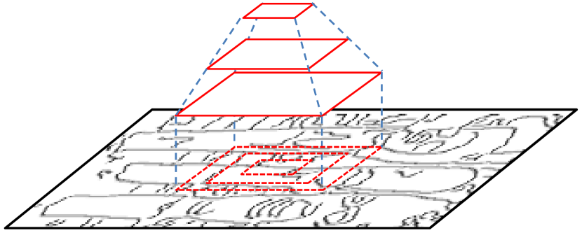
The grouping of edges is implemented with a semi-global image operator, which we call the torque operator. This operator is defined on oriented edges and provides a measure of the edge structure within a patch. It takes on large value when the patch contains a closed contour. The operator was designed as a tool to help detect regions likely to contain object or parts of objects. This is achieved by collecting edge information from regions of different extent in a way that enforces edges on convex contours and attenuates random edges due to texture. The torque within a patch is computed by taking at every edge point the value of the cross-product of the oriented edge and the vector from the center point of the patch, and summing over all values. To help the reader get a quick grasp of the basic idea, the concept is illustrated in Figure 1 before a proper definition of the operator will be given in Section 3.

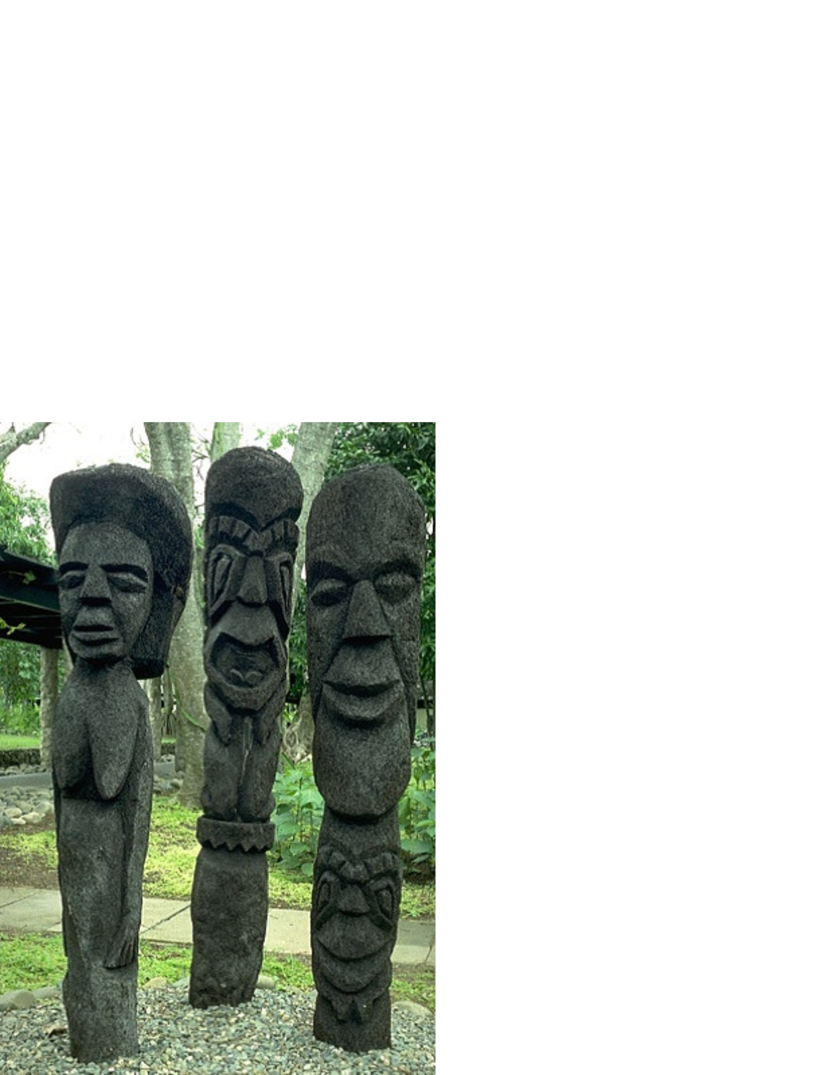
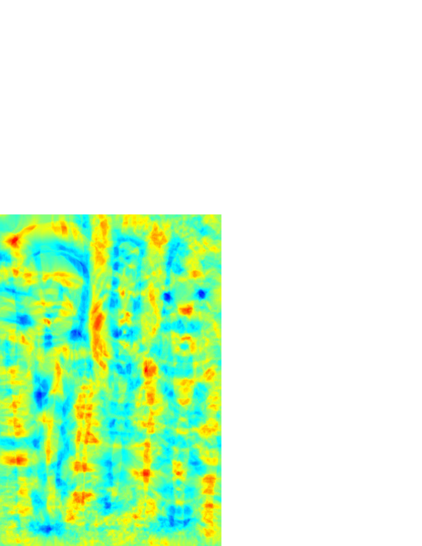
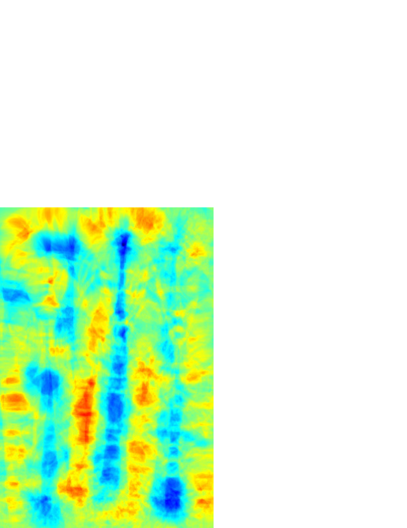
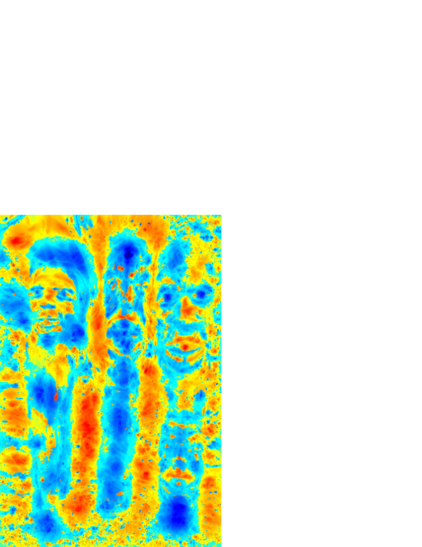
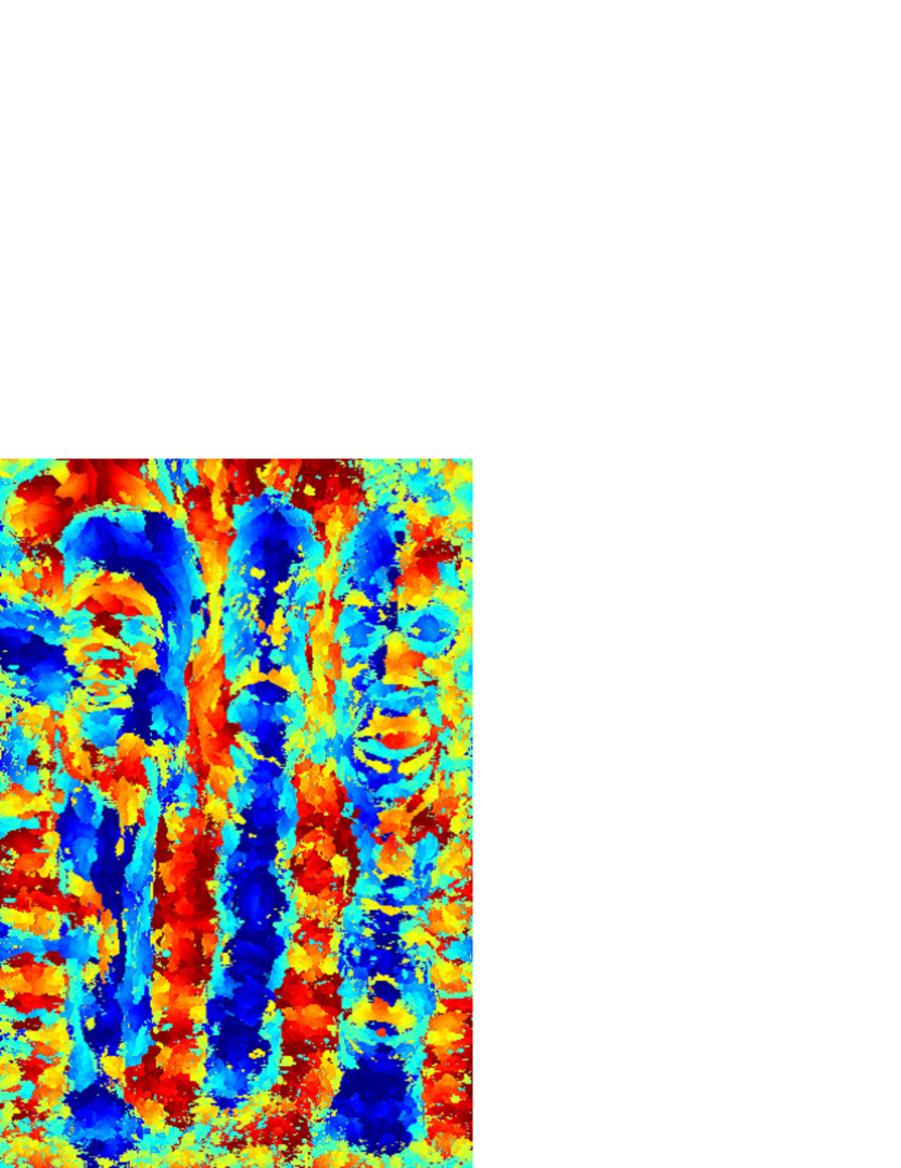
Referring to the figure, for the image on the upper left from the Berkeley data set [51], torque maps were computed for four different patch sizes ( $5\times 5$, $21\times 21$, $45\times 45$, and $81\times 81$ ). In these maps every pixel $p$ encodes the torque value from the patch of given size centered at $p$. We used the color coding as explained in the third row. Because edges are oriented, torque values can be positive (shown in red) and negative (shown in blue). We then define data structures: We call the three-dimensional structure of the torque maps at different scale the torque volume, and we combine the different scales into two-dimensional maps, which we call the torque value map and the scale map (as shown in the third row of Fig. 1). The torque value map at every pixel codes the value of largest absolute value over all scales, and the scale map codes the scale and the sign corresponding to the largest absolute torque value. These data structures will be used as tools to solve a number of applications.

5	21	45	81

Figure 1: Illustration of the torque. Upper row: left: Test image. right: Usage of the torque operator. The torque operator is applied to multi-scale image patches at every pixel in an image. Middle row: For the test image, examples of torque maps are shown for four patches of increasing size. Lower row: Combination of the torque at all patch sizes into one map, called the value map and the corresponding scale map.

The paper is organized as follows. After a description of related work in the next section, we provide a formal definition of the torque operator and discussion of its properties. Then we apply the torque operator in a few Computer Vision applications, specifically the problems of boundary detection, visual attention, segmentation, and object recognition, and we verify its usefulness as a tool that can improve existing techniques. Finally we conclude with a discussion on extending this operator to the spatio-temporal domain and as a grouping mechanism of high-level semantic edge information. Parts of this paper have previously appeared in [56].

2 Related Work

Contours are an essential cue for many vision applications, including segmentation, tracking and recognition. By the term contour, we generally refer to extended edges delineating objects and parts of objects. Already in the early days of Computer Vision it became clear that simple point-wise edge responses, computed with filters, are not sufficient to obtain salient edges corresponding to contours; some grouping mechanisms are necessary [61]. Earlier approaches employed semi-local edge-linking processes to obtain extended edges from edgels computed with local filters. For example, the well-known Canny edge detector traces edges using hysteresis thresholding. In more recent years the top performing algorithms employ edge detection methods specifically tuned to boundaries, and they use various linking and globalization processes, designed either for segmentation or recognition.

Boundary detection: Data-driven approaches to contour detection have been championed in the work of Martin et al. [52]. In this study, local cues, such as brightness, color, texture, and their gradients are combined, and weights for each cue are learned using labeled image data sets to distinguish edge points at boundaries from others. In similar spirit Dollár et al. [17] learn edge classifiers from simple features in image patches, Ren [63] combines information of local operators from multiple scales, and the high performance contour detection algorithm in [4] includes a globalization process to combine local edges based on the affinity of distant pixels. The latter method was further improved by Ren and Bo [64], who replaced the hand-selected features using patches obtained through sparse coding and dictionary learning, and integrated them through multi-scale pooling in the globalization. Zheng et al. [88] proposed an object-specific boundary detector by combining low-level information using the BEL edge detector [17] and foreground background cues, middle-level information about short and long-range connections of pixels, and high-level information from shape priors.

Recently Lim et al. [44] proposed an interesting generic mid-level detector, which they call sketch tokens. From patches of human-generated contours they learn different classes of edge features. Then using random forests, edge pixels are detected and classified as the center points of edge tokens. The approach was demonstrated in the bottom-up task of contour detection and the top-down task of object detection. In [18] a real-time algorithm for edge detection was proposed using the sketch tokens as features of structured information in a random forest [41]. This way edge detection is formulated as the prediction of local segmentation masks.

Over the years many computational models have been proposed for contour completion [21, 27]. For example in more recent work Kokkinos [38] first classifies boundary pixels based on SIFT features, and then groups the edge pixels using fractional linear programming based on the edge strength and a smoothness constraint, and Ren [63] linearly approximates edges and connects pixels using a conditional random field (CRF), which captures the statistics of continuity and different junction types. Most approaches to contour completion model the Gestalt rules of proximity and good-continuity. The principle of closure has also been proposed [21], for example in [68] for the task of segmentation. In recent work Ming et al. [53] used a higher-order CRF to model short and long range connections between edgels and junctions and implemented this way various edge completion principles, including the one of closure.

Most closely related to our work are the ideas of Lindeberg [45, 47] and Craft et al. [14]. In his seminal work on a computational theory of scale space, Lindeberg introduces, among other image feature detectors, the blob detector. Circular blobs in general can be detected using the Laplacian (or Difference of Gaussian) operator and scale space blobs are computed by filtering the image with scale-normalized Laplacians and detecting the local extrema in space and time. Lindeberg [46] also discussed the scale selection mechanism as a tool for selecting the focus of attention. The torque mechanism, introduced here, can be used in a similar way for attention selection, and if implemented with square windows or circular windows, has a very similar behavior. The torque, however, is more general. First, even if implemented with square (circular) windows, the torque value map can detect a larger range of shapes not just circular ones, and if used with differently shaped windows, it can also be tuned to certain structures. Secondly, we view the torque as a tool that can be used in many applications by using both the value and scale map.

Craft et al. [14] developed a computational neural model for figure-ground organization using a circular grouping mechanism. Their motivation was to provide an explanatory mechanism that can account for border-ownership and attention processes. At the first layer (modeling cells in area V1) oriented edge responses are computed and stored as pairs, one for each orientation. These cells are grouped in a second layer (modeling area V2) with top-down modulation from a third higher layer of larger-receptive cells, which tunes the grouping so it prefers annular patterns of different size (similar to a Laplacian filter). Our torque mechanism works in a similar way, but is more general. Instead of being tuned only to circular figures, the torque can group any closed figure, and it also has a scale selection mechanism. Craft et al. [14] proposed their model, not to solve Computer Vision applications, but to explain neurophysiological data. They also discussed physiological evidence in support of their biological model. Since the torque is a grouping mechanism for closure, it is linked to border-ownership and attention, and all of the arguments provided in [14] also apply to the torque mechanism. The most important ones are: Early edge signals involved in border-ownership representation code not only direction, but also orientation [80]. The speed of processing and size of fibers [89] indicate that border-ownership is not implemented through lateral connections, but rather requires a processing in higher order areas that feed back the signal. The processing time in border ownership signals was found not to dependent on the figure size. Finally, since figure-ground processes interact with higher-level processes, it must play a role in visual attention selection, and the two processes must be closely related. Our torque mechanism has all these features: (a) it uses orientation of edges; (b) is an additional mechanism (higher level than edge-linking) which can feed back to simple edges; (c) as a scale-space mechanism its computation does not depend on the size of object, and (d) it lends itself naturally as a tool for attention selection.

Segmentation: The fundamental approach to segmentation is to separate surfaces, assuming that individual surfaces are homogeneous in some local measurements, such as color intensity, texture [2, 69, 6], motion [15, 86, 57, 23] or depth [40, 83], and neighboring surfaces are separated by discontinuities in these cues. We here differentiate between approaches that treat segmentation as the problem of dividing the image into multiple regions, and approaches that consider the problem as separating one foreground object from background. Examples of the former are the mean-shift method [13] and graph-partitioning methods using the graph cuts algorithm [9] or the normalized cut approach [69]. These segmentation approaches are usually based on local cues as input to a global optimization, but recently many methods first compute super-pixels [62, 37] by over-segmenting the image into perceptual uniform regions based on the statistics in neighborhoods or affinity between points.

Approaches that consider foreground-background segmentation include probabilistic models that formulate the problem as optimization for a binary labeling and use belief propagation or graph cut algorithms [67, 40] and continuous models based on differential equations using methods such as active contours and variational approaches [7, 55, 59]. Our evaluation here uses graphcut methods. We use the classical graphcut segmentation into multiple segments [10] and the foreground-background separation approach of [54]. The latter method segments in the polar coordinate system by minimizing for a closed contour surrounding a fixation point using a graph cut formulation defined on edges only. All segmentation approaches have the problem of being biased, usually towards small regions with small and smooth boundary. This is because of texture edges, which in real images are always present, in conjunction with minimizations biased towards certain shapes. For example graph cuts [40] are known to favor small areas, the polar coordinate representation favors circular blobs, and variational minimizations [79] also prefer smaller segments, as they explicitly minimize the length and/or smoothness of the bounding contour. By using the torque in a preprocessing step to find object-like regions, it can alleviate the bias. It can help locate the regions surrounded by contours, locate contours of larger extent, and separate texture edges from boundary edges.

Visual attention: Attention mechanisms are classified into bottom-up and top-down processes. Top-down attention is more complex because it represents objects in memory [29] and uses the memory to detect likely objects in an attended visual scene. Bottom up attention is driven by low level processes. The best known model of visual attention has been proposed by Itti et al. [32]. In this model, first local feature maps are computed from color, intensity and orientation information as the difference of Gaussian filters at multiple scales, which approximate the center-surround differences of neurons. Larger center surround differences are considered more conspicuous. Then a combined saliency map is constructed by adding the normalized feature maps. Related approaches differ in the choice of feature vectors and combination of features. In our experimental section we will compare against the method of Harel et al. [28], which computes a saliency map based on the dissimilarity of features in regions using a graph-based approach. Harel et al. evaluated the performance of their detector on its ability to predict human attention using the human fixation data of Einhäuser et al. [20], and reported to achieve 98% of the ROC area of a human based control, while the model by Itti et al. achieved only 84%. Recent works in fixation and attention [30, 19] offer an alternative to the traditional early feature saliency theories. Based on systematic psychophysical experiments, [30] suggests that observers look at objects as if they knew them before they became aware of their identity, and [19] shows that the hypothesis that humans attend to objects has a better predictive power in the data than any other theory. A number of works recently proposed algorithms for the implementation of this idea calling it proto-segmentation and object proposal [1, 12, 31]. In our paper we will use the torque measure to derive a saliency map for visual attention. The extrema of the torque measure often appear at the locations in the image where objects are surrounded by edges. Thus the torque appears to be a good measure to model object driven visual attention.

Object recognition: The best known object recognition methods use descriptors based on point detectors tuned to texture features [48, 16], but object recognition from contours has also received significant attention. We can roughly classify existing approaches according to how they detect and describe local contour features and how they represent and classify the overall contour. Often, so-called contour patches, or shape fragments, are used as local descriptors. For example, the shape context descriptor [5] encodes the spatial distribution of edge points in log polar space, or the feature detector defined by [35] is based on the saliency of local convexity. Some approaches acquire the contour fragments and their detectors [42, 70, 58, 43, 49] from data using learning techniques. For, example Shotton et al. [70] and Opelt et al. [58] learn a codebook of shape fragments. To detect objects, the learned class specific shape fragments are then matched using oriented chamfer matching and voted via a star-shape model. Leibe et al. [43] encode with the patches the relative location to the object center, to create a codebook that in addition to appearance also represents spatial information for particular object classes. For a better representation of object classes, some techniques group contour pieces into longer lines and curves [24, 60] and match object parts. A descriptor for matching partial shape fragments was introduced in [66], and Toshev et. al. [77] proposed the chordiogram descriptor to encode relative angles of boundary segments. Our contribution to recognition here is a contour-based patch detector and a patch descriptor. The contour patch detector is based on extrema in the torque map, and the contour patch descriptor is is based on the torque values in the detected patch at multiple scales. We then use a simple bag-of-word representation and an SVM for object classification.

3 Torque Operator

After providing a definition of the torque operator, we discuss its properties that make it useful for contour processing. Then we provide the data-structure for representing the torque, illustrate its application on various examples, and discuss issues related to scale selection. Finally, we provide an efficient implementation of the torque using the so-called integral images.

3.1 Definition

Torque, as defined in physics, is the tendency of a force to rotate an object about an axis. Mathematically, torque is defined as the cross product of the force and the displacement vector from the point at which torque is measured to the point to which the force is applied, as depicted in Fig. 2:

$$\vec{\tau}=\vec{r}\times\vec{F},$$ (1)

where $\vec{\tau}$ is the torque vector, $\vec{r}$ is the displacement vector, and $\vec{F}$ is the force vector.

To define a torque measure for images, we consider forces applied at edge points and parallel to the tangent of the local edge. For an arbitrary point, called the center point, we consider a rotation axis in three-dimensional space passing through that point and perpendicular to the image plane. Then we can measure the torque at any point in the image with respect to the rotation axis, as defined in physics (see Fig. 2). Since the displacement vector and the force vector are both on the image surface, the torque vector is perpendicular to the image surface, and we call the magnitude of the torque vector along the rotation axis simply the torque or torque value here and after.

\begin{overpic}[width=301.36906pt,keepaspectratio={true},clip]{ImageTorqueIdea.eps} \put(154.0,39.0){$p$} \put(164.0,35.0){$\vec{r}$} \put(188.0,35.0){$\vec{F}$} \put(163.0,69.0){$\vec{\tau}$} \put(11.0,27.0){\rotatebox{53.0}{\tiny displacement}} \put(28.0,22.0){\rotatebox{-25.0}{\tiny force}} \put(44.0,72.0){\tiny torque} \end{overpic}

Figure 2: The idea of the image torque measure is inspired by the concept of the torque in physics: Given a point $p$ and an edge point $q$ in an image, we assign a unit force vector $\vec{F}$ along the tangent of the edge. Denoting as $\vec{r}$ the vector from $p$ to $q$, the torque vector at $q$ is defined as $\vec{\tau}=\vec{r}\times\vec{F}$. Its value along the axis perpendicular the image will be called the torque.

Since our images are discrete, edges are represented by a set of pixels. Let $q$ be an edge point, whose edge we represent by a vector $\vec{F}_{q}$, and let $p$ denote the center point and $\vec{r}_{pq}$ the displacement vector from $p$ to $q$. Then the torque value at $p$ is

$$\vec{\tau}_{pq}=\vec{r}_{pq}\times\vec{F}_{q}.$$ (2)

With slight abuse of notation, here the cross product of two-dimensional vectors denotes the scalar obtained by cross-multiplying the vectors. If we further assume the force vector of unit length, the value of the torque amounts to:

$$\tau_{pq}=\left\|\vec{r}_{pq}\right\|\sin\theta_{pq}.$$ (3)

Note that in our definition edges are oriented, where the orientation is defined by contrast. Thus, the value of the torque can have positive and negative values. We define the orientation of an edge as perpendicular clockwise to the image gradient, such that the brighter side is on its right and the darker side on its left.

We then define an image operator on local image patches. The torque operator is defined as the sum over the torque values of all edge points within an image patch of arbitrary shape. Applying the torque operator, $\tau_{P}$, to a patch we obtain the torque of an image patch as:

$$\tau_{P,p}=\frac{1}{2\left|P\right|}\sum_{q\in E\left(P\right)}\tau_{pq},$$ (4)

where $E\left(P\right)$ is a set of edge points in the patch $P$, and $p$ is the center point of the patch. $\left|P\right|$ is the area of the patch, which is used for normalization to achieve independence of the patch size. This will become clear in the next section, where it is shown that the torque of a patch is related to the area under the curve.

We apply the torque operator over the entire edge map, shifting the position of the patch and varying the size of the patch as depicted in Fig. 1. In principle, the shape of the patch could be arbitrary, but in this paper we will use disk or square patches for illustration (Sec. 3), and square and rectangle patches in our efficient implementation and the experiments (Sec. 4).

3.2 Properties of Torque Operator

Next some of the basic properties of the torque operator are explained to motivate the usefulness of the torque in different applications.

3.2.1 Torque and Area

Since the torque is defined by the cross product of vectors, it is essentially related to the area defined by these vectors as shown in Fig. 3. This relationship can be easily extended to edge curves. Assuming edges are clean continuous curves, the value of the torque in a patch is related to the position of the curves in the patch and their shape. For curve segments intersecting the boundary of the patch with center $p$ at two intersection points $q_{1}$ and $q_{2}$ as in Fig. 4(a), the torque is proportional to the area enclosed by the edge curve and the two line segments $\overline{pq_{1}}$ and $\overline{pq_{2}}$. The torque of a closed curve, completely inside the patch, is proportional to the area under the curve (Fig. 4 (b)). The closer the curve to the patch boundaries, the larger the torque of the image patch. We normalize for the patch size, so we can compare the torque across scales. Intuitively, it then can be understood that the torque operator can be useful for finding the scale of closed curves.

\begin{overpic}[width=225.91432pt,keepaspectratio={true},clip]{TorqueAreaColor.eps} \put(42.0,17.0){$p$} \put(60.0,10.0){$\vec{r}$} \put(105.0,14.0){$\vec{F}$} \put(40.0,45.0){$\vec{\tau}$} \put(70.0,20.0){\scriptsize{$\frac{1}{2}\left\|\vec{r}\times\vec{F}\right\|$}} \end{overpic}

Figure 3: Cross product and area. The triangle enclosed by vectors $\vec{r}$ and $\vec{F}$ is equivalent to $\left\|\vec{r}\times\vec{F}\right\|/2$.

\begin{overpic}[width=433.62pt,keepaspectratio={true},clip]{TorqueAreaPartial.eps} \put(35.0,30.0){$p$} \put(70.0,50.0){$q_{1}$} \put(70.0,20.0){$q_{2}$} \end{overpic}	\begin{overpic}[width=433.62pt,keepaspectratio={true},clip]{TorqueAreaFull.eps} \put(35.0,30.0){$p$} \end{overpic}
(a)	(b)

Figure 4: Relationship between torque and area. Two cases are shown: (a) the disk patch is smaller than the object, and it covers only a part of the boundary; (b) the disk patch covers the whole object boundary.

3.2.2 Texture vs Boundary

An important function of the torque as a mid-level operator is to separate aligned edge structures from random texture edges. The torque of a patch will be larger when the patch has long contours and it will be largest if the edges are structured into closed contours. On the other hand, the torque is expected to be small when the edges are due to random texture as illustrated in Fig. 5. This is, because in our definition of the torque, edges have an orientation defined by the contrast. Therefore, in textures (made up of blobs and textons) where oriented edges in the patch appear in pairs, they cancel each other. Assuming there is sufficient randomness in the edge distribution, the sum of contributions will be small.

	\begin{overpic}[width=433.62pt,keepaspectratio={true},clip]{TorqueValueMap_texture.eps} \put(5.0,12.0){Max torque} \put(20.0,2.0){0.39} \end{overpic}		\begin{overpic}[width=433.62pt,keepaspectratio={true},clip]{TorqueValueMap_boundary.eps} \put(5.0,12.0){Max torque} \put(20.0,2.0){0.79} \end{overpic}
(a)	(b)	(c)	(d)

Figure 5: Torque on texture edges and boundary edges. The maximum absolute torque value (over all patch sizes) tends to be small for random texture edges (a and b) and large for closed boundaries (c and d).

3.2.3 Extrema in Torque

The torque tends to be large in magnitude if the patch contains extended contours close to the boundaries of the patch. Therefore, it is expected that the torque measure is useful for finding the locations in the image where edges are in structure forming closed contours. Furthermore, the torque can give us the scale of the region of those structured edges. This concepts is illustrated in Figure 6 for an example where the structured edges form a triangle. The figure shows the torque value maps for four sizes, and graphs the torque values at the center of the triangle over all patch sizes. As can be seen, the location of structured edges, i.e. the triangle, can be inferred from the maximum of the torque over space and patch sizes. The patch size of the torque maximum indicates the size of the triangle.

Next we formally define the data-structures used in the torque computation, then we provide further examples illustrating the torque value on real objects of different shape.

	2	10	21	30

\begin{overpic}[width=433.62pt,keepaspectratio={true},clip]{TorquePlotTriangle.eps} \put(5.0,0.0){$0$} \put(31.0,0.0){$5$} \put(56.0,0.0){$10$} \put(83.0,0.0){$15$} \put(109.0,0.0){$20$} \put(135.0,0.0){$25$} \put(163.0,0.0){$30$} \put(50.0,-8.0){Patch Radius (Scale)} \put(-5.0,5.0){$0.0$} \put(-5.0,23.0){$0.1$} \put(-5.0,41.0){$0.2$} \put(-5.0,59.0){$0.3$} \put(-5.0,77.0){$0.4$} \put(-5.0,95.0){$0.5$} \put(-13.0,40.0){\rotatebox{90.0}{Torque}} \end{overpic}

Figure 6: First row: Torque maps for a triangle for different patch sizes. The numbers below the torque maps denote the radius of the disk patch in pixels. Second row: Torque values at the center of the triangle shown over patch sizes.

3.3 Representation of the Torque

By applying the torque operator to an image using a single patch size, we obtain a two-dimensional map of torque values. Applying the torque operator using multiple patch sizes, we obtain multiple maps at different scale (see Fig. 1). The set of maps at different scales makes a three-dimensional volume. However, it is often convenient for applications to combine the maps at different scales into two dimensional maps, $V$ and $S$, which we describe by the following equations:

$$V\left(x,y\right) =\tau\left(x,y,\hat{s}\left(x,y\right)\right),$$ (5)

$$S\left(x,y\right) =\operatorname{sgn}\left(V\left(x,y\right)\right)\cdot\hat{s}\left(x,y\right),$$ (6)

$$\hat{s}\left(x,y\right) =\operatornamewithlimits{argmax}_{s}\left|\tau\left(x,y,s\right)\right|.$$ (7)

$\tau\left(x,y,s\right)$ is the torque value at point $\left(x,y\right)$ with patch size (scale $s$). We call the three-dimensional volume of $\tau$ the torque volume, and $V$ and $S$ the torque value map and scale map, respectively.

Figure 7 shows examples of torque value maps and scale maps for some simple figures. As can be seen the torque operator captures well the concept of closure. For these simple shapes, the torque value map directly provides the location of the object, i.e. the center of the polygon, and the scale map provides its scale (at the point corresponding to the extrema in the value map).

The torque maps are more complex for multiple objects located close to each other, or for objects of different topology. Figure 8 illustrates the theoretical and empirical maps for two situations: the case of an object on top of another object, and the case an object with a hole. The former is illustrated for two dark objects on bright background with the object at the bottom darker than the one on top. The object regions have negative torque value, but positive torque values appear on the brighter object around the edges shared with the darker object. This is because the edge orientation is defined by polarity. In this region the edge boundary abuts a darker region, which is in conflict with the other edges which abut brighter regions. Thus, these edges give torque values of opposite sign, and result in a positive torque value region close to the edge. For the case where the object has a hole, we do not have such a confusion.

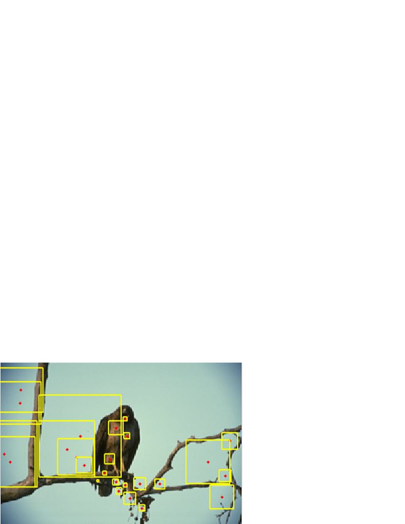
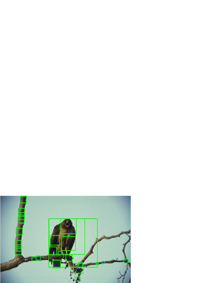
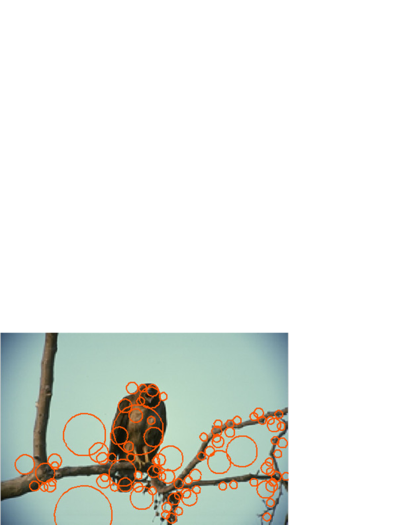
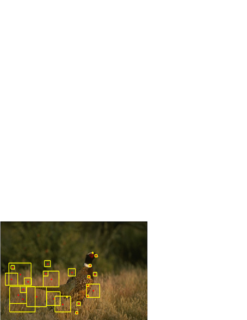
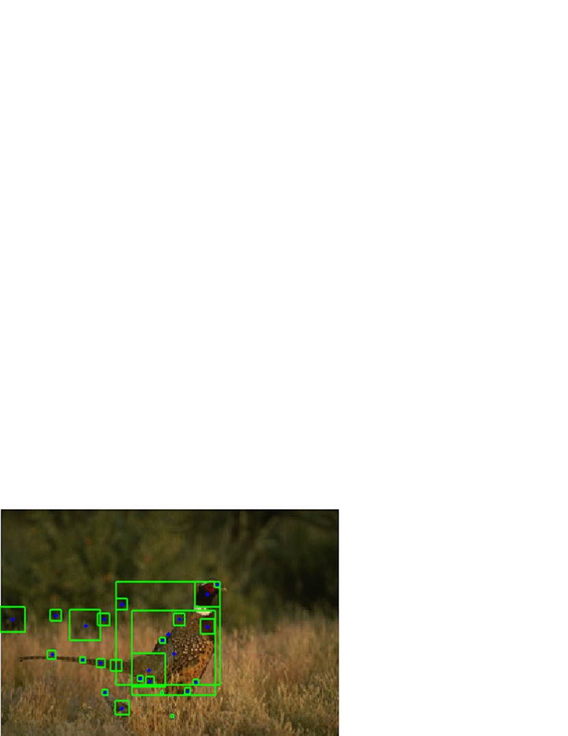
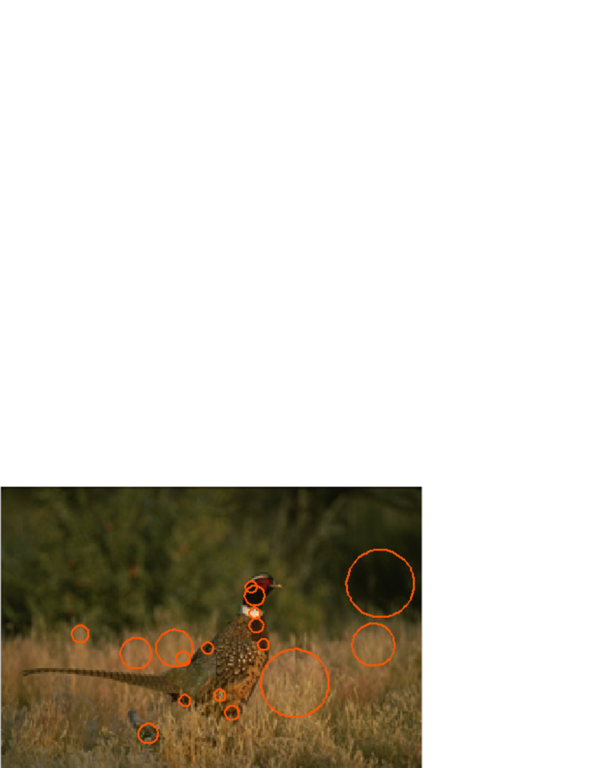
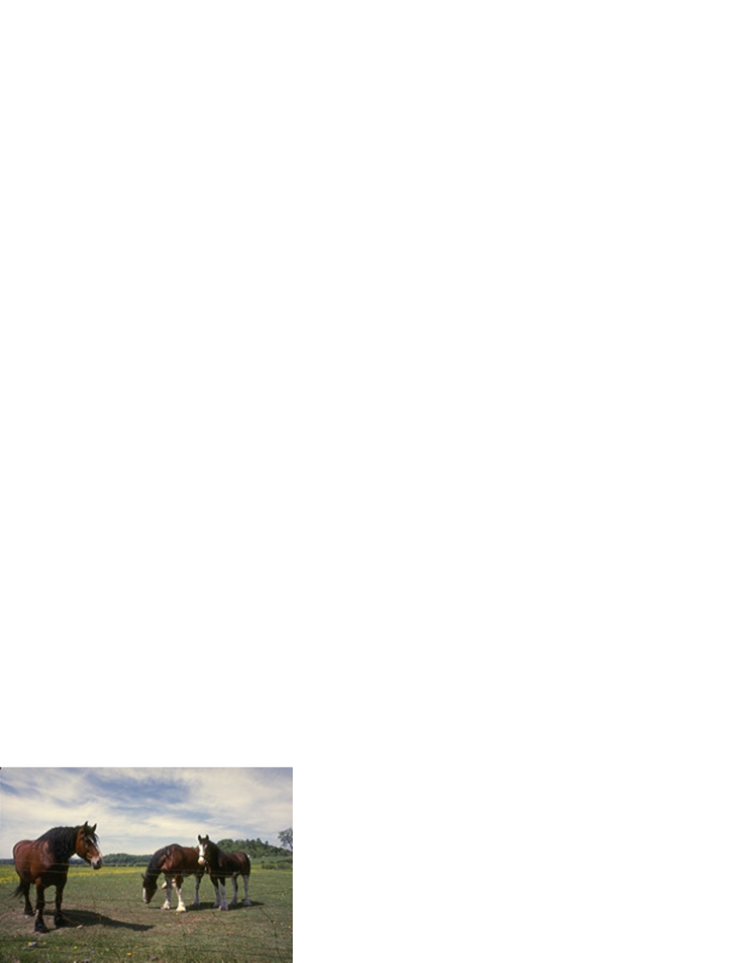
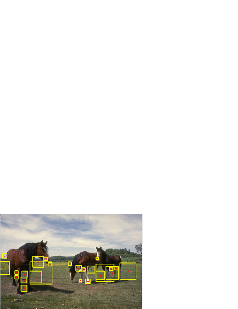
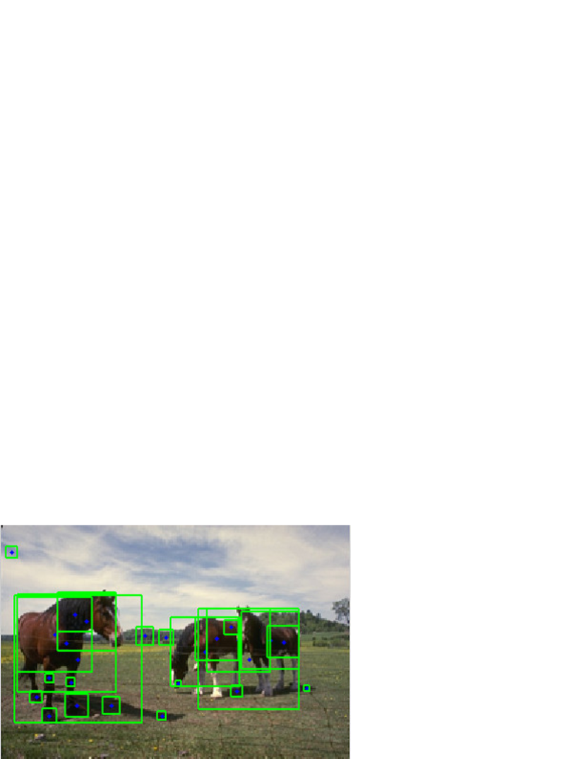
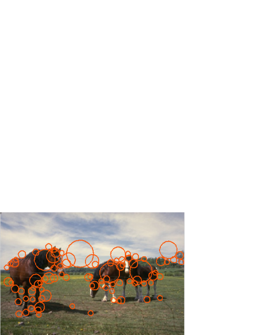
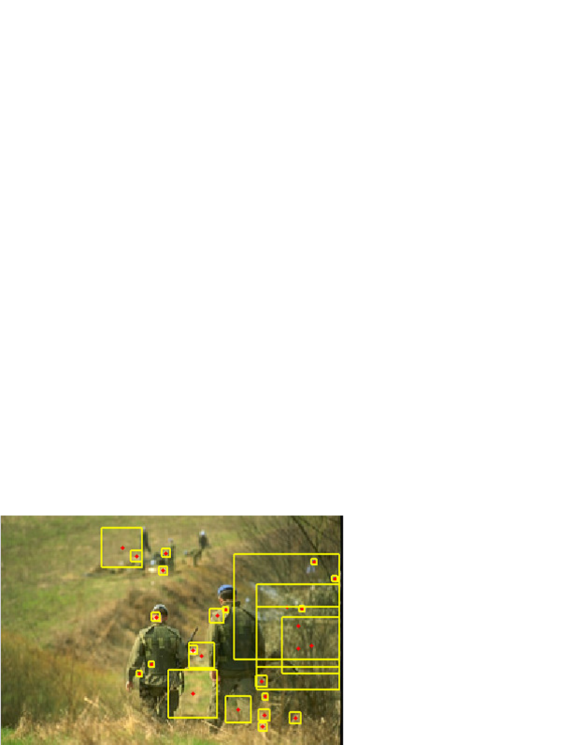
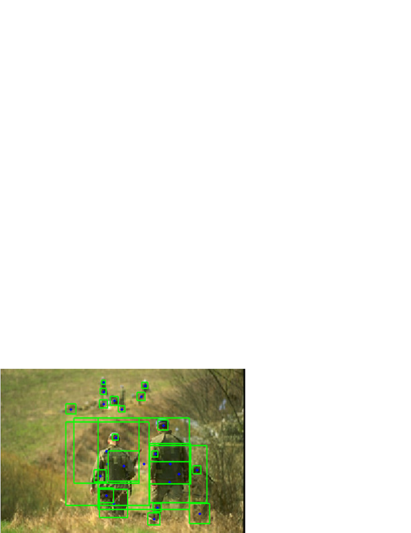
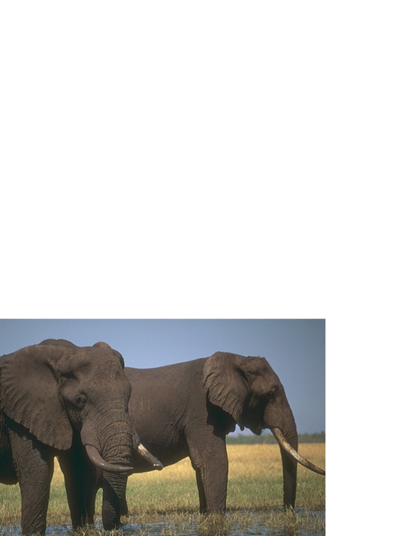
Figure 9 illustrates the application of the torque operator on real images from the Berkeley dataset [51]. Here square patches were used with their sizes varying from 3 to 91 pixels, and the images were downsized by a factor of two to $161\times 241$. Thus the largest image patch covers about 21% of the image area. Figures 9 (a)- (d) show the test images, torque value maps, and location of the extrema and corresponding patch sizes (as green squares for minima and yellow squares for maxima). For each test image, the 25 maxima and 25 minima of largest absolute torque values are shown (in 9 (c) and (d), respectively). As can be seen from column (b), the negative torque regions match well object regions for these images. We should note that the sign of the torque depends on the relative brightness of an object to the background, and in all these examples the objects are darker than their surroundings (as reflected in the torque minima in column (d)). An interesting property of the torque operator is that the extrema are not located simply at the dense edges, but at locations surrounded by edges. For example, in the image of the pheasant, the inner part of the pheasant doesn’t have clear edges. Nevertheless, local minima are found in the torque volume, and the location of structured, surrounding boundaries in these parts are detected. A second interesting property of the torque operator is that the extrema indicate the size of structured edges. Referring to the figure, it can be seen that the patches associated with local minima (shown in green) cover most of the object regions. These properties of indicating roughly the location and size of structured edges are useful for further image processes, such as visual attention and object segmentation.

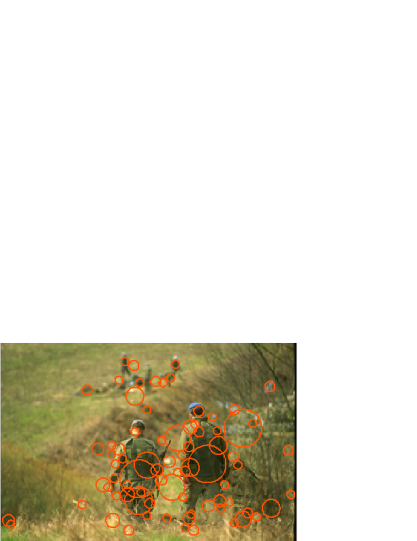
Fig. 9(e) provides a comparison to the blob detection of [47] using the implementation in [39]. The blob detector locates the points in scale space where the square of a normalized Laplacian assumes maxima with respect to space and scale. The extrema are thus contrast invariant (i.e, both dark blobs on light background and light blobs on dark background). The torque extrema also amount to local extrema with respect to space and scale, but we separate them according to contrast. Comparing visually the blob detection to the torque minima, we can see that the latter tends to have extrema representing whole objects. We can see that the regions of the eagle, the pheasant, the horses, and the persons are detected by negative torque extrema in the test images. This indicates that the torque detector has greater flexibility to shape variation. The blob detector is maximally tuned to annular-like image patches (like the Laplacian kernel). The torque detector, if implemented with square or disk windows, also is maximally tuned to circular structures, but it also responds to other shapes, especially closed convex shapes, as it adds up all the edgels in the window. Furthermore, we see the torque mechanism as a more general concept, and it can be extended in various ways. For example, we can use other window shapes, as in section 4.4, or we can also tune it to favor certain shapes. Furthermore, besides the extrema, we can also utilize the torque values and scales, as in Section 4.4.

Figure 7: Torque value maps (upper row) and scale maps (lower row) for simple shapes. The shapes are overlaid onto the torque value with black lines. Black regions in the scale map denote areas where the torque value is the same over scales.

Figure 8: Torque for two configurations with multiple objects. The first row shows graphical examples of the configuration, and the second row shows real images with objects of such configuration. Columns (1 and 4), (2 and 5) and (3 and 6) show the test images, the scale maps and torque value maps, respectively.

(a)	(b)	(c)	(d)	(e)

Figure 9: Torque value maps and extrema in torque. (a) Original test images. (b) Torque value maps. (c) and (d) Local maxima and local minima in torque volume, respectively. Dots indicate the location of extrema in image space, and the corresponding squares indicate the size of the patch producing the extrema. (e) Blob detection [47, 39] as reference.

3.4 Scale Selection

In the previous section we proposed a two-dimensional representation of the torque volume as torque value map and scale map. The torque value map and scale map are generated from the torque volume by selecting at each pixel the scale corresponding to the largest absolute torque value over scales. Scale selection in general is an important topic in computer vision [45, 47], and selecting the appropriate scale can lead to better performance in most image processing tasks [25, 84].

Our main focus in this paper is detection of object-like structures, and thus for most images we want to avoid attention to smaller structures. One strategy to handle this within the torque framework, is to first reduce the noise in the torque volume due to edge fragments and then select the scale. Standard techniques for noise reduction such as filtering and optimization can be applied to the torque volume.

Another way to modify the scale selection is by modifying the normalization factor. This is motivated by the work of Galun et al. [25], who studied the ideal threshold for multi-scale edge detection under Gaussian noise assumptions. The torque for a patch is defined (from eq. 4) as:

$$\tau_{P,p} =\frac{1}{2Z}\sum_{q\in E\left(P\right)}\tau_{pq},$$ (8)

where $Z$ is the normalization factor, and it was set to $|P|$, i.e. the area of the patch in eq. (4). For a disk patch of radius $R$ it amounts to $|P|=\pi R^{2}$. We now vary the normalization factor by introducing a parameter $\alpha$ as follows:

$$Z =\pi R^{\alpha}.$$ (9)

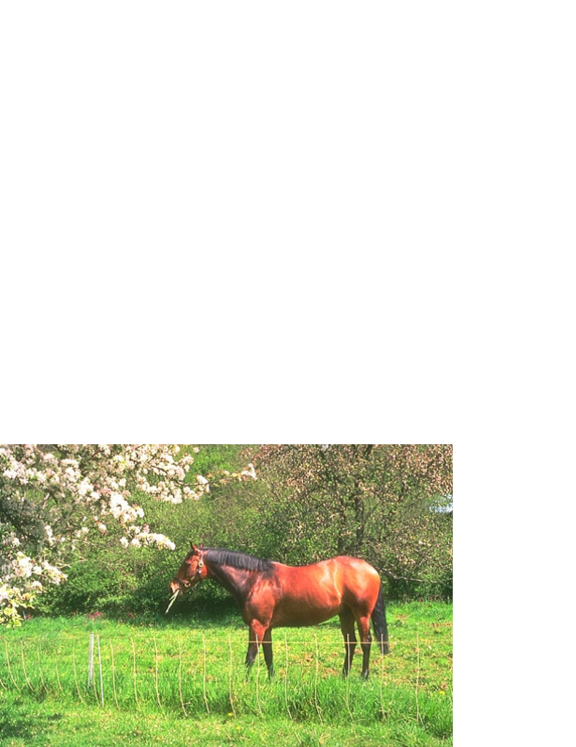
Fig. 10 shows torque value maps for different $\alpha$ values. As can be seen from the figure, the torque value maps become smoother as $\alpha$ gets smaller. This is because image patches of larger size now have a smaller normalization factor, and therefore they tend to produce relatively higher torque values. As a result larger edge structures get favored. Thus, a smaller $\alpha$ gives the effect of smoothing the torque value maps. An $\alpha=1$ corresponds to a normalization by the square root of the patch area, which is also the ideal normalization of the area term derived by [25] for edge multi-scale detection. In general, the amount of smoothing preferred will depend on the application, and by adjusting the normalization factor, $\alpha$, one can easily adapt the torque operator.

Test Image	$\alpha=1.0$	$\alpha=1.5$	$\alpha=2.0$
(a)	(b)	(c)	(d)

Figure 10: Torque value maps with different normalization factors. (a) Test images; (b)-(d) torque value maps corresponding to the normalization factor $\alpha$ shown at the top of each column. As $\alpha$ gets larger, the number of positive and negative regions in the torque value map increases.

3.5 Efficient Torque Computation

The computation of torque would be time consuming with a straightforward implementation. However, the torque can be computed efficiently using the concept of integral images, which will be explained next. A then discusses a slightly modified torque definition, which allows for a very efficient computation.

First, let us quickly review the concept. An integral image (or summed area table) is a data-structure and algorithm to generate the sum of values in rectangular areas of an image. Let $k(x,y)$ be some image quantity. The value $K(x,y)$ for the region of pixels in the range $[0\dots x,0\dots y]$ amounts to

$$K(x,y)=\sum_{u\leq x}\sum_{v\leq y}k(x,y),$$ (10)

and it can be computed in a single pass over the image as

$$K(x,y)=k(x,y)+K(x-1,y)+K(x,y-1)-K(x-1,y-1).$$ (11)

Once the table has been created, the sum of values in any rectangular region $[a\dots b,c\dots d]$ can be computed in constant time with only one addition and two subtractions as:

$$\sum_{u=a}^{b}\sum_{v=c}^{d}k(u,v) = K(a,c)+K(b,d)-K(a,d)-K(b,c).$$ (12)

Let us now explain how to use these concepts to compute the torque. Let $o$ be the origin of the image coordinate system in the left top corner of the image, and let $p$ be the center of a patch $P$, and $\overrightarrow{F_{q}}$ the edge vector at $q$. We emphasize that now we need to change the center with respect to which we compute the torque, which is denoted as subscript in our notation. Using a vector notation, the torque of the patch $P$ with respect to center $p$ without normalization can be written as:

$$\vec{\tau}_{P,p}\cdot(2\left|P\right|) = \sum\limits_{q\in P}\overrightarrow{pq}\times\overrightarrow{F_{q}}$$ (13)

$$= \sum\limits_{q\in P}(\overrightarrow{po}+\overrightarrow{oq})\times\overrightarrow{F_{q}}$$

$$= -\overrightarrow{op}\times\sum_{q\in P}{\overrightarrow{F_{q}}}+\sum_{q\in P}{\overrightarrow{oq}}\times{\overrightarrow{F_{q}}}.$$

The first term in eq. (13) amounts to the cross-product of the vector from the origin to $p$ and the vector of the sum of edges in the patch. The second term is the torque computed with respect to the origin of the image. If we express the vectors in terms of their components to denote $\overrightarrow{op}=(x,y)$, $\overrightarrow{oq}=(u,v)$ and $F_{q}=(F^{x}(u,v),F^{y}(u,v))$, we can rewrite eq. (13) as

$$\vec{\tau}_{P,p}\cdot(2\left|P\right|) =$$

$$\left.-x\sum_{\left(u,v\right)\in P}F^{y}\left(u,v\right)+y\sum_{\left(u,v\right)\in P}F^{x}\left(u,v\right)\right.$$

$$\left.+\sum_{\left(u,v\right)\in P}uF^{y}\left(u,v\right)-\sum_{\left(u,v\right)\in P}vF^{x}\left(u,v\right)\right.$$ (14)

Now it becomes clear that for each of the terms $F^{x}$, $F^{y}$,$uF^{y}$ and $vF^{x}$ we can pre-compute summed area tables with respect to the origin, and then compute the values for any patch in linear time to derive the torque of the patch.

Further efficiency in the torque computation can be obtained by approximating the edge orientation to one of equally divided eight directions:

$$\theta_{i}=\left(i-1\right)\frac{2\pi}{8},$$ (15)

where $i\in\left\{1,2,3,4,5,6,7,8\right\}$ is the index to the orientation. An edge vector of orientation $\theta_{i}$ is represented by a unit vector $\left(\cos\theta_{i},\sin\theta_{i}\right)$. The torque at a point $q=(x,y)$ with respect to center $o$ for an edge vector in orientation $i$ then amounts to

$$\tau_{oq}(i) =(x\sin\theta_{i}-y\cos\theta_{i})\cdot\delta\left(q,i\right),$$ (16)

where $\delta\left(q,i\right)\in\left\{0,1\right\}$ is a binary indicator for the existence of an edge at pixel $q$ in the orientation indicated by $i$, and the torque at point $q$ is:

$$\tau_{oq} =\sum^{8}_{i=1}\tau_{oq}(i).$$ (17)

With this approximation, the torque in an image patch before normalization in eq. (13) becomes

$$\vec{\tau}_{P,p}\cdot(2\left|P\right|)=$$

$$\left.\sum^{8}_{i=1}\left((-x\sin\theta_{i}+y\cos\theta_{i})\sum_{\left(u,v\right)\in P}\delta\left((u,v),i\right)\right)\right.$$

$$\left.+\sum^{8}_{i=1}\sum_{\left(u,v\right)\in P}\tau_{o}((u,v),i)\right.$$ (18)

We then implement the torque by keeping two three-dimensional arrays, one to store the edges, represented as $\delta\left(x,y,i\right)$, and one to store the torque values $\tau\left(x,y,i\right)$, and we compute summed area tables for each $\delta\left(x,y,i\right)$ and $\tau\left(x,y,i\right)$. The computational cost is independent of the patch size. For any given patch size, computing the torque for all patches in the image is linear in the number of pixels $N$, i.e. $O\left(N\right)$.

Finally, let us look at the computational efficiency of the Torque operator and compare it to common approaches. The well-known SIFT algorithm involves two steps: detection of key points and generation of a description. The key point search in SIFT, which is like blob detection, has similarity to the extrema detection in the torque volume as both are multi-scale localization procedures of interest points. As analyzed in [26], the highest costs in the key point search in SIFT are due to the multiple convolutions with the Gaussian operator to compute extrema in DoG space. Although it is common to down-sample the image to avoid computational costs due to increasing operator size, the convolutions require time linear in the size of image, $N$, times the size of Gaussian operator, $M$, for each scale, i.e. $O\left(NM\right)$. On the other hand, because of the use of integral images, the computational complexity deriving a torque map from edge responses, is linear in the image size. The torque operator requires as input edges, whose computational cost depends on the sophistication of the edge detection algorithm. Assuming a simple edge detection, based on differences only, as in the code provided, the computation of the torque is more efficient than standard interest point detection. However, we should note that alternative more efficient approaches have been proposed for keypoint detection, such as the use of the box filter [26] or the Harris detector [72] with integral images, instead of Laplacian filtering.

4 Application

Next we demonstrate the usefulness of the torque in a number of applications. We focus on the visual processes for locating objects in the scene: visual attention, boundary detection, and foreground segmentation, as depicted in Fig. 11. Although there could be different approaches to object detection and localization when one considers single images, an approach involving the above three modules is necessary in mobile robot applications: First the attention mechanism focuses the processing to a conspicuous region - the region of interest. Then contours are extracted and the object in the region of interest is segmented. We evaluate how much the proposed torque operator could improve these three processes by comparing against other methods in standard database settings. Finally, we demonstrate the torque mechanism in a contour based object detection and recognition scheme.

Figure 11: Visual processing using the image torque operator.

4.1 Visual Attention

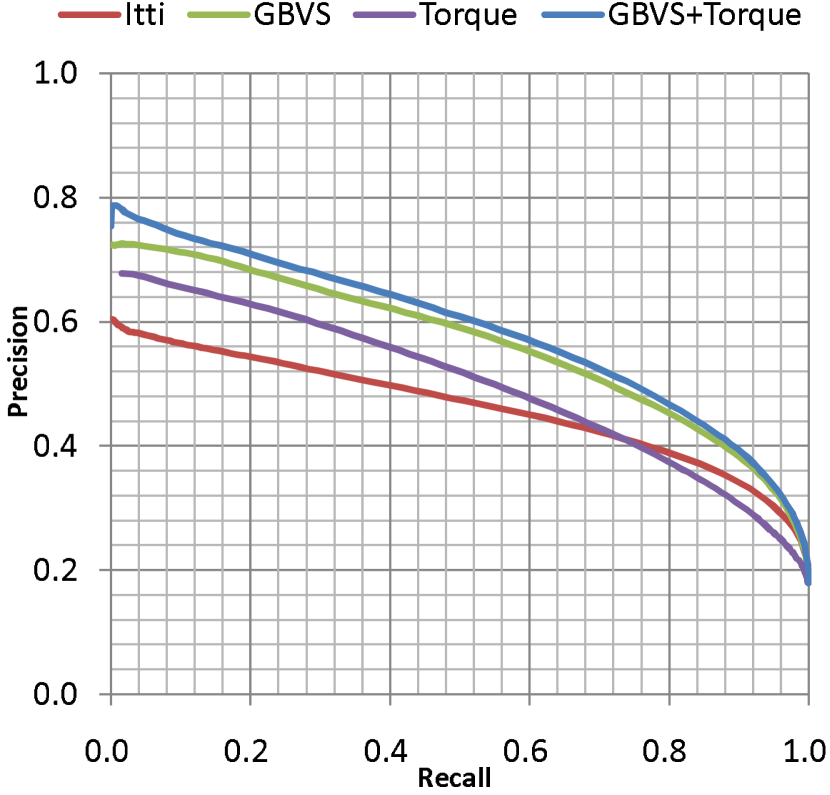
As discussed in section 3.2.3 the torque operator tends to produce extrema at points surrounded by boundary edges, and for patch sizes corresponding to object size. This property of the torque operator is expected to be useful as a cue for bottom-up visual attention. In the following experiment, we computed two torque-based saliency maps. One is generated as mixture of Gaussians with the Gaussian distributions centered at the extrema in the torque volume, and the other is a weighted sum of the generated saliency map and the graph-based visual saliency (GBVS) by Harel et al. [28]. We used weights of 0.3 for the torque-based saliency map and 0.7 for the GBVS, which were found empirically from evaluations on subsets of the dataset.

We used the eye tracking data by Judd et al. [34] to generate ground truth saliency maps. Fixation points were extracted from the data, and saliency maps were generated as mixture of Gaussian distributions centered at the fixation points, and the generated saliency maps were normalized in the range $[0,1]$. The ground truth saliency maps were binarized by a threshold (we used 0.5) in the quantitative comparison.

We resized the test images such that the shorter side of the images was 150 pixels, in order to reduce computational time and standardize the image size. The standard deviation of the Gaussian distributions used to generate the ground truth and torque-based saliency maps were both set to 25 pixels.

The torque-based saliency maps were quantitatively compared with the saliency maps of [32] and [28]. We binarized the computed saliency maps for a set of threshold values equally distant in $[0,1]$, and evaluated precision and recall of the binarized saliency maps as follows:

$$P=\frac{TP}{TP+FP},\quad R=\frac{TP}{TP+FN},\quad$$ (19)

$$TP=\left|S\cap\mathcal{G}\right|,FP=\left|S\cap\overline{\mathcal{G}}\right|,FN=\left|\overline{S}\cap\mathcal{G}\right|,$$ (20)

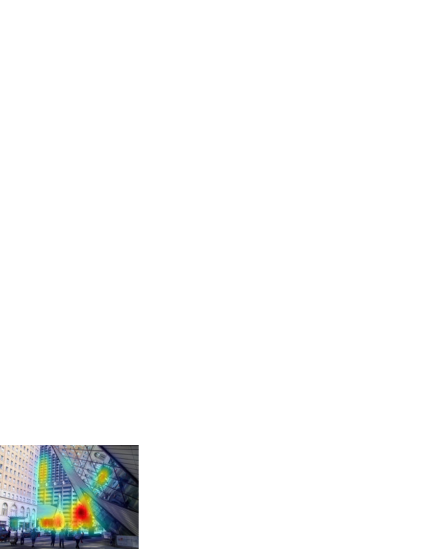
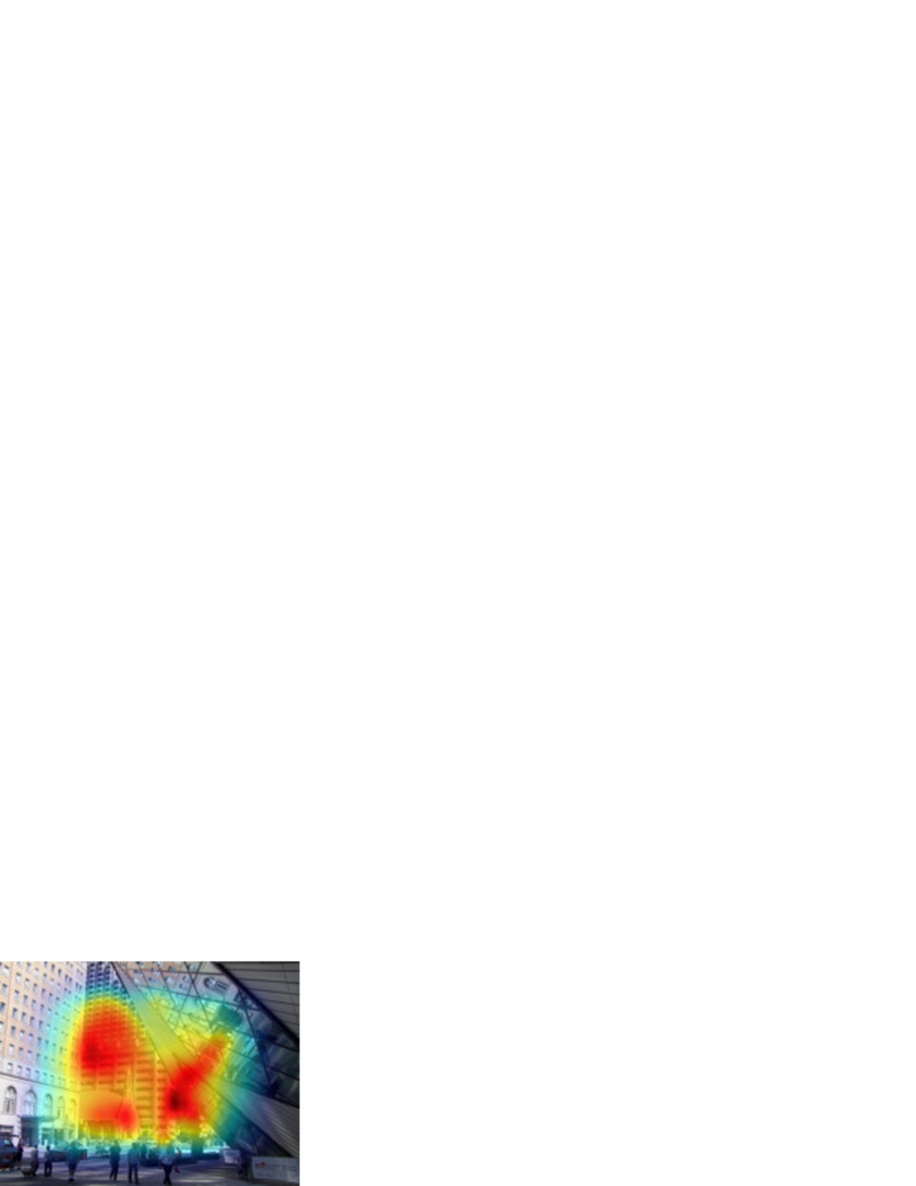
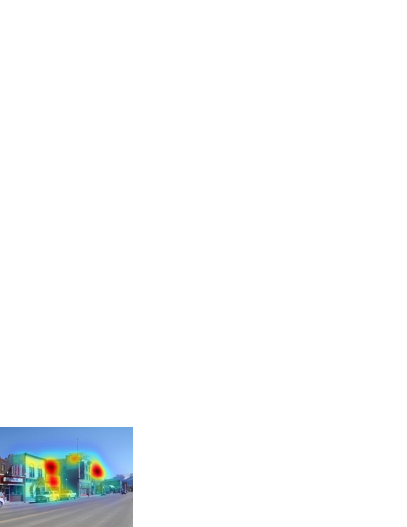
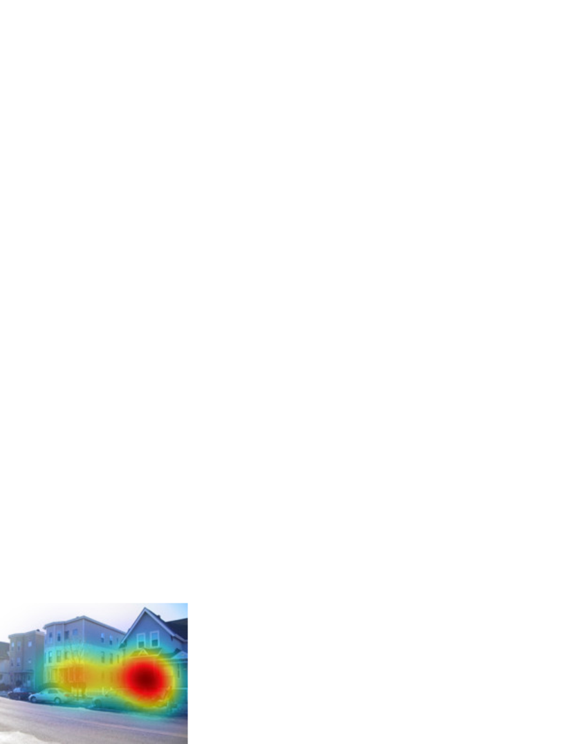
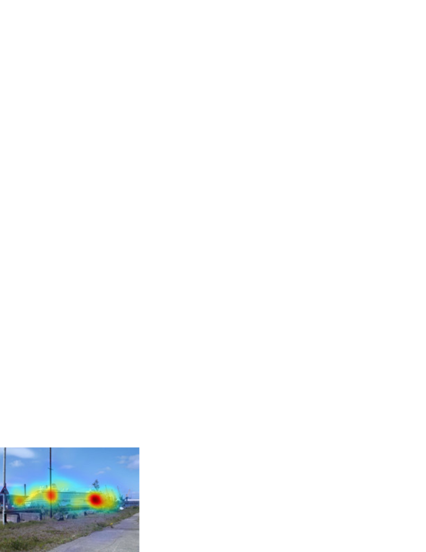
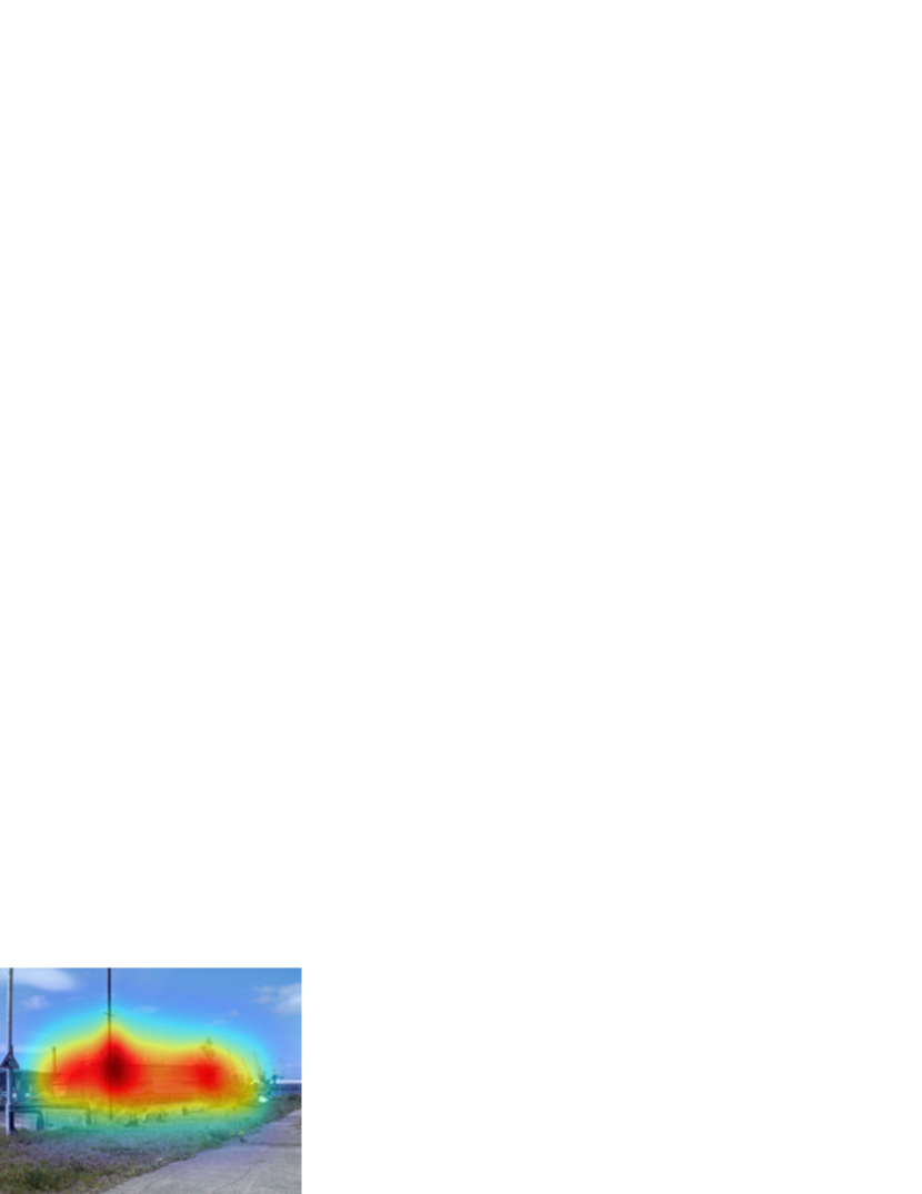
where $S$ is the binarized saliency map, and $\mathcal{G}$ is the binarized ground truth saliency map. $P$ and $R$ denote precision and recall respectively. $TP$, $FP$, $FN$ are true positive, false positive, and false negative, respectively. Fig. 12 shows the ROC curves and maximum F-measures computed from the 898 test images in the dataset. Examples of computed saliency maps along with the ground-truth are shown in Fig. 13. The quantitative comparison shows that the attention map based only on torque does not outperform GBVS. However, the torque measure as additional mid-level visual cue improves the quality of GBVS.

	method F-measure Itti 0.528 GBVS 0.588 Torque 0.538 GBVS+Torque 0.599
(a)	(b)

Figure 12: Evaluation of attention models. (a) ROC curves. (b) F-measure scores.

Itti et al.	GBVS	Troque	GBVS+Torque	Ground truth
0.608	0.486	0.687	0.544
0.700	0.718	0.789	0.794
0.558	0.604	0.481	0.585
0.775	0.795	0.774	0.811
0.690	0.760	0.815	0.818

Figure 13: Examples of Visual Attention. Saliency maps computed by four different methods and the ground-truth saliency map are overlayed on the respective test images. The maximum F-measure is shown below each saliency map.

4.2 Boundary Detection

In our boundary detection we use the torque volume to reweigh edges according to their contribution to large torque values. The contribution of an edge point to torque values of different patches can be obtained as:

$$\upsilon_{q}=\sum_{\left\{P|q\in P\right\}}\tau_{p\left(P\right)q},$$ (21)

where $p\left(P\right)$ indicates the center of the patch $P$, and $q$ is an edge point. The idea is the same as for the attention mechanism. Extrema in the torque volume indicate the existence of edges surrounding the center of a patch. Therefore, edges on object boundaries should have a large contribution to extrema (eq. 21). Edges are strengthened by combining the original edge with the value of this contribution as follows:

$$d_{s}=\frac{1}{1+e^{-\left(c_{0}+c_{1}d_{o}+c_{2}d_{\tau}\right)}},$$ (22)

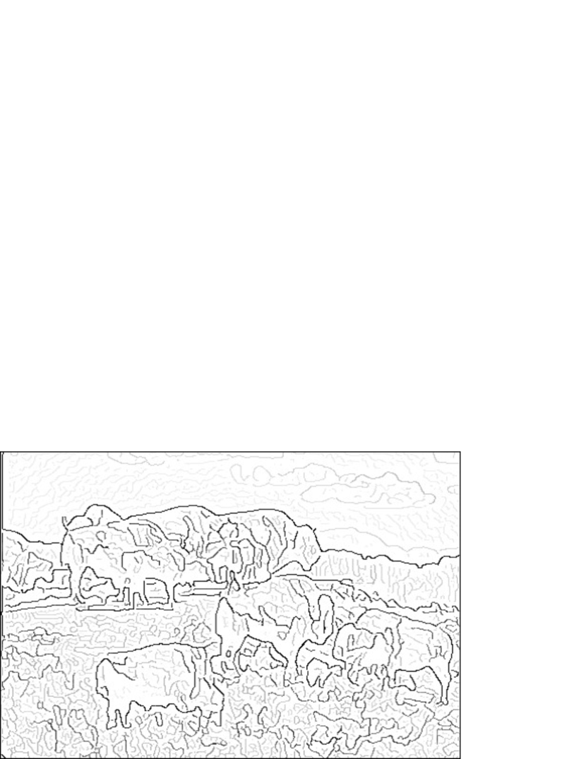
where $d_{o}$ is the original edge intensity, and $d_{\tau}$ is the normalized torque contribution. The computed edge’s contribution to torque is normalized into $[0,1]$. $c_{0}$, $c_{1}$, and $c_{2}$ are constants. We call the edges reweighted by the value $d_{s}$ in eq. (22) Strengthened edges. Examples of such strengthened edges are shown in Fig. 14. In this experiment, the constant parameters $c_{0}$, $c_{1}$ and $c_{2}$ were set to -2.54, 1.86 and 2.69, respectively, and these parameter were learned using training images. Canny edges were used to compute the torque as shown in (b). As can be seen from (c), the strengthened edges tend to be stronger at boundary edges of objects, while weaker at texture edges.

We used the Berkeley dataset [51] to quantitatively evaluate the improvement of boundary detection. While the Canny edge method scored 0.57, the torque-based strengthened edge method using the Canny edges increased the score to 0.59 in the F-measure of the Berkeley benchmark.

(a)	(b)	(c)

Figure 14: Examples of Strengthened edges. (a) Test images. (b) Canny edges. (c) Strengthened edges. The Canny edges shown in (b) are used to compute the Strengthened edges in (c).

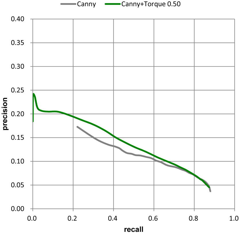
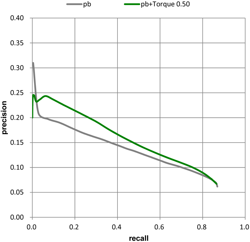
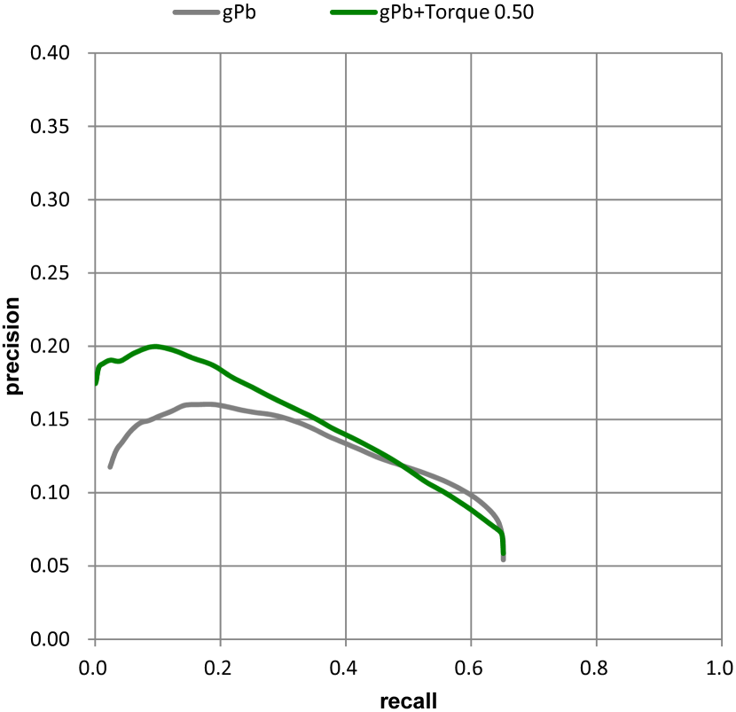
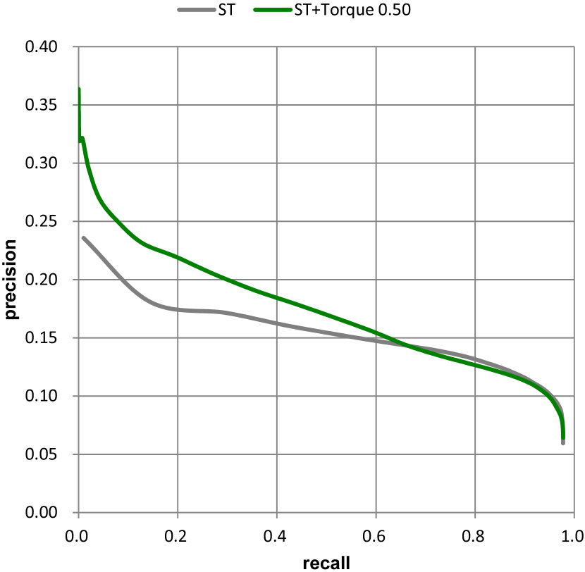
In a second experiment we evaluated the torque on a dataset that is focused on objects. We used the images and boundary annotations for the car side category in the Caltech dataset [22]. Edge maps were computed using Canny, pb boundary [51], and gPb boundary detection [4], and these edge maps were used to derive the torque. Then the torque-based strengthened edges were computed and combined with the base edge maps. Here we simply used a weighted sum to combine the two terms as follows:

$$d_{s}=(1-\alpha)d_{o}+\alpha d_{\tau},$$ (23)

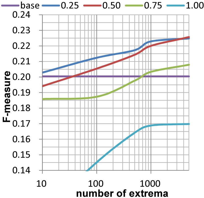
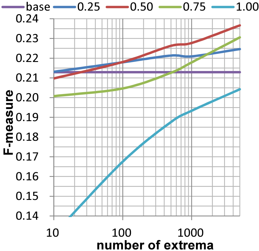
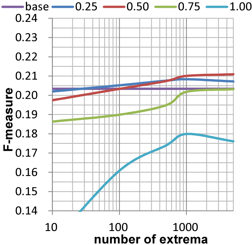
where $d_{o}$ denotes the edge map, $d_{\tau}$ the torque contribution map, and $d_{s}$ the strengthened edge map. We computed Precision and Recall for the strengthened edge maps $d_{s}$ and the base edge maps $d_{o}$, and evaluated the maximum F-measure as a function of parameter $\alpha$ and the number of torque extrema in the computation of the torque contribution map, as shown in Fig 15. Based on this evaluation, $\alpha$ was set to 0.5. In addition, we evaluated the recently proposed method of Sketch Tokens [44] for boundary detection and the effect of edge strengthening on this method. The precision-recall (PR) curve for all four methods are shown in Fig 16. Comparing in Fig. 15 the maximum F-measure of the strengthened edge maps with the base edge maps, we can verify that the torque operator improves silhouette boundary detection. Table 1 summarizes the results for $\alpha=0.5$ and 5000 torque extrema for all four methods.

Method	F-measure
Canny	0.20
Torque (Canny)	0.23
pb	0.21
Torque (pb)	0.24
gPb	0.20
Torque (gPb)	0.21
Sketch Tokens	0.24
Torque (Sketch Tokens)	0.25

Table 1: F-measure comparison in boundary detection between base edge maps and torque-based strengthened edge maps.

(a) Canny	(b) pb	(c) gPb

Figure 15: Performance of boundary detection evaluated by the maximum F-measure as a function of $\alpha$ and the number of extrema. Three edge detection methods were used to compute base edge maps: (a) Canny edges, (b) pb edges, and (c) gPb edges. The base edge maps were blended with the torque contribution map to generate strengthened edge maps. In the legend base refers to the base edge maps, and the numbers indicate the weight $\alpha$ in eq.(23) used to obtain strengthened edge maps.

Figure 16: Precision-recall (PR) curves for boundary detection. The torque-based strengthened edge map (green ) is is compared to the base edge map (gray) for: (a) Canny edges, (b) pb edges, (c) gPb edges, and (d) Sketch tokens edges.

(a) Canny	(b) pb
(c) gPb	(d) Sketch Tokens

4.3 Segmentation

Next the torque operator is demonstrated for segmentation in two graphcut approaches, and a quantitative comparison to other methods is given. The first approach is a generic multi-region segmentation, and the second is a figure-ground segmentation. Both approaches basically rely on the torque as attention and scale selection mechanism. The attended region is then utilized to obtain foreground color models or to strengthen edges.

4.3.1 Multi-region Segmentation

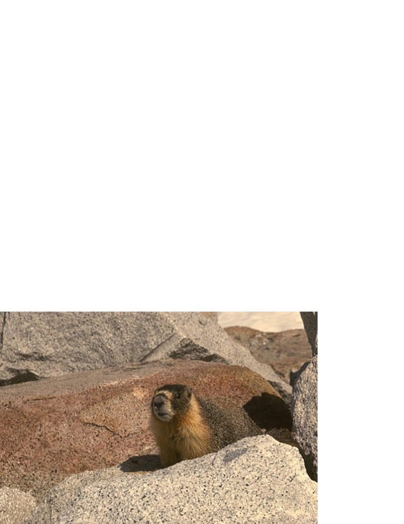
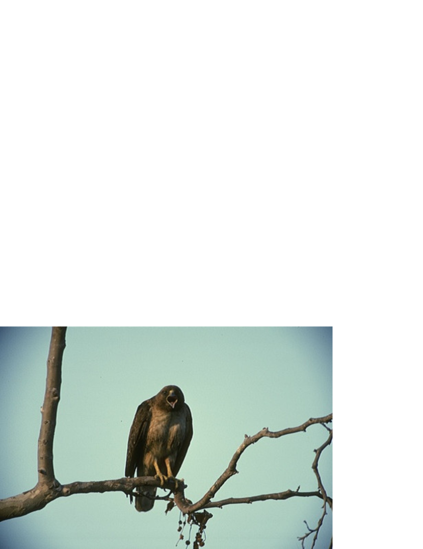
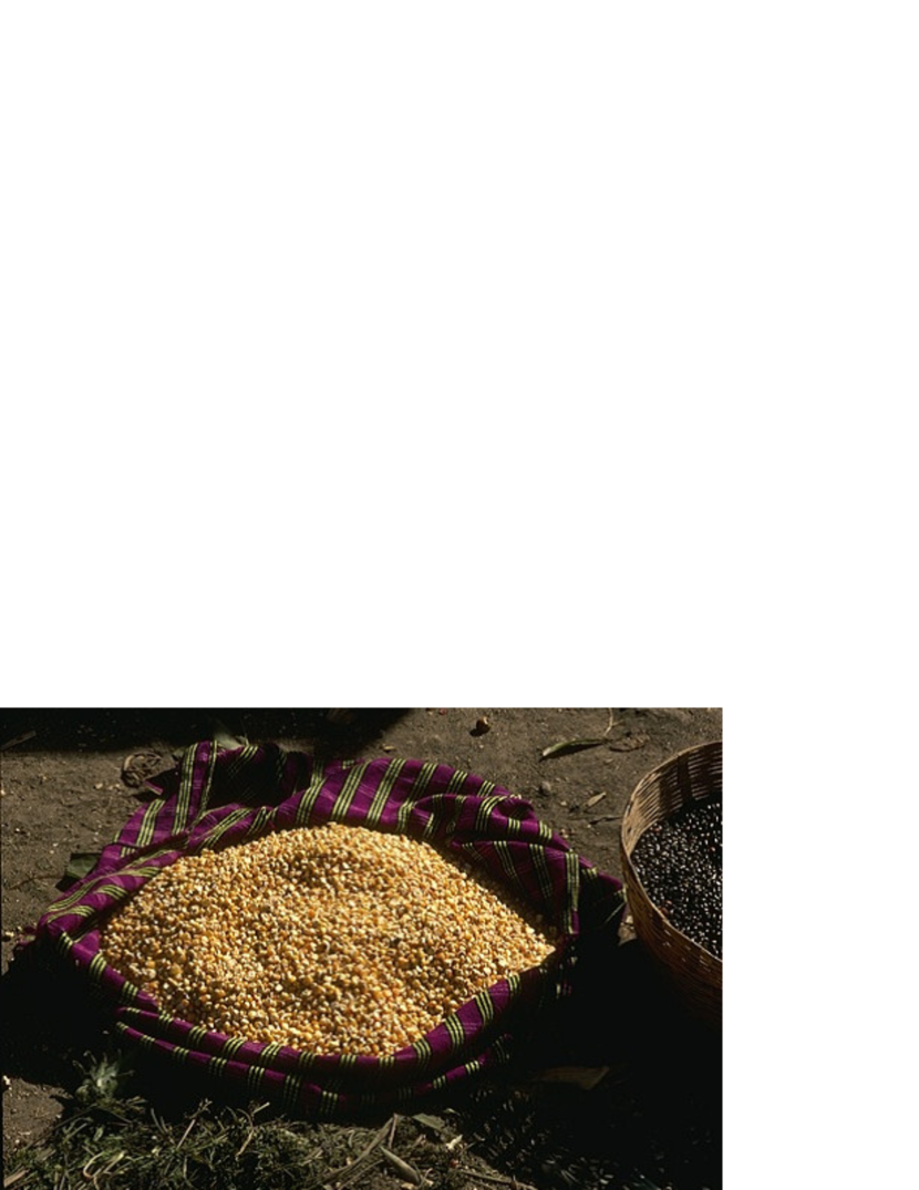
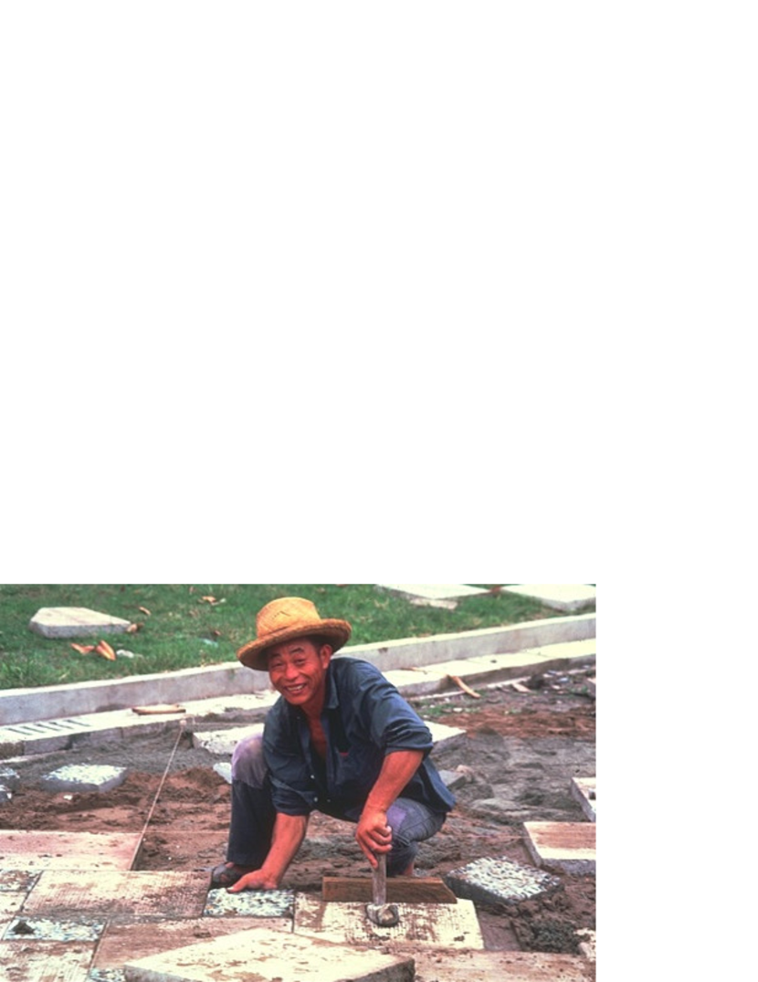
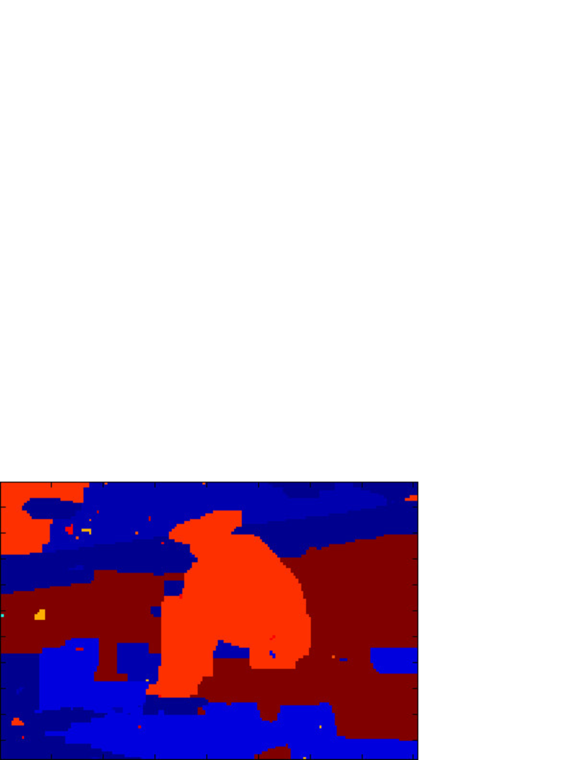
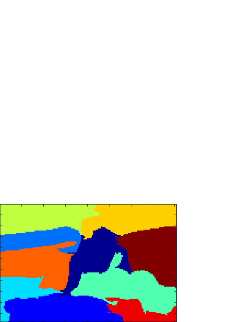
We used the torque extrema and their corresponding scales to obtain image regions likely to correspond to interesting elements of the image. In this experiment, each such image region is modeled by a color histogram, and these histograms are used to create the weights in a multi-label graph-cut segmentation. The data term in the graph-cut is derived from how well the color at a pixel matches each color model, and the smoothness term is based on color similarity of adjacent pixels. The segmentation method was applied to the Berkeley image data set and the quality of the segmentation was evaluated using the covering criteria [3]. We compared against the normalized cut segmentation [69]. Fig. 17 shows example segmentations of the two segmentation methods. A visual evaluation shows, that the graphcut method better segments than the normalized cut, in the sense of being able to better extract object-like regions, and the quantitative evaluation demonstrates that the graphcut method clearly outperforms the normalized cut (Table 2).

(a)	(b)	(c)

Figure 17: Examples of generic multi-region segmentation: (a) Test images. (b) Segmentation using the torque operator (c) Segmentation using the normalized cut.

Table 2: Comparison of multi-region segmentations based on the covering criteria.

Method	Covering
Torque	0.429
N-Cut	0.390

4.3.2 Figure-ground Segmentation

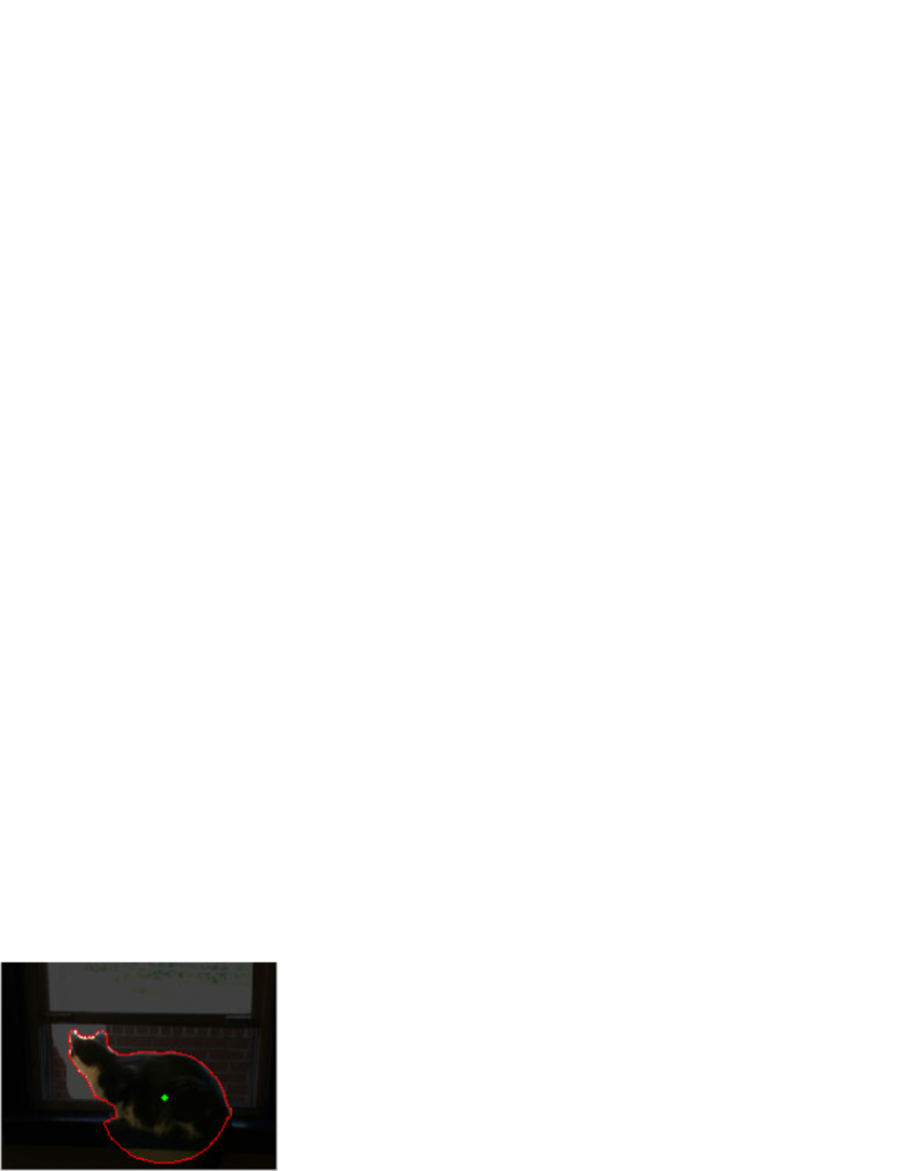
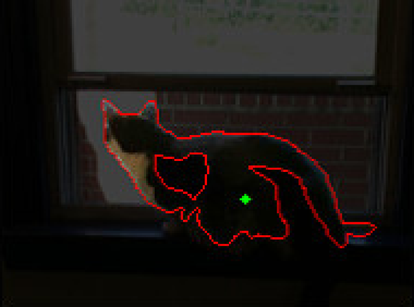
The strengthened edges are expected to be useful for figure-ground segmentation because object boundaries are emphasized. Here we demonstrate an edge-based graph cut algorithm using the strengthened edges. For a quantitative evaluation of figure-ground segmentation, we used the dataset by Stein et al. [71], which has ground truth segmentations for multiple foreground objects. For each reference image in the data set we selected a single foreground object, and used the centroid of the object as fixation point. Then we applied the fixation based segmentation algorithm of [54]. This algorithm separates foreground from background using a graphcut on a probability map of edges in a polar coordinate system. Different visual cues were used in the graph-cut segmentation for comparison: the Canny edge map, the boundary probability map (Pb) [52], a strengthened edge map using Canny edges, and a strengthened edge map using Pb edges. So we can separate the effect of the torque measure, we used as strengthened edge directly the normalized torque value contribution, $d_{\tau}$. The quality of segmentation was evaluated by the segmentation covering [3]. In the case of foreground-background segmentation this measure amounts to the ratio of the true positive area and the union of computed segmentation and ground truth segmentation.

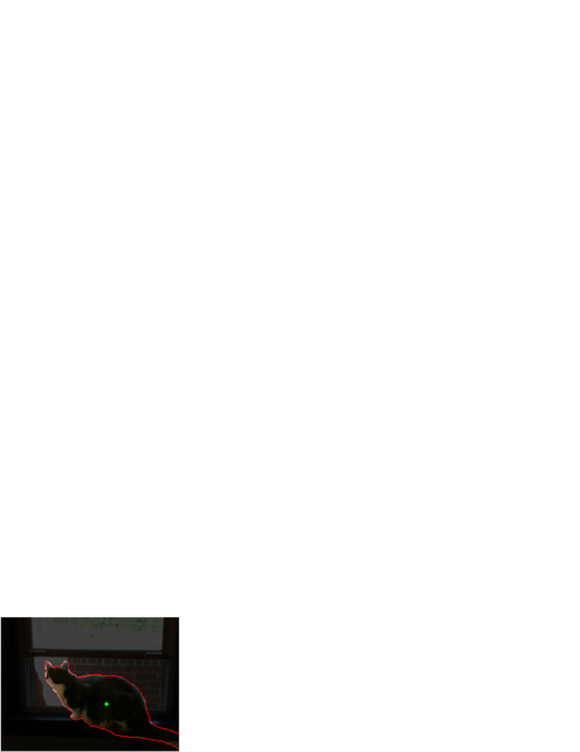
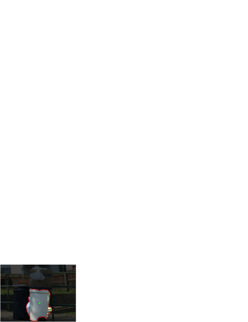
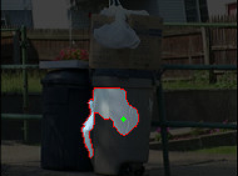
Table 3 shows the results of the comparison for the dataset. For each visual cue the average covering over 28 test images is shown. As can seen from the table, adding the torque significantly improves the segmentation. Finally, we also compared with the non-edge based level-set segmentation by Chan and Vese [11]. From the the performance of this method, we can see that the segmentation of objects for this data set, given only the fixation point, is a challenging task. Examples of segmentation results are shown in Fig. 18.

Table 3: Comparison of foreground-background segmentations based on the covering criteria. The notation Torque (Canny) and Torque (pb) refer to strengthened edges by the torque operator using as base Canny or the pb edges, respectively.

Visual Cue	Covering
Canny	0.32
Torque (Canny)	0.47
pb	0.40
Torque (pb)	0.48
Chan-Vese	0.21

(a)	(b)	(c)	(d)

Figure 18: Example of a segmentation: (a) using Canny edges (b) using strengthened edges by the torque (c) using the Chan-Vese method [11]. (d) Ground truth. The green dot denotes the fixation point.

4.4 Recognition

This section summarizes experiments from [84], where we used the torque mechanism for object recognition in the bag-of-features framework. The approach consists of two steps: a patch detection, and a patch description. First, torque value extrema in space and scale and their corresponding patches are detected. These patches are separated into minima, i.e the dark patches on brighter background and maxima, i.e. bright patches on darker background. This detection scheme is called Maximal/Minimal Torque Patch (MTP) detector.

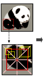
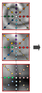
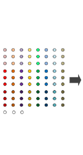
Second, the density and variance of the local edge structure is described in a multi-scale manner in the so-called Multiscale Torque (MST) descriptor. For a given patch regions of multiple sizes having an overlap with the patch along the eight axes at discrete space intervals are selected and their torque values are concatenated into a vector. To keep the number of selected areas the same for all patches, the step size is adapted to the patch size, and to make it robust to rotation, the patch is rotated such that its x-axis becomes the direction closest in direction to the vector pointing from the patch center to the centroid of the edges inside the patch P (see Fig. 19).

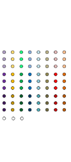(a) An MTP patch	(b) Torque magnitudes	(c) Multi-scale sampling	(d) Orientation alignment

Figure 19: Outline of MST descriptor. From left to right: (a) An interesting patch is detected by the MTP detector. (b) The torque magnitudes of regions centered at points inside the detected patch are computed. (c) The torque values are sampled along 8 directions at several scales. The sampled values are collected and concatenated as the local feature of the MTP patch. (d) Alignment of the orientation of the feature by circular-shifting.

This descriptor was evaluated for object recognition following the bag of features (BoF) representation paradigm evaluated on the Caltech-101 dataset. Table 4 shows the performance of the method in comparison to a number of top feature-based recognition methods (which were also used for comparison in [81]). As can be seen, by itself the torque-based method performs about the same as [33], but does not perform as well as methods based on SIFT-based features (such as [8], [85], and [81]). This is because, these images are better captured by texture content (extracted through SIFT features). However by combining the contour-based feature with SIFT, better performance was achieved. Our implementation of the SIFT feature followed that of [81], and we combined the two features by concatenating them into a single vector and weighing them 1:2 (ours v.s. SIFT). Our method had an additional $2.45\%-4.66\%$ accuracy gain over the best results of other methods with respect to different sizes of the training set. These results demonstrate that the proposed contour-based feature does capture meaningful information of object contour and adds to objection recognition.

	5	10	15	20	25	30
Jain et al. [33]	-	-	61.00	-	-	69.10
Boiman et al. [8]	-	-	65.00	-	-	70.40
Yang et al. [85]	-	-	67.00	-	-	73.20
Wang et al. [81]	51.15	59.77	65.43	67.74	70.16	73.44
Ours	48.17	57.65	62.33	65.32	67.39	68.97
Ours + SIFT	53.60	64.01	69.15	72.40	74.52	76.22

Table 4: Classification accuracy for different methods on the Caltech-101 dataset.

5 Conclusion

We introduced a new tool of mid-level vision, the Torque Operator, and explored its fundamental properties using both theory and experiments. The torque operator creates maps, which encode the structure of edges within patches, and it tends to generate larger absolute values when edges are aligned in a way surrounding the center of the patch, and the region enclosed by these edges matches the size of patch. This basic property was first discussed and examined on synthesized images. Then, this property was demonstrated in the applications of attention, boundary detection, segmentation, and object recognition. Experiments showed that for all these applications the torque operator enhances the performance. An efficient implementation of the torque based on integral images has also been provided (see [76]).

6 Extension and Outlook

We believe that the concept of a grouping mechanism implemented via image processing operations is a powerful concept, and there are many way this concept can be generalized.

This paper discussed a number of ways on how to use the Torque operator in bottom-up processing for various applications. An immediate extension would be to use the information it provides in different ways. For example the torque value itself is also expected to be a useful visual cue for segmentation. Furthermore, the torque operator could be applied to image gradient maps instead of edge maps. Such a torque measure can be derived as the average brightness difference between the inside and the boundary of an image patch (see Appendix A).

The general concept of a mid-level operator acting as grouping mechanism can be developed along a number of directions. We could have various mechanisms tuned to different edge configurations. For example, instead of adding curve contribution, such that circles are favored, we can add them such that radial lines or spirals are favored, and this way create a set of operators tuned to semi-global patterns. We demonstrated such operators for boundary ownership classification [73], but this generalization could be useful also for texture or object recognition.

While in this paper we applied the torque to edges of single images, the torque operator is applicable also to geometric edges, such as depth edges and motion edges. Because these edges are due to depth discontinuities, which usually are at the boundary of surfaces, it is expected that such a torque operator will perform better for finding objects.

It is clear that pure bottom-up processing has its limitations, and object recognition or object segmentation in single images requires higher level knowledge. The torque mechanism as a mid-level grouping tool can be modified also to interact with higher-level processes encoding semantic information. We believe that there is room for research that embeds mid-level operators into object recognition and learning. Such an approach was demonstrated in [75] and [74], where torque-like operators were tuned to specific shapes. Contour processing of specific object classes using generalized torque then proceeds in two steps. First the bottom-up torque acts as an attention (or saliency) mechanism. Then torque-like operators, that are tuned to respond to learned categories of objects, object parts, or attributes can be used in task-guided top-down processing.

7 Acknowledgements

The support of the European Union under the Cognitive Systems program (project POETICON++), the National Science Foundation under INSPIRE grant SMA 1248056, and DARPA through U.S. Army grant W911NF-14-1-0384 are gratefully acknowledged.
The authors would like to thank Daniel Dementhon for sharing his code, which originated this project.

Appendix A Torque based on Gradient

In previous sections, the torque was defined on edges, where edges were normalized as unit vectors. Next we consider a slightly different formulation of the torque, which considers the strength of edges. Images have strong edges and weak edges, and the strength is defined by the gradient. As will be shown next, a torque of patches defined on gradients can be computed simply from the intensity in the area and at the boundary of the patch.

The gradient torque is defined as follows:

$$\tau_{pq}=\vec{r}_{pq}\times\tilde{\nabla}I\left(q\right),$$ (24)

where $p$ is the center point and $q$ is some point on the image. $\vec{r}_{pq}$ is the displacement vector from $p$ to $q$. $\tilde{\nabla}I\left(q\right)$ is the image gradient at $q$ rotated by 90 degree, i.e. $\left(\frac{\partial I}{\partial y},-\frac{\partial I}{\partial x}\right)$, representing an edge-like vector. Similarly, the gradient torque for a patch is defined as:

$$\tau_{P,p}=\frac{1}{2\left|P\right|}\int_{q\in P}\tau_{pq}dq,$$ (25)

where $P$ is the patch, and the integral is taken over the patch.

Next we show that the gradient torque of a patch can be computed as the difference of the average image intensity inside the patch and the average image intensity on the patch boundary. Considering a disk patch, it thus amounts to:

$$\tau_{P,p} =\frac{1}{\pi R^{2}}\int^{R}_{0}\int^{\pi}_{-\pi}I\left(r,\theta\right)\cdot rd\theta dr$$

$$-\frac{1}{2\pi R}\int^{\pi}_{-\pi}I\left(R,\theta\right)\cdot Rd\theta,$$ (26)

where $I\left(r,\theta\right)$ is the image intensity at $\left(r,\theta\right)$ in the polar coordinate system. Without loss of generality, it is assumed that the center of the patch is the origin of the coordinate system so that $\vec{r}_{pq}=\left(x,y\right)$ for $q=\left(x,y\right)$. Then, using the substitution $\left(x,y\right)=\left(r\cos\theta,r\sin\theta\right)$, eq.(26) can be deduced as follows:

$$\tau_{P,p} =\frac{1}{2\pi R^{2}}\int^{R}_{0}\int^{\pi}_{-\pi}\left\{x\left(-\frac{\partial I}{\partial x}\right)-y\frac{\partial I}{\partial y}\right\}rd\theta dr$$ (27)

$$=\frac{1}{2\pi R^{2}}\int^{R}_{0}\int^{\pi}_{-\pi}\cos\theta\left(\sin\theta\frac{\partial I}{\partial\theta}-r\cos\theta\frac{\partial I}{\partial r}\right)$$ (28)

$$-\sin\theta\left(\cos\theta\frac{\partial I}{\partial\theta}+r\sin\theta\frac{\partial I}{\partial r}\right)rd\theta dr$$

$$=-\frac{1}{2\pi R^{2}}\int^{R}_{0}\int^{\pi}_{\pi}r^{2}\frac{\partial I}{\partial r}d\theta dr$$ (29)

$$=-\frac{1}{2\pi R^{2}}\int^{\pi}_{-\pi}\left\{R^{2}I\left(R,\theta\right)-\int^{R}_{0}2rI\left(r,\theta\right)dr\right\}d\theta.$$ (30)

Eq. (30) is equivalent to eq. (26), which concludes the proof.

References

- [1] B. Alexe, T. Deselaers, and V. Ferrari. Measuring the objectness of image windows. IEEE Transactions on Pattern Analysis and Machine Intelligence, 34(11):2189–2202, 2012.
- [2] Sharon Alpert, Meirav Galun, Ronen Basri, and Achi Brandt. Image segmentation by probabilistic bottom-up aggregation and cue integration. In Conference on Computer Vision and Pattern Recognition, 2007.
- [3] P. Arbeláez, M. Maire, C. Fowlkes, and J. Malik. From contours to regions: An empirical evaluation. In Conference on Computer Vision and Pattern Recognition, 2009.
- [4] P. Arbeláez, M. Maire, C. Fowlkes, and J. Malik. Contour detection and hierarchical image segmentation. IEEE Transactions on Pattern Analysis and Machine Intelligence, 33(5):898–916, 2011.
- [5] Serge Belongie, Jitendra Malik, and Jan Puzicha. Shape matching and object recognition using shape contexts. IEEE Transactions on Pattern Analysis and Machine Intelligence, 24(4):509–522, 2002.
- [6] K. Bitsakos, C. Fermüller, and Y. Aloimonos. An experimental study of color-based segmentation algorithms based on the mean-shift concept. In Nikos Paragios Kostas Daniilidis, Petros Maragos, editor, Proc. European Conference on Computer Vision, volume 6312 2010 of Lecture Notes in Computer Science, 2010.
- [7] Andrew Blake and Michael Isard. Active Contours. Springer, 2000.
- [8] O. Boiman, E. Shechtman, and M. Irani. In defense of nearest-neighbor based image classification. In Conference on Computer Vision and Pattern Recognition, 2008.
- [9] Yuri Boykov and Vladimir Kolmogorov. An experimental comparison of min-cut/max-flow algorithms for energy minimization in vision. IEEE Transactions on Pattern Analysis and Machine Intelligence, 26(9):1124–1137, 2004.
- [10] Yuri Boykov, Olga Veksler, and Vladimir Kolmogorov. Fast approximate energy minimization via graph cuts. IEEE Transactions on Pattern Analysis and Machine Intelligence, 23(11):1222–1239, 2001.
- [11] T. F. Chan and L. A. Vese. Active contours without edges. IEEE Transactions on Pattern Analysis and Machine Intelligence, 10(2):266–277, 2001.
- [12] M.M. Cheng, Z. Zhang, W.Y. Lin, and P. Torr. Bing: Binarized normed gradients for objectness estimation at 300fps. In Proc. IEEE Conference on Computer Vision and Pattern Recognition, pages 3286–3293, 2014.
- [13] Dorin Comaniciu and Peter Meer. Mean shift: A robust approach toward feature space analysis. Journal of Neurophysiology, 97:4310–4326, 2007.
- [14] Edward Craft, Hartmut Schütze, Ernst Niebur, and Rüdiger von der Heydt. A neural model of figure-ground organization. J. Neurophysiol., 97(6):4310–4326, 2007.
- [15] A. Criminisi, G. Cross, A. Blake, and V. Kolmogorov. Bilayer segmentation of live video. In Conference on Computer Vision and Pattern Recognition, 2006.
- [16] Navneet Dalal and Bill Triggs. Histograms of oriented gradients for human detection. In Cordelia Schmid, Stefano Soatto, and Carlo Tomasi, editors, International Conference on Computer Vision & Pattern Recognition, volume 2, pages 886–893, INRIA Rhône-Alpes, ZIRST-655, av. de l’Europe, Montbonnot-38334, June 2005.
- [17] Piotr Dollár, Zhuowen Tu, and Serge Belongie. Supervised learning of edges and object boundaries. In Conference on Computer Vision and Pattern Recognition, 2006.
- [18] Piotr Dollár and C. Lawrence Zitnick. Structured forests for fast edge detection. In International Conference on Computer Vision, pages 1841–1848, 2013.
- [19] W. Einhäuser, M. Spain, and P. Perona. Objects predict fixations better than early saliency. Journal of Vision, 8(14):1–26, 2008.
- [20] Wolfgang Einhäuser, Wolfgang Kruse, Klaus-Peter Hoffmann, and Peter König. Differences of monkey and human overt attention under natural conditions. Vision Research, 46(8-9):1194–1209, 2006.
- [21] J. H. Elder and S. W. Zucker. Computing contour closure. In Proc. European Conference on Computer Vision, 1996.
- [22] Li Fei-Fei, Rob Fergus, and Pietro Perona. One-shot learning of object categories. IEEE Transactions on Pattern Analysis and Machine Intelligence, 28(4):594–611, 2006.
- [23] C. Fermüller, Y. Brodsky, and Y. Aloimonos. Motion segmentation: a synergistic approach. In Proc. IEEE Conference on Computer Vision and Pattern Recognition, volume 2, 1999.
- [24] Vittorio Ferrari, Tinne Tuytelaars, and Luc Van Gool. Object detection by contour segment networks. In Proceeding of the European Conference on Computer Vision, volume 3953 of LNCS, pages 14–28. Elsevier, June 2006.
- [25] Meirav Galun, Ronen Basri, and Achi Brandt. Multiscale edge detection and fiber enhancement using differences of oriented means. In International Conference on Computer Vision, pages 1–8, 2007.
- [26] Michael Grabner, Helmut Grabner, and Horst Bischof. Fast approximated sift. In Asian Conference on Computer Vision, pages 918–927, 2006.
- [27] Gideon Guy and Gerard Medioni. Inferring global perceptual contours from local features. In IEEE Conference on Computer Vsion and Pattern Recognition, pages 786–787, 1993.
- [28] Jonathan Harel, Christof Koch, and Pietro Perona. Graph-based visual saliency. In Conference on Neural Information Processing Systems, pages 545–552, 2006.
- [29] A. Hollingworth, C.C. Williams, and J.M. Henderson. To see and remember: Visually specific information is retained in memory from previously attended objects in naturalscenes. Psychonomic Bulletin and Review, 8:761–768, 2001.
- [30] L. Holm, J. Eriksson, and L. Andersson. Looking as if you know: Systematic object inspection precedes object recognition. Journal of Vision, 8(4):1–7, 2008.
- [31] Jan Hosang, Rodrigo Benenson, Piotr Dollár, and Bernt Schiele. What makes for effective detection proposals? IEEE Transactions on Pattern Analysis and Machine Intelligence, page accepted for publication, 2016.
- [32] L. Itti, C. Koch, and E. Niebur. A model of saliency-based visual attention for rapid scene analysis. IEEE Transactions on Pattern Analysis and Machine Intelligence, 20(11):1254–1259, 1998.
- [33] P. Jain, B. Kullis, and K. Grauman. Fast image search for learned metrics. In Conference on Computer Vision and Pattern Recognition, 2008.
- [34] T. Judd, K. Ehinger, F. Durand, and A. Torralba. Learning to predict where humans look. In IEEE International Conference on Computer Vision, 2009.
- [35] F. Jurie and C. Schmid. Scale-invariant shape features for recognition of object categories. In Conference on Computer Vision and Pattern Recognition, 2004.
- [36] Ryan Kennedy, Jean Gallier, and Jianbo Shi. Contour cut: identifying salient contours in images by solving a hermitian eigenvalue problem. In Conference on Computer Vision and Pattern Recognition, pages 2065–2072, 2011.
- [37] Pushmeet Kohli, L’Ubor Ladický, and Philip H. Torr. Robust higher order potentials for enforcing label consistency. International Journal of Computer Vision, 82(3):302–324, 2009.
- [38] Iasonas Kokkinos. Highly accurate boundary detection and grouping. In IEEE Conf. on Computer Vision and Pattern Recognition (CVPR), 2010.
- [39] Iasonas Kokkinos, Petros Maragos, and Alan Yuille. Bottom-up and top-down object detection using primal sketch features and graphical models. In IEEE Conf. on Computer Vision and Pattern Recognition (CVPR), 2006.
- [40] V. Kolmogorov, A. Criminisi, A. Blake, G. Cross, and C. Rother. Bilayer segmentation of binocular stereo video. In Conference on Computer Vision and Pattern Recognition, 2005.
- [41] Peter Kontschieder, Samuel Rota Bulo, Horst Bischof, and Marcello Pelillo. Structured class-labels in random forests for semantic image labelling. In IEEE Int. Conference on Computer Vision, pages 2190–2197, 2011.
- [42] M. P. Kumar, P. H. S. Torr, and A. Zisserman. Extending pictorial structures for object recognition. In British Machine Vision Conference, 2004.
- [43] Bastian Leibe, Ales Leonardis, and Bernt Schiele. Combined object categorization and segmentation with an implicit shape model. In Workshop on Statistical Learning in Computer Vision, ECCV, 2004.
- [44] Joseph J. Lim, C. Lawrence Zitnick, and Piotr Dollar. Sketch tokens: A learned mid-level representation for contour and object detection. In Conference on Computer Vision and Pattern Recognition, 2013.
- [45] T. Lindeberg. Scale-Space Theory in Computer Vision. Kluwer, Boston, 1994.
- [46] Tony Lindeberg. Detecting salient blob-like image structures and their scales with a scale-space primal sketch: a method for focus-of-attention. International Journal of Computer Vision, 11(3):283–318, 1998.
- [47] Tony Lindeberg. Feature detection with automatic scale selection. International Journal of Computer Vision, 30:79–116, 1998.
- [48] David G. Lowe. Distinctive image features from scale-invariant keypoints. Int. J. Comput. Vision, 60(2):91–110, November 2004.
- [49] Julien Mairal, Francis Bach, Jean Ponce, Guillermo Sapiro, , and Andrew Zisserman. Video object segmentation using stereo-derived depth matps. In 27th Workshop of the AAPR/ÖAGM, pages 197–204, 2003.
- [50] David Marr. Vision A Computational Investigation into the Human Representation and Processing of Visual Information. MIT Press, 1982.
- [51] D. Martin, C. Fowlkes, D. Tal, and J. Malik. A database of human segmented natural images and its application to evaluating segmentation algorithms and measuring ecological statistics. In International Journal of Computer Vision, volume 2, pages 416–423, 2001.
- [52] D. R. Martin, C. C. Fowlkes, and J. Malik. Learning to detect natural image boundaries using local brightness, color, and texture cues. IEEE Transactions on Pattern Analysis and Machine Intelligence, 26(5):530–549, 2004.
- [53] Yansheng Ming, Hongdong Li, and Xuming He. Connected contours: A new contour completion model that respects the closure effect. In IEEE International Conference on Computer Vision, pages 829–836, 2012.
- [54] Ajay K. Mishra, Cornelia Fermüller, and Yiannis Aloimonos. Active segmentation for robots. In IROS, 2009.
- [55] D. Mumford and J. Shah. Functions and associated variational problems. Communications on Pure and Applied Mathematics, 42(5):577–685, 1989.
- [56] Morimichi Nishigaki, Cornelia Fermüller, and Daniel DeMenthon. The image torque operator: A new tool for mid-level vision. In CVPR’12, pages 502–509, 2012.
- [57] A. S. Ogale, C. Fermüller, and Y. Aloimonos. Detecting independent 3d movement. In E. Bayro-Corrochano, editor, Handbook of Geometric Computing Applications in Pattern Recognition, Computer Vision, Neural computing, and Robotics. Springer Verlag, March 2005.
- [58] A. Opelt, A. Pinz, and A. Zisserman. A boundary-fragment-model for object detection. In European Conference on Computer Vision, 2006.
- [59] S. J. Osher and J. A. Sethian. Fronts propagating with curvature-dependent speed; algorithms based on hamilton-jacobi formulations. Journal of Computational Physics, 79(1):12–49, 1988.
- [60] Saiprasad Ravishankar, Arpit Jain, and Anurag Mittal. Multi-stage contour based detection of deformable objects. In European Conference on Computer Vision, pages 483–496. Springer, 2008.
- [61] X. Ren and J. Malik. A probabilistic multi-scale model for contour completion based on image statistics. In European Conference on Computer Vision, pages 312–327, 2002.
- [62] X. Ren and J. Malik. Learning a classification model for segmentation. In IEEE International Conference on Computer Vision, pages 10–17, 2003.
- [63] Xiaofeng Ren. Multi-scale improves boundary detection in natural images. In European Conference on Computer Vision, 2008.
- [64] Xiaofeng Ren and Liefeng Bo. Discriminatively trained sparse code gradients for contour detection. In F. Pereira, C.J.C. Burges, L. Bottou, and K.Q. Weinberger, editors, Advances in Neural Information Processing Systems 25, pages 584–592. Curran Associates, Inc., 2012.
- [65] Xiaofeng Ren, Charless C. Fowlkes, and Jitendra Malik. Cue integration in figure/ground labeling. In Advances in Neural Information Processing Systems, 2005.
- [66] Hayko Riemenschneider, Michael Donoser, , and Horst Bischof. Using partial edge contour matches for efficient object category localization. In European Conference on Computer Vision, pages 29–42. Springer, 2010.
- [67] C.V. Rother and V. Kolmogorov. Grabcut: Interactive foreground extraction using iterated graph cuts. ACM Transactions on Graphics, 23(3):309–314, 2004.
- [68] T. Schoenemann, S. Masnou, and D. Cremers. The elastic ratio: Introducing curvature into ratio-based image segmentation. IEEE Transactions on Image Processing, 20(9):2565– 2581, 2011.
- [69] Jianbo Shi and Jitendra Malik. Normalized cuts and image segmentation. IEEE Transactions on Pattern Analysis and Machine Intelligence, 22(8):888–905, 2000.
- [70] J. Shotton, A. Blake, and R. Cipolla. Contour-based learning for object detection. In IEEE Int. Conference of Computer Vision, pages I: 503–510, 2005.
- [71] A. N. Stein, T. S. Stepleton, and M. Hebert. Towards unsupervised whole-object segmentation: Combining automated matting with boundary detection. In Conference on Computer Vision and Pattern Recognition, 2008.
- [72] Takahiro Suzuki and Takeshi Ikenaga. Low complexity keypoint extraction based on sift descriptor and its hardware implementation for full-hd 60 fps video. IEICE Trans. on Fundamentals of Electronics, Communications and Computer Science, E96-A(6):1376–1383, 2013.
- [73] Ching L. Teo, Cornelia Fermüller, and Yiannis Aloimonos. Fast 2d border ownership assignment. IEEE Conference on Computer Vision and Pattern Recognition, 2015.
- [74] Ching L. Teo, Cornelia Fermüller, and Yiannis Aloimonos. A gestaltist approach to contour-based object recognition: Combining bottom-up and top-down cues. International Journal of Robotics Research, 34:627–652, 2015.
- [75] Ching L. Teo, Austin Myers, Cornelia Fermüller, and Yiannis Aloimonos. Embedding high-level information into low level vision: Efficient object search in clutter. In IEEE International Conference on Robotics and Automation (ICRA), 2013.
- [76] http://www.umiacs.umd.edu/research/SRVC/NSF-project/code.htm, 2012.
- [77] Alexander Toshev, Ben Taskar, and Kostas Daniilidis. Object detection via boundary structure segmentation. In CVPR, pages 950–957. IEEE Computer Society, 2010.
- [78] Alexander Toshev, Ben Taskar, and Kostas Daniilidis. Shape-based object detection via boundary structure segmentation. International Journal of Computer Vision, 99(2):123–146, 2012.
- [79] Luminita A. Vese and Tony F. Chan. A multiphase level set framework for image segmentation using the mumford and shah model. International Journal of Computer Vision, 50(3):271–293, 2002.
- [80] R. von der Heydt, T. Macuda, and F. Qiu. Border-ownership dependent tilt aftereffect. Journal of the Optical Society of America A Optics Image Science Vision, 22:2222–2229, 2005.
- [81] J. Wang, J. Yang, K. Yu, F. Lvand T. Huang, and Y. Gong. Locality-constrained linear coding for image classification. In Conference on Computer Vision and Pattern Recognition, 2010.
- [82] M. Wertheimer. Untersuchungen zur Lehre von der Gestalt II. Psycologische Forschung, 4:301–350, 1923.
- [83] Woontack Woo, Namgyu Kim, and Yuichi Iwadate. Object segmentation for z-keying using stereo images. In International Conference on Signal Processing, 2000.
- [84] Yong Xu, Sibin Huang, Hui Ji, and Cornelia Fermüller. Scale-space texture description on sift-like textons. Computer Vision and Image Understanding, 116:999–1013, 2012.
- [85] J. Yang, K. Yu, Y. Gong, and T. Huang. Linear spatial pyramid matching using sparse coding for image classification. In Conference on Computer Vision and Pattern Recognition, 2009.
- [86] Pei Yin, Antonio Criminisi, John Winn, and Irfan Essa. Tree-based classifiers for bilayer video segmentation. In Conference on Computer Vision and Pattern Recognition, 2007.
- [87] Stella Yu and Jianbo Shi. Segmentation given partial grouping constraints. IEEE Transactions on Pattern Analysis and Machine Intelligence, 26:173–183, 2004.
- [88] S. Zheng, A. Yuille, and Z. Tu. Detecting object boundaries using low-, mid-, and high-level information. Computer Vision and Image Understanding, 114(10):1055–1067, 2010.
- [89] H. Zhou, H.S. Friedman, and R. von der Heydt. Coding of border ownership in monkey visual cortex. Journal of Neuroscience, 20:6594–6611, 2000.