Proactive Message Passing
on Memory Factor Networks

Abstract

We introduce a new type of graphical model that we call a “memory factor network” (MFN). We show how to use MFNs to model the structure inherent in many types of data sets. We also introduce an associated message-passing style algorithm called “proactive message passing” (PMP) that performs inference on MFNs. PMP comes with convergence guarantees and is efficient in comparison to competing algorithms such as variants of belief propagation. We specialize MFNs and PMP to a number of distinct types of data (discrete, continuous, labelled) and inference problems (interpolation, hypothesis testing), provide examples, and discuss approaches for efficient implementation.

Keywords: Machine learning, optimization, pattern recognition models, vision and scene understanding, image restoration

1 Introduction and motivations

In this paper, we introduce “memory factor networks” (MFNs) and the “proactive message passing” (PMP) algorithm. Our objective is to combine the capability of message passing algorithms, which can make large-scale inferences in a highly efficient manner, with the ability of machine learning algorithms to generalize from experience.

Factor graphs and message passing Kschischang et al. (2001); Loeliger et al. (2007); Koller and Friedman (2009); Yedidia et al. (2005); Sudderth and Freeman (2008) have proved to be an extremely effective combination when one is faced with an inference task wherein global problem structure decomposes into a large set of local constraints. In applications such as error correction decoding Richardson and Urbanke (2008), these local constraints have a simple characterization that makes local inference computationally simple. Message-passing algorithms iterate between making local inferences and combining these local decisions into a global estimate.

However, in many settings the local problem structure is not known ahead of time and engineered, as it is in error correcting codes, but rather must be learned. For instance, a number of examples may be provided and the initial task is to deduce underlying problem structure from these exemplars. Following that, one can make inferences based on the problem structure learned. These tasks—of deducing problem structure and then making inferences based on the structure—are central to many areas of data analysis, statistics, and machine learning.

In MFNs a set of variables describe a problem configuration. A collection of “memory factors”, learned from examples, encode (possibly soft) constraints on overlapping subsets of the variables. The high-level goal of PMP is to find a configuration of variables that is minimally conflicting with the local problem structure represented by the memory factors and with the evidence obtained from the world. Conflicts occur because the constraints overlap and, in general, cannot all be satisfied exactly.

While the above description is somewhat generic, one key innovation in MFNs and PMP is to design the memory factors so that they encode the learned local problem structure in a manner easily accessible for inference. The guiding philosophy is one of joint design of the graphical model and of the message passing algorithm so as to make the necessary computations efficient. In analogy with biology, we need our memories to be easily accessible to our thinking. Thus, while we do not engineer the detailed statistical structure of the problem, what we do engineer is the way in which we store our knowledge of that statistical structure in order to make it easy to exploit in our inference tasks. In this framework, “memories” correspond to the learned local problem structure encoded by memory factors.

A second key innovation in PMP is a simple methodology for producing local inferences, one that guarantees global convergence. Because the learned problem structure encoded into the memory factors is extremely rich—in comparison to the factor nodes used in graphical models which belief propagation is typically applied to—a simple methodology for producing local inference is important to maintain computational tractability. PMP accomplishes this through an intuitive voting mechanism that, at each iteration, considers the current messages coming from neighboring memory factors in order only to make choices that reduce a global objective. PMP is thus “proactive” in the sense that it considers the effect that each possible local choice will have on the global situation before deciding which choice to implement. This proactivity ensures that the global objective decreases at each iteration, and guarantees that PMP will converge to a locally optimum configuration. In order to ensure that PMP converges to a good local optimum, we use a powerful heuristic for scheduling factor updates, one that is derived from a novel notion of factor “confidence.”

The general idea of combining a message-passing inference algorithm with a graphical model built up using an example-based learning approach was introduced by Freeman et al. in their VISTA (“Vision by Image/Scene training”) approach Freeman et al. (2000). The main application considered using the VISTA approach was example-based super-resolution Freeman et al. (2002). The VISTA approach used Markov random field graphical models, built up dynamically in response to each inference problem encountered (that is, only the most probable example patches were included in each Markov random field node) and the inference algorithms used were belief propagation or more efficient one-pass algorithms. One can think of this paper as providing a formal generalization of the VISTA idea. That is, whereas the VISTA work was primarily concerned with finding a good solution to the particular application of super-resolution, our primary concern is to carefully define and demonstrate a general approach to learning-based inference, based on the memory factor network data structure and the proactive message-passing algorithm. We believe this approach can be applied to a wide range of problems going beyond those encountered in computer vision.

The rest of the paper is structured as follows. In Section 2 we introduce memory factor networks. In Section 3 we describe the proactive message passing algorithm. Then, in Section 4 we specialize the discussions of Section 2 and 3 to specific types of variable nodes (integer, real, label) and cost functions (absolute difference, quadratic difference, indicator). In Section 5 we turn to memory factors and describe two distinct types of memory factors. We first consider “memory tables” where each memory factor consists of a database of fragments of observed exemplars. We then consider “subspace factors” where the memory factor constrains local problem structure to reside in some learned low-dimensional subspace. In Section 6 we provide illustrative applications that include face reconstruction from missing and noisy data, music reconstruction, and handwritten digit classification. In some examples we compare and contrast the performance of memory tables with subspace factors. We make concluding remarks in Section 7.

2 Memory factor networks

A memory factor network (MFN) contains $N$ variables and $M$ constraints on (subsets of) those variables. Constraints may encode problem structure or may be induced by observations. We capture these two types of constraints through “memory factor” and “evidence factor” nodes respectively. We seek a configuration of the $N$ variables that minimizes a cost function of the variables induced by the $M$ factors. In the following we use the notation $\{1,\ldots,N\}=[N]$ to denote an index set of cardinality $N$.

The interconnection of variables and factors is described by an edge-weighted bipartite graph. That graph, and the cost function formulation, is described by the following sets:

• A set of variable nodes indexed by $\mathcal{I}_{v}=[N]$ with values $\{x_{i}:i\in\mathcal{I}_{v}\}$. We will discuss various choices for the alphabet $\mathcal{X}_{i}$ of $x_{i}$ — real, integer, binary, label. Distinct variables can have different alphabets.

• A set of factor nodes indexed by $\mathcal{I}_{f}=[M]$. As mentioned, factors are either memory factors, indexed by $\mathcal{I}_{m}$, or evidence factors, indexed by $\mathcal{I}_{e}$, where $\mathcal{I}_{m}\cup\mathcal{I}_{e}=\mathcal{I}_{f}$ and $\mathcal{I}_{m}\cap\mathcal{I}_{e}=\emptyset$.

• A set of edges $\mathcal{E}=\{e_{i}^{a}:i\in\mathcal{I}_{v},a\in\mathcal{N}_{i}\}$ induced by the neighborhood structure of the network. With slight (but always resolvable from context) equivocation in notation we write $\mathcal{N}_{i}$ ($\mathcal{N}_{a}$) to denote the set of factor (variable) nodes neighboring variable node $i$ (factor node $a$). Note that each evidence factor is typically attached to a single variable, so that if $a\in\mathcal{I}_{e}$, then typically $|\mathcal{N}_{a}|=1$.

• A set of votes $\{v_{i}^{a}:i\in\mathcal{I}_{v},a\in\mathcal{N}_{i}\}$ and corresponding vote weights $\{w_{i}^{a}:i\in\mathcal{I}_{v},a\in\mathcal{N}_{i}\}$. We always have $v_{i}^{a}\in\mathcal{X}_{i}$. The weights ${w_{i}^{a}}$ are fixed real numbers, and we normally restrict them so that all weights associated with the same variable $i$ are equal.

When an MFN is being used for inference, the degrees of freedom in a memory factor network are the values of the variable nodes $\{x_{i}:i\in\mathcal{I}_{v}\}$ and the votes of the factor nodes $\{v_{i}^{a}:i\in\mathcal{I}_{v},a\in\mathcal{N}_{i}\}$. Changes in the state of the world are reflected in changes to the evidence factors. When an MFN is learning, the acquisition of memories is reflected in adjustments to the memory factors which, at inference time, is reflected in the factor’s possible votes.

We often have reason to refer to the set of variables or votes or weights associated with a single factor. We use $x^{a}=\{x_{i}:i\in\mathcal{N}_{a}\}$ to refer to the vector of variables neighboring factor $a$ and use $v^{a}$ and $w^{a}$, similarly defined, to denote the “vote” vector and the “weight” vector. Occasionally we have need to refer to, say, the set of variables in some set $\mathcal{S}\subset\mathcal{I}_{v}$; we write $x_{\mathcal{S}}$ to refer to this set. We also will have need to refer to a set of votes regarding variable $i$ from some subset $\mathcal{B}\subseteq\mathcal{N}_{i}$ of neighbors; we denote this set $v_{i}^{\mathcal{B}}$.

Perhaps other than the edge weights, the above description is standard; it quite neatly fits into the formalism of a “normal” factor graph due to Forney Forney (2001). To map to Forney’s normal representation, the variable and factor nodes would all correspond to factors (the former to equality constraints), and votes would correspond to variables.

Our objective is to minimize a global cost function $\Psi$ that can be factored based on the graphical structure of the problem. $\Psi$ will include two types of local costs: mismatch costs and selection costs. The mismatch costs penalize the difference between a variable setting $x_{i}$ and a factor’s vote on that variable $v_{i}^{a}$. The contribution of mismatches to the global cost is additive in both variable and factor indices, and each contribution is weighted by the particular vote’s weight. We make the mismatch costs a function of the variable index, but not the factor index. The reason is that, other than the weighting, all votes pertaining to a particular variable are compatible in some sense (e.g., all in $\mathbb{R}$ or in $\mathbb{Z}$) and therefore the same measure of mismatch should apply to all. The selection costs make various choices of a factor’s vote vector $v^{a}$ more or less costly and thus is a function of the pertinent factor’s index $a$. Unlike the mismatch costs, selection costs, are, in general, only additive in factor indices and not in variable indices. To denote the mismatch costs we use $\psi_{i}(\cdot,\cdot)$; to denote selection costs we use $\chi_{a}(\cdot)$.

$$\Psi =\sum_{a\in\mathcal{I}_{f}}\left[\chi_{a}(v^{a})+\sum_{i\in\mathcal{N}_{a}}\psi_{i}(x_{i},v_{i}^{a})w_{i}^{a}\right]$$ (1)

As we detail more in later sections, we consider various forms for both types of cost functions. For example, for local mismatch costs we may use the absolute difference $\psi_{i}(u,v)=|u-v|$ when $u,v\in\mathbb{Z}$, the squared difference $\psi_{i}(u,v)=|u-v|^{2}$ when $u,v\in\mathbb{R}$, and an indicator function $\psi_{i}(u,v)=\mathbb{I}[u\neq v]$ where $u,v$ are in a discrete set. For selection costs, we can design $\chi_{a}(\cdot)$ to limit $\{v_{i}^{a}\}_{i\in\mathcal{N}_{a}}$ to belong to some discrete set or to lie in a certain subspace of a vector space.

In practice, the selection costs arise as a result of a training phase where examples are shown to the system and likely or frequent configurations are learned. Later, when the system is trying to understand a new sample from the world, it tries to minimize the overall cost, thus interpreting the new sample in terms of both how well the variables can be made to match the evidence from that sample and how well the variables can match the structure learned from training examples.

3 Proactive message passing

In our efforts to minimize (1) we now introduce the proactive message passing (PMP) algorithm. Proactive message passing works through a sequence of iterative subproblems in its attempt to minimize (1). The PMP algorithm can be understood through analogy to an idealized political convention, where the objective of the convention is to determine the party platform. A party platform consists of a number of stances on issues, where each issue corresponds to one variable in the analogy, and a stance is a value for the variable. Each delegate corresponds to one factor and each delegate is concerned with only a (generally small) subset of issues. By the close of the convention we want to identify the optimal vector of stances that results in minimal dissatisfaction amongst delegates; dissatisfaction is measured by (1). While the analogy with a political convention is not exact, we hope it will help elucidate the PMP algorithm and develop intuition.

In a convention there is a sequence of rounds of balloting. Each round corresponds to one iteration of the algorithm. In each round some delegates vote on the issues of concern to them, while others abstain from voting. The delegates that vote initially are the ones most confident in their opinions. Other delegates temporarily abstain and delay voting until they become sufficiently confident in their opinions. (In PMP, once a factor votes, it votes on all variables of interest to it, and never abstains again.) After each round of balloting, all delegates reconsider their opinions, which may have changed based on the most recent set of votes cast. When forming opinions, a delegate takes into account all current votes (of non-abstaining delegates) on each issue that is of interest to that delegate. The opinions formed correspond to votes that, if cast, would reduce maximally a cost function derived from (1). This is why the algorithm is termed “proactive,” as each delegate preemptively evaluates how a change in their votes would impact the dissatisfaction of all delegates that have voted on the same set of issues. In the next round of balloting some subset of delegates is chosen to change their votes or to cast their initial set of votes. (Delegates that are not chosen to cast new votes, but that have previously voted, leave their votes unchanged.) This subset is chosen to be the set of delegates most confident in their opinions; that is, they are the delegates least likely to have their opinions change in the future due to other delegates’ votes. The cost function is structured so that, eventually, all delegates must cast votes and not abstain. The convention ends when all delegates’ votes align sufficiently with their opinions that no one wants to change their votes.

3.1 PMP specification

We now put a mathematical framework around the intuition described above. As in the above description, each factor has a current “opinion” on the value of each variable neighboring it, an opinion that may differ from a vote it has already cast. The opinion vector is in one-to-one correspondence with the vote vector, and is denoted as $\{o_{i}^{a}:i\in\mathcal{I}_{v},a\in\mathcal{N}_{i}\}$.

The iterative subproblems that PMP works through correspond to the rounds of balloting. In each iteration some subset of factors $\mathcal{A}\subseteq\mathcal{I}_{f}$ “abstain” from voting. One part of the objective of each subproblem is a modification of the original objective that considers only the participating (non-abstaining) factors:

$$\Psi_{\mathcal{A}}=\sum_{a\in\mathcal{I}_{f}\backslash\mathcal{A}}\left[\chi_{a}(v^{a})+\sum_{i\in\mathcal{N}_{a}}\psi_{i}(x_{i},v_{i}^{a})w_{i}^{a}\right].$$ (2)

To connect to the original objective (1), PMP minimizes a cost tuple $(|\mathcal{A}|,\Psi_{\mathcal{A}})$. The first element of the tuple is the count of abstaining factors, and the second is (2). To compare tuples, we assert a lexicographic order: $(a_{1},b_{1})\leq(a_{2},b_{2})$ if and only if either $a_{1}<a_{2}$ or $a_{1}=a_{2}$ and $b_{1}\leq b_{2}$. With this ordering the global optimum of the tuple is $(0,\Psi^{\ast}$) where $\Psi^{\ast}$ minimizes (1). Our PMP algorithm will have the feature that at each iteration, the cost will decrease, and ultimately no factors will abstain, although the algorithm may converge to a local optimum rather than the global one. This feature of guaranteed convergence to at least a local optimum is not shared by most message-passing algorithms operating on factor graphs containing cycles Yedidia et al. (2005).

In addition to the abstaining set, PMP works with three other sets of factors: the vote-changing set $\mathcal{V}$, the reacting set $\mathcal{R}$ and the dissatisfied set $\mathcal{D}$. At each iteration (ballot) there is a set of factors (delegates) that change their votes. The set of these factors is the vote-changing set $\mathcal{V}$. If a factor is in $\mathcal{V}$ and has not voted previously it is removed from the abstaining set $\mathcal{A}$. Note that we never add factors to $\mathcal{A}$ and therefore the cardinality of the abstaining set $|\mathcal{A}|$ decreases monotonically in iteration count. The reacting set $\mathcal{R}$ is the set of factors that neighbor variables connected to the set of factors that most recently changed their votes: $\mathcal{R}=\cup_{a\in\mathcal{V}}(\cup_{i\in\mathcal{N}_{a}}\mathcal{N}_{i}\backslash\{a\})$. This is the set of factors that, based on the most recent change in votes, might change their opinions about some variables (issues). The dissatisfied set $\mathcal{D}$ contains factors whose recomputed opinion vector does not in fact match their vote vector but have not yet been given a chance to cast votes that match their latest opinions. Note that while the abstaining set plays a fundamental role in the algorithm, the role of the reactive and dissatisfied sets is purely to reduce computation. The algorithm could be defined without tracking these latter two sets, but a number of redundant computations would then be repeated each iteration.

To initialize the algorithm we start with a set of factors $\mathcal{V}$ that we want to vote in the first iteration. One natural choice is to set $\mathcal{V}=\mathcal{I}_{e}$, the set of evidence nodes, and to set the votes of these factors equal to their observations. Then we set the abstaining set $\mathcal{A}=\mathcal{I}_{f}\backslash\mathcal{V}$, the reacting set $\mathcal{R}=\cup_{a\in\mathcal{V}}(\cup_{i\in\mathcal{N}_{a}}\mathcal{N}_{i}\backslash\{a\})$, and the dissatisfied set $\mathcal{D}=\emptyset$.

We note that we use selection and mismatch costs, $\chi_{a}(\cdot)$ and $\psi_{i}(\cdot,\cdot)$, that are non-negative. Therefore, both elements of the cost tuple associated with PMP are non-negative. If, in a given iteration, any factor node stops abstaining, then the first element of the tuple decreases, reducing the cost. If on the other hand the abstaining set does not change, then only the second element of the tuple can change. Since, by design, any choice of new votes can only decrease (2), then, when the abstaining set does not change, the second element of the tuple is at least as small as in the previous iteration. Thus, the cost tuple is monotonically decreasing.

The overall proactive message passing algorithm is summarized in Algorithm 1. The key step in the algorithm is when the optimal opinion vector for each factor is computed using (3). In this step an opinion vector $o^{a}$ is chosen for factor $a$ to minimize the sum of the selection cost for this factor $\chi_{a}(\bar{o})$, the mismatch costs $\sum_{i\in\mathcal{N}_{a}}\psi_{i}(x_{i},\bar{o}_{i})w_{i}^{a}$ for this factor, and the mismatch costs

$$\sum_{i\in\mathcal{N}_{a}}\sum_{b\in(\mathcal{N}_{i}\backslash\{a\})\backslash\mathcal{A}}\psi_{i}(x_{i},v_{i}^{b})w_{i}^{b}$$

for the other factors that neighbor the same set of variables that this factor neighbors. We “proactively” choose the value of neighboring variables $x_{i}$ that will optimize the combined costs of the second and third terms, given the current state of the other factors’ votes $v_{i}^{b}$. This “proactivity” is reminiscent of the “cavity method” introduced in statistical mechanics for the study of spin glasses Mézard et al. (1987).

Another step that should be highlighted is when we choose the most confident factor(s) to change their votes. We do not simply want to greedily choose the factor that can reduce the overall cost by the most, because there might be two very different choices for the values of variables connected to that factor that both reduce the overall cost by a similar large amount, and committing to one of them prematurely could lead to convergence to a poor local optimum. In particular, this can easily happen for factors that are initially isolated from any other factors, including evidence nodes. They could reduce the overall cost significantly by selecting any “memory” (set of variable values consistent with any one of the examples learned during training), but voting too early in this way would just lead to premature commitments leading ultimately to convergence to poor local optima. Instead, we want to prioritize factors for which one choice of variable values is significantly better than any other choice—what we call “confident” factors. Such factors typically share variables with several other factors that are already voting, and given those votes, one choice of a memory would reduce the overall cost much more than any other.

Algorithm 1 Proactive message passing

1:  while the vote changing set $\mathcal{V}\neq\emptyset$ do

2:     for each factor in the reacting set $a\in\mathcal{R}$ do

3:        Compute the opinion vector $o^{a}$ of factor $a$. The opinion vector is chosen to minimize a combination of selection cost $\chi_{a}(\cdot)$ of the opinion vector and the aggregate dissatisfaction induced by that choice. Dissatisfaction is measured as the sum of mismatch costs $\psi_{i}(\cdot,\cdot)$, appropriately weighted, computed with respect to the optimal choice of variable settings for the vector $x^{a}$ for each possible opinion vector. In the following $\bar{o}$ is a vector of the same dimension and alphabet as $v^{a}$.

$$o^{a}=\operatorname*{arg\,min}_{\bar{o}}\left\{\chi_{a}(\bar{o})+\sum_{i\in\mathcal{N}_{a}}\min_{x_{i}}\left[\psi_{i}(x_{i},\bar{o}_{i})w_{i}^{a}+\sum_{b\in(\mathcal{N}_{i}\backslash\{a\})\backslash\mathcal{A}}\psi_{i}(x_{i},v_{i}^{b})w_{i}^{b}\right]\right\}.$$ (3)

If there is a set of optimizers, one of which matches the previous vote vector $v^{a}$ , set $o^{a}=v^{a}$.

4:        if $o^{a}\simeq v^{a}$ then

5:           Factor $a$’s opinion vector is approximately the same as its current vote vector and the factor is satisfied. Set $\mathcal{D}=\mathcal{D}\backslash\{a\}$. (Note the specification of $``\simeq^{\prime\prime}$ is problem specific.)

6:        else

7:           Factor $a$ is dissatisfied. Set $\mathcal{D}=\mathcal{D}\cup\{a\}$.

8:           Compute the confidence $\kappa(a)$ of factor $a$. (The computation of $\kappa(a)$ is problem specific.)

9:        end if

10:     end for

11:     Identify the factor(s) that will change their votes. A sequential update rule would update the single most confident factor using $\mathcal{V}=\operatorname*{arg\,max}_{a\in\mathcal{D}}\kappa(a)$ where ties are broken at random. Simultaneous voting rules are also possible, where $|\mathcal{V}|>1$, for example updating a fixed fraction of the most confident factors.

12:     for each factor $a\in\mathcal{V}$ do

13:        Set the factor’s vote vector equal to its opinion vector: $v^{a}=o^{a}$.

14:     end for

15:     Recompute the abstaining set by removing new voters: $\mathcal{A}=\mathcal{A}\backslash\mathcal{V}$.

16:     Recompute the dissatisfied set by removing factors that just changed their votes: $\mathcal{D}=\mathcal{D}\backslash\mathcal{V}$.

17:     Determine the reacting set of factors whose opinion vectors may change due to the most recent update in votes: $\mathcal{R}=\cup_{a\in\mathcal{V}}(\cup_{i\in\mathcal{N}_{a}}\mathcal{N}_{i}\backslash\{a\})$.

18:  end while

19:  Define the output set $\mathcal{O}=\{i|i\in\cup_{a\in\mathcal{I}_{f}\backslash\mathcal{A}}\mathcal{N}_{a}$}. (For most problems, at this stage $\mathcal{A}$ will always equal $\emptyset$ and $\mathcal{O}$ will equal $\mathcal{I}_{v}$.)

20:  Compute the optimal set of variable settings given the votes $\tilde{x}_{\mathcal{O}}=\arg\min_{x_{\mathcal{O}}}\sum_{a\in\mathcal{I}_{f}\backslash\mathcal{A}}[\chi_{a}(v^{a})+\sum_{i\in\mathcal{N}_{a}}\psi_{i}(x_{i},v_{i}^{a})w_{i}^{a}]$.

21:  Return $\tilde{x}_{\mathcal{O}}$. For variables not in the output set, $\{x_{i}|i\in\mathcal{I}_{v}\backslash\mathcal{O}\}$, return an “unknown” flag.

3.2 Message-passing formulation

Equation (3) is written in general form, but we want to manipulate it into a form that reveals a message passing interpretation. In particular, we want to obtain “messages” to a factor node from each of the variable nodes connected to it, informing the factor about the preferences of the rest of the network for each variable node, in the form of some sufficient statistic. To that end, we begin by defining $\tilde{x}_{i}$ to be the optimal choice of $x_{i}$ based on the votes of variable $i$’s non-abstaining neighbors other than factor $a$, i.e.,

$$\tilde{x}_{i}= \arg\min_{x_{i}}\left[\sum_{b\in\mathcal{N}_{i}^{\backslash a}}\psi_{i}(x_{i},v_{i}^{b})w_{i}^{b}\right].$$ (4)

where

$$\mathcal{N}_{i}^{\backslash a}=(\mathcal{N}_{i}\backslash\{a\})\backslash\mathcal{A}$$ (5)

is defined to be the set of non-abstaining memory factors neighboring variable $i$, excluding factor $a$.

We next rewrite the innermost argument in (3) as

$$\min_{x_{i}}\left[\psi_{i}(x_{i},\bar{o}_{i})w_{i}^{a}+\sum_{b\in\mathcal{N}_{i}^{\backslash a}}[\psi_{i}(x_{i},v_{i}^{b})-\psi_{i}(\tilde{x}_{i},v_{i}^{b})+\psi_{i}(\tilde{x}_{i},v_{i}^{b})]w_{i}^{b}\right]$$ (6)

$$= \min_{x_{i}}\left[\psi_{i}(x_{i},\bar{o}_{i})w_{i}^{a}+\sum_{b\in\mathcal{N}_{i}^{\backslash a}}[\psi_{i}(x_{i},v_{i}^{b})-\psi_{i}(\tilde{x}_{i},v_{i}^{b})]w_{i}^{b}+\sum_{b\in\mathcal{N}_{i}^{\backslash a}}\psi_{i}(\tilde{x}_{i},v_{i}^{b})w_{i}^{b}\right],$$ (7)

and substitute the result back into (3). We can drop the last term in (7) because it is not a function of either $x_{i}$ or $\bar{o}$, yielding the following modified form of the optimization stated in (3):

$$o^{a}=\operatorname*{arg\,min}_{\bar{o}}\left\{\chi_{a}(\bar{o})+\sum_{i\in\mathcal{N}_{a}}\min_{x_{i}}\left[\psi_{i}(x_{i},\bar{o}_{i})w_{i}^{a}+\sum_{b\in\mathcal{N}_{i}^{\backslash a}}[\psi_{i}(x_{i},v_{i}^{b})-\psi_{i}(\tilde{x}_{i},v_{i}^{b})]w_{i}^{b}\right]\right\}.$$ (8)

For many reasonable choices of mismatch cost functions $\psi_{i}(\cdot,\cdot)$ and variable alphabets $\mathcal{X}_{i}$, the minimization over $x_{i}$ requires only a small amount of summary information about the external vote and weight vectors, $\{v_{i}^{b}\}$ and $\{w_{i}^{b}\}$. We think of such summary information as a message $m_{i}^{a}$ that is passed from variable $i$ to factor $a$ and rewrite (8) as

$$o^{a}=\operatorname*{arg\,min}_{\bar{o}}\left\{\chi_{a}(\bar{o})+\sum_{i\in\mathcal{N}_{a}}\phi_{i}(\bar{o}_{i},m_{i}^{a},w_{i}^{a})\right\},$$ (9)

where $\phi_{i}(\bar{o}_{i},m_{i}^{a},w_{i}^{a})$ can be interpreted as the incremental cost of factor $a$ casting its vote on variable $i$. It is always possible to reexpress (8) as (9) simply by setting $m_{i}^{a}$ equal to the set of $v_{i}^{b}$ and $w_{i}^{b}$, i.e., $m_{i}^{a}=\{v_{i}^{b},w_{i}^{b}\}$ for all $b\in\mathcal{N}_{i}^{\backslash a}$. This transformation is thus of real interest only when the dimension (or cardinality) of the message is small and it is easy to compute the incremental cost $\phi(\cdot,\cdot,\cdot)$. In Section 4 we present a number of examples of useful mismatch cost functions and variable alphabets that meet these criteria.

3.3 Parallel updates and simultaneous voting

The transformation of (3) to (9) enables us to perform the opinion computation relatively efficiently, but it still accounts for an overwhelming fraction of the total running time of PMP, particularly when the set of candidate opinions over which the minimization runs is large. Luckily, this computation is entirely independent for each factor and does not affect any state external to that factor, and so lines 3–9 of Algorithm 1 can be executed in parallel for each factor. (The update of $\mathcal{D}$ must then happen in a separate loop.) Thus PMP is naturally parallelizable to any available number of cores.

A different form of parallelism, which actually changes the behavior of the algorithm, is for multiple factors to change their votes simultaneously. In the simplest version of PMP, only the single most confident factor changes its vote during each iteration. For this version, we can easily guarantee convergence because at each iteration one memory factor changes its vote vector to make a guaranteed non-increasing change in the overall objective. Other memory factors are then able to adjust to the change before computing their new opinions.

In contrast, we could let multiple factors (for example, the most confident 10 percent) simultaneously change their votes: ($|\mathcal{V}|>1$) . The principal positive effect of this modification is a reduction in the total number of times that the computation (3) is executed over the course of the algorithm. To see this, note that in the non-simultaneous version, each factor enters the reacting set $\mathcal{R}$ every time that a nearby factor votes on one of its neighboring variables. With simultaneous voting, if two nearby factors change their vote simultaneously, then our factor will only react once in total rather than twice. Since every factor in the reacting set participates in opinion updates, reducing the number of times a factor enters the reacting set reduces the total number of opinion updates, and the algorithm consumes less CPU time, even on a single core computer. Simultaneous voting also significantly reduces the overall number of iterations required for PMP to converge, as we shall see later.

In terms of the quality of the optimum found, it is not clear whether simultaneous voting should be superior or inferior to serial voting. Simultaneous voting has the potential advantage that it can make PMP less sensitive to the whims of a single factor. If the most confident factor disagrees with the next four most confident factors, then letting it vote by itself is likely to move the system in a non-optimal direction; the other factors may now change their opinions based on the first factor’s votes, and may not get a chance to express their majority opinion. On the other hand, if all five factors vote simultaneously, the system will move in a way consistent with the majority. Empirically, we found that PMP converged to slightly better optima on the MNIST handwritten digit classification task when simultaneous voting was used (see Section 6.3). On the other hand, simultaneous voting slightly degraded the empirical performance of PMP on the restoration of corrupted images (see Section 6.4).

Simultaneous voting does introduce a complication to PMP in that it is no longer true that the cost must be monotonically non-increasing each iteration. Updating factors may share variables and the change that one factor makes in its vote vector could alter the opinion of another factor. In practice, however, we observe that when using this procedure the cost function increases only extremely rarely. Further, it is possible to recover a guarantee of convergence through the following simple modification. We can observe whether the changes in vote vectors in any particular iteration result in a cost increase due to the interference between vote-changing factors. If a cost increase is observed, we roll back those vote changes and, for that iteration, return to the the serial procedure, only allowing the single most confident factor to change its votes. In practice this rollback occurs rarely; in the MNIST task, fewer than 1% of simultaneous votes were retracted.

4 Types of variables and objective functions

In this section we consider several options for the alphabet $\mathcal{X}_{i}$ and cost $\psi_{i}$ of variable $x_{i}$, and particularly consider different cases of the minimization

$$\tilde{x}_{i}=\operatorname*{arg\,min}_{x_{i}}\sum_{b\in\mathcal{B}}\psi_{i}(x_{i},v_{i}^{b})w_{i}^{b}$$ (10)

with a fixed set of votes $v_{i}^{\mathcal{B}}$ for some $\mathcal{B}\subseteq\mathcal{N}_{i}$. A minimization of the above form is used in PMP both in computing the final variable settings to return and in computing the opinion of a factor via (8), which is the version of (3) that can be given a message-passing interpretation. It is thus of great importance that the minimization in (10) is tractable. Indeed for our choices of alphabets and cost functions, we obtain explicit solutions which allows us to write (3) in a simple message-passing form, per our discussion in Sec. 3.2. The messages come from all neighboring variable nodes and summarize the votes (and associated weights) of the memory factors neighboring each of those variables.

4.1 Real variables with quadratic cost

First we consider the case where $x_{i}\in\mathbb{R}$ and the local cost functions are quadratic, thus $\psi(x,v)=(x-v)^{2}$. Under a quadratic local cost function, (10) becomes

$$\tilde{x}_{i}=\operatorname*{arg\,min}_{x_{i}}\sum_{b\in\mathcal{B}}w_{i}^{b}(x_{i}-v_{i}^{b})^{2}.$$

For this cost functional we take the derivative with respect to $x_{i}$ and set the result equal to zero to find the minimizing value of $x_{i}$:

$$\tilde{x}_{i}=\frac{\sum_{b\in\mathcal{B}}w_{i}^{b}v_{i}^{b}}{\sum_{b\in\mathcal{B}}w_{i}^{b}}.$$ (11)

In other words, the minimizing $x_{i}$ is a weighted combination of votes. Note that this result extends to the complex case $x_{i}\in\mathbb{C}$ with $\psi_{i}(x,v)=|x-v|^{2}$.

We show in Appendix A that if we apply this result to update opinion vectors for factor $a$ then (3) becomes

$$o^{a}=\operatorname*{arg\,min}_{\bar{o}}\left[\chi_{a}(\bar{o})+\sum_{i\in\mathcal{N}_{a}}\frac{w_{i}^{a}(\hat{w}_{i}-w_{i}^{a})}{\hat{w}_{i}}\left(\bar{o}_{i}-\tilde{x}_{i}\right)^{2}\right],$$ (12)

where

$$\tilde{x}_{i}=\frac{\sum_{b\in\mathcal{N}_{i}^{\backslash a}}v_{i}^{b}w_{i}^{b}}{\sum_{b\in\mathcal{N}_{i}^{\backslash a}}w_{i}^{b}}$$

is the weighted average of all the votes except for the one from factor $a$, and

$$\hat{w}_{i}=\sum_{b\in\mathcal{N}_{i}\setminus\mathcal{A}}w_{i}^{b}$$

is the sum of weights of non-abstaining factors. Note that $\hat{w}_{i}-w_{i}^{a}=\sum_{b\in\mathcal{N}_{i}^{\backslash a}}w_{i}^{b}$.

Equation (12) tells us that, in this setting, the message is $m_{i}^{a}=\{\tilde{x}_{i},\hat{w}_{i}-w_{i}^{a}\}$ which tells us the value $\tilde{x}_{i}$ that the rest of the network prefers, and the strength $\hat{w}_{i}-w_{i}^{a}$ of that preference.

4.2 Integer variables with linear cost

We now consider the situation where $x_{i}\in\mathbb{Z}$ and the mismatch cost $\psi:\mathbb{Z}\times\mathbb{Z}\rightarrow\mathbb{Z}$ is absolute difference, i.e., $\psi(x,v)=|x-v|$. Further, we consider the setting where weights are all identical. We will argue that taking $x_{i}$ to be a median value of the votes minimizes the cost. The median is actually a set of values: for example, if there are four votes with values $1$, $2$, $3$, and $6$, the median would be the set $\{2,3\}$. More generally, the median is the set of integers for which at least half of the votes have values no greater than the lower end of the range and at least half the votes have values at least as large as the upper end of the range. Thus,

$$\tilde{x}_{i}\in\mathcal{M}_{\rm med}\left(v_{i}^{\mathcal{B}}\right)=\{v:|\{v_{i}^{b}:v_{i}^{b}\leq v\}|\geq\lceil n/2\rceil,|\{v_{i}^{b}:v_{i}^{b}\geq v\}|\geq\lceil n/2\rceil,b\in\mathcal{B}\}.$$

We note that the median set can be summarized by its smallest and largest elements $l$ and $u$ as $\mathcal{M}_{\rm med}=\{l,\ldots,u\}$. Of course, it is possible that that the set contains a single element, in which case $l=u$.

We now argue why a minimizing $\tilde{x}_{i}$ must be an element of the median set $\mathcal{M}_{\rm med}$. First we show that all elements in the median set have equal cost. The set can in fact only have multiple elements if $i$ is an even-degree variable node. In that case half of the elements will be at most equal to the least element of the set and half will be at least equal to the largest element in the set. (This is where the assumption of identical weights is used.) If we change the value of $\tilde{x}_{i}$ among elements of the median set, the mismatch cost will increase for half the votes the same amount it decreases for the other half. Thus, the votes are balanced in the range of the median set, so we confirm that all elements in the median set have equal cost. Next, to understand why a choice of $\tilde{x}_{i}$ outside of the median set incurs greater cost, consider the case when $\tilde{x}_{i}$ is set equal to the largest value in the median set. If we were to increase $\tilde{x}_{i}$ further by $\Delta>0$ the mismatch cost $|\tilde{x}_{i}-v_{i}^{b}|$ would increase by at least $\Delta(\lceil n/2\rceil+1)$ due to the fact that at least $\lceil n/2\rceil$ elements have values at most equal to the lowest value in the median set and at least one element has value equal to the largest value in the median set. The mismatch cost for elements with values larger than the largest value in the median set could decrease, but at most by $\Delta(\lceil n/2\rceil-1)$ and so the cost increases if we take $\tilde{x}_{i}$ to be anything larger than the largest element of the median set. Similar logic holds if we choose $\tilde{x}_{i}$ to be smaller than the smallest element in the median set.

With this solution to (10), the message-passing from of the opinion update becomes

$$o^{a}=\operatorname*{arg\,min}_{\bar{o}}\left[\chi_{a}(\bar{o})+\sum_{i\in\mathcal{N}_{a}}\phi_{i}(\bar{o}_{i},m_{i}^{a},w_{i}^{a})\right]=\operatorname*{arg\,min}_{\bar{o}}\left[\chi_{a}(\bar{o})+\sum_{i\in\mathcal{N}_{a}}w_{i}^{a}d(\bar{o}_{i},l_{i},u_{i})\right].$$ (13)

In (13), $l_{i}$ and $u_{i}$ are the smallest and largest element of $\mathcal{M}_{\rm med}\left(v_{i}^{\mathcal{B}}\right)$ where $\mathcal{B}=\mathcal{N}_{i}^{\backslash a}$, i.e., the set of non-abstaining memory factor neighboring variable $i$, exclusive of $a$. Futher, the function $d:\mathbb{Z}\times\mathbb{Z}\times\mathbb{Z}\rightarrow\mathbb{Z}$ defined as

$$d(z,l,u)=\begin{cases}z-u&z>u\\ 0&l\leq z\leq u\\ l-z&z<l\end{cases}$$

is the distance from $z$ to the interval $[l,u]$.

In this case the summary message variable $i$ passes to memory factor $a$ is the pair of integers $m_{i}^{a}=(u_{i},l_{i})$. This message is sufficient for factor $a$ to determine the impact of choosing a particular opinion for variable $i$ on the global cost function. The impact is summed across all variables that memory factor $a$ neighbors.

Finally, we note that the weights $w_{i}^{a}$ appearing in Equation (13) are subject to the assumption that all weights for the same variable are the same; e.g. $w_{i}^{a}=w_{i}^{b}$ for all $b\in\mathcal{N}_{i}$. Different weights may be associated with different variables.

4.3 Labels with histograms

We now consider a situation relevant to hypothesis testing. In this setting the valid $x_{i}$ values correspond to labels. Generally we consider the set of labels to be finite: $|\mathcal{X}_{i}|<\infty$. As with integers we enforce the restriction that weights that are connected to the same variable must be equal. In this setting we take the local cost functions to be indicators $\psi(x,v)=\mathbb{I}(x\neq v)$.

We minimize the cost (10) by picking $\tilde{x}_{i}$ to be one of the vote values in $v_{i}^{\mathcal{B}}$ that occurs most frequently. If we were to pick any other (less frequently observed) vote value then the cost would increase by the decrease in the number of votes. Thus, it is optimal to pick $\tilde{x}_{i}$ to be an element of the mode set. which we denote as $\mathcal{M}_{\rm mod}(v_{i}^{\mathcal{B}})$. As with the median set, this set may be a singleton, or it may have multiple distinct elements. Thus we write that $\tilde{x}_{i}$ is optimal if

$$\tilde{x}_{i}\in\mathcal{M}_{\rm mod}\left(v_{i}^{\mathcal{B}}\right).$$

The message-passing form of the opinion update becomes

$$o^{a}=\operatorname*{arg\,min}_{\bar{o}}\left[\chi_{a}(\bar{o})+\sum_{i\in\mathcal{N}_{a}}w_{i}^{a}\mathbb{I}\left(\bar{o}_{i}\not\in\mathcal{M}_{\rm mod}\left(v_{i}^{\mathcal{B}}\right)\right)\right],$$

where, as before, $\mathcal{B}=\mathcal{N}_{i}^{\backslash a}$. In this setting the summary message $m_{i}^{a}$ can be a binary vector of length $|\mathcal{X}_{i}|$ where the non-zero coordinates indicate possible vote values that are elements of the mode set.

4.4 Mixing variable types

If a factor $a$ neighbors variables of different types (real, integer, label), the opinion update problem (3) becomes a combination of problem types described above. In this situation, the sum over $i\in\mathcal{N}_{a}$ can be split into sums over different types of variables. For example, if $\mathcal{N}_{a}=\mathcal{B}\cup\mathcal{C}$ with $i\in\mathcal{B}$ corresponding to complex variables and $i\in\mathcal{C}$ corresponding to integer variables, we can re-express (3) as

$$o^{a}=\operatorname*{arg\,min}_{\bar{o}}\left[\chi_{a}(\bar{o})+\sum_{i\in\mathcal{B}}\frac{w_{i}^{a}(\hat{w}_{i}-w_{i}^{a})}{\hat{w}_{i}}\left|\bar{o}_{i}-\bar{x}_{i}\right|^{2}+\sum_{i\in\mathcal{C}}w_{i}^{a}d(\bar{o}_{i},l_{i},u_{i})\right].$$

The appropriate summary messages and update rules to use for each variable node follow from the discussion above.

5 Types of Memory Factors

In this section we describe two ways to construct memory factors—a simple approach using “memory tables,” and a somewhat more complicated, but perhaps more scalable, approach using reduction to a lower dimensional subspace.

5.1 Memory Table Factors

A memory table is simply a database of exemplars, each exemplar encoding a valid configuration of the variables that neighbor the factor in question. Memory factors that are memory tables are trivial to train. If we are given a number of exemplars from which to learn local structure we simply store $x^{a}=\{x_{i}:i\in\mathcal{N}_{a}\}$ for each exemplar. We think of each of these stored local snapshots as a “memory.”

Formally, the memory table corresponding to factor $a$ is a database of $L_{a}$ (generally) distinct memories $\{\mu^{a}_{l}:l\in[L_{a}]\}$. Each memory $\mu^{a}_{l}$ is a vector of length $|\mathcal{N}_{a}|$, the $j$th element of which is $\mu^{a}_{l,j}$. Each element of this vector corresponds to a particular variable that neighbors factor $a$. If $\mu^{a}_{l,j}$ refers to variable $x_{k}$ ($k\in\mathcal{I}_{v}$ is the $j$th element of $\mathcal{N}_{a}$) , then $\mu^{a}_{l,j}\in\mathcal{X}_{k}$. The memory table corresponding to factor $a$ is perhaps most conveniently thought of as an $L_{a}\times|\mathcal{N}_{a}|$ array of variable values.

Note that evidence factors can be thought of as a special case of memory table factors in which there is a single dynamic memory ($L_{a}=1$) corresponding to the current state of the evidence.

The selection cost $\chi_{a}(\cdot)$ we use in PMP for memory table $a$ restricts the factor’s opinions (and thus votes) to memories that are in the table. This is accomplished by using selection cost

$$\chi_{a}(\bar{o})=\left\{\begin{array}[]{ccc}0&\mbox{if}&\exists\ l\in[L_{a}]\ \mbox{s.t.}\ \bar{o}=\mu^{a}_{l}\\ \infty&\mbox{otherwise.}\end{array}\right.$$

This choice simplifies (3) in the PMP algorithm. The outside $\arg\min$ over $\bar{o}$ restricts the optimization to opinions that exist in memory table $a$, for which the selection cost is zero.

The confidence $\kappa(a)$ of a memory table factor $a$ is the difference in total cost (as specified by (3)) between the best and second-best distinct sets of opinions corresponding to its memories. Intuitively, a memory table factor has high confidence that its choice of memory is correct, even if that memory is costly, if the next best alternative is much worse. Therefore it makes sense for this factor to cast its votes now and allow other less confident factors to react to its decision.

Algorithm 1 requires us to specify the relationship $o^{a}\simeq v^{a}$ denoting whether a factor’s opinion vector is sufficiently close to its vote vector for it to not want to change those votes. Since the set of possible vote vectors in a memory table factor is finite, we simply use equality for this comparison: $(o^{a}\simeq v^{a})\equiv(o^{a}=v^{a})$.

5.2 Subspace Factors

Another particular form of learned structure we can utilize for memory factors is reduction to a lower dimensional subspace (or a subset thereof). We refer to memory factors that enforce a dimensionality reduction as “subspace factors.” In particular we consider linear subspaces, which take the form of transformations from hidden variables $z\in\mathcal{Z}^{p}$ to visible variables $y\in\mathcal{Y}^{n}$. If $\mathcal{Z}=\mathbb{R}$ and $\mathcal{Y}=\mathbb{R}$ then a subspace factor is represented using a matrix $W\in\mathbb{R}^{n\times p}$ where the subspace is $\{y|y=Wz,z\in\mathbb{R}^{p}\}$. If the variables are complex, we use complex matrices and hidden variables. Furthermore, we often restrict ourselves to operate on a subset of the subspace so that $\mathcal{Z}\subseteq\mathbb{R}$ and $\mathcal{Y}\subseteq\mathbb{R}$. For example, we will later provide an example where $\mathcal{Z}=\mathbb{R}_{+}$ and $W_{ij}\in\mathbb{R}_{+}$. This restricts our subspace factor to the positive (cone) $\{y|y=Wz,z\in\mathbb{R}^{p}\}\cap\mathbb{R}^{n}_{+}$. With some abuse of terminology we continue to refer to such memory factors as “subspace” factors.

Subspace factors may be learned from data by a variety of methods, e.g. nonnegative matrix factorization in the case of the cone mentioned above. Because we do not apply any sparsity assumptions to $W$, nor to the hidden variables $z$, we generally enforce $p<n$ so that the subspace factor indeed provides a low-dimensional representation of the visible variables, which are constrained to lie in some low dimensional subspace of $\mathcal{Y}^{n}$ spanned by the columns of $W$.

In the context of an MFN, let us suppose a particular memory factor $a$ is a subspace factor, which maps $p_{a}$ hidden variables $z\in\mathcal{Z}_{a}^{p_{a}}$ to $n_{a}$ visible variables $y\in\mathcal{Y}_{a}^{n_{a}}$. We require the set of neighboring variables $\mathcal{N}_{a}$ to include all visible variables represented by the subspace factor, as the variables represented in the MFN are presumed to be those of interest in the problem. In this paper we assume $\mathcal{N}_{a}$ is precisely the set of visible variables for the subspace factor $a$. Thus $n_{a}=|\mathcal{N}_{a}|$ and $\mathcal{Y}_{a}=\mathcal{X}_{i}$ for $i\in\mathcal{N}_{a}$. Note that this restricts all variables in $\mathcal{N}_{a}$ to have the same alphabet, a restriction that could be lifted by allowing subspace factors to have visible variables in different alphabets. Such subspace factors are possible, but we do not consider them here.

For the selection cost $\chi_{a}$ for votes from a subspace factor, we use

$$\chi_{a}(v^{a})=\begin{cases}0&\mbox{if there is a }z\in\mathcal{Z}_{a}^{p_{a}}\text{ s.t. }v^{a}=W_{a}z\\ \infty&\text{ otherwise.}\end{cases}$$ (14)

This cost simply requires the vote $v^{a}$ to be in the subspace (or subset thereof) defined by the factor, and allows the hidden variables to take on any value in their domain. Because the selection cost is either zero or infinite, we can replace it in the opinion update optimization with a feasibility constraint, so the problem becomes

$$o^{a}=\operatorname*{arg\,min}_{\bar{o},z\text{ s.t. }\bar{o}=W_{a}z,\ z\in\mathcal{Z}_{a}^{p_{a}}}\left\{\min_{x^{a}}\sum_{i\in\mathcal{N}_{a}}\left[\psi_{i}(x_{i},\bar{o}_{i})w_{i}^{a}+\sum_{b\in\mathcal{N}_{i}^{\backslash a}}\psi_{i}(x_{i},v_{i}^{b})w_{i}^{b}\right]\right\}.$$

While this is a reasonable constraint for a variety of variable types, our examples make use of the case where $\bar{o}$ and $z$ are both real (or both complex). Using the notation of Section 4, for real variables with quadratic cost the problem is

$$\operatorname*{arg\,min}\quad\sum_{i\in\mathcal{N}_{a}} \frac{w_{i}^{a}(\hat{w}_{i}-w_{i}^{a})}{\hat{w}_{i}}\left(\bar{o}_{i}-\tilde{x}_{i}\right)^{2}$$ (15)

$$\operatorname*{subject\,to}\quad\quad\bar{o} =W_{a}z.$$

This convex quadratic program is small and straightforward to solve. Note that linear restrictions can be included in the alphabet $\mathcal{X}_{i}$ without altering the nature of this problem. One example when we restrict variables to be non-negative, i.e., $\mathcal{X}_{i}=\mathbb{R}_{+}$. In this case (for which we will subsequently provide examples) all entries of $W_{a}$ are constrained to be non-negative. In this case the problem becomes

$$\operatorname*{arg\,min}\quad\sum_{i\in\mathcal{N}_{a}} \frac{w_{i}^{a}(\hat{w}_{i}-w_{i}^{a})}{\hat{w}_{i}}\left(\bar{o}_{i}-\bar{x}_{i}\right)^{2}$$

$$\operatorname*{subject\,to}\quad\quad\bar{o} =W_{a}z$$

$$\bar{o},z \geq 0.$$

We can also extend the problem to complex variables with cost $\psi_{i}(x,v)=|x-v|^{2}$.

We will define the confidence $\kappa(a)$ of a subspace factor $a$ to be

$$\kappa(a)=\frac{1}{|\mathcal{N}_{a}|}\left(\sum_{i\in\mathcal{N}_{a}}-\lambda\left|\mathcal{N}_{i}^{\backslash a}\right|\left|\bar{o}_{i}-\bar{x}_{i}\right|^{2}-\frac{1}{|\mathcal{N}_{i}\setminus\mathcal{A}|}\right)$$ (16)

where $\lambda$ is a system parameter we can choose to balance the term representing mismatches between an opinion and the incoming messages and the term representing the number of votes those messages represent. Intuitively, a factor should be confident if it has a lot of information from the rest of the system and its opinion closely matches that information. We scale the score by the total number of adjacent variables so the penalty for variables with few votes does not have more relative impact at subspace factors with more variables in total.

Finally, we choose some parameter $\alpha>0$ and define the relationship “$\simeq$” as

$$o^{a}\simeq v^{a}\iff\left\lVert o^{a}-v^{a}\right\rVert_{2}^{2}\leq\alpha$$

where $\lVert\cdot\rVert_{2}$ is the $\ell^{2}$ norm. This means that subspace factors will be satisfied if there is only a small difference between their opinion vector and their vote vector. This prevents PMP from making an infinite number of decreasingly small updates.

6 Applications

In this section we describe a number of applications that illustrate the basic mechanisms and abilities of memory factor networks. We also compare the behavior of MFNs using memory tables and those using subspace factors.

6.1 Face reconstruction

Our first inference application is the reconstruction of missing or noisy data in a two-dimensional color image. We use the FEI fei dataset of 400 $52\times 72$ pixel images, each showing a single face manually aligned so facial features are in the same pixel locations on each image. We use 320 of these images as a training set and hold out 80 for testing. We will describe a memory factor network (with both a memory table version and a subspace factor version) that represents such images and can be used for a variety of tasks with similar images. The set of variables we are interested in are the red, green, and blue pixel values for each pixel position in an image, with an additional set of variables representing the gray value of each pixel being added for some examples. Variables are therefore nonnegative real numbers. They are also normalized to be at most one, but we do not enforce this explicitly in the MFN, and simply truncate to one in the rare cases the MFN returns a larger value.

6.1.1 Factor layout

The factors we use for this problem cover square grids of pixels at a particular location in the image. One basic structure is to create three factors (representing the red, green, and blue channels) for $8\times 8$ squares of pixels in the image, with squares starting every 4 pixels so each factor shares a $4\times 4$ pixel square with three neighboring factors of the same type. At corners and edges we follow the same pattern but truncate factors as necessary. This structure essentially creates three parallel factor networks representing the three color channels, since none of these factors connected to $8\times 8$ pixels are adjacent to variables of multiple colors.

To link the networks together we introduce factors that include variables of all three colors. To keep these from being overly large we have them cover $4\times 4$ pixel squares (so they have $3\cdot 16=48$ visible variables). Beyond limiting the total size of each factor this structure of having “linked” factors with $1/4$ the size of single channel factors greatly simplifies the connections between factors. In our implementation it is convenient to group variables into sets and have connections between sets of variables and factors rather than directly between variables and factors. With this choice of the size of linked factors all of our sets can be $4\times 4$ grids of single channel pixel values, and each such set thus has connections to four $8\times 8$ mono-colored factors and one factor that links the three colors.

We also consider another layout in which $8\times 8$ grids of pixels are covered by a single factor encoding all three colors, with the same overlapping structure as the single channel factors above. This greatly increases the size of each individual factor (a typical factor is connected to $8\cdot 8\cdot 3=192$ variables), but results in a network with fewer factors and more knowledge of the connections between colors.

6.1.2 Learning memories

In the case of memory tables, implementation of these factors is simple: each table includes the appropriate pixel values from each face in the training set. For subspace factors we must learn the matrix $W$ (after choosing some order for the variables so they are represented as a vector). Since pixel values are nonnegative, we choose to use nonnegative matrix factorization (NMF) for this learning step. To be precise, to learn a given matrix $W$ for a subspace factor with $n$ variables from a training set of of $m$ images, we choose some value $p<n$, construct an $n\times m$ matrix $X$ where the $i$th column contains the pixel values at the appropriate positions for the $i$th training image, and use a standard NMF algorithm to compute an approximate factorization

$$X\approx WH$$

where $W\in\mathbb{R}_{+}^{n\times p}$ and $H\in\mathbb{R}_{+}^{p\times m}$. In our implementation we use the NMF.jl package for the Julia programming language and its “Alternate Least Square using Projected Gradient Descent” algorithm. The matrix $W$ is the desired subspace matrix, with $H$ representing the hidden variable values that correspond to each of the training samples. Note that this approach works for any arbitrary collection of scalar variables, and is not dependent on having square samples, or on the subspace matrices having a particular size, or on the variables having any particular meaning. We simply need to transform whatever portion of the image we are interested in into a vector of scalars and then stack those vectors into a matrix which we can factorize. The only restriction comes in our choice of $p$, which should be smaller than $n$ to avoid trivial factorizations. Generally we will choose $p$ much smaller than $n$ so the subspace is in some sense representing the “key features” of the image segment, as learned from the training set.

(a) Original

(b) Evidence

(c) Memory table soln.

(d) Subspace solution

Figure 1: An example output of the MFN. Run with $8\times 8$ factors for each color channel, with $4\times 4$ linked factors, with 5 hidden variables for all subspace factors. Factors cover a region with corners at $(7,23)$ and $(46,40)$, while the missing region in the evidence has corners $(9,26)$ and $(43,38)$. Updates were done in serial fashion, and all evidence was given weight $20$ with each memory factor having weight $1$. The memory table solution had mean square error 0.0111 and the subspace solution had mean square error 0.0057.

6.1.3 Missing data

Our primary example problem is that of a test image in which some portion of the image has been erased, for example the eyes (as seen in Fig. 1). In general, the algorithm is able to make reasonably plausible reconstructions of the missing pixels, based on the pixels it does see and its memory of other face images. Naturally, the test image was not in the training set. In this case we provide our network with evidence from nearby sections of the image and run the algorithm to generate pixel values for the occluded region. Because in this case we assume the evidence that is not erased matches the ground truth, the weight of the evidence for those pixels is made sufficiently large to dominate the factor votes in determining the final variable values. Without this modification we have a tendency to blur or distort images, particularly in the subspace case since they must be represented by so few dimensions. Subspace networks tend to generate an “average” set of eyes, in which the two eyes match each other and the surrounding face but lack any significant notable features. Memory tables, drawing directly from a wide sample of eyes, are more likely to generate unique-looking eyes which may or may not match each other. This can also lead to color anomalies as there is more variation in the sorts of results each factor votes for.

One missing data instance where it may be more advantageous to allow blurring of received data, however, is the case where data is missing from random locations of the image rather than only in a given section. When data loss is isolated (e.g. the eyes) there is little to be gained from “correcting” the data that is provided, but when data loss is spread among sections of the image where most data is present, treating evidence as absolute truth can result in anomalies as some pixels receive smoothed values while adjacent pixels keep the more variable original. In such cases it may make more sense to simply smooth over the whole image, which usually results in a blurry but consistent-looking face, rather than one with odd blotches. See Fig. 2 for an example of this blurring in an image with randomly missing evidence.

(a) Original

(b) Evidence

(c) Memory table soln.

(d) Subspace solution

Figure 2: An example output of an MFN with random missing evidence. Run with $8\times 8$ factors for each color channel, with $4\times 4$ linked factors, with 5 hidden variables for all subspace factors. Factors cover the entire image. Updates were done using simultaneous voting, with the most confident $50\%$ of subspace factors wanting to update doing so on each iteration. Evidence is given weight $2$ with memory factors given weight $1$. The memory table solution had mean square error 0.0039 and the subspace solution had mean square error 0.0039.

Another example of missing data is the case in which the given evidence is the grayscale pixel values rather than any color data. That is, we are given a grayscale image of a face and would like to color it. This requires the introduction of variables for the gray values, which will be attached to some subset of the factors. We find that the best results come from including gray on factors that contain all three color channels. Recall that the gray value of a pixel can be found by taking a linear combination of its RGB values (we use the CIE 1931 standard with $\text{Gray}=0.212673\cdot\text{R}+0.715152\cdot\text{G}+0.072175\cdot\text{B}$). Rather than treating this as a hard constraint, however, the MFN treats gray values as simply another channel, trusting to the learned structure to maintain the appropriate relationships. For the inference problem of coloring a perfect grayscale image we add a post-processing step that scales the RGB pixel values to match the gray values. An example of the results on this problem can be seen in Fig. 3.

(a) Original

(b) Evidence

(c) Memory table soln.

(d) Subspace solution

Figure 3: An example output of the MFN. Run with $8\times 8$ linked factors with gray. Factors cover the entire image. Updates were done in serial fashion, and all (gray) evidence was given weight $100$ with each factor having weight $1$. All subspace factors used 5 hidden variables. MFN color output was scaled to match gray evidence. The memory table solution had mean square error 0.0011 and the subspace solution had mean square error 0.0015.

With colorization we see significant differences in behavior between memory tables and subspace factors. Given strong gray evidence, clusters of memory tables will often choose the same training face, resulting in a MFN image that composites a relatively small number of images. The post-processing step will then often lead to misplaced colors as, for example, pixels that were part of the neck of a training example become part of the background of the colored image. For subspace factors the image directly from the MFN will more closely resemble the grayscale image, though it will be blurred. Subspace factors also often leave sections of the colorized image gray, apparently when there is little to distinguish between color options, whereas memory tables will always choose a color from their memories.

6.1.4 Noisy data

One case where it will rarely if ever make sense to privilege given evidence is the case of noisy data. If “known” pixel values have been perturbed in some way we will prefer the smoothed result given by applying our algorithm generally, with equal weights between factors and evidence (or even extra weight for factors). See Fig. 4 for example results in the case of noisy data.

(a) Original

(b) Evidence

(c) Memory table soln.

(d) Subspace solution

Figure 4: An example output of a MFN with noisy evidence. Run with $8\times 8$ factors for each color channel, with $4\times 4$ linked factors, with 5 hidden variables for each subspace factor. Factors cover the entire image. Updates were done using simultaneous voting, with the most confident $50\%$ of factors wanting to update doing so on each iteration. Evidence and memory factors were all given weight $1$. The memory table solution had mean square error 0.0060 and the subspace solution had mean square error 0.0049.

6.1.5 Results summary

We ran PMP with the described settings for each of the problems described above on each of the 80 test images, computing the mean square error of the color-pixel values (over the portion of the image used in the MFN). Statistics summarizing the results are presented in Table 1, and images for the best and worst examples of each problem are available in Appendix B.

Table 1: Mean Square Error Result Summary for Tests of Problems Described in Fig. 1-4

Problem Type	Factor Type	Mean	Median	Best	Worst
Eyes Removed	Subspace	0.0077	0.0068	0.0021	0.0210
Eyes Removed	Memory Table	0.0116	0.0107	0.0036	0.0346
Random Dropped Evidence	Subspace	0.0041	0.0039	0.0026	0.0061
Random Dropped Evidence	Memory Table	0.0055	0.0053	0.0023	0.0111
Colorization	Subspace	0.0020	0.0015	0.0004	0.0071
Colorization	Memory Table	0.0018	0.0016	0.0005	0.0047
Noisy Evidence	Subspace	0.0050	0.0049	0.0040	0.0064
Noisy Evidence	Memory Table	0.0058	0.0055	0.0035	0.0106

6.2 Music reconstruction

Another application of MFNs is in the processing of audio files. Again the question of interest may be reconstructing missing data or smoothing noisy data, and some design decisions will be different depending on the application, but first we will describe the general process we use for transforming an audio file into a format appropriate for a MFN. For our data set we use 9 second long clips of randomly generated music downloaded from Otomata Oto with 142 training samples and 20 test samples. All clips have sample rate $40$k Hz. For memory table factors, to limit RAM usage, a random subset of training samples was used in each run of PMP, with each sample being included independently with probability 0.3.

6.2.1 Creating a spectrogram

Our MFNs will work on a spectrogram representation of the audio files, so we use the Short-time Fourier Transform (STFT) to process our audio samples. This process begins by splitting the audio into a series of overlapping frames of a given length. The overlap may be varied by changing the “hop size”, which determines the distance between the starting time of consecutive frames. We use a frame length of $50$ms and a hop size of $25$ms. After splitting the frames the data in each frame is multiplied by a window function: we use the Hanning window. Each windowed frame is then individually Fourier transformed. After these Fourier transforms we have a matrix of complex values in which each column represents a frame of time and each row represents a signal frequency. The frequency range and resolution is determined by the the sample rate of the audio and the length of the frames, respectively. In particular, the number of frequencies represented is equal to half the number of data points per frame plus 1, so for our $50$ms frames with the audio sampled at $40$k Hz we will have $1001$ frequencies represented, ranging from $0$ Hz to $20$k Hz. Rather than use the entire matrix, we will decrease it in size by grouping frequencies into bins. For a given number of frequencies $n_{f}$ and desired number of bins $n_{b}$ (we generally use 400) we compute a coefficient $a$ such that

$$\sum_{j=1}^{n_{b}}\lfloor e^{ja}\rfloor\approx n_{f}$$

and then use $\lfloor e^{ja}\rfloor$ as the number of frequencies to include in the $j$th bin, starting with the first bin taking the lowest $\lfloor e^{a}\rfloor$ frequencies. For bins with multiple frequencies we simply sum the values of all included frequencies. This logarithmic binning scheme reduces the size of the network we work on while maintaining most of the resolution for the lower frequencies that are of more importance to the original signal. With this binned matrix we are prepared to build a memory factor network.

Because our variables are now complex valued, to learn subspace factors we follow the work of Baldi and Lu Baldi and Lu (2012) and use a PCA approach. More specifically, the matrix $W$ is formed from the $p$ eigenvectors with greatest magnitude eigenvalues of the covariance matrix $\Sigma=\sum_{t}x_{t}x_{t}^{*}$ where $\{x_{t}\}$ are the training vectors (note that $W$ in our notation is $A$ in the notation of Baldi and Lu). Memory tables continue to simply store all training examples.

6.2.2 Factor layout

Because the perceived quality of a sound generally depends on all frequencies present in that sound (possibly on non-adjacent frequencies), we consider memory factors that cover the entire frequency spectrum over a small period of time. This allows the factor to learn the entire frequency profile of a given sound, which often includes many distant frequencies. For our main test case of randomly generated music we also note that absolute time position has little meaning, as we have no a priori expectation that, for example, the last two seconds of a sample should be any different than the first two seconds. Because of this, instead of learning different memory factors for different parts of the spectrogram, we learn a single subspace matrix or set of memories from all time-positions of all training examples and share this between all memory factors in the network. Note that this results in a very large training set even for a relatively small number of music samples.

We note that this time-independence is a feature of our particular choice of audio signal, and would not hold true for something more structured in time, like a short piece of speech. Such examples would more closely resemble the face example, where specific features generally appear at the same time position (and possibly frequency position) in every sample.

6.2.3 Missing music

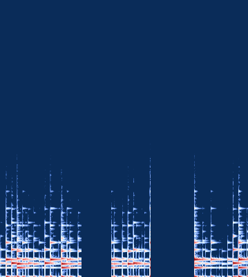
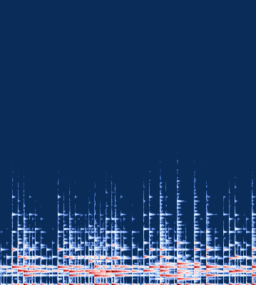
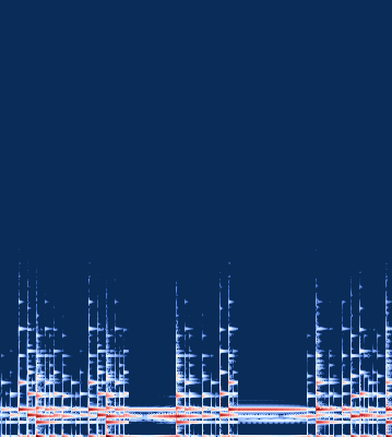
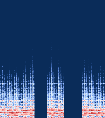
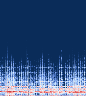
Analogously to the removal of eyes from a face, we consider the inference problem of filling in gaps in a piece of music. In this situation we will give significant weight to the evidence present, preferring to maintain the original signal where possible. It will also generally be advantageous to pick relatively wide memory factors (10-20 spectrogram pixels) to maximize the connection between the newly created signal and the original signal it is adjacent to. For example spectrograms for a reconstruction problem, see Fig. 5.

(a) Original

(b) Evidence

(c) Memory table soln.

(d) Subspace solution

Figure 5: An example output of an MFN on music with missing evidence. Run with $10$ pixel wide factors covering the entire frequency range, with $5$ hidden variables for the subspace factors. Updates were done in serial fashion. Evidence is given weight $20$ with memory factors given weight $1$. The memory table solution had mean square error 16.258 and the subspace solution had mean square error 7.130.

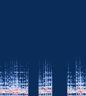
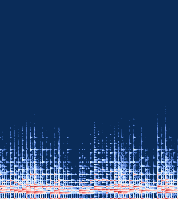
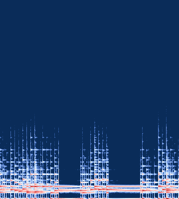
For constructing missing music, memory tables have significantly better properties than subspace factors in our testing. The memory table network selects full notes or sequences of notes and attempts to choose those that fit best with the surrounding music, whereas subspace factors generally match the dominant frequencies of the surrounding music but do not recreate the shape of notes, rather creating a sort of flat buzz, often with a volume spike. We believe part of the reason for this behavior is that the subspace factors are trained on a variety of shifts in time of a note and rather than being forced to choose between these shifts are able to combine them, creating smoother, blended sections of spectrogram that are quite unlike the patterns of notes in the training set.

6.2.4 Noisy music

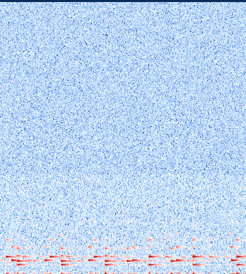
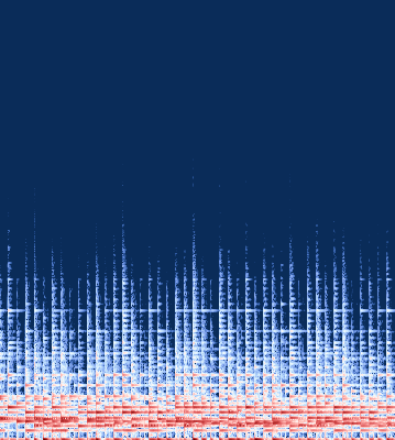
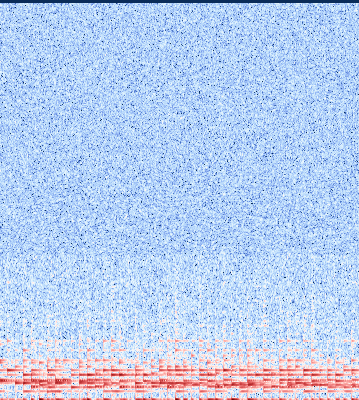
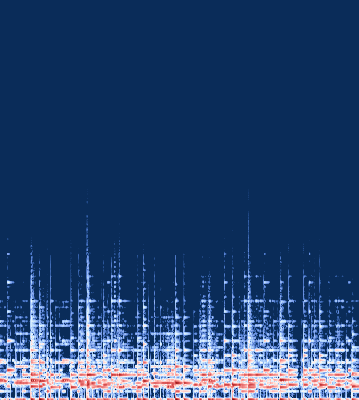
Another problem we consider is that of removing noise from a music sample. To simulate this problem we add normal random noise to our test sample. Because many regions of the spectrogram have value zero in the absence of noise, if evidence is given any significant weight relative to memory factors a certain degree of noise will still be present at the end of the algorithm. To combat this effect we run PMP twice, first with a large weight on the evidence and no votes from factors and then again with very little weight for the evidence but taking the final votes of the factors as the initial votes in the second run. This allows factors to take advantage of the evidence while not allowing it to dominate. Because factors primarily need to match the signal underneath the noise rather than coordinating over time intervals, we use very narrow factors (2 pixels) for noise problems.

(a) Original

(b) Evidence

(c) Memory table soln.

(d) Subspace solution

Figure 6: An example output of an MFN on music with noisy evidence. Run with $2$ pixel wide factors covering the entire frequency range, with 20 hidden variables for the subspace factors. Updates were done in serial fashion. Evidence is originally given weight $20$ with memory factors given weight $1$, with evidence weight set to $0.01$ for the second run initialized with the final factor votes of the first. The memory table solution had mean square error 10.386 and the subspace solution had mean square error 1.212.

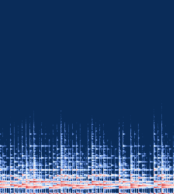
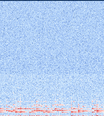
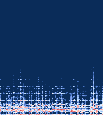
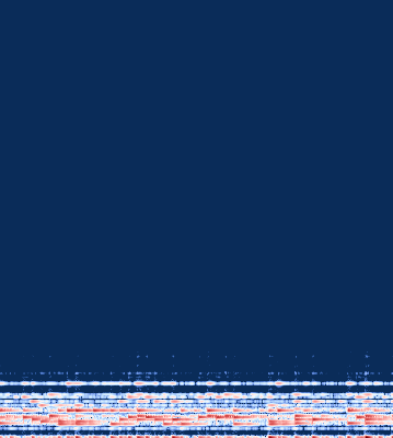
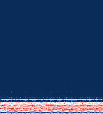
An example of a noisy music problem can be seen in Fig. 6. Again we see that memory tables are better able to maintain the rich structure of notes, though subspace factors do maintain much more of the structure of music than they did when attempting to create stretches of it, and are better able to exactly match the main structures than memory tables, which must try to find matching notes among their memories. Combining these notes from different training samples results in a somewhat more disjointed reconstruction, whereas subspace factors are somewhat fuzzier but smoother.

6.2.5 Results summary

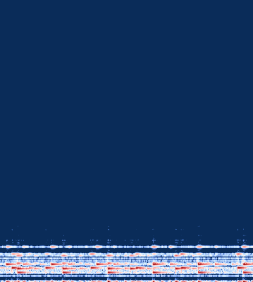
We ran PMP with the described settings for the two problems described above on each of the 20 test clips, computing the mean square error of the spectrogram pixel values. Statistics summarizing the results are presented in Table 2, and images for the best and worst examples of each problem are available in Appendix B.

Table 2: Mean Square Error Result Summary for Tests of Problems Described in Fig. 5 and 6

Problem Type	Factor Type	Mean	Median	Best	Worst
Sections Removed	Subspace	8.248	7.270	3.712	20.366
Sections Removed	Memory Table	14.025	12.835	8.205	28.042
Noisy Evidence	Subspace	1.459	1.238	0.635	4.303
Noisy Evidence	Memory Table	13.100	10.399	4.932	42.328

6.3 Handwritten digit classification

We now demonstrate the use of label variables and mixed-variable factors by using memory table MFNs to classify handwritten digits. We use the MNIST dataset LeCun et al. consisting of 60,000 training examples of $28\times 28$ grayscale images with correct classifications and 10,000 test images with no classification.

We work with $32\times 32$ images, in which the original images have been centered, in order to facilitate a hierarchy of pixel and label variables. In addition to $32^{2}$ level-0 variables representing the image’s pixels, there are $16^{2}$ hidden level-1 variables corresponding to a lower-resolution version of the same image, $8^{2}$ hidden level-2 variables corresponding to an even lower resolution version, and $4^{2}$ hidden level-3 variables representing the entire image. A hierarchy of label variables exists in parallel to the hierarchy of pixel variables, with $15^{2}$ level-0 variables, $7^{2}$ level-1 variables, $3^{2}$ level-2 variables, and a single level-3 variable characterizing the entire image. The pixel variables are integer variables with linear cost and weights of 1, while the label variables use an indicator cost as described in Section 4.3 with weights of 32. The label variables have a higher weight than the pixel variables both because there are fewer of them and because the natural scale of a mismatch is lower.

This hierarchy has two useful properties. Firstly, it allows locally inferred labels to be synthesized into one global label which can then be read off as the classification of the entire image. Secondly, it provides a “fast lane” for information to propagate from one part of the image to a more remote part. Inferences about pixels or labels can flow up and down the hierarchy in a faster way than if they had to linearly diffuse through the network.

The network hierarchy is constructed in the following manner. Each factor at level $n$ is connected to $8^{2}$ pixel variables and $3^{2}$ label variables of level $n$, as well as to $4^{2}$ pixel variables and 1 label variable of level $n+1$. A sample set of variables connected to a single memory table factor is shown in Fig. 7.

When a training example is presented to the system, all label variables are set to the correct label and all hidden pixel variables are set to the average of the pixel values in the corresponding $2\times 2$ patch of the image at the next lower level. Every memory in each memory table thus is filled with specified values.

Figure 7: All 90 variables connected to a sample memory table factor at level 1. 64 variables are a high-resolution representation of an $8\times 8$ region, 16 are a lower-resolution representation of the same region, 9 are labels correlated with $4\times 4$ subregions of the high-resolution image, and one is a label correlated with the entire region of the low-resolution image.

At testing time, the hidden pixel and label variables are not connected to evidence factors; they only acquire values as a result of being voted on by memory table factors. A level-0 factor that thinks that a group of pixels is characteristic of a 4 will cast votes for its neighboring level-1 pixel variables with a blurred version of its memory and cast a vote of 4 for its neighboring level-1 label variable. Factors pay a mismatch cost for disagreeing both with pixel variables and with label variables, and thus a factor that isn’t sure whether it is looking at a 4 or a 9 may be swayed by the fact that a neighboring factor has cast a vote for the label 4. When the algorithm has converged, we classify the image according to the single label at the top of the hierarchy.

This simple Memory Factor Network is sufficient to classify the 10,000 test images of the MNIST data set with 96.15% accuracy when run with a single factor voting at a time, and 96.41% accuracy when using simultaneous votes of the top 10% of factors (see Section 3.3). On average the single-vote implementation required 78.7 iterations and 1148.9 opinion updates, while the simultaneous-vote implementation required 16.9 iterations and 687.2 opinion updates.

6.4 Restoration of corrupted images

A natural application for MFNs using memory tables is to reconstruct previously-seen images when presented with versions of them that have been corrupted by noise or erasure. We use a similar network to that of the face reconstruction application and for data we use the CIFAR-10 dataset of $32\times 32$ RGB images Krizhevsky (2009), containing 50,000 images. The provided labeling of the images is irrelevant to our problem.

After all 50,000 images are read, one of the previously-seen images is selected at random and has Gaussian noise applied to every color channel value of every pixel with a standard deviation of 40. In addition, a randomly-generated blob of 144 pixels is completely erased from the center of the image (providing no evidence). This image is then presented to the MFN, which restores the image to its original version, removing the applied noise and filling in the correct pixels of the erased region.

This application is particularly convenient because it has a quantitative metric for assessing the quality of the result; we simply measure the L1 distance between the computed image and the original. This makes it a natural choice for evaluating the effect of changes to the algorithm.

Thus, to assess the effects of simultaneous voting, we ran the PMP algorithm over 1000 test images using both the standard serial algorithm and the simultaneous voting version described in Section 3.3, running 10% of all factors every iteration. While the simultaneous voting version was less likely to reproduce the initial image exactly, its average error was comparable to that of the serial version. The serial version restored 91.9% of the images perfectly with an average total L1 error across all color channels of 895.1 (0.291 per pixel per channel), while the simultaneous voting version restored only 83.1% of the images perfectly but with an average total L1 error of 936.7 (0.305 per pixel per channel).

7 Conclusions and future work

We have introduced here a new approach to combining inference with learning from experience. Memory factor networks provide a simple way to store examples learned from experience, while proactive message passing using a confidence-based scheme for prioritizing factor updates gives a reliable way to converge to good optima of the memory factor network cost function.

We consider the algorithms and the applications demonstrated here to be just an initial foray into the possibilities raised by this approach. Thus, one might consider factor graphs that combined memory factor nodes with more conventional factor nodes that encoded known statistical dependencies or constraints. The PMP algorithm is well-suited to MFNs, but one might nevertheless consider using other approaches, such as those based on belief propagation or variational approaches Wainwright and Jordan (2008), or those based on the alternating directions method of multipliers Boyd et al. (2011); Derbinsky et al. (2013). There are many potential applications that one might attack with this approach, including just from computer vision the problems of inferring depth from single images, or motion from videos. Finally, an important open question is how well the approach described here can take advantage of massive amounts of data, as are often now available Halevy et al. (2009).

Appendix A: Derivation of opinion update for real variables with quadratic cost

In this section we derive the messages in the message-passing version of PMP for real variables and quadratic costs. Under these choices, (3) specializes to

$${o^{a}=\operatorname*{arg\,min}_{\bar{o}}\left\{\chi_{a}(\bar{o})+\sum_{i\in\mathcal{N}_{a}}\min_{x_{i}}\left[w_{i}^{a}(x_{i}-\bar{o}_{i})^{2}+\sum_{b\in\mathcal{N}_{i}^{\backslash a}}w_{i}^{b}(x_{i}-v_{i}^{b})^{2}\right]\right\}}.$$ (17)

where we recall the definition of $\mathcal{N}_{i}^{\backslash a}=(\mathcal{N}_{i}\backslash\{a\})\backslash\mathcal{A}$, originally made in (5).

We first optimize the choice of $x_{i}$ by taking the derivative with respect to $x_{i}$:

$$\bar{x}_{i}=\operatorname*{arg\,min}_{x}\left[w_{i}^{b}(x-\bar{o}_{i})^{2}+\sum_{b\in\mathcal{N}_{i}^{\backslash a}}w_{i}^{b}(x-v_{i}^{b})^{2}\right]=\frac{\bar{o}_{i}w_{i}^{a}+\sum_{b\in\mathcal{N}_{i}^{\backslash a}}v_{i}^{b}w_{i}^{b}}{\sum_{b\in\mathcal{N}_{i}}w_{i}^{b}}.$$

If we define $\hat{w}_{i}=\sum_{b\in\mathcal{N}_{i}\setminus\mathcal{A}}w_{i}^{b}$ then $\sum_{b\in\mathcal{N}_{i}^{\backslash a}}w_{i}^{b}=\hat{w}_{i}-w_{i}^{a}$. Multiplying and dividing the second term by $(\hat{w}_{i}-w_{i}^{a})$ we get

$$\bar{x}_{i}=\frac{w_{i}^{a}\bar{o}_{i}+\left(\hat{w}_{i}-w_{i}^{a}\right)\tilde{x}_{i}}{\hat{w}_{i}},$$

where

$$\tilde{x}_{i}=\operatorname*{arg\,min}_{x}\sum_{b\in\mathcal{N}_{i}^{\backslash a}}w_{i}^{b}(x-v_{i}^{b})^{2}=\frac{\sum_{b\in\mathcal{N}_{i}^{\backslash a}}v_{i}^{b}w_{i}^{b}}{\sum_{b\in\mathcal{N}_{i}^{\backslash a}}w_{i}^{b}}=\frac{\sum_{b\in\mathcal{N}_{i}^{\backslash a}}v_{i}^{b}w_{i}^{b}}{\hat{w}_{i}-w_{i}^{a}}$$ (18)

is the minimization of $x_{i}$ with respect solely to memory factors in $\mathcal{N}_{i}^{\backslash a}$. This is the same $\tilde{x}_{i}$ as was defined in Sec. 3.2.

We denote the cost associated with a particular variable $i\in\mathcal{N}_{a}$ for a given opinion $\bar{o}_{i}$ as $c(\bar{o}_{i})$. Then we have

$$c(\bar{o}_{i}) =w_{i}^{a}\left(\bar{x}_{i}-\bar{o}_{i}\right)^{2}+\sum_{b\in\mathcal{N}_{i}^{\backslash a}}w_{i}^{b}\left(\bar{x}_{i}-v_{i}^{b}\right)^{2}$$

$$=w_{i}^{a}\left(\frac{w_{i}^{a}\bar{o}_{i}+\left(\hat{w}_{i}-w_{i}^{a}\right)\tilde{x}_{i}}{\hat{w}_{i}}-\bar{o}_{i}\right)^{2}+\sum_{b\in\mathcal{N}_{i}^{\backslash a}}w_{i}^{b}\left(\frac{w_{i}^{a}\bar{o}_{i}+\left(\hat{w}_{i}-w_{i}^{a}\right)\tilde{x}_{i}}{\hat{w}_{i}}-v_{i}^{b}\right)^{2}$$

$$=\frac{w_{i}^{a}(\hat{w}_{i}-w_{i}^{a})^{2}}{\hat{w}_{i}^{2}}(\tilde{x}_{i}-\bar{o}_{i})^{2}+\frac{1}{\hat{w}_{i}^{2}}\bigg{(}\sum_{b\in\mathcal{N}_{i}^{\backslash a}}w_{i}^{b}\left(w_{i}^{a}\bar{o}_{i}+\left(\hat{w}_{i}-w_{i}^{a}\right)\tilde{x}_{i}-\hat{w}_{i}v_{i}^{b}\right)^{2}\bigg{)}$$

$$=\frac{w_{i}^{a}(\hat{w}_{i}-w_{i}^{a})^{2}}{\hat{w}_{i}^{2}}(\bar{o}_{i}^{2}-2\bar{o}_{i}\tilde{x}_{i})+\frac{1}{\hat{w}_{i}^{2}}\bigg{(}\sum_{b\in\mathcal{N}_{i}^{\backslash a}}w_{i}^{b}[(w_{i}^{a}\bar{o}_{i})^{2}+w_{i}^{a}\left(\hat{w}_{i}-w_{i}^{a}\right)\bar{o}_{i}\tilde{x}_{i}-w_{i}^{a}\hat{w}_{i}v_{i}^{b}\bar{o}_{i}]\bigg{)}+C,$$

where the constant term $C$ includes all the terms that are not a function of $\bar{o}$. We next simplify the sums over $b\in\mathcal{N}_{i}^{\backslash a}$ by recalling that $\sum_{b\in\mathcal{N}_{i}^{\backslash a}}w_{i}^{b}=(\hat{w}_{i}-w_{i}^{a})$ and that, from (18), $\sum_{b\in\mathcal{N}_{i}^{\backslash a}}w_{i}^{b}v_{i}^{b}=(\hat{w}_{i}-w_{i}^{a})\tilde{x}_{i}$. Hence,

$$c(\bar{o}_{i}) =\frac{w_{i}^{a}(\hat{w}_{i}-w_{i}^{a})^{2}}{\hat{w}_{i}^{2}}(\bar{o}_{i}^{2}-2\bar{o}_{i}\tilde{x}_{i})+\bar{o}_{i}^{2}\frac{(w_{i}^{a})^{2}\left(\hat{w}_{i}-w_{i}^{a}\right)}{\hat{w}_{i}^{2}}+\bar{o}_{i}\tilde{x}_{i}\frac{w_{i}^{a}\left(\hat{w}_{i}-w_{i}^{a}\right)^{2}}{\hat{w}_{i}^{2}}-\bar{o}_{i}\tilde{x}_{i}\frac{w_{i}^{a}\hat{w}_{i}(\hat{w}_{i}-w_{i}^{a})}{\hat{w}_{i}^{2}}+C$$

$$=\frac{w_{i}^{a}(\hat{w}_{i}-w_{i}^{a})}{\hat{w}_{i}}\left(\bar{o}_{i}^{2}-2\tilde{x}_{i}\bar{o}_{i}\right)+C,$$

where in the second equation a number of terms cancel. We substitute this result into (17) noting that the constant $C$ can be dropped and adding a constant to make $\left(\bar{o}_{i}^{2}-2\tilde{x}_{i}\bar{o}_{i}\right)$ a quadratic form. This yields the final form of our optimization,

$${o^{a}=\operatorname*{arg\,min}_{\bar{o}}\left\{\chi_{a}(\bar{o})+\sum_{i\in\mathcal{N}_{a}}\frac{w_{i}^{a}(\hat{w}_{i}-w_{i}^{a})}{\hat{w}_{i}}\left(\bar{o}_{i}-\tilde{x}_{i}\right)^{2}\right\}}.$$ (19)

Appendix B: Reconstruction results

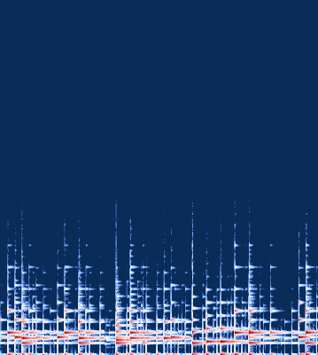
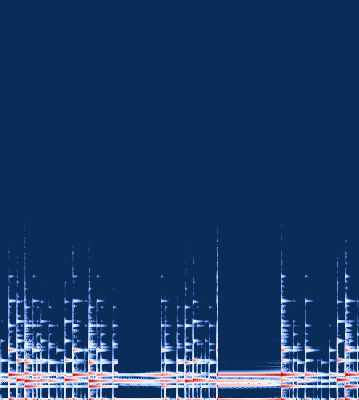
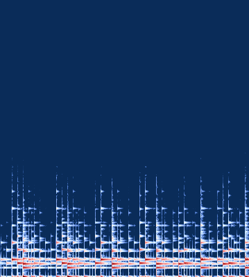
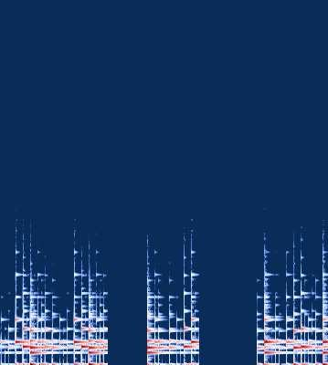
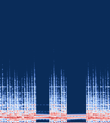
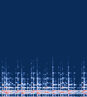
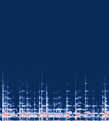
So that the reader can have a reasonable sense for the range of possible results, including the nature of artefacts obtained using proactive message passing on memory factor networks, we include here images of the best and worst solutions for a variety of problems and for each type of factor (memory table or subspace), first for reconstructing face images, and then reconstructing for music spectrograms.

Example	Original	Evidence	Memory Table Solution	Subspace Solution
Best Memory Table
			MSE: 0.0036	MSE: 0.0021
Best Subspace
			MSE: 0.0036	MSE: 0.0021
Worst Memory Table
			MSE: 0.0346	MSE: 0.0177
Worst Subspace
			MSE: 0.0138	MSE: 0.0210

Figure 8: Best and worst examples of eye reconstruction.

Example	Original	Evidence	Memory Table Solution	Subspace Solution
Best Memory Table
			MSE: 0.0023	MSE: 0.0027
Best Subspace
			MSE: 0.0034	MSE: 0.0026
Worst Memory Table
			MSE: 0.0111	MSE: 0.0056
Worst Subspace
			MSE: 0.0086	MSE: 0.0061

Figure 9: Best and worst examples of reconstructing with randomly missing evidence.

Example	Original	Evidence	Memory Table Solution	Subspace Solution
Best Memory Table
			MSE: 0.0005	MSE: 0.0004
Best Subspace
			MSE: 0.0005	MSE: 0.0004
Worst Memory Table
			MSE: 0.0058	MSE: 0.0047
Worst Subspace
			MSE: 0.0030	MSE: 0.0071

Figure 10: Best and worst examples of colorization.

Example	Original	Evidence	Memory Table Solution	Subspace Solution
Best Memory Table
			MSE: 0.0035	MSE: 0.0041
Best Subspace
			MSE: 0.0081	MSE: 0.0040
Worst Memory Table
			MSE: 0.0106	MSE: 0.0056
Worst Subspace
			MSE: 0.0073	MSE: 0.0064

Figure 11: Best and worst examples of reconstructing with noisy evidence.

Example	Original	Evidence	Memory Table Solution	Subspace Solution
Best Memory Table
			MSE: 8.205	MSE: 5.073
Best Subspace
			MSE: 10.341	MSE: 3.712
Worst Memory Table
			MSE: 28.042	MSE: 20.366
Worst Subspace
			MSE: 28.042	MSE: 20.366

Figure 12: Best and worst examples of reconstructing music with missing sections.

Example	Original	Evidence	Memory Table Solution	Subspace Solution
Best Memory Table
			MSE: 4.932	MSE: 0.635
Best Subspace
			MSE: 4.932	MSE: 0.635
Worst Memory Table
			MSE: 42.328	MSE: 4.304
Worst Subspace
			MSE: 42.328	MSE: 4.304

Figure 13: Best and worst examples of reconstructing music with noise added.

References

- (1) Otomata generative musical sequencer. http://www.earslap.com/page/otomata.html.
- (2) FEI face database. http://fei.edu.br/~cet/facedatabase.html.
- Baldi and Lu (2012) P. Baldi and Z. Lu. Complex-valued autoencoders. Neural Networks, 33:136–147, 2012.
- Boyd et al. (2011) S. Boyd, N. Parikh, E. Chu, B. Peleato, and J. Eckstein. Distributed optimization and statistical learning via the alternating direction method of multipliers. Foundations and Trends in Machine Learning, 3:1–122, 2011.
- Derbinsky et al. (2013) N. Derbinsky, J. Bento, V. Elser, and J. S. Yedidia. An improved three-weight message-passing algorithm. http://arxiv.org/pdf/1305.1961.pdf, 2013.
- Forney (2001) G. D. Forney. Codes on graphs: Normal realizations. IEEE Trans. Inform. Theory, 47(2):520–548, February 2001.
- Freeman et al. (2000) W. T. Freeman, E. C. Pasztor, and O. T. Carmichael. Learning low-level vision. Int. J. Computer Vision, 40(1):25–47, 2000.
- Freeman et al. (2002) W. T. Freeman, T. R. Jones, and E. C. Pasztor. Example-based super-resolution. IEEE Computer Graphics and Applications, 22:56–65, 2002.
- Halevy et al. (2009) A. Halevy, P. Norvig, and F. Pereira. The unreasonable effectiveness of data. IEEE Intelligent Systems, 24(2):8–12, 2009.
- Koller and Friedman (2009) D. Koller and N. Friedman. Probabilistic Graphical Models: Principles and Techniques. MIT Press, 2009.
- Krizhevsky (2009) A. Krizhevsky. Learning multiple layers of features from tiny images. Masters Thesis, University of Toronto, 2009.
- Kschischang et al. (2001) F. R. Kschischang, B. J. Frey, and H. Loeliger. Factor graphs and the sum-product algorithm. IEEE Trans. Inform. Theory, 47:498–519, February 2001.
- (13) Y. LeCun, C. Cortes, and C. J. C. Burge. The MNIST database of handwritten digits. http://yann.lecun.com/exdb/mnist/.
- Loeliger et al. (2007) H. Loeliger, J. Dauwels, J. Hu, S. Korl, L. Ping, and F. R. Kschischang. The factor graph approach to model-based signal processing. Proc. of the IEEE, 95(6):1295–1322, 2007.
- Mézard et al. (1987) M. Mézard, G. Parisi, and M. A. Virasoro. Spin Glass Theory and Beyond. World Scientific, 1987.
- Richardson and Urbanke (2008) T. J. Richardson and R. Urbanke. Modern Coding Theory. Cambridge University Press, 2008.
- Sudderth and Freeman (2008) E. Sudderth and W. T. Freeman. Signal and image processing with belief propagation. IEEE Signal Process. Mag., 25:114–141, March 2008.
- Wainwright and Jordan (2008) M. J. Wainwright and M. I. Jordan. Graphical models, exponential families, and variational inference. Foundations and Trends in Machine Learning, 1:1–305, 2008.
- Yedidia et al. (2005) J. S. Yedidia, W. T. Freeman, and Y. Weiss. Constructing free energy approximations and generalized belief propagation algorithms. IEEE Trans. Inform. Theory, 51(7):2282–2312, 2005.