Incremental Semiparametric Inverse Dynamics Learning

Abstract

This paper presents a novel approach for incremental semiparametric inverse dynamics learning. In particular, we consider the mixture of two approaches: Parametric modeling based on rigid body dynamics equations and nonparametric modeling based on incremental kernel methods, with no prior information on the mechanical properties of the system. This yields to an incremental semiparametric approach, leveraging the advantages of both the parametric and nonparametric models. We validate the proposed technique learning the dynamics of one arm of the iCub humanoid robot.

I INTRODUCTION

In order to control a robot a model describing the relation between the actuator inputs, the interactions with the world and bodies accelerations is required. This model is called the dynamics model of the robot. A dynamics model can be obtained from first principles in mechanics, using the techniques of rigid body dynamics (RBD) [1], resulting in a parametric model in which the values of physically meaningful parameters must be provided to complete the fixed structure of the model. Alternatively, the dynamical model can be obtained from experimental data using Machine Learning techniques, resulting in a nonparametric model.

Traditional dynamics parametric methods are based on several assumptions, such as rigidity of links or that friction has a simple analytical form, which may not be accurate in real systems. On the other hand, nonparametric methods based on algorithms such as Kernel Ridge Regression (KRR) [2, 3, 4], Kernel Regularized Least Squares (KRLS) [5] or Gaussian Processes [6] can model dynamics by extrapolating the input-output relationship directly from the available data. If a suitable kernel function is chosen, then the nonparametric model is a universal approximator which can account for the dynamics effects which are not considered by the parametric model. Still, nonparametric models have no prior knowledge about the target function to be approximated. Therefore, they need a sufficient amount of training examples in order to produce accurate predictions on the entire input space. If the learning phase has been performed offline, both approaches are sensitive to the variation of the mechanical properties over long time spans, which are mainly caused by temperature shifts and wear. Even the inertial parameters can change over time. For example if the robot grasps a heavy object, the resulting change in dynamics can be described by a change of the inertial parameters of the hand. A solution to this problem is to address the variations of the identified system properties by learning incrementally, continuously updating the model as long as new data becomes available. In this paper we propose a novel technique that joins parametric and nonparametric model learning in an incremental fashion.

TABLE I: Summary of related works on semiparametric or incremental robot dynamics learning.

Author, Year	Parametric	Nonparametric
Nguyen-Tuong, 2010 [7]	Batch	Batch
Gijsberts, 2011 [8]	-	Incremental
Tingfan Wu, 2012 [9]	Batch	Batch
De La Cruz, 2012 [10]	CAD∗	Incremental
Camoriano, 2015	Incremental	Incremental

^∗ In [10] the parametric part is used only for initializing the nonparametric model.

Classical methods for physics-based dynamics modeling can be found in [1]. These methods require to identify the mechanical parameters of the rigid bodies composing the robot [11, 12, 13, 14], which can then be employed in model-based control and state estimation schemes.

In [7] the authors present a learning technique which combines prior knowledge about the physical structure of the mechanical system and learning from available data with Gaussian Process Regression (GPR) [6]. A similar approach is presented in [9]. Both techniques require an offline training phase and are not incremental, limiting them to scenarios in which the properties of the system do not change significantly over time.

In [10] an incremental semiparametric robot dynamics learning scheme based on Locally Weighted Projection Regression (LWPR) [15] is presented, that is initialized using a linearized parametric model. However, this approach uses a fixed parametric model, that is not updated as new data becomes available. Moreover, LWPR has been shown to underperform with respect to other methods (e.g. [8]).

In [8], a fully nonparametric incremental approach for inverse dynamics learning with constant update complexity is presented, based on kernel methods [16] (in particular KRR) and random features [17]. The incremental nature of this approach allows for adaptation to changing conditions in time. The authors also show that the proposed algorithm outperforms other methods such as LWPR, GPR and Local Gaussian Processes (LGP) [18], both in terms of accuracy and prediction time. Nevertheless, the fully nonparametric nature of this approach undermines the interpretability of the inverse dynamics model.

In this work we propose a method that is incremental with fixed update complexity (as [8]) and semiparametric (as [7] and [9]). The fixed update complexity and prediction time are key properties of our method, enabling real-time performances. Both the parametric and nonparametric parts can be updated, as opposed to [10] in which only the nonparametric part is. A comparison between the existing literature and our incremental method is reported in Table I. We validate the proposed method with experiments performed on an arm of the iCub humanoid robot [19].

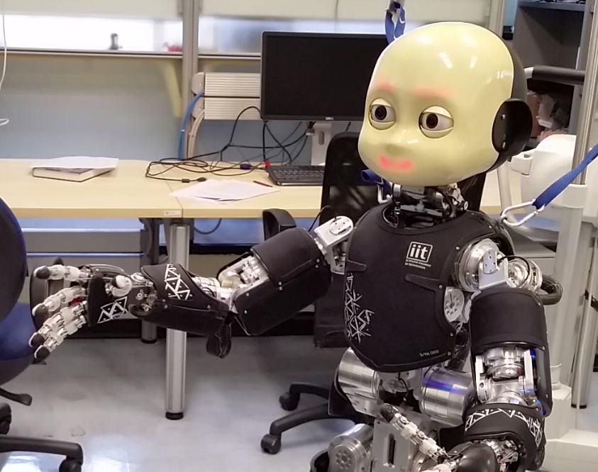
Figure 1: iCub learning its right arm dynamics.

The article is organized as follows. Section II introduces the existing techniques for parametric and nonparametric robot dynamics learning. In Section III, a complete description of the proposed semiparametric incremental learning technique is introduced. Section IV presents the validation of our approach on the iCub humanoid robotic platform. Finally, Section V summarizes the content of our work.

II BACKGROUND

II-A Notation

The following notation is used throughout the paper.

• The set of real numbers is denoted by $\mathbb{R}$. Let $\mathbf{u}$ and $\mathbf{v}$ be two $n$-dimensional column vectors of real numbers (unless specified otherwise), i.e. $\mathbf{u},\mathbf{v}\in\mathbb{R}^{n}$, their inner product is denoted as $\mathbf{u}^{\top}\mathbf{v}$, with “$\top$” the transpose operator.

• The Frobenius norm of either a vector or a matrix of real numbers is denoted by $\|\cdot\|$.

• $I_{n}\in\mathbb{R}^{n\times n}$ denotes the identity matrix of dimension $n$; $0_{n}\in\mathbb{R}^{n}$ denotes the zero column vector of dimension $n$; $0_{n\times m}\in\mathbb{R}^{n\times m}$ denotes the zero matrix of dimension $n\times m$.

II-B Parametric Models of Robot Dynamics

Robot dynamics parametric models are used to represent the relation connecting the geometric and inertial parameters with some dynamic quantities that depend uniquely on the robot model. A typical example is obtained by writing the robot inverse dynamics equation in linear form with respect to the robot inertial parameters $\bm{\pi}$:

$$\bm{\tau}=M(\mathbf{q})\mathbf{\ddot{q}}+C(\mathbf{q},\mathbf{\dot{q}})\mathbf{\dot{q}}+g(\mathbf{q})=\Phi(\mathbf{x})\bm{\pi},$$ (1)

where: $\mathbf{q}\in\mathbb{R}^{n_{dof}}$ is the vector of joint positions, $\bm{\tau}\in\mathbb{R}^{n_{dof}}$ is the vector of joint torques, $\bm{\pi}\in\mathbb{R}^{n_{p}}$ is the vector of the identifiable (base) inertial parameters [1], $\Phi(\mathbf{x})\in\mathbb{R}^{n_{dof}\times n_{p}}$ is the “regressor”, i.e. a matrix that depends only on the robot kinematic parameters. In the rest of the paper we will indicate with $\mathbf{x}$ the triple given by $(\mathbf{q},\mathbf{\dot{q}},\mathbf{\ddot{q}})$. Other parametric models write different measurable quantities as a product of a regressor and a vector of parameters, for example the total energy of the robot [20], the istantaneous power provided to the robot [21], the sum of all external forces acting on the robot [22] or the center of pressure of the ground reaction forces [23]. Regardless of the choice of the measured variable $\mathbf{y}$, the structure of the regressor is similar:

$$\mathbf{y}=\Phi(\mathbf{q},\mathbf{\dot{q}},\mathbf{\ddot{q}})\bm{\pi}=\Phi(\mathbf{x})\bm{\pi},$$ (2)

where $\mathbf{y}\in\mathbb{R}^{t}$ is the measured quantity.

The $\bm{\pi}$ vector is composed of certain linear combinations of the inertial parameters of the links, the base inertial parameters [24]. In particular, the inertial parameters of a single body are the mass $m$, the first moment of mass $m\mathbf{c}\in\mathbb{R}^{3}$ expressed in a body fixed frame and the inertia matrix $I\in\mathbb{R}^{3\times 3}$ expressed in the orientation of the body fixed frame and with respect to its origin.

In parametric modeling of robot dynamics, the regressor structure depends on the kinematic parameters of the robot, that are obtained from CAD models of the robot through kinematic calibration techniques. Similarly, the inertial parameters $\bm{\pi}$ can also be obtained from CAD models of the robot, however these models may be unavailable (for example) because the manufacturer of the robot does not provide them. In this case the usual approach is to estimate $\bm{\pi}$ from experimental data [14]. To do that, given $n$ measures of the measured quantity $\mathbf{y}_{i}$ (with $i=1\dots n$), stacking (2) for the $n$ samples it is possible to write:

$$\begin{bmatrix}\mathbf{y}_{1}\\ \mathbf{y}_{2}\\ \vdots\\ \mathbf{y}_{n}\end{bmatrix}=\begin{bmatrix}\Phi(\mathbf{x}_{1})\\ \Phi(\mathbf{x}_{2})\\ \vdots\\ \Phi(\mathbf{x}_{n})\end{bmatrix}\bm{\pi}.$$ (3)

This equation can then be solved in least squares (LS) sense to find an estimate $\hat{\bm{\pi}}$ of the base inertial parameters. Given the training trajectories it is possible that not all parameters in $\bm{\pi}$ can be estimated well as the problem in (3) can be ill-posed, hence this equation is usually solved as a Regularized Least Squares (RLS) problem. Defining

$$\overline{\mathbf{y}}_{n}=\begin{bmatrix}\mathbf{y}_{1}\\ \mathbf{y}_{2}\\ \vdots\\ \mathbf{y}_{n}\end{bmatrix},\hskip 10.00002pt\overline{\bm{\Phi}}_{n}=\begin{bmatrix}\Phi(\mathbf{x}_{1})\\ \Phi(\mathbf{x}_{2})\\ \vdots\\ \Phi(\mathbf{x}_{n})\end{bmatrix},$$

the RLS problem that is solved for the parametric identification is:

$$\hat{\bm{\pi}}=\operatorname*{\arg\!\min}\limits_{\bm{\pi}\in\mathbb{R}^{n_{p}}}\left(\|\overline{\bm{\Phi}}_{n}\bm{\pi}-\overline{\mathbf{y}}_{n}\|^{2}+\lambda\|\bm{\pi}\|^{2}\right),\lambda>0.$$ (4)

II-C Nonparametric Modeling with Kernel Methods

Consider a probability distribution $\rho$ over the probability space $\mathcal{X}\times\mathcal{Y}$, where $\mathcal{X}\subseteq\mathbb{R}^{d}$ is the input space (the space of the $d$ measured attributes) and $\mathcal{Y}\subseteq\mathbb{R}^{t}$ is the output space (the space of the $t$ outputs to be predicted). In a nonparametric modeling setting, the goal is to find a function $f^{*}:\mathcal{X}\rightarrow\mathcal{Y}$ belonging to a set of measurable functions $\mathcal{H}$, called hypothesis space, such that

$$f^{*}=\operatorname*{\arg\!\min}\limits_{f\in\mathcal{H}}\underbrace{\int_{\mathcal{X}\times\mathcal{Y}}\ell(f(\mathbf{x}),\mathbf{y})d\rho(\mathbf{x},\mathbf{y})}_{\mathcal{E}(f)},$$ (5)

where $\mathbf{x}\in\mathcal{X}$ are row vectors, $\mathbf{y}\in\mathcal{Y}$, $\mathcal{E}(f)$ is called expected risk and $\ell(f(\mathbf{x}),\mathbf{y})$ is the loss function. In the rest of this work, we will consider the squared loss $\ell(f(\mathbf{x}),\mathbf{y})=\|f(\mathbf{x})-\mathbf{y}\|^{2}$. Note that the distribution $\rho$ is unknown, and that we assume to have access to a discrete and finite set of measured data points $S=\{\mathbf{x}_{i},\mathbf{y}_{i}\}_{i=1}^{n}$ of cardinality $n$, in which the points are independently and identically distributed (i.i.d.) according to $\rho$.
In the context of kernel methods [16], $\mathcal{H}$ is a reproducing kernel Hilbert space (RKHS). An RKHS is a Hilbert space of functions such that $\exists k:\mathcal{X}\times\mathcal{X}\rightarrow\mathbb{R}$ for which the following properties hold:

1. $\forall\mathbf{x}\in\mathcal{X}\quad k_{\mathbf{x}}(\cdot)=k(\mathbf{x},\cdot)\in\mathcal{H}$

2. $g(\mathbf{x})=\left\langle g,k_{\mathbf{x}}\right\rangle_{\mathcal{H}}\forall g\in\mathcal{H},\mathbf{x}\in\mathcal{X}$ ,

where $\left\langle\cdot,\cdot\right\rangle_{\mathcal{H}}$ indicates the inner product in $\mathcal{H}$. The function $k$ is a reproducing kernel, and it can be shown to be symmetric positive definite (SPD). We also define the kernel matrix $K\in\mathbb{R}^{n\times n}\quad s.t.\quad K_{i,j}=k(\mathbf{x}_{i},\mathbf{x}_{j})$, which is symmetric and positive semidefinite (SPSD) $\forall\mathbf{x}_{i},\mathbf{x}_{j}\in\mathcal{X}$, with $i,j\in\{1,\ldots,n\},n\in\mathbb{N}^{+}$.

The optimization problem outlined in (5) can be approached empirically by means of many different algorithms, among which one of the most widely used is Kernel Regularized Least Squares (KRLS) [3, 5]. In KRLS, a regularized solution $\hat{f}_{\lambda}:\mathcal{X}\rightarrow\mathcal{Y}$ is found solving

$$\hat{f}_{\lambda}=\operatorname*{\arg\!\min}\limits_{f\in\mathcal{H}}\left(\sum_{i=1}^{n}\|f(\mathbf{x}_{i})-\mathbf{y}_{i}\|^{2}+\lambda\|f\|_{\mathcal{H}}^{2}\right),\lambda>0,$$ (6)

where $\lambda$ is called regularization parameter. The solution to (6) exists and is unique. Following the representer theorem [16], the solution can be conveniently expressed as

$$\hat{f}_{\lambda}(\mathbf{x})=\sum_{i=1}^{n}\bm{\alpha}_{i}k(\mathbf{x}_{i},\mathbf{x})$$ (7)

with $\bm{\alpha}=(K+\lambda I_{n})^{-1}Y\in\mathbb{R}^{n\times t}$, $\bm{\alpha}_{i}$ $i$-th row of $\bm{\alpha}$ and $Y=\left[\mathbf{y}^{\top}_{1},\ldots,\mathbf{y}^{\top}_{n}\right]^{\top}$. It is therefore necessary to invert and store the kernel matrix $K\in\mathbb{R}^{n\times n}$, which implies $O(n^{3})$ and $O(n^{2})$ time and memory complexities, respectively. Such complexities render the above-mentioned KRLS approach prohibitive in settings where $n$ is large, including the one treated in this work. This limitation can be dealt with by resorting to approximated methods such as random features, which will now be described.

II-C1 Random Feature Maps for Kernel Approximation

The random features approach was first introduced in [17], and since then is has been widely applied in the field of large-scale Machine Learning. This approach leverages the fact that the kernel function can be expressed as

$$k(\mathbf{x},\mathbf{x}^{\prime})=\left\langle\phi(\mathbf{x}),\phi(\mathbf{x}^{\prime})\right\rangle_{\mathcal{H}},$$ (8)

where $\mathbf{x},\mathbf{x}^{\prime}\in\mathcal{X}$ are row vectors, $\phi:\mathbb{R}^{d}\rightarrow\mathbb{R}^{p}$ is a feature map associated with the kernel, which maps the input points from the input space $\mathcal{X}$ to a feature space of dimensionality $p\leq+\infty$, depending on the chosen kernel. When $p$ is very large, directly computing the inner product as in (8) enables the computation of the solution, as we have seen for KRLS. However, $K$ can become too cumbersome to invert and store as $n$ grows. A random feature map $\tilde{\phi}:\mathbb{R}^{d}\rightarrow\mathbb{R}^{D}$, typically with $D\ll p$, directly approximates the feature map $\phi$, so that

$$k(\mathbf{x},\mathbf{x}^{\prime})=\left\langle\phi(\mathbf{x}),\phi(\mathbf{x}^{\prime})\right\rangle_{\mathcal{H}}\approx\tilde{\phi}(\mathbf{x})\tilde{\phi}(\mathbf{x}^{\prime})^{\top}.$$ (9)

$D$ can be chosen according to the desired approximation accuracy, as guaranteed by the convergence bounds reported in [17, 25]. In particular, we will use random Fourier features for approximating the Gaussian kernel

$$k(\mathbf{x},\mathbf{x}^{\prime})=e^{-\frac{\|\mathbf{x}-\mathbf{x}^{\prime}\|^{2}}{2\sigma^{2}}}.$$ (10)

The approximated feature map in this case is $\tilde{\phi}(\mathbf{x})=\left[e^{i\mathbf{x}\bm{\omega}_{1}},\ldots,e^{i\mathbf{x}\bm{\omega}_{D}}\right]$, where

$$\bm{\omega}\sim p(\bm{\omega})=(2\pi)^{-\frac{D}{2}}e^{-\frac{\|\bm{\omega}\|^{2}}{2\sigma^{2}}},$$ (11)

with $\bm{\omega}\in\mathbb{R}^{d}$ column vector. The fundamental theoretical result on which random Fourier features approximation relies is Bochner’s Theorem [26]. The latter states that if $k(\mathbf{x},\mathbf{x}^{\prime})$ is a shift-invariant kernel on $\mathbb{R}^{d}$, then $k$ is positive definite if and only if its Fourier transform $p(\omega)\geq 0$. If this holds, by the definition of Fourier transform we can write

$$k(\mathbf{x},\mathbf{x}^{\prime})=k(\mathbf{x}-\mathbf{x}^{\prime})=\int_{\mathbb{R}^{d}}p(\bm{\omega})e^{i(\mathbf{x}-\mathbf{x}^{\prime})\bm{\omega}}d\bm{\omega},$$ (12)

which can be approximated by performing an empirical average as follows:

$$\begin{array}[]{r@{}l}k(\mathbf{x}-\mathbf{x}^{\prime})&{}=\mathbb{E}_{\bm{\omega}\sim p}\left[e^{i(\mathbf{x}-\mathbf{x}^{\prime})\bm{\omega}}\right]\approx\\ &{}\approx\frac{1}{D}\sum_{k=1}^{D}e^{i(\mathbf{x}-\mathbf{x}^{\prime})\bm{\omega}}=\tilde{\phi}(\mathbf{x})\tilde{\phi}(\mathbf{x}^{\prime})^{\top}.\end{array}$$ (13)

Therefore, it is possible to map the input data as $\tilde{\mathbf{x}}=\tilde{\phi}(\mathbf{x})\in\mathbb{R}^{D}$, with $\tilde{\mathbf{x}}$ row vector, to obtain a nonlinear and nonparametric model of the form

$$\tilde{f}(\mathbf{x})=\tilde{\mathbf{x}}\tilde{W}\approx\hat{f}_{\lambda}(\mathbf{x})=\sum_{i=1}^{n}\bm{\alpha}_{i}k(\mathbf{x}_{i},\mathbf{x})$$ (14)

approximating the exact kernelized solution $\hat{f}_{\lambda}(\mathbf{x})$, with $\tilde{W}\in\mathbb{R}^{D\times t}$. Note that the approximated model is nonlinear in the input space, but linear in the random features space. We can therefore introduce the regularized linear regression problem in the random features space as follows:

$$\tilde{W}^{\lambda}=\operatorname*{\arg\!\min}\limits_{\tilde{W}\in\mathbb{R}^{d\times t}}\left(\|\tilde{X}\tilde{W}-Y\|^{2}+\lambda\|\tilde{W}\|^{2}\right),\lambda>0,$$ (15)

where $\tilde{X}\in\mathbb{R}^{n\times D}$ is the matrix of the training inputs where each row has been mapped by $\tilde{\phi}$. The main advantage of performing a random feature mapping is that it allows us to obtain a nonlinear model by applying linear regression methods. For instance, Regularized Least Squares (RLS) can compute the solution $\tilde{W}^{\lambda}$ of (15) with $O(nD^{2})$ time and $O(D^{2})$ memory complexities. Once $\tilde{W}^{\lambda}$ is known, the prediction $\hat{\mathbf{y}}\in\mathbb{R}^{1\times t}$ for a mapped sample $\tilde{\mathbf{x}}$ can be computed as $\hat{\mathbf{y}}=\tilde{\mathbf{x}}\tilde{W}^{\lambda}$.

II-D Regularized Least Squares

Let $Z\in\mathbb{R}^{a\times b}$ and $U\in\mathbb{R}^{a\times c}$ be two matrices of real numbers, with $a,b,c\in\mathbb{N}^{+}$. The Regularized Least Squares (RLS) algorithm computes a regularized solution $W^{\lambda}\in\mathbb{R}^{b\times c}$ of the potentially ill-posed problem $ZW=U$, enforcing its numerical stability. Considering the widely used Tikhonov regularization scheme, $W^{\lambda}\in\mathbb{R}^{b\times c}$ is the solution to the following problem:

$$W^{\lambda}=\operatorname*{\arg\!\min}\limits_{W\in\mathbb{R}^{b\times c}}\underbrace{\left(\|ZW-U\|^{2}+\lambda\|W\|^{2}\right)}_{J(W,\lambda)},\quad\lambda>0,$$ (16)

where $\lambda$ is the regularization parameter. By taking the gradient of $J(W,\lambda)$ with respect to $W$ and equating it to zero, the minimizing solution can be written as

$$W^{\lambda}=(Z^{\top}Z+\lambda I_{b})^{-1}Z^{\top}U.$$ (17)

Both the parametric identification problem (4) and the nonparametric random features problem (15) are specific instances of the general problem (16).

In particular, the parametric problem (4) is equivalent to (16) with:

$$W^{\lambda}=\hat{\bm{\pi}},\hskip 10.00002ptZ=\overline{\Phi}_{n},\hskip 10.00002ptU=\overline{\mathbf{y}}_{n}$$

while the random features learning problem (15) is equivalent to (16) with:

$$W^{\lambda}=\tilde{W}^{\lambda},\hskip 10.00002ptZ=\tilde{X},\hskip 10.00002ptU=Y.$$

Hence, both problems for a given set of $n$ samples can be solved applying (17).

II-E Recursive Regularized Least Squares (RRLS) with Cholesky Update

In scenarios in which supervised samples become available sequentially, a very useful extension of the RLS algorithm consists in the definition of an update rule for the model which allows it to be incrementally trained, increasing adaptivity to changes of the system properties through time. This algorithm is called Recursive Regularized Least Squares (RRLS). We will consider RRLS with the Cholesky update rule [27], which is numerically more stable than others (e.g. the Sherman-Morrison-Woodbury update rule). In adaptive filtering, this update rule is known as the QR algorithm [28].

Let us define $A=Z^{\top}Z+\lambda I_{b}$ with $\lambda>0$ and $B=Z^{\top}U$. Our goal is to update the model (fully described by $A$ and $B$) with a new supervised sample $(\mathbf{z}_{k+1},\mathbf{u}_{k+1})$, with $\mathbf{z}_{k+1}\in\mathbb{R}^{b}$, $\mathbf{u}_{k+1}\in\mathbb{R}^{c}$ row vectors.

Consider the Cholesky decomposition $A=R^{\top}R$. It can always be obtained, since $A$ is positive definite for $\lambda>0$. Thus, we can express the update problem at step $k+1$ as:

$$\begin{array}[]{r@{}l}A_{k+1}&{}=R^{\top}_{k+1}R_{k+1}\\ &{}=A_{k}+\mathbf{z}_{k+1}^{\top}\mathbf{z}_{k+1}\\ &{}=R^{\top}_{k}R_{k}+\mathbf{z}_{k+i}^{\top}\mathbf{z}_{k+1},\end{array}$$ (18)

where $R$ is full rank and unique, and $R_{0}=\sqrt{\lambda}I_{b}$.
By defining

$$\tilde{R}_{k}=\left[\begin{array}[]{c}R_{k}\\ \mathbf{z}_{k+1}\end{array}\right]\in\mathbb{R}^{b+1\times b},$$ (19)

we can write $A_{k+1}=\tilde{R}_{k}^{\top}\tilde{R}_{k}$. However, in order to compute $R_{k+1}$ from the obtained $A_{k+1}$ it would be necessary to recompute its Cholesky decomposition, requiring $O(b^{3})$ computational time. There exists a procedure, based on Givens rotations, which can be used to compute $R_{k+1}$ from $\tilde{R}_{k}$ with $O(b^{2})$ time complexity. A recursive expression can be obtained also for $B_{k+1}$ as follows:

$$\begin{array}[]{r@{}l}B_{k+1}&{}=Z_{k+1}^{\top}U_{k+1}\\ &{}=Z_{k}^{\top}U_{k}+\mathbf{z}_{k+1}^{\top}\mathbf{u}_{k+1}.\end{array}$$ (20)

Once $R_{k+1}$ and $B_{k+1}$ are known, the updated weights matrix $W_{k}$ can be obtained via back and forward substitution as

$$W_{k+1}=R_{k+1}\setminus(R^{\top}_{k+1}\setminus B_{k+1}).$$ (21)

The time complexity for updating $W$ is $O(b^{2})$.

As for RLS, the RRLS incremental solution can be applied to both the parametric (4) and nonparametric with random features (15) problems, assuming $\lambda>0$. In particular, RRLS can be applied to the parametric case by noting that the arrival of a new sample $\left(\Phi_{r},\mathbf{y}_{r}\right)$ adds $t$ rows to $Z_{k}=\overline{\Phi}_{r-1}$ and $U_{k}=\overline{\mathbf{y}}_{r-1}$. Consequently, the update of $A$ must be decomposed in $t$ update steps using (20). For each one of these $t$ steps we consider only one row of $\Phi_{r}$ and $\mathbf{y}^{\top}_{r}$, namely:

$$\mathbf{z}_{k+i}=(\Phi_{r})_{i},\hskip 10.00002pt\mathbf{u}_{k+i}=(\mathbf{y}^{\top}_{r})_{i},\hskip 10.00002pti=1\dots t$$

where $(V)_{i}$ is the $i$-th row of the matrix $V$.

For the nonparametric random features case, RRLS can be simply applied with:

$$\mathbf{z}_{k+1}=\tilde{\mathbf{x}}_{r},\hskip 10.00002pt\mathbf{u}_{k+1}=\mathbf{y}_{r}.$$

where $\left(\tilde{\mathbf{x}}_{r},\mathbf{y}_{r}\right)$ is the supervised sample which becomes available at step $r$.

III SEMIPARAMETRIC INCREMENTAL DYNAMICS LEARNING

\begin{overpic}[width=390.25534pt]{figures/SemiParametricBlockDiagram8-1.eps} \put(2.5,16.0){$\mathbf{q}$} \put(2.5,12.5){$\mathbf{\dot{q}}$} \put(2.5,9.0){$\mathbf{\ddot{q}}$} \put(2.5,3.3){$\bm{f}$} \put(2.5,1.1){$\bm{\tau}$} \put(9.0,13.9){$\mathbf{x}$} \put(9.0,3.9){$\mathbf{y}$} \put(27.7,14.2){\footnotesize$\Phi(\mathbf{x})$} \put(39.73,24.0){$\hat{\bm{\pi}}$} \put(54.0,13.9){$\hat{\mathbf{y}}$} \put(75.2,12.5){$\tilde{\mathbf{x}}$} \put(92.2,12.5){$\triangle\tilde{\mathbf{y}}$} \put(50.0,4.5){$-$} \put(49.0,1.0){$+$} \put(58.0,4.0){$\triangle\mathbf{y}$} \put(97.6,11.1){$+$} \put(97.8,24.0){$\tilde{\mathbf{y}}$} \end{overpic}

Figure 2: Block diagram displaying the functioning of the proposed prioritized semiparametric inverse dynamics estimator. $\bm{f}$ and $\bm{\tau}$ indicate measured force and torque components, concatenated in the measured output vector $\mathbf{y}$. The parametric part is composed of the RBD regressor generator and of the parametric estimator based on RRLS. Its outputs are the estimated parameters $\hat{\bm{\pi}}$ and the predicted output $\hat{\mathbf{y}}$. The nonparametric part maps the input to the random features space with the Random Features Mapper block, and the RFRRLS estimator predicts the residual output $\triangle\tilde{\mathbf{y}}$, which is then added to the parametric prediction $\hat{\mathbf{y}}$ to obtain the semiparametric prediction $\tilde{\mathbf{y}}$.

We propose a semiparametric incremental inverse dynamics estimator, designed to have better generalization properties with respect to fully parametric and nonparametric ones, both in terms of accuracy and convergence rates. The estimator, whose functioning is illustrated by the block diagram in Figure 2, is composed of two main parts. The first one is an incremental parametric estimator taking as input the rigid body dynamics regressors $\Phi(x)$ and computing two quantities at each step:

• An estimate $\hat{\mathbf{y}}$ of the output quantities of interest

• An estimate $\hat{\bm{\pi}}$ of the base inertial parameters of the links composing the rigid body structure

The employed learning algorithm is RRLS. Since it is supervised, during the model update step the measured output $\mathbf{y}$ is used by the learning algorithm as ground truth. The parametric estimation is performed in the first place, and it is independent of the nonparametric part. This property is desirable in order to give priority to the identification of the inertial parameters $\bm{\pi}$. Moreover, being the estimator incremental, the estimated inertial parameters $\hat{\bm{\pi}}$ adapt to changes in the inertial properties of the links, which can occur if the end-effector is holding a heavy object. Still, this adaptation cannot address changes in nonlinear effects which do not respect the rigid body assumptions.
The second estimator is also RRLS-based, fully nonparametric and incremental. It leverages the approximation of the kernel function via random Fourier features, as outlined in Section II-C1, to obtain a nonlinear model which can be updated incrementally with constant update complexity $O(D^{2})$, where $D$ is the dimensionality of the random feature space (see Section II-E). This estimator receives as inputs the current vectorized $\mathbf{x}$ and $\hat{\mathbf{y}}$, normalized and mapped to the random features space approximating an infinite-dimensional feature space introduced by the Gaussian kernel. The supervised output is the residual $\triangle\mathbf{y}=\mathbf{y}-\hat{\mathbf{y}}$. The nonparametric estimator provides as output the estimate $\triangle\tilde{\mathbf{y}}$ of the residual, which is then added to $\hat{\mathbf{y}}$ to obtain the semiparametric estimate $\tilde{\mathbf{y}}$. Similarly to the parametric part, in the nonparametric one the estimator’s internal nonlinear model can be updated during operation, which constitutes an advantage in the case in which the robot has to explore a previously unseen area of the state space, or when the mechanical conditions change (e.g. due to wear, tear or temperature shifts).

IV EXPERIMENTAL RESULTS

IV-A Software

For implementing the proposed algorithm we used two existing open source libraries. For the RRLS learning part we used GURLS [29], a regression and classification library based on the Regularized Least Squares (RLS) algorithm, available for Matlab and C++. For the computations of the regressors $\Phi(\mathbf{q},\mathbf{\dot{q}},\mathbf{\ddot{q}})$ we used iDynTree , a C++ dynamics library designed for free floating robots. Using SWIG [30], iDynTree supports calling its algorithms in several programming languages, such as Python, Lua and Matlab. For producing the presented results, we used the Matlab interfaces of iDynTree and GURLS.

IV-B Robotic Platform

\begin{overpic}[width=208.13574pt,natwidth=1235,natheight=742]{figures/arm3.png} \put(5.0,10.0){FT sensor} \put(13.0,13.0){\vector(1,1){18.0}} \put(38.0,50.0){Upper arm} \put(43.0,49.0){\vector(0,-1){12.0}} \put(65.0,45.0){Forearm} \put(70.0,44.0){\vector(-1,-2){7.0}} \end{overpic}

Figure 3: CAD drawing of the iCub arm used in the experiments. The six-axis F/T sensor used for validation is visible in the middle of the upper arm link.

iCub is a full-body humanoid with 53 degrees of freedom [19]. For validating the presented approach, we learned the dynamics of the right arm of the iCub as measured from the proximal six-axis force/torque (F/T) sensor embedded in the arm. The considered output $\mathbf{y}$ is the reading of the F/T sensor, and the inertial parameters $\bm{\pi}$ are the base parameters of the arm [31]. As $\mathbf{y}$ is not a input variable for the system, the output of the dynamic model is not directly usable for control, but it is still a proper benchmark for the dynamics learning problem, as also shown in  [8]. Nevertheless, the joint torques could be computed seamlessly from the F/T sensor readings if needed for control purposes, by applying the method presented in [32].

IV-C Validation

The aim of this section is to present the results of the experimental validation of the proposed semiparametric model. The model includes a parametric part which is based on physical modeling. This part is expected to provide acceptable prediction accuracy for the force components in the whole workspace of the robot, since it is based on prior knowledge about the structure of the robot itself, which does not abruptly change as the trajectory changes. On the other hand, the nonparametric part can provide higher prediction accuracy in specific areas of the input space for a given trajectory, since it also models nonrigid body dynamics effects by learning directly from data. In order to provide empirical foundations to the above insights, a validation experiment has been set up using the right arm of the iCub humanoid robot, considering as input the positions, velocities and accelerations of the 3 shoulder joints and of the elbow joint, and as outputs the 3 force and 3 torque components measured by the six-axis F/T sensor in-built in the upper arm. We employ two datasets for this experiment, collected at $10Hz$ as the end-effector tracks (using the Cartesian controller presented in [33]) circumferences with $10cm$ radius on the transverse ($XY$) and sagittal ($XZ$) planes at approximately $0.6m/s$. The total number of points for each dataset is $10000$, corresponding to approximately $17$ minutes of continuous operation. The steps of the validation experiment for the three models are the following:

1. Initialize the recursive parametric, nonparametric and semiparametric models to zero. The inertial parameters are also initialized to zero

2. Train the models on the whole $XY$ dataset (10000 points)

3. Split the $XZ$ dataset in 10 sequential parts of 1000 samples each. Each part corresponds to 100 seconds of continuous operation

4. Test and update the models independently on the 10 splitted datasets, one sample at a time.

In Figure 4 we present the means and standard deviations of the average root mean squared error (RMSE) of the predicted force and torque components on the 10 different test sets for the three models, averaged over a 3-seconds sliding window. The $x$ axis is reported in log-scale to facilitate the comparison of predictive performance for the different approaches in the initial transient phase. We observe similar behaviors for the force and torque RMSEs. After few seconds, the nonparametric (NP) and semiparametric (SP) models provide more accurate predictions than the parametric (P) model with statistical significance. At regime, their force prediction error is approximately $1N$, while the one of the P model is approximately two times larger. Similarly, the torque prediction error is $0.1Nm$ for SP and NP, which is considerably better than the $0.4Nm$ average RMSE of the P model. It shall also be noted that the mean average RMSE of the SP model is lower than the NP one, both for forces and torques. However, this slight difference is not very significant, since it is relatively small with respect to the standard deviation. Given these experimental results, we can conclude that in terms of predictive accuracy the proposed incremental semiparametric method outperforms the incremental parametric one and matches the fully nonparametric one. The SP method also shows a smaller standard deviation of the error with respect to the competing methods. Considering the previous results and observations, the proposed method has been shown to be able to combine the main advantages of parametric modeling (i.e. interpretability) with the ones of nonparametric modeling (i.e. capacity of modeling nonrigid body dynamics phenomena). The incremental nature of the algorithm, in both its P and NP parts, allows for adaptation to changing conditions of the robot itself and of the surrounding environment.

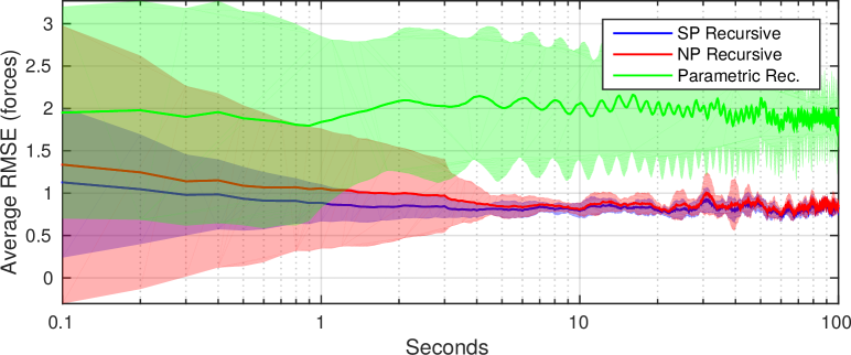
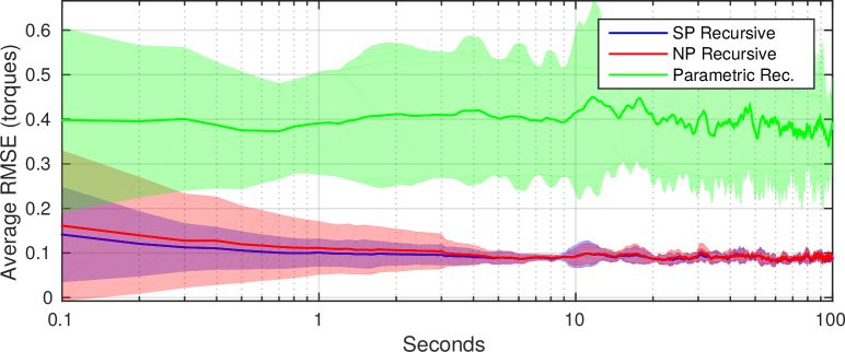
Figure 4: Predicted forces (top) and torques (bottom) components average RMSE, averaged over a 30-samples window for the recursive semiparametric (blue), nonparametric (red) and parametric (green) estimators. The solid lines indicate the mean values over 10 repetitions, and the transparent areas correspond to the standard deviations. On the $x$ axis, time (in seconds) is reported in logarithmic scale, in order to clearly show the behavior of the estimators during the initial transient phase. On the $y$ axis, the average RMSE is reported.

V CONCLUSIONS

We presented a novel incremental semiparametric modeling approach for inverse dynamics learning, joining together the advantages of parametric modeling derived from rigid body dynamics equations and of nonparametric Machine Learning methods. A distinctive trait of the proposed approach lies in its incremental nature, encompassing both the parametric and nonparametric parts and allowing for the prioritized update of both the identified base inertial parameters and the nonparametric weights. Such feature is key to enabling robotic systems to adapt to mutable conditions of the environment and of their own mechanical properties throughout extended periods. We validated our approach on the iCub humanoid robot, by analyzing the performances of a semiparametric inverse dynamics model of its right arm, comparing them with the ones obtained by state of the art fully nonparametric and parametric approaches.

References

- [1] R. Featherstone and D. E. Orin, “Dynamics.” in Springer Handbook of Robotics, B. Siciliano and O. Khatib, Eds. Springer, 2008, pp. 35–65.
- [2] A. E. Hoerl and R. W. Kennard, “Ridge Regression: Biased Estimation for Nonorthogonal Problems,” Technometrics, vol. 12, no. 1, pp. pp. 55–67, 1970.
- [3] C. Saunders, A. Gammerman, and V. Vovk, “Ridge Regression Learning Algorithm in Dual Variables.” in ICML, J. W. Shavlik, Ed. Morgan Kaufmann, 1998, pp. 515–521.
- [4] N. Cristianini and J. Shawe-Taylor, An Introduction to Support Vector Machines and Other Kernel-based Learning Methods. Cambridge University Press, 2000. [Online]. Available: https://books.google.it/books?id=B-Y88GdO1yYC
- [5] R. Rifkin, G. Yeo, and T. Poggio, “Regularized least-squares classification,” Nato Science Series Sub Series III Computer and Systems Sciences, no. 190, pp. 131–154, 2003.
- [6] C. E. Rasmussen and C. K. I. Williams, Gaussian Processes for Machine Learning. MIT Press, 2006. [Online]. Available: http://www.gaussianprocess.org/gpml;http://www.bibsonomy.org/bibtex/257ca77b8164cba5c6a0ac94918219119/3mta3
- [7] D. Nguyen-Tuong and J. Peters, “Using model knowledge for learning inverse dynamics.” in ICRA. IEEE, 2010, pp. 2677–2682.
- [8] A. Gijsberts and G. Metta, “Incremental learning of robot dynamics using random features.” in ICRA. IEEE, 2011, pp. 951–956.
- [9] T. Wu and J. Movellan, “Semi-parametric Gaussian process for robot system identification,” in Intelligent Robots and Systems (IROS), 2012 IEEE/RSJ International Conference on, Oct 2012, pp. 725–731.
- [10] J. Sun de la Cruz, D. Kulic, W. Owen, E. Calisgan, and E. Croft, “On-Line Dynamic Model Learning for Manipulator Control,” in IFAC Symposium on Robot Control, vol. 10, no. 1, 2012, pp. 869–874.
- [11] K. Yamane, “Practical kinematic and dynamic calibration methods for force-controlled humanoid robots.” in Humanoids. IEEE, 2011, pp. 269–275.
- [12] S. Traversaro, A. D. Prete, R. Muradore, L. Natale, and F. Nori, “Inertial parameter identification including friction and motor dynamics.” in Humanoids. IEEE, 2013, pp. 68–73.
- [13] Y. Ogawa, G. Venture, and C. Ott, “Dynamic parameters identification of a humanoid robot using joint torque sensors and/or contact forces.” in Humanoids. IEEE, 2014, pp. 457–462.
- [14] J. Hollerbach, W. Khalil, and M. Gautier, “Model identification,” in Springer Handbook of Robotics. Springer, 2008, pp. 321–344.
- [15] S. Vijayakumar and S. Schaal, “Locally Weighted Projection Regression: Incremental Real Time Learning in High Dimensional Space.” in ICML, P. Langley, Ed. Morgan Kaufmann, 2000, pp. 1079–1086.
- [16] B. Schölkopf and A. J. Smola, Learning with Kernels: Support Vector Machines, Regularization, Optimization, and Beyond (Adaptive Computation and Machine Learning). MIT Press, 2002.
- [17] A. Rahimi and B. Recht, “Random Features for Large-Scale Kernel Machines,” in NIPS. Curran Associates, Inc., 2007, pp. 1177–1184.
- [18] D. Nguyen-Tuong, M. Seeger, and J. Peters, “Model Learning with Local Gaussian Process Regression,” Advanced Robotics, vol. 23, no. 15, pp. 2015–2034, 2009. [Online]. Available: http://dx.doi.org/10.1163/016918609X12529286896877
- [19] G. Metta, L. Natale, F. Nori, G. Sandini, D. Vernon, L. Fadiga, C. von Hofsten, K. Rosander, M. Lopes, J. Santos-Victor, A. Bernardino, and L. Montesano, “The iCub Humanoid Robot: An Open-systems Platform for Research in Cognitive Development,” Neural Netw., vol. 23, no. 8-9, pp. 1125–1134, Oct. 2010.
- [20] M. Gautier and W. Khalil, “On the identification of the inertial parameters of robots,” in Decision and Control, 1988., Proceedings of the 27th IEEE Conference on. IEEE, 1988, pp. 2264–2269.
- [21] M. Gautier, “Dynamic identification of robots with power model,” in Robotics and Automation, 1997. Proceedings., 1997 IEEE International Conference on, vol. 3. IEEE, 1997, pp. 1922–1927.
- [22] K. Ayusawa, G. Venture, and Y. Nakamura, “Identifiability and identification of inertial parameters using the underactuated base-link dynamics for legged multibody systems,” The International Journal of Robotics Research, vol. 33, no. 3, pp. 446–468, 2014.
- [23] J. Baelemans, P. van Zutven, and H. Nijmeijer, “Model parameter estimation of humanoid robots using static contact force measurements,” in Safety, Security, and Rescue Robotics (SSRR), 2013 IEEE International Symposium on, Oct 2013, pp. 1–6.
- [24] W. Khalil and E. Dombre, Modeling, identification and control of robots. Butterworth-Heinemann, 2004.
- [25] A. Rahimi and B. Recht, “Uniform approximation of functions with random bases,” in Communication, Control, and Computing, 2008 46th Annual Allerton Conference on, Sept 2008, pp. 555–561.
- [26] W. Rudin, Fourier Analysis on Groups, ser. A Wiley-interscience publication. Wiley, 1990.
- [27] Å. Björck, Numerical Methods for Least Squares Problems. Siam Philadelphia, 1996.
- [28] A. H. Sayed, Adaptive Filters. Wiley-IEEE Press, 2008.
- [29] A. Tacchetti, P. K. Mallapragada, M. Santoro, and L. Rosasco, “GURLS: a least squares library for supervised learning,” The Journal of Machine Learning Research, vol. 14, no. 1, pp. 3201–3205, 2013.
- [30] D. M. Beazley et al., “SWIG: An easy to use tool for integrating scripting languages with C and C++,” in Proceedings of the 4th USENIX Tcl/Tk workshop, 1996, pp. 129–139.
- [31] S. Traversaro, A. Del Prete, S. Ivaldi, and F. Nori, “Inertial parameters identification and joint torques estimation with proximal force/torque sensing,” in 2015 IEEE International Conference on Robotics and Automation (ICRA 2015).
- [32] S. Ivaldi, M. Fumagalli, M. Randazzo, F. Nori, G. Metta, and G. Sandini, “Computing robot internal/external wrenches by means of inertial, tactile and F/T sensors: Theory and implementation on the iCub,” in Humanoid Robots (Humanoids), 2011 11th IEEE-RAS International Conference on, Oct 2011, pp. 521–528.
- [33] U. Pattacini, F. Nori, L. Natale, G. Metta, and G. Sandini, “An experimental evaluation of a novel minimum-jerk cartesian controller for humanoid robots,” in Intelligent Robots and Systems (IROS), 2010 IEEE/RSJ International Conference on, Oct 2010, pp. 1668–1674.