Tailored pump-probe transient spectroscopy with time-dependent density-functional theory: controlling absorption spectra

Abstract

Recent advances in laser technology allow us to follow electronic motion at its natural time-scale with ultra-fast time resolution, leading the way towards attosecond physics experiments of extreme precision. In this work, we assess the use of tailored pumps in order to enhance (or reduce) some given features of the probe absorption (for example, absorption in the visible range of otherwise transparent samples). This type of manipulation of the system response could be helpful for its full characterization, since it would allow to visualize transitions that are dark when using unshaped pulses. In order to investigate these possibilities, we perform first a theoretical analysis of the non-equilibrium response function in this context, aided by one simple numerical model of the Hydrogen atom. Then, we proceed to investigate the feasibility of using time-dependent density-functional theory as a means to implement, theoretically, this absorption-optimization idea, for more complex atoms or molecules. We conclude that the proposed idea could in principle be brought to the laboratory: tailored pump pulses can excite systems into light-absorbing states. However, we also highlight the severe numerical and theoretical difficulties posed by the problem: large-scale non-equilibrium quantum dynamics are cumbersome, even with TDDFT, and the shortcomings of state-of-the-art TDDFT functionals may still be serious for these out-of-equilibrium situations.

I Introduction

Time-resolved pump-probe experiments are powerful techniques to study the dynamics of atoms and molecules: the pump pulse triggers the dynamics, which is then monitored by measuring the time-dependent response of the excited system to a probe pulse. The time-resolution of this technique has increased over the years, and nowadays, it can be used to observe the electron dynamics in real time, giving rise to the field of attosecond physics Krausz and Ivanov (2009); Scrinzi et al. (2006).

A suitable setup to observe charge-neutral excitations is the time-resolved photoabsorption or transient absorption spectroscopy (TAS), where the time-dependent optical absorption of the probe is measured. TAS can of course be used to look at longer time resolutions: if we look at molecular reaction on the scale of tens or hundreds of femtoseconds, the atomic structure will have time to re-arrange. These techniques are thus mainly employed in femtochemistry Zewail (1994, 2000) to observe and control modification, creation, or destruction of bonds. TAS has been successfully employed, for example, to watch the first photo-synthetic events in cholorophylls and carotenoids Berera et al. (2009) (a review describing the essentials of this technique can be found in Ref. Foggi et al. (2001)). If, on the contrary, one wants to study the electronic dynamics only, disentangling it from the vibronic degrees of freedom, then one must perform TAS with attosecond pulses Pfeifer et al. (2008), a possibility recently demonstrated Goulielmakis et al. (2010); Holler et al. (2011).

The theoretical description of these processes, which involve non-linear light-matter interaction, and the ensuing non-equilibrium electron dynamics, is challenging. Time-dependent density functional theory (TDDFT) Runge and Gross (1984); Marques et al. (2011); tdd is a well-established tool to compute the response of a many-electron system to arbitrary perturbations. Traditionally, the vast majority of TDDFT applications have addressed the first-order response of the ground-state system to weak electric fields – which can provide the absorption spectrum, the optically-allowed excitation energies and oscillator strengths, etc. Nevertheless, the extension of TDDFT to the description of excited state spectral properties and its ability to simulate transient absorption spectroscopy (TAS) has recently been demonstrated De Giovannini et al. (2012, 2013).

In this work, we are not only interested in simulating attosecond TAS of atoms and molecules, but in studying the possibility of tailoring the pump to control the spectra. In fact, the measurement and control of ultrafast processes are inherently intertwined: quantum optimal control theory (QOCT) Brif et al. (2010); Werschnik and Gross (2007) can be viewed as the inverse of theoretical spectroscopy: rather than attempting to predict the reaction of a quantum system to a perturbation, it attempts to find the perturbation that induces a given reaction in a given quantum system. It is the quantum version of the more general control theory Shi et al. (1988); Peirce et al. (1988); Kosloff et al. (1989); Luenberger (1969, 1979), which was needed given the fast advances in experimental quantum control Brumer and Shapiro (1986a, b); Shapiro and Brumer (2003); Tannor and Rice (1985); Herek et al. (1994); Gaubatz et al. (1988); Ohmori (2009); Judson and Rabitz (1992); Bardeen et al. (1997); Assion et al. (1998).

The possibility of combining QOCT with TDDFT has been established recently Castro et al. (2012). Furthermore it has been shown, that it can be used to optimize strong-field ionization Hellgren et al. (2013), photo-induced dissociation Castro (2013) and is compatible with Ehrenfest dynamics Castro and Gross (2014). Very recently, Krieger et al. used TDDFT to study the influence of laser intensity, frequency and duration on the laser-induced demagnetization process in bulk materials, which takes place on time scales of $<$ 20 fs Krieger et al. .

Here, we take the first steps towards the use of this combination of TDDFT with QOCT to control excited state spectra of finite systems. This idea is very much related to the concept of electromagnetically induced transparency Harris et al. (1990); Fleischhauer et al. (2005). Control of the absorption spectra may mean its elimination or reduction, or its increase. Our gedanken setup throughout this paper is the following: for a certain time interval $[0,T]$ a quantum system is driven by a “classical” pump pulse $\mathscr{E}(t)$ whose precise shape can be manipulated. After the pump has ended, the (linear) response of the system to some later perturbation is calculated. Our goal is to design the shape of the pump pulse in such a way, that the response to some later perturbation is optimal in some given way. In particular, we demonstrate how the tailored pump pulses may be used to transform a transparent atom or molecule into an excited one that absorbs in the visible.

This paper is structured as follows. In Section II, we analyze the optical linear response of a system in an excited state, looking at the location and the shape of the resulting spectral peaks and their time-dependence. In Section III we present the theory of quantum optimal control and how it can be applied to optimize spectral properties of systems in excited states. We then bring these concepts into application in Section IV. In Section IV.1 we illustrate the conclusions gained in Section II using the analyticly solvable Hydrogen atom. We then proceed to demonstrate control of the excited state properties in this system. In Section IV.2 we finally combine our methodology with time-dependent density functional theory, first for the Helium atom, and then for the Methane molecule. We conclude our work in Section V.

II Short Review of Out-of-equilibrium (Pumped) Absorption Spectra

In pump-probe spectroscopy, the probe may arrive after, during, or even before the pump; in this work, we consider a non-overlapping regime in which the probe arrives after the pump has vanished. The time evolution of a system after the end of the pump is described by the Hamiltonian (atomic units will be used hereafter):

$$\hat{H}(t)=\mathscr{\hat{H}}+F(t)\hat{D}_{\mu}\,,$$ (1)

where $\mathscr{\hat{H}}$ is the static Hamiltonian, that describes the system itself and $F(t)\hat{D}_{\mu}$ is the coupling to a probe pulse via the dipole operator

$$\hat{D}_{\mu}=-\sum_{i=1}^{N}\hat{r}_{\mu}^{(i)}$$ (2)

in which $N$ is the number of electrons in the system, and $\mu=x,y,z$ determines the polarization direction. Note, that the implementation of the coupling via the dipole operator is an approximation and could be removed in practical implementations since the theory handles non-dipolar fields. Also note, that we work in the length gauge all over the paper.

If, at the time $t=T$, the system has been driven by the previous pump $\mathscr{E}$ to the state $|\Psi\left[\mathscr{E}\right](T)\rangle$, the complete dipole-dipole response function for the perturbation at later times is given by:

$$\chi_{\hat{D}_{\mu},\hat{D}_{\nu}} \left[\mathscr{E}\right](t,t^{\prime})=$$

$$-i\theta(t-t^{\prime})\langle\Psi\left[\mathscr{E}\right](T)|\left[\hat{D}_{\mu I}(t),\hat{D}_{\nu I}(t^{\prime})\right]|\Psi\left[\mathscr{E}\right](T)\rangle\,,$$

where the operators are expressed in the interaction picture.

The difference between Eq. (II) and the equilibrium response function Alexander L. Fetter (2003) or the response function of a system in a many-body eigenstate is that the two times $t$ and $t^{\prime}$ cannot be reduced to only one by making use of the time-translational invariance. Since $|\Psi\left[\mathscr{E}\right](T)\rangle$ depends on the pump, the first-order response of the system does explicitly depend on both the pump $\mathscr{E}$ and the probe $F$. It is given by:

$$D^{(1)}_{\mu\nu}\left[\mathscr{E},F\right](t)=\int_{T}^{t}\!{\rm d}t^{\prime}F(t^{\prime})\chi_{\hat{D}_{\mu},\hat{D}_{\nu}}\left[\mathscr{E}\right](t,t^{\prime})\,.$$ (4)

An intuitive physical meaning can be gained from this equation for the response function: it is the first order of the system response, if we consider a sudden perturbation at $t^{\prime}=T+\tau\mathrel{\mathop{\mathchar 58\relax}}F(t)=\delta(t-(T+\tau))$, where $\tau$ denotes the delay between the end of the pump and the perturbation:

$$\chi_{\hat{D}_{\mu},\hat{D}_{\nu}}\left[\mathscr{E}\right](t,T+\tau)=D^{(1)}_{\mu\nu}\left[\mathscr{E},\delta_{T+\tau}\right](t)\,.$$ (5)

This object contains all the necessary information about the interacting system to compute the absorption of any given probe, as long as it is weak enough for the response to be linear. In order to analyze it, it is useful to take the Fourier transform with respect to the variable $t$, and expand Eq. (II) in an eigenbasis of the static Hamiltonian $\mathscr{\hat{H}}$

$$|\Psi\left[\mathscr{E}\right](T)\rangle=\operatorname*{\mathchoice{\ooalign{$\displaystyle\sum$\cr$\displaystyle\int$\cr}}{\ooalign{\raisebox{0.14pt}{\scalebox{0.7}{$\textstyle\sum$}}\cr$\textstyle\int$\cr}}{\ooalign{\raisebox{0.2pt}{\scalebox{0.6}{$\scriptstyle\sum$}}\cr$\scriptstyle\int$\cr}}{\ooalign{\raisebox{0.2pt}{\scalebox{0.6}{$\scriptstyle\sum$}}\cr$\scriptstyle\int$\cr}}}_{j=1}^{\infty}\gamma_{j}|\Phi_{j}\rangle,\qquad\mathscr{\hat{H}}|\Phi_{j}\rangle=\varepsilon_{j}|\Phi_{j}\rangle\,,$$ (6)

obtaining a Lehmann representation for the time-dependent non-equilibrium response function:

$$\chi_{\hat{D}_{\mu},\hat{D}_{\nu}} \left[\mathscr{E}\right](\omega,T+\tau)=$$ (16)

$$\operatorname*{\mathchoice{\ooalign{$\displaystyle\sum$\cr$\displaystyle\int$\cr}}{\ooalign{\raisebox{0.14pt}{\scalebox{0.7}{$\textstyle\sum$}}\cr$\textstyle\int$\cr}}{\ooalign{\raisebox{0.2pt}{\scalebox{0.6}{$\scriptstyle\sum$}}\cr$\scriptstyle\int$\cr}}{\ooalign{\raisebox{0.2pt}{\scalebox{0.6}{$\scriptstyle\sum$}}\cr$\scriptstyle\int$\cr}}}_{jkm}d^{\mu}_{jm}d^{\nu}_{mk}\left\{\frac{\gamma_{j}\gamma_{k}^{*}e^{i\omega_{jk}\tau}}{\omega+\omega_{jm}+i\nicefrac{{\Gamma}}{{2}}}-\frac{\gamma_{j}^{*}\gamma_{k}e^{-i\omega_{jk}\tau}}{\omega-\omega_{jm}+i\nicefrac{{\Gamma}}{{2}}}\right\}$$

in terms of the exact energy differences $\omega_{jk}=\varepsilon_{k}-\varepsilon_{j}$, the dipole-matrix elements $d^{\mu}_{jm}=\langle\Phi_{j}|\hat{D}_{\mu}|\Phi_{m}\rangle\in\mathbb{R}$ and the pump-probe delay $\tau$. A similar representation in the case of non-equilibrium spectroscopy has been recently presented in a similar context Perfetto and Stefanucci (2015). By writing $\gamma_{j}=|\gamma_{j}|e^{i\varphi_{j}}$ Eq. (16) turns into

$$\chi_{\hat{D}_{\mu},\hat{D}_{\nu}}\left[\mathscr{E}\right](\omega,T+\tau)=$$ (17)

$$\operatorname*{\mathchoice{\ooalign{$\displaystyle\sum$\cr$\displaystyle\int$\cr}}{\ooalign{\raisebox{0.14pt}{\scalebox{0.7}{$\textstyle\sum$}}\cr$\textstyle\int$\cr}}{\ooalign{\raisebox{0.2pt}{\scalebox{0.6}{$\scriptstyle\sum$}}\cr$\scriptstyle\int$\cr}}{\ooalign{\raisebox{0.2pt}{\scalebox{0.6}{$\scriptstyle\sum$}}\cr$\scriptstyle\int$\cr}}}_{jkm}d^{\mu}_{jm}d^{\nu}_{mk}|\gamma_{j}\gamma_{k}|\left\{\frac{e^{i\Theta_{kj}(\tau)}}{\omega+\omega_{jm}+i\nicefrac{{\Gamma}}{{2}}}-\frac{e^{-i\Theta_{kj}(\tau)}}{\omega-\omega_{jm}+i\nicefrac{{\Gamma}}{{2}}}\right\}$$ (26)

with

$$\Theta_{kj}(\tau)=\varphi_{j}-\varphi_{k}-\omega_{kj}\tau\,.$$ (27)

Since the absorption depends on the imaginary part of the response function, we get from Eq. (17):

$$\Im\chi_{\hat{D}_{\mu},\hat{D}_{\nu}}\left[\mathscr{E}\right](\omega,T+\tau)=\operatorname*{\mathchoice{\ooalign{$\displaystyle\sum$\cr$\displaystyle\int$\cr}}{\ooalign{\raisebox{0.14pt}{\scalebox{0.7}{$\textstyle\sum$}}\cr$\textstyle\int$\cr}}{\ooalign{\raisebox{0.2pt}{\scalebox{0.6}{$\scriptstyle\sum$}}\cr$\scriptstyle\int$\cr}}{\ooalign{\raisebox{0.2pt}{\scalebox{0.6}{$\scriptstyle\sum$}}\cr$\scriptstyle\int$\cr}}}_{jkm}d^{\mu}_{jm}d^{\nu}_{mk}|\gamma_{j}\gamma_{k}|$$ (36)

$$\left\{\cos(\Theta_{kj}(\tau))L(\omega-\omega_{jm})+\sin(\Theta_{kj}(\tau))R(\omega-\omega_{jm})\right.$$

$$\left.-\cos(\Theta_{kj}(\tau))L(\omega+\omega_{jm})+\sin(\Theta_{kj}(\tau))R(\omega+\omega_{jm})\right\}$$

with the Rayleigh peaks

$$R(\bar{\omega})=\frac{\bar{\omega}}{\bar{\omega}^{2}+\nicefrac{{\Gamma^{2}}}{{4}}}$$ (38)

and the Lorentzian peaks

$$L(\bar{\omega})=\frac{\nicefrac{{\Gamma}}{{2}}}{\bar{\omega}^{2}+\nicefrac{{\Gamma^{2}}}{{4}}}\,.$$ (39)

The absorption cross section tensor is:

$$\sigma_{\mu,\nu}(\omega)=\frac{4\pi\omega}{c}\Im\chi_{\hat{D}_{\mu}\hat{D}_{\nu}}(\omega)\,,$$ (40)

and for a random sample, the absorption will be its orientational average, i.e. the absorption coefficient:

$$\bar{\sigma}(\omega)=\frac{1}{3}\operatorname{Tr}\sigma(\omega)\,.$$ (41)

Since we are only interested in the trace, in the following, we concentrate on the diagonal terms, we will omit hereafter the orientation indexes in order to ease the notation.

We now analyze Eq. (LABEL:eq:chi_final) in more detail. First, as already pointed out in Ref. Perfetto and Stefanucci (2015), in this non-overlapping regime the dependence of the spectrum on both the pump-pulse and the delay time enters through the modification of the peak amplitudes and shapes exclusively: the peak positions are intrinsic properties of the many-body system. Second, for the analysis of the effect of the pump pulse and of the pump-probe delay on the spectrum, we can distinguish between three cases: (i) the system is in its ground state, (ii) the system is in an excited eigenstate, (iii) the system is in a non-stationary state, i.e. in a linear combination of non-degenerate eigenstates. In all cases we focus on the positive part of the energy range, which we denote by $\omega^{+}$. The following shape analysis in terms of Lorentzian and Rayleigh contributions is for discrete peaks only. We denote this by replacing $\operatorname*{\mathchoice{\ooalign{$\displaystyle\sum$\cr$\displaystyle\int$\cr}}{\ooalign{\raisebox{0.14pt}{\scalebox{0.7}{$\textstyle\sum$}}\cr$\textstyle\int$\cr}}{\ooalign{\raisebox{0.2pt}{\scalebox{0.6}{$\scriptstyle\sum$}}\cr$\scriptstyle\int$\cr}}{\ooalign{\raisebox{0.2pt}{\scalebox{0.6}{$\scriptstyle\sum$}}\cr$\scriptstyle\int$\cr}}}$ by $\sum$ (we will comment on the continuum part later on in this section).

In case (i) $\gamma_{i}=\delta_{i0}$ and $\Im\chi_{\hat{D},\hat{D}}\left[\mathscr{E}\right](\omega^{+})$ reduces to the usual Lehmann representation for the ground state spectrum:

$$\Im\chi_{\hat{D},\hat{D}}\left[\mathscr{E}\right](\omega^{+})=\sum_{m}|d_{0m}|^{2}L(\omega^{+}-\omega_{0m}).$$ (42)

All peaks are positive and have Lorentzian shape. In case (ii), where $\gamma_{i}=\delta_{i\xi}$, the system is in an excited eigenstate $\Phi_{\xi}$, and therefore in the positive energy part of the spectrum we can find both positive and negative peaks of Lorentzian shape:

$$\Im\chi_{\hat{D},\hat{D}} \left[\mathscr{E}\right](\omega^{+})=$$

$$\sum_{\xi<m}|d_{\xi m}|^{2}L(\omega^{+}-\omega_{\xi m})-\sum_{\xi>m}|d_{\xi m}|^{2}L(\omega^{+}+\omega_{\xi m})\,.$$

Note, that in both cases (i) and (ii), the spectrum is time-independent and has only Lorentzian contributions. This is the main difference to the case (iii), for non-stationary states. In this case, the spectrum can be divided into two parts, one time-independent and one oscillatory part due to interferences between the involved states:

$$\Im\chi_{\hat{D},\hat{D}} \left[\mathscr{E}\right](\omega^{+},T+\tau)=$$

$$\Im\chi_{\hat{D},\hat{D}}^{0}\left[\mathscr{E}\right](\omega^{+})+\Im\chi_{\hat{D},\hat{D}}^{\rm INT}\left[\mathscr{E}\right](\omega^{+},T+\tau)$$

The equilibrium term consists of the sum over the stationary state spectra of the eigenstates involved, scaled by their occupations:

$$\Im \chi_{\hat{D},\hat{D}}^{0}\left[\mathscr{E}\right](\omega^{+})=\sum_{j}|\gamma_{j}|^{2}\times$$

$$\left\{\sum_{j<m}|d_{jm}|^{2}L(\omega-\omega_{jm})-\sum_{j>m}|d_{jm}|^{2}L(\omega+\omega_{jm})\right\}\,.$$

Its peaks are always of Lorentzian shape and depend neither on time nor on the initial phase difference $\varphi_{j}-\varphi_{k}$. It is influenced by the pump laser only through the occupations $|\gamma_{j}|^{2}$. The phase- and time-dependency of the spectrum enters through the interference term

$$\Im\chi_{\hat{D},\hat{D}}^{\rm INT}\left[\mathscr{E}\right](\omega,T+\tau)=\sum_{j\neq k;m}d_{jm}d_{mk}|\gamma_{j}\gamma_{k}|\left\{\right.$$

$$\cos\Theta_{kj}(\tau)L(\omega-\omega_{jm})+\sin\Theta_{kj}(\tau)R(\omega-\omega_{jm})$$

$$- \left.\cos\Theta_{kj}(\tau)L(\omega+\omega_{jm})+\sin\Theta_{kj}(\tau)R(\omega+\omega_{jm})\right\}$$

which in turn is governed by the phase differences $\Theta_{kj}$, which have contributions from both the phase difference $\varphi_{j}-\varphi_{k}$ at the end of the laser and from its time evolution $\omega_{kj}\tau$. $\Theta_{kj}$ mixes real and imaginary part of the response function and converts Lorentzian line shapes into Rayleigh line shapes and vice versa. This conversion happens periodically with the frequency given by the energy differences $\omega_{kj}$ between the occupied states involved. The time-dependence of a spectrum is therefore a clear sign of a non-stationary state. Experimentally, this periodic beating pattern was recently observed by Goulielmakis et al Goulielmakis et al. (2010). This demonstrates, how using a pump to imprint an internal phase difference $\varphi_{j}-\varphi_{k}$ onto a state and controlling the delay time $\tau$ between pump and probe laser can be used to change a spectrum, converting absorption into emission peaks (and vice versa) as well as changing the overall shape of the lines. In Section IV.1 we demonstrate these line shape changes using the example of an exactly solvable Hydrogen atom. Furthermore we demonstrate, how to use a laser to control these features.

Note, that in the discussion above, the lineshape analysis is valid for isolated peaks without contribution from continuum states. If coupling to continuum states is involved, an additional shaping comes from the dependence of the matrix elements $d_{jm}$ on the energy. This is e.g. the case for Fano line-shapes which may acquire a complex Fano $q$ factor Zielinski et al. (2014).

III Quantum Optimal Control of Excited State Spectra

In this work we employ Quantum Optimal Control Theory (QOCT) to optimize the response of a system in the situation described in the previous section. QOCT is concerned with studying the optimal Hamiltonian (in practice, a portion of the Hamiltonian, such as the temporal profile of the coupling of an atom or molecule to a laser pulse) that induces a target system behaviour. In the following, we present its specific application to the problem of optimizing response functions of excited states. We will also show how, if the problem can be reduced to a small model, it can be solved analytically.

Let us consider a quantum mechanical system governed by the Schrödinger equation during the time interval [0,T]:

$$i\frac{\partial\Psi}{\partial t}(x,t) = \hat{H}[\mathscr{E},t]\Psi(x,t)\,,$$ (47a)

$$\Psi(x,0) = \Psi_{0}(x)\,,$$ (47b)

where $x$ is the full set of quantum coordinates, and $\mathscr{E}$ is the control field, an external potential applied to the system (in our case, the pump pulse). In order to perform optimizations the field must be discretized, for example with the help of a sine Fourier basis. In our numerical simulations:

$$\mathscr{E}_{\mathbf{c}}(t)=\sum_{n=1}^{M}c_{n}\sin(\omega_{n}t)$$ (48)

where $M$ is the dimension of the optimization search space, and $\mathbf{c}$ is the set of all the parameters that determine the field: $\mathbf{c}=c_{1},\dots,c_{M}$. The frequencies, and their maximum value or cut-off frequency, may be chosen at will.

The specification of $\mathscr{E}$, together with an initial value condition, $\Psi(0)=\Psi_{0}$ determines the full evolution of the system, $\Psi[\mathscr{E}]$, via the propagation of the Schrödinger equation. The behaviour of the system must then be measured by defining a “target functional” $F$, whose value is high if the system evolves according to our goal, and small otherwise. In many cases, it is split into two parts, $F[\Psi,\mathscr{E}]=J_{1}[\Psi]+J_{2}[\mathscr{E}]$, so that $J_{1}$ only depends on the state of the system, and $J_{2}$, called the “penalty”, depends explicitly on the control $\mathscr{E}$. Regarding $J_{1}$, it may depend on the full evolution of the system during the time interval $[0,T]$, or only on the system state at time $T$, as it is the case in this work. Often, the functional is defined through the expectation value of an observable $\hat{O}$:

$$J_{1}^{T}[\Psi(T)]=\langle\Psi(T)|\hat{O}|\Psi(T)\rangle\,.$$ (49)

The mathematical problem is then reduced to the problem of maximizing a real-valued function $G$:

$$G[\mathbf{c}]=F[\Psi[\mathscr{E}_{\mathbf{c}}],\mathscr{E}_{\mathbf{c}}]\,.$$ (50)

The absorption of light is related to the average absorption coefficient $\bar{\sigma}[\mathscr{E}\mathbf{c}](E)$ [Eq. (41)]. The larger the absorption coefficient at a certain energy, the more light is absorbed at this energy. In order to find a laser pulse to make a system, that is transparent in its ground state, absorb as much light as possible, we therefore optimize the absorption coefficient in the visible by taking the integral of $\bar{\sigma}[\mathscr{E}_{\mathbf{c}}](E)$ over the respective energy range. We employed two different control targets:

$$G_{\tau}^{A}\left[\mathbf{c}\right] = \int_{E_{min}}^{E_{max}}\!\!\!\!dE\,\,\bar{\sigma}_{\tau}[\mathscr{E}_{\mathbf{c}}](E)\,,$$ (51a)

$$G_{\tau}^{B}\left[\mathbf{c}\right] = \int_{E_{min}}^{E_{max}}\!\!\!\!dE\,\,\bar{\sigma}_{\tau}[\mathscr{E}_{\mathbf{c}}](E)e^{\left(-\gamma\frac{N_{0}-N_{T}[\mathscr{E}]}{N_{0}}\right)}\,,$$ (51b)

where $\bar{\sigma}_{\tau}[\mathscr{E}_{\mathbf{c}}](E)$ [in the following we will call it just $\bar{\sigma}(E)$] is the average absorption coefficient of the system at a given time delay $\tau$ after the pump pulse $\mathscr{E}(t)$, and $E_{min}$ and $E_{max}$ define the optimization region - the energy range, where the absorption is optimized. In the second target function we have introduced an exponential factor that depends on $N_{0}$ and $N_{T}$, the number of electrons in the system at the beginning and the end of the pump pulse, respectively. The reason to introduce this factor is to avoid ionization, i.e. we wish to lead the system to a state with the desired absorption properties, but keeping the ionization probability low. Keeping the ionization low is particularly important in the TDDFT calculations, if performed with adiabatic functionals, since with current state-of-the-art adiabatic functionals, ionization of the system leads to unphysical shifts in the position of the absorption peaks. The term $\exp{\left(-\gamma\frac{N_{0}-N_{T}[\mathscr{E}]}{N_{0}}\right)}$ therefore inflicts a penalty, whose strength can be modulated by $\gamma$, to pump pulses that produce strong ionization. We implement ionization using absorbing boundaries and thus the total number of electrons is, in general, not conserved during time. In practice, one can also combine the two target functions: one may start optimizations using $G_{\tau}^{A}$, and later continue with $G_{\tau}^{B}$, restarting from the previous optimum.

Once the target is defined one is left with the problem of choosing an optimization algorithm to find the maximum (or maxima) of $G$. Two broad families can be distinguished: gradient-free procedures, which only require the computation of $G$ given a control input $\mathscr{E}$, and gradient-based procedures, that also require the computation of the gradient of $G$ with respect to $\mathscr{E}$. QOCT provides an expression for the gradient that can be adapted for this case (see appendix A for details). This approach, however is numerically unfeasible for the target covered in this paper. For this reason, in our simulations, we employed the gradient-free Simplex-Downhill algorithm by Nelder and Mead Nelder and Mead (1965).

In principle, if the system can be reduced to a few-level model, the optimal fields can be found analytically. To illustrate this approach, below we briefly illustrate a simple example of controlling the absorption properties of a single Hydrogen atom. Instead of directly optimizing $G_{\tau}^{A,B}$ we here derive a laser that drives the system into a state with the wanted optical properties. Let us suppose that the situation can be approximated by a three-level Hamiltonian $\mathscr{\hat{H}}$ with eigenstates $|\Phi_{a}\rangle$, $|\Phi_{b}\rangle$ and $|\Phi_{c}\rangle$ and the corresponding eigenenergies $\varepsilon_{a}$, $\varepsilon_{b}$ and $\varepsilon_{c}$. We define the transition energies $\omega_{ab}=\varepsilon_{b}-\varepsilon_{a}$, $\omega_{bc}=\varepsilon_{c}-\varepsilon_{b}$ and $\omega_{ac}=\varepsilon_{c}-\varepsilon_{a}$. The dipole coupling between the states is given by $d_{ab}$ and $d_{ac}$ (both assumed to be real numbers), and we further consider the case where the coupling between the states $|\Phi_{b}\rangle$ and $|\Phi_{c}\rangle$ is dipole forbidden.

The system is pumped by a laser field composed of two carrier frequencies $\omega_{1,2}$ of the form:

$$\mathscr{E}(t)=\tilde{\varepsilon}_{1}(t)\cos(\omega_{1}t+\varphi_{1})+\tilde{\varepsilon}_{2}(t)\cos(\omega_{2}t+\varphi_{2}),$$ (52)

with phases $\varphi_{1,2}$, amplitudes $\varepsilon_{1,2}$ and envelope $\tilde{\varepsilon}_{1,2}(t)$ defined by

$$\tilde{\varepsilon}_{1,2}(t) = 2\varepsilon_{1,2}\sin^{2}\left(\pi\frac{t}{T}\right)\,.$$ (53)

Our goal is to find a laser pulse that drives the system from state $|\Psi(t=0)\rangle=|\Phi_{a}\rangle$ into a target state $|\bar{\Psi}\rangle$

$$|\bar{\Psi}\rangle=\alpha|\Phi_{a}\rangle+\beta|\Phi_{b}\rangle+\gamma|\Phi_{c}\rangle$$ (54)

in a given time $T$ – $\alpha,\beta,$ and $\gamma$ are complex coefficients. Since the spectral properties of this state can be then easily obtained using Eqs. (II), (41), the problem of finding a pulse giving the desired optical properties translates to the one of maximizing the overlap $|\langle\Psi(T)|\bar{\Psi}\rangle|^{2}$ while keeping the functional form of the laser fixed – i.e. changing only $\omega_{1,2}$, $\varphi_{1,2}$, and $\varepsilon_{1,2}$. If we choose $\omega_{1,2}$ resonant with the transition frequencies $\omega_{ab},\omega_{ac}$ and assume they are sufficiently separated in energy we can apply the rotating wave approximation and obtain the laser parameters as function of $\alpha,\beta,\gamma$ as (see Appendix B for details):

$$\varepsilon_{1} = \frac{2}{T}\frac{\arccos(|\alpha|)}{\sin(\arccos(|\alpha|)}\frac{|\beta|}{d_{ab}}$$ (55a)

$$\varepsilon_{2} = \frac{2}{T}\frac{\arccos(|\alpha|)}{\sin(\arccos(|\alpha|)}\frac{|\gamma|}{d_{ac}}$$ (55b)

and

$$\varphi_{\beta} = \varphi_{1}-\pi+\omega_{ba}T$$ (55c)

$$\varphi_{\gamma} = \varphi_{2}-\pi+\omega_{ca}T\,.$$ (55d)

We will come back to this example below in Sec. IV.1.

IV Applications

Any QOCT formulation is constructed on top of a given model for the physics of the process under study. In this paper we study and optimize the absorption spectra of atoms and molecules using either analytically solvable model Hamiltonians or obtaining the spectra by using time-dependent density functional theory (TDDFT) Marques et al. (2011); tdd – the time-dependent counterpart of DFT Kohn (1999).

Based on the Runge-Gross theorem Runge and Gross (1984) TDDFT establishes a one-to-one correspondence between the time-dependent density and the time-dependent external potential of a many-electron system. Together with the Kohn-Sham (KS) scheme Kohn and Sham (1965) it allows us to recast the many-body time-dependent problem into a simpler one where the interacting electrons are replaced by a fictitious set of non-interacting electrons with the same time-dependent density. This system of non-interacting electrons can then be represented with a single Slater determinant formed by a set of KS orbitals leading to great computational simplifications.

In the following we will work with spin-compensated systems of $N$ electrons doubly occupying $N/2$ spatial orbitals. The time evolution of these orbitals $\varphi_{i}$ ($i=1,N/2$), is governed by the time-dependent Kohn-Sham equations

$${\rm i}\frac{\partial}{\partial t}\varphi_{i}({\mathbf{r}},t) = -\frac{1}{2}\nabla^{2}\varphi_{i}({\mathbf{r}},t)+v_{\rm KS}[n]({\mathbf{r}},t)\varphi_{i}({\mathbf{r}},t)\,,$$ (56)

$$n({\mathbf{r}},t) = 2\sum_{i=1}^{N/2}|\varphi_{i}({\mathbf{r}},t)|^{2}\,,$$ (57)

where $v_{\rm KS}[n]({\mathbf{r}},t)$ is the KS potential. It is, in general, a functional of the density and is defined as

$$v_{\rm KS}[n]({\mathbf{r}},t)=v_{0}({\mathbf{r}})+v({\mathbf{r}},t)+v_{\rm H}[n]({\mathbf{r}},t)+v_{\rm xc}[n]({\mathbf{r}},t)\,,$$ (58)

where $v_{0}({\mathbf{r}})$ represents the static (ionic) external potential, $v({\mathbf{r}},t)=\mathcal{E}(t)\cdot{{\mathbf{r}}}$ is the coupling to the time dependent electric field $\mathcal{E}(t)$ in the dipole approximation (in the length gauge), $v_{\rm H}[n]({\mathbf{r}},t)=\int\!{\rm d}^{3}r^{\prime}\,n({\mathbf{r}},t)/|{\mathbf{r}}^{\prime}-{\mathbf{r}}|$ is the classical electrostatic Hartree potential, and $v_{\rm xc}[n]({\mathbf{r}},t)$ is the exchange and correlation potential accounting for the many electron effects Marques et al. (2011, 2012). In our simulations the ions are clamped to their equilibrium positions. All numerical calculations were performed using the octopus code Marques et al. (2003).

IV.1 One Electron Systems: the Hydrogen Atom

In Section II we have discussed how the amplitudes and shapes of excited state absorption spectra depend on the relative phases $\varphi_{i}$ of the expansion coefficients $\gamma_{i}$. Here, we illustrate this effect in a Hydrogen atom, which is initially pumped into the state

$$|\bar{\Psi}\rangle=\sqrt{0.4}|2p_{z}\rangle+\sqrt{0.6}e^{i\varphi}|3p_{z}\rangle\,.$$ (59)

Let us first vary $\varphi$ to show the effect of the phase on the final spectrum. For our pumped state the stationary part of the spectrum is composed of the weighted stationary state spectra coming from $|2p_{z}\rangle$ and $|3p_{z}\rangle$:

$$\bar{\sigma}^{0}(\omega)=0.4\bar{\sigma}_{2p_{z}}(\omega)+0.6\bar{\sigma}_{3p_{z}}(\omega)\,,$$ (60)

whereas the phase-dependent interference term is

$$\bar{\sigma}^{\rm INT}(\omega,\varphi)=0.4\cdot 0.6\cdot\frac{4\pi\omega}{3c}\;\Big{[}\operatorname*{\mathchoice{\ooalign{$\displaystyle\sum$\cr$\displaystyle\int$\cr}}{\ooalign{\raisebox{0.14pt}{\scalebox{0.7}{$\textstyle\sum$}}\cr$\textstyle\int$\cr}}{\ooalign{\raisebox{0.2pt}{\scalebox{0.6}{$\scriptstyle\sum$}}\cr$\scriptstyle\int$\cr}}{\ooalign{\raisebox{0.2pt}{\scalebox{0.6}{$\scriptstyle\sum$}}\cr$\scriptstyle\int$\cr}}}_{m}d_{2p,m}d_{m,3p}$$ (69)

$$\left\{\cos\varphi L(\omega-\omega_{3p,m})+\sin\varphi R(\omega-\omega_{3p,m})\right.$$

$$\left.-\cos\varphi L(\omega-\omega_{3p,m})+\sin\varphi R(\omega-\omega_{3p,m})\right\}$$

$$+\operatorname*{\mathchoice{\ooalign{$\displaystyle\sum$\cr$\displaystyle\int$\cr}}{\ooalign{\raisebox{0.14pt}{\scalebox{0.7}{$\textstyle\sum$}}\cr$\textstyle\int$\cr}}{\ooalign{\raisebox{0.2pt}{\scalebox{0.6}{$\scriptstyle\sum$}}\cr$\scriptstyle\int$\cr}}{\ooalign{\raisebox{0.2pt}{\scalebox{0.6}{$\scriptstyle\sum$}}\cr$\scriptstyle\int$\cr}}}_{m}d_{2p,m}d_{m,3p}$$ (78)

$$\left\{\cos\varphi L(\omega-\omega_{2p,m})-\sin\varphi R(\omega-\omega_{2p,m})\right.$$

$$\left.-\cos\varphi L(\omega-\omega_{2p,m})-\sin\varphi R(\omega-\omega_{2p,m})\right\}\Big{]}$$ (79)

Note the change in the sign of the Rayleigh terms in both sums.

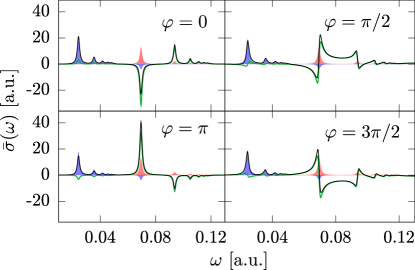
Figure 1: Absorption coefficient $\bar{\sigma}(\omega)$ of the state defined in Eq. (59) with $\varphi=0$, $(1/2)\pi$, $\pi$ and $(3/2)\pi$. The total spectrum (black line) is the sum of two phase-independent terms $0.4\bar{\sigma}_{2p_{z}}$ (red shaded) and $0.6\bar{\sigma}_{3p_{z}}$ (blue shaded) coming from the excited state spectra of the respective states, plus the phase-dependent interference term $\bar{\sigma}^{\mathrm{INT}}(\omega,\varphi)$ (green dashed line), which is responsible for the change of the spectrum with the delay time.

Fig. 1 shows the different contributions and the complete spectrum for $\varphi=0$, $(1/2)\pi$, $\pi$ and $(3/2)\pi$, which are the cases, where the interference term is either purely Lorentzian ($\varphi=0$, $\pi$) or purely Rayleigh ($\varphi=1/2\pi$, $3/2\pi$). The shaded areas indicate the weighted equilibrium contributions, the dotted line shows the interference terms, and the solid line the complete spectrum. The energy range shown includes the transitions from n = 2 to all higher states and from n = 3 to all higher states and to n = 2. Transitions to the ground state lie outside of this region.

As can be learnt from Eq. (79), the interference terms require the existence of states which are dipole-coupled to both $2p_{z}$ and $3p_{z}$. This is the case for $s$- and $d$-orbitals. This means, that e.g. for Hydrogen in a linear combination of the states $2s$ and $4f$, all the interference terms would vanish and the spectrum would be purely the sum of the weighted equilibrium contributions.

Let us take a closer look at the structure of the interference terms. We start with the interference term at $\omega_{23}=0.069$ Ha having contributions from terms with $m=2s$, $m=3s$ and $m=3d$. All contributions have different prefactors with the ones coming from the 2s-state having the opposite sign compared to the ones coming from 3s and 3d states. For the other peaks, the interference terms are much smaller at the energies $\omega_{3n}$ than their counterparts at $\omega_{2n}$ (compare the purely blue to the purely red peaks in Fig. 1). From Eq. (79), it is apparent that the amplitude of each interference term is the same for $\omega_{2n}$ and $\omega_{3n}$ with the same $n$. The difference comes purely from the factor $\frac{4\pi\omega}{3c}$ – note that the sign of the Rayleigh contributions is opposite in these pairs of peaks. This variation of amplitude has the following consequences for the change of the overall spectrum: At $\omega_{3n}$ the spectrum has positive contributions from $\bar{\sigma}_{3p_{z}}$ and contributions from the interference terms, but since the interference terms are much smaller than $\bar{\sigma}_{3p_{z}}$, the spectrum changes only slightly for different $\varphi$’s. This is different for the peaks at energies $\omega_{2n}$. Here, the spectrum has positive, phase-independent contributions from $\bar{\sigma}_{2p_{z}}(\omega)$, but the contributions from the interference terms are much larger and dominate the spectrum leading to a strong dependence of the spectrum in this energy range on the phase $\varphi$. For $\varphi=0$ and $\varphi=\pi$, $\bar{\sigma}^{\rm INT}(\omega,\varphi)$ only contains Lorentzian peaks and consequently the whole spectrum only contains Lorentzians. Nevertheless, $\bar{\sigma}^{\rm INT}(\omega,\varphi)$ changes sign between $\varphi=0$ and $\varphi=\pi$, switching the sign of all peaks at $\omega_{2n}$. This is a demonstration of, how the manipulation of the internal phase $\varphi$ can lead to a switch from gain (negative peaks) to loss (positive peaks) regime and vice versa. Finally, for $\varphi=(1/2)\pi$ and $\varphi=(3/2)\pi$, the interference spectrum contains purely Rayleigh peaks. Together with the small contributions from the stationary-state contributions, the final spectrum consists of slightly asymmetric Rayleigh peaks, again with different signs for $\varphi=(1/2)\pi$ and $\varphi=(3/2)\pi$. One can therefore not only change peaks from emission to absorption peaks, but also manipulate their shape. The phases $\varphi$ therefore play a critical role in the spectral weights and the peaks of the photo-absorption spectrum.

We now look at the variation of the spectrum with time, assuming that an initial, yet unknown pump laser created the state of Eq. (59) with $\varphi=\varphi_{32}=0$ at $t=T$ and we probe the system at different delay times $\tau$. Figure 2 shows the corresponding time-resolved spectrum $\bar{\sigma}(\omega,\tau)$ of $|\bar{\Psi}\rangle$. Since the eigenenergies of $|2p_{z}\rangle$ and $|3p_{z}\rangle$ are different, the phase $\Theta_{32}(\tau)$ in Eq. (27) evolves with the frequency $\omega_{32}$. At $\tau=0$, $\tau=\frac{\pi}{2\omega_{32}}$, $\tau=\frac{\pi}{\omega_{32}}$ and $\tau=\frac{3\pi}{2\omega_{32}}$, the spectra of Fig. 1 are reproduced. One sees the strong changes of $\bar{\sigma}$ in the energy range of the peaks $\omega_{2n}$, while the peaks $\omega_{3n}$ remain almost unchanged. The spectrum is periodic with $T=\frac{2\pi}{\omega_{32}}\approx$ 91 a.u..

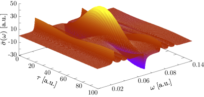
Figure 2: Time-resolved spectrum of the initial state $\sqrt{0.4}|2p_{z}\rangle+\sqrt{0.6}|3p_{z}\rangle$ of Hydrogen. Because the phases of the $|2p\rangle$ and $|3p\rangle$ states evolve with different velocities, the spectral weights of each of the peaks changes with time, leading to a time-dependent spectrum with a periodicity of $T=\frac{2\pi}{\omega_{32}}\approx 91a.u.$.

We now move on to the control problem – i.e. the design of a pump pulse driving the system into a state with specific optical properties. For this problem, we will use the three-levels model, and the analytical equations of control presented in Section III. The target state will again be the one defined in Eq. (59) $|\bar{\Psi}\rangle=\sqrt{0.4}|2p_{z}\rangle+\sqrt{0.6}e^{i\varphi}|3p_{z}\rangle$ with a relative phase of $\varphi=0$: $|\bar{\Psi}\rangle=\sqrt{0.4}|2p_{z}\rangle+\sqrt{0.6}|3p_{z}\rangle$. The three active states are then $|1s\rangle$, $|2p_{z}\rangle$ and $|3p_{z}\rangle$. Note that since $|2p_{z}\rangle$ and $|3p_{z}\rangle$ have the same symmetry, they are decoupled in the dipole approximation, and in consequence the system fits into the framework described in Section III. We may therefore write down the shape of a control pulse, assuming a total pulse time of $T=3200$ a.u:

$$\mathscr{E}(t)=\frac{2\pi}{T} \left(\frac{\sqrt{0.4}}{d_{1s\rightarrow 2p}}\cos(\omega_{1s\rightarrow 2p}(t-T)+\pi)\right.$$ (80)

$$+ \left.\frac{\sqrt{0.6}}{d_{1s\rightarrow 3p}}\cos(\omega_{1s\rightarrow 3p}(t-T)+\pi)\right)\sin^{2}\left(\pi\frac{t}{T}\right).$$

We numerically solved the TSDE in order to check the validity of the three-level approximation. To this end we discretized the equations on a spherical grid of radius $R=60$ a.u., spacing of $\Delta x=0.435$ a.u. and with 20 a.u. wide absorbing boundaries placed at the edges.

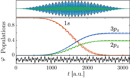
Figure 3: Time-evolution of the populations of the $1s-$, $2p_{z}-$ and $3p_{z}-$ state. Dashed lines show the analytic model, solid lines the numerical results. The total pump-laser (upper panel, black) has two carrier-frequencies, one resonant to the transition $|\Psi_{1s}\rangle\rightarrow|\Psi_{2p}\rangle$ (green), the other resonant to the transition $|\Psi_{1s}\rangle\rightarrow|\Psi_{3p}\rangle$ (blue). The lower panel shows the phase difference $\varphi_{3p}-\varphi_{2p}$.

The results are collected in Figure 3 where we show the time-evolution of the populations $|a(t)|^{2}$, $|b(t)|^{2}$ and $|c(t)|^{2}$ of the states $|1s\rangle$, $|2p_{z}\rangle$ and $|3p_{z}\rangle$ respectively. The numerical values (solid lines) follow closely the ones corresponding to the model (96) (dashed lines) except for a small superimposed oscillatory behavior. A frequency analysis of the additional oscillations shows, that they are due to the components neglected in the rotating wave approximation. The small deviation in the final populations from the analytic prediction comes from the excitation into the 3d-states (not shown). The coupling to these orbitals was neglected in the three-level approximation. This population transfer to the 3d-states nonetheless is less than 4% , and we achieve a transfer into the target wave function $|\bar{\Psi}\rangle$ of 96%. Furthermore the transfer is obtained precisely with the desired relative phase $\varphi=0$ as reported in the bottom panel of Figure 3.

IV.2 More Than one Electron: Results Based on TDDFT

We here turn to systems with more than one electron, and investigate the possibility to drive the absorption of atoms and molecules into the visible using a laser pulse optimized with the gradient-free optimization algorithm presented in Section III in combination with TDDFT.

IV.2.1 Helium

As a first example we study the one-dimensional soft-Coulomb Helium atom. This model is defined by the Hamiltonian:

$$H(t)=T+V_{\rm ext}(t)+V_{\rm ee}\,,$$ (81)

where

$$V_{\rm ext}(t)=-\frac{2}{\sqrt{1+x_{1}^{2}}}-\frac{2}{\sqrt{1+x_{2}^{2}}}+\mathcal{E}(t)(x_{1}+x_{2})$$ (82)

is the external potential with softened Coulomb interaction and the dipolar coupling to the external time-dependent field $\mathcal{E}(t)$ The electron-electron interaction is also described by a soft-Coulomb function $V_{\rm ee}=\frac{1}{\sqrt{1+(x_{1}-x_{2})^{2}}}$. For the optimization we solve the equations discretized on a regular grid of size $L=100$ a.u. and spacing $\Delta x=0.2$ a.u. with 20 a.u. absorbing boundaries at the borders of the simulation box. Results obtained with the optimized pulse were further converged in a box of size $L=200$ a.u. with 70 a.u. absorbing boundaries. Time was discretized with a time step of $\Delta t=0.025$ a.u. for a maximum propagation time of 1250 a.u. during optimization and 2250 a.u. for convergence. The duration of the pump pulse was chosen to be $T_{\mathcal{P}}\leavevmode\nobreak\ =\leavevmode\nobreak\ 800$ a.u. and the delay between pump and probe was set to $\tau=50$ a.u. for all the calculations. Finally the target region for optimization was chosen between 0.06 a.u. and 0.23 a.u. ($\approx$ 200 nm and 800 nm). We carried out optimizations at two different theory levels: exact (TDSE) and TDDFT with the adiabatic EXX functional (TDEXX) Kümmel and Perdew (2003).

Let us first focus on the optimization obtained by solving the exact TDSE as illustrated in Figure 4(b) where the ground state spectra are compared to the spectra of the systems excited by the optimized pump-pulses $\mathscr{E}_{100}(t)$ obtained after 100 iterations. In the exact case, the search space was constructed from two wave lengths $\lambda=800$ nm and $\lambda=1450$ nm and their first nine odd harmonics as shown in Figure 4(a). Optimization is achieved transferring population from the ground state (at $\epsilon_{0}=-2.238$ a.u.) into the first excited state (at $\epsilon_{1}=-1.705$) with the help of the 9th harmonic of $\lambda=1450$ nm at $\omega_{\mathcal{P}13}=0.534$ a.u.. Due to this population transfer, the peak at $\omega_{0\rightarrow 1}=0.533$ a.u. turns from positive to negative and peaks coming from the first excited state ($\omega_{1\rightarrow 2}=0.076$ a.u. and $\omega_{1\rightarrow 4}=0.159$ a.u.) arise in the excited-state spectrum, where the peak at $\omega_{1\rightarrow 2}$ is located in the visible part of the energy range. At the same time, population is transfered into the second excited state ($\epsilon_{2}=-1.629$ a.u.), leading to e.g. the peaks at $\omega_{2\rightarrow 3}=0.062$ a.u. and $\omega_{2\rightarrow 5}=0.103$ a.u.. This interpretation is confirmed by the population analysis in Figure 4(d) where $|\langle\Psi(t)|\Phi_{i}\rangle|^{2}$ is plotted over time. In particular it is apparent that at the end of the pump only $\approx$ 8% of the electrons remain in the ground state, whereas the rest has been transfered into higher lying states thus explaining the appearance of the new peaks in the spectrum. To complete the picture in Figure 4(c) we show the evolution of the control function $G^{A}$ with the number of iterations. As can be seen, $G^{A}$ shows a steady increase during the optimization.

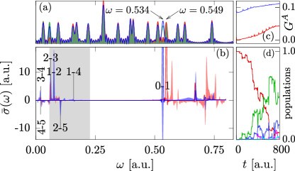
Figure 4: Optimization of the absorption of one-dimensional Helium: TDSE vs. TDEXX. (a) Power spectrum of the initial and optimized laser pulses: The green line shows the initial laser used for the TDSE; the green shaded area shows the initial laser used for the TDEXX optimization (these two only differ by the indicated peaks at $\omega=0.534$ a.u. and $\omega=0.549$ a.u.); the blue and red lines are the optimal pulses obtained when using TDSE and TDEXX, respectively. (b) Ground state (dashed line) and excited state (shaded) spectra of optimized one-dimensional Helium, in blue and red for the TDSE and TDEXX cases, respectively. The excited state transitions of the exact calculations are indicated. (c) The control function $G^{A}$ as a function of the number of iterations, also in blue and red for the TDSE and TDEXX, respectively. (d) The populations $|\langle\Psi(t)|\Psi_{i}\rangle|^{2}$ of the exact time propagation under the influence of the optimized pump pulse for the (red) ground state, (green) first excited state, (blue) second excited state, (pink) third excited state and (turquoise) fourth excited state.

For the TDEXX case we adapted the search space by replacing the laser component at the carrier frequency $\omega=0.534$ a.u. (in resonance with the first excitation in the TDSE case) by a laser component with $\omega=0.549$ a.u., which is its TDEXX equivalent. In our experience failing to meet this requirement resulted in poor optimizations. The resulting optimization is shown in Figure 4(b). The results follow a trend similar to the exact case. However the TDEXX optimization is smaller and the $1\rightarrow 2$ peak present in TDSE seems to be missing. The difference between TDEXX and TDSE can be tracked down to a known problem of the adiabatic approximation in TDDFT. In particular, the lack of memory in the adiabatic approximation, causing a spurious time dependence of the exchange potential, is responsible for the poor population transfer and the excess of asymmetric peaks in the spectrum De Giovannini et al. (2013); Fuks et al. (2015). This problem is further amplified by the ionization of the system, which results in an unphysical shift of the peaks to higher energies (compare the ground state and the excited state spectrum in Figure 4). These effects, however, strongly depend on the fraction of the total density that gets driven out of equilibrium and therefore become more dominant with decreasing size of the system – with Helium being the worst case. In large molecules with many electrons we expect the error to be greatly reduced (as has been empirically shown in studies of light induced charge transfer in organic photovoltaic blends Andrea Rozzi et al. (2013); Falke et al. (2014)).

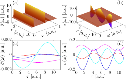
Figure 5: (Top) Transient Absorption Spectrum of Helium after the excitation with a 45 cycle $\sin^{2}$ laser pulse of intensity $I=5.26\cdot 10^{11}Wcm^{-2}$ with a carrier frequency resonant to the excitation energy from the ground to the first excited state for exact (a) and adiabatic EXX (b) with $\omega^{\rm exact}=0.534$ a.u. and $\omega^{\rm EXX}=0.549$ a.u.. Time-evolution of the absorption cross-section at selected energies $\omega_{n}=0.2$ (red), 0.4 (blue), 0.6 (purple) 0.8 (turquoise) a.u. for exact (c) and adiabatic EXX (d). In the exact case the curve at 0.6 a.u. is offset by -0.1 for clarity. In all cases, the time interval $T=2\pi/(\epsilon_{1}-\epsilon_{0})$ is shown.

A different perspective on the same problem can be obtained by comparing the time evolution of an excited state spectrum in TDSE and TDEXX as shown in Figure 5. The systems were excited by a 45 cycle $\sin^{2}$ laser pulse resonant with the excitation energy from the ground state into the first excited state. After the pulse the systems are in a superposition of these two states and the spectra should contain time-dependent interference terms, which oscillate with the period time $T=\frac{2\pi}{\epsilon_{1}-\epsilon_{0}}$, which is $T=11.76$ a.u. for TDSE and $T=11.26$ a.u. for TDEXX. However, on the scale of Figure 5(a) the TDSE spectrum hardly presents any oscillation. Therefore, in Figure 5(c) we report cuts at $\omega_{n}$ = 0.2, 0.4, 0.6 and 0.8 a.u. From the figure it is apparent that, albeit with different phases, each cut presents oscillations with the expected period of $T=11.76$ a.u.. The TDEXX calculations, in Figure 5(b) and (d), present a different picture. First of all, the amplitude of the oscillations is much larger than in the exact case and, second, the oscillations are two times faster than expected. We conclude, that the TDEXX description seems to have a similar structure to the exact case, in the sense, that the energy difference of the involved states is reflected in the periodicity of the oscillations of the spectrum. Nonetheless, there are major differences in the behaviour, which is reflected in the factor of two in the periodicity.

IV.2.2 Methane Dication

Finally, we apply our scheme to a poly-atomic molecule: doubly-ionized Methane, $\mathrm{CH}_{4}^{+2}$. The goal here is to design a laser capable to turn this molecule, transparent in nature, visible. To this end we used the same strategy as we did before for Helium, namely we optimize the laser on a small simulation box and then converge the results with the optimized laser on a larger box. During the optimization routine the simulation box has a radius of $R=15$ a.u., including 5 a.u. absorbing boundaries while the results are converged in a box of $R=30$ a.u. with 15 a.u. absorbing boundaries. We discretize the TDDFT equations on a three-dimensional grid with a spacing of $\Delta x=0.3$ a.u.. The reason for this box choice is the fact that the computational costs of three-dimensional calculations scale with the third power of the simulation box radius. The maximum propagation time is 850 a.u. during the optimization and 1600 a.u. for convergence. In all cases, the pump duration was 600 a.u., the time step was $\Delta t=0.04$ a.u. and the delay was $\tau=0$ a.u..

The optimization region was chosen as the interval between 0.057 a.u. and 0.139 a.u. (328 and 750 nm) and in order to discourage the algorithm from exciting too many electrons into the continuum, we used the target functional $G^{B}_{\tau}$ (51b), which includes an exponential “penalty” for ionization.

To obtain a good description of states close to the ionization threshold, we employed the average density self-interaction corrected (ADSIC) LDA functional Legrand et al. (2002), which is asymptotically correct.

The inclusion of resonant frequencies in the search space is a good practice that facilitates transitions between eigenstates and enables the optimization algorithm to populate excited eigenstates. These molecular excitation frequencies can easily be obtained from the ground-state spectrum reported in Figure 6. By populating the correct eigenstates, the system might absorb in the visible region: consider two eigenstates with energies $\epsilon_{h}$ and $\epsilon_{T}$, that differ by an energy in the visible: 0.057 a.u. $\leq\epsilon_{h}-\epsilon_{T}\leq$ 0.139 a.u.. By exciting the system into the lower “target” state $\epsilon_{T}$ one might obtain transition peaks in the visible, due to the transition to the higher one. Note, however, that this fact is not guaranteed since the transition might be dipole forbidden. We cannot rule out this possibility since our groundstate linear-response TDDFT calculation does not provide this information.

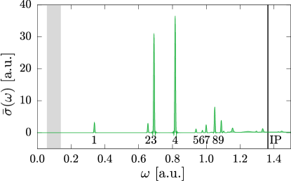
Figure 6: Ground state spectrum of doubly-ionized Methane CH${}_{4}^{2+}$. Peaks are numbered for later reference (as discussed in the text). The shaded grey area marks the optimization range.

The ground state spectrum shows, that the first possible target state is $\epsilon_{3}$. The energy difference between $\epsilon_{3}=0.690$ a.u. and $\epsilon_{4}=0.816$ a.u. is $\omega_{3\rightarrow 4}=0.126$ a.u. and lies – with 362 nm – at the red end of the visible spectrum. Also $\epsilon_{4}$ provides a transition in the visible range – into $\epsilon_{5}=0.938$ a.u. with $\omega_{4\rightarrow 5}=0.122$ a.u. = 373 nm. Starting from $\epsilon_{5}$, the states have even more than one transition in the visible. We must therefore choose a frequency search space, that allows the construction of a pump pulse, that excites electrons from the ground state into $\epsilon_{3}$ and higher lying states either directly or by successive excitations.

Here we present results for two possible search spaces. The first search space includes frequencies that are either resonant to the ground state excitation energies $\epsilon_{n}$, or to excited state excitations $\epsilon_{m}-\epsilon_{n}$. To avoid ionization, all carrier frequencies are smaller than $\epsilon_{7}=1.0$ a.u.. The second frequency search space was designed using the ionization potential $I_{P}$ of the system (which is equal to minus the energy $\epsilon_{H}$ of the highest occupied KS orbital $\varphi_{H}$) and the energy differences $I_{P}-\epsilon_{n}$. One frequency is $I_{P}$ itself, while all others are resonant with relaxations bringing down states at that ionization threshold to bound excited states ($\epsilon_{3}$ to $\epsilon_{8}$). The idea is that the system could be excited into the ionization threshold, and then relax into one of the target states. The laser frequencies, that were included in the search spaces and the corresponding resonances are summarized in Appendix C.

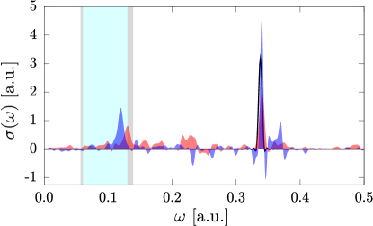
Figure 7: Ground state (black line) and excited state (shaded) spectra of doubly-ionized Methane (CH${}_{4}^{2+}$) for two different pump pulses $\mathscr{E}^{I}$ (red) and $\mathscr{E}^{II}$ (blue). The grey shaded box marks the optimization area, the blue shaded area the visible region of the spectrum.

The optimized spectra are shown in Figure 7. It can be seen that both search spaces include optimal lasers that cause the molecule to loose its transparency and absorb in the visible. The achieved opacity can be quantified in terms of the control function $G^{A}$ (51b) being the integral over the absorption spectrum in the visible range of the spectrum. Comparing the opacity achieved in search space I ($G^{A}_{I}=0.017$) with the one achieved in search space II ($G^{A}_{II}=0.020$), we conclude that search space II is better suited for the pursued optimization. Thus, including energy levels at the ionization threshold in the search space might be a useful strategy in further optimizations.

V Conclusions

In this work, we assessed the possibility of using tailored pumps in order to enhance some given features of the probe absorption – for example, the absorption in the visible range of otherwise transparent samples. We first detailed a theoretical analysis of the non-equilibrium response function in this context, aided by one simple numerical model of the Hydrogen atom. Then, we investigated the feasibility of using TDDFT theory as a means to implement, theoretically, this absorption-optimization idea, for more complex atoms or molecules.

The theoretical analysis of the response function can be done by writing it in a generalized form of the Lehmann representation, valid for systems that have been pumped out of equilibrium by a first pulse, and whose response to a probe pulse (in our case, assumed non-overlapping with the first one) needs to be studied and manipulated. The peaks of this response functions are always fixed to the differences in the system energies, but their strength and shape varies depending on the pump shape, and on the pump-probe delay. Furthermore, the response function is a sum of a stationary part (the only one present if the pumped state is itself a stationary state), and a time-dependent, oscillatory term, caused by interferences between the populated eigenstates.

We then used this dependence of the non-equilibrium response with respect to the pump pulse shape to manipulate it by means of QOCT. We demonstrated the idea first with a small model, that could be treated analytically. This could be a viable alternative for larger systems, if they can be reduced to few-level models. However, for full generality we also showed how QOCT can be combined with TDDFT. We showed how this avenue is tractable, but we also highlighted the key numerical difficulties and theoretical challenges. For this purpose, we performed first calculations on a model for the Helium atom that could be solved both exactly with the TDSE equation, and with TDDFT within the adiabatic EXX approximation. Then we concluded with simulations of the methane dication.

From our results we conclude that the proposed idea could be brought to the laboratory: tailored pump pulses can excite systems into light-absorbing states. Theoretically, the scalability of TDDFT could in principle permit studying these processes for larger systems. However, our results have also highlighted the severe numerical and theoretical difficulties posed by the problem: large-scale non-equilibrium quantum dynamics are cumbersome, even with TDDFT, and moreover the shortcomings of state-of-the-art TDDFT functionals may still be serious for these out-of-equilibrium situations. Our findings confirm recent investigations about the consequences of these shortcomings for the use of coherent control schemes Raghunathan and Nest (2011, 2012).

Appendix A Quantum Optimal Control Equations

For completeness, we derive here the equations for the computation of the gradient of a target functional designed to optimize the response of a system. In general, the equation for the gradient provided by QOCT is given by:

$$\nabla_{\mathbf{c}} G[\mathbf{c}]=\left.\nabla_{\mathbf{c}}F[\Psi,\mathscr{E}_{\mathbf{c}}]\right|_{\Psi=\Psi[\mathscr{E}_{\mathbf{c}}]}+$$

$$2\Im\int_{0}^{T}\!\!\!{\rm d}t\;\langle\chi[\mathscr{E}_{\mathbf{c}}](t)|\nabla_{\mathbf{c}}\hat{H}[\mathscr{E}_{\mathbf{c}},t]|\Psi[\mathscr{E}_{\mathbf{c}}](t)\rangle\,$$ (83a)

Note that a new “wave function”, $\chi[\mathscr{E}]$, has been introduced; it is given by the solution of:

$$i\frac{\partial\chi[\mathscr{E}]}{\partial t}(x,t) = \hat{H}^{\dagger}[\mathscr{E},t]\chi[\mathscr{E}](x,t)$$ (83b)

$$\chi[\mathscr{E}](x,T) = \frac{\delta J_{1}^{T}}{\delta\Psi^{*}[\mathscr{E}](x,T)}\,.$$ (83c)

This is similar to the original Schrödinger equation (47), although the initial condition is given at the final time $t=T$, which implies it must be propagated backwards. For a detailed derivation of Eqs. (83) we refer the reader to Refs. Peirce et al. (1988); Kosloff et al. (1989); Ohtsuki et al. (2004); Serban et al. (2005).

The computation of the gradient or functional derivative of $G$, therefore, requires $\Psi[\mathscr{E}]$ and $\chi[\mathscr{E}]$, which are obtained by first propagating Eq. (47a) forwards, and then Eq. (83b) backwards. The maxima of $G$ are found at the critical points $\nabla_{\mathbf{c}}G[\mathscr{E}_{\mathbf{c}}]=0$.

We may now apply these general equations for a target functional designed to optimize the response of a system after the excitation by a pump pulse. This setup is consistent with the non-overlapping regime described in Section II, where the Hamiltonian that governs the system, once that the pump has passed ($t\geq T$) has the form (1). If, at time $t=T$, the system has been driven to the state $|\Psi(T)\rangle$, the response function for the perturbation at later times is given by (II) and the first-order response of the system is given by (4).

The key point is the definition of a target: for example, let us assume, that we wish to enhance the reaction of the system at a given frequency to a sudden perturbation at the end of the pump $F(t^{\prime})=\delta(t-T)$. As seen in (5), the time-dependent dipole-dipole response is then directly given by the response function $\chi_{\hat{D},\hat{D}}\left[\mathscr{E}\right](t,T)=D^{(1)}\left[\mathscr{E},\delta_{T}\right](t)$ and its Fourier transform by

$$\chi_{\hat{D},\hat{D}}\left[\mathscr{E}\right](\omega,T) = D^{(1)}\left[\mathscr{E},\delta_{T}\right](\omega)$$ (84)

$$= \int_{T}^{\infty}\!\!{\rm dt^{\prime}}\;e^{-i\omega t^{\prime}}D^{(1)}\left[\mathscr{E},\delta_{T}\right](t^{\prime})\,.$$

It can be easily seen that the problem fits into the framework discussed above, i.e. the target functional is given by the expectation value of some operator:

$$J_{1}^{T}[\Psi(T)]=-i$$

$$\langle\Psi(T)|\int_{T}^{\infty}\!\!{\rm dt^{\prime}}\;e^{-i\omega t^{\prime}}\left[e^{i(t^{\prime}-T)\mathscr{H}}\hat{D}e^{-i(t^{\prime}-T)\mathscr{H}},\hat{D}\right]|\Psi(T)\rangle\,.$$ (85)

The equation for the gradient is therefore Eq. (83a); which must be completed with the equation of motion for the co-state, Eq. (83b), and, in particular, with its boundary condition (83c) at time $t=T$: this is the only one that in fact depends on the definition of the target operator:

$$|\chi(T)\rangle=-i$$

$$\int_{T}^{\infty}\!\!{\rm dt^{\prime}}\;e^{-i\omega t^{\prime}}\left[e^{i(t^{\prime}-T)\mathscr{H}}\hat{D}e^{-i(t^{\prime}-T)\mathscr{H}},\hat{D}\right]|\Psi(T)\rangle\,.$$ (86)

Similar formulas can be obtained for more general definitions of the target functional in terms of the response $D^{(1)}(\omega)$, and for more general probe functions. In all cases the computational difficulties associated to the computation of this boundary condition are similar, and are considerable. By inspecting the previous formula, it can be learnt that various time-propagations of the wave functions, forwards and backwards, are required. These difficulties are even larger if the scheme is formulated within TDDFT – in the previous derivation we have used the exact many-electron wave functions. In consequence, we decided to employ, for this type of optimizations, gradient-free algorithms, such as the Simplex-Downhill algorithm that we describe in next section.

Appendix B Derivation of the Control Equations for Three Level Systems

For the three-levels model described at the end of Section III, we will start by considering a simpler situation in which the field envelopes are constant, i.e.:

$$\mathscr{E}(t)=\varepsilon_{1}\cos(\omega_{1}t+\varphi_{1})+\varepsilon_{2}\cos(\omega_{2}t+\varphi_{2})\,.$$ (87)

If the two carrier frequencies are sufficiently close to the transition frequencies $\omega_{ab}$ and $\omega_{bc}$, one can apply the rotating wave approximation (RWA), as it is done in the theory of Rabi oscillations. In fact, we choose the carrier frequencies to be equal to the transition energies. In addition, we also assume, that the laser frequencies are sufficiently well separated in energy to apply the RWA a second time:

$$|\omega_{1}+\omega_{2}| \gg 0\,,$$ (88a)

$$|\omega_{1}-\omega_{2}| \gg 0\,.$$ (88b)

Assuming the validity of the RWA mentioned in Section III, the solution of the resulting differential equations with the initial conditions $a(0)=1$, $b(0)=c(0)=0$, leads to the following time-evolution of the coefficients:

$$a(t) = \cos(\bar{\Omega}/2t)\,,$$ (89a)

$$b(t) = \frac{d_{ab}\varepsilon_{1}e^{-i(\varphi_{1}-\pi)}}{\sqrt{(d_{ab}\varepsilon_{1})^{2}+(d_{ac}\varepsilon_{2})^{2}}}\sin\left(\bar{\Omega}/2t\right)\,,$$ (89b)

$$c(t) = \frac{d_{ac}\varepsilon_{2}e^{-i(\varphi_{2}-\pi)}}{\sqrt{(d_{ab}\varepsilon_{1})^{2}+(d_{ac}\varepsilon_{2})^{2}}}\sin\left(\bar{\Omega}/2t\right)\,,$$ (89c)

with the Rabi-frequency

$$\bar{\Omega}=\sqrt{(d_{ab}\varepsilon_{1})^{2}+(d_{ac}\varepsilon_{2})^{2}}\,.$$ (90)

Note that:

1. The Rabi-frequency is the Pythagorean mean of the Rabi-frequencies of the single transitions: $\bar{\Omega}=\sqrt{\bar{\Omega}_{ab}^{2}+\bar{\Omega}_{ac}^{2}}$. Consequently, it is larger than each of those single frequencies.

2. The maximum populations of the excited states depend only on the ratio of the Rabi-frequencies belonging to the respective transitions $\frac{|b(t)|^{2}}{|c(t)|^{2}}=\frac{\bar{\Omega}_{ab}^{2}}{\bar{\Omega}_{ac}^{2}}$.

3. The relative phases of the expansion coefficients depend on the phases of the applied lasers.

The target state is defined in Eq. (54): the goal is to find a laser pulse that drives the system from the state $|\Psi(t=0)\rangle=|\Phi_{a}\rangle$ into this target state within the time $T$. The evolution of the time-dependent wave function is given by:

$$|\Psi(t)\rangle =\cos(\bar{\Omega}/2t)|\Phi_{a}\rangle$$

$$+\frac{d_{ab}\varepsilon_{1}\sin\left(\bar{\Omega}/2t\right)}{\sqrt{(d_{ab}\varepsilon_{1})^{2}+(d_{ac}\varepsilon_{2})^{2}}}e^{-i(\varphi_{1}-\pi+\omega_{ba}t)}|\Phi_{b}\rangle$$

$$+\frac{d_{ac}\varepsilon_{2}\sin\left(\bar{\Omega}/2t\right)}{\sqrt{(d_{ab}\varepsilon_{1})^{2}+(d_{ac}\varepsilon_{2})^{2}}}e^{-i(\varphi_{2}-\pi+\omega_{ca}t)}|\Phi_{c}\rangle\,.$$ (91)

The condition $|\langle\Phi_{a}|\bar{\Psi}\rangle|^{2}=1$ leads to two sets of equations: one connecting the laser amplitudes $\varepsilon_{1}$ and $\varepsilon_{2}$ to the populations $|\alpha|^{2}$, $|\beta|^{2}$ and $|\gamma|^{2}$

$$|\alpha| = \cos(\bar{\Omega}/2T)\,,$$ (92a)

$$|\beta| = \frac{d_{ab}\varepsilon_{1}}{\sqrt{(d_{ab}\varepsilon_{1})^{2}+(d_{ac}\varepsilon_{2})^{2}}}\sin\left(\bar{\Omega}/2T\right)\,,$$ (92b)

$$|\gamma| = \frac{d_{ac}\varepsilon_{2}}{\sqrt{(d_{ab}\varepsilon_{1})^{2}+(d_{ac}\varepsilon_{2})^{2}}}\sin\left(\bar{\Omega}/2T\right)\,,$$ (92c)

and the other one connecting the laser phases to the relative phases $\varphi_{\beta}$ and $\varphi_{\gamma}$ of the wave function

$$\varphi_{\beta} = \varphi_{1}-\pi+\omega_{ba}T\,,$$ (93a)

$$\varphi_{\gamma} = \varphi_{2}-\pi+\omega_{ca}T\,.$$ (93b)

Solving these sets of equations, we find the following amplitudes as one example of a control laser

$$\varepsilon_{1} = \frac{2}{T}\frac{\arccos(|\alpha|)}{\sin(\arccos(|\alpha|)}\frac{|\beta|}{d_{ab}}\,,$$ (94)

$$\varepsilon_{2} = \frac{2}{T}\frac{\arccos(|\alpha|)}{\sin(\arccos(|\alpha|)}\frac{|\gamma|}{d_{ac}}\,.$$ (95)

Note, however, that the solutions are not unique: other sets $\{(2n+1)\varepsilon_{1},(2n+1)\varepsilon_{2}\}$ fulfill the equations above. These solutions represent lasers that lead to an evolution of the coefficients that covers $(n+1)$ complete Rabi cycles within the time $T$.

In practice one is often interested in pulses with time-dependent envelope functions, such as the ones discussed in Section III, in which the pulses have a $\sin^{2}$ envelope with a period of $2T$. The problem can be solved in an analogue manner; the solutions for the amplitudes were already given in Section III. In this case, the evolution of the coefficients is given by:

$$a(t) = \cos\left(\frac{\int_{0}^{t}\tilde{\Omega}(t^{\prime})dt^{\prime}}{2}\right)\,,$$ (96a)

$$b(t) = \frac{d_{ab}\varepsilon_{1}e^{-i(\varphi_{1}-\pi)}}{\sqrt{(d_{ab}\varepsilon_{1})^{2}+(d_{ac}\varepsilon_{2})^{2}}}\sin\int_{0}^{t}\frac{\tilde{\Omega}(t^{\prime})dt^{\prime}}{2}\,,$$ (96b)

$$c(t) = \frac{d_{ac}\varepsilon_{2}e^{-i(\varphi_{2}-\pi)}}{\sqrt{(d_{ab}\varepsilon_{1})^{2}+(d_{ac}\varepsilon_{2})^{2}}}\sin\int_{0}^{t}\frac{\tilde{\Omega}(t^{\prime})dt^{\prime}}{2}\,,$$ (96c)

where the “time-dependent Rabi-frequency” $\tilde{\Omega}(t)$ is given by:

$$\tilde{\Omega}(t)=\sqrt{(d_{ab}\tilde{\varepsilon}_{1}(t))^{2}+(d_{ac}\tilde{\varepsilon}_{2}(t))^{2}}=2\bar{\Omega}\sin^{2}\left(\pi\frac{t}{T}\right)\,.$$ (97)

and integrates as:

$$\int_{0}^{t}\frac{\tilde{\Omega}(t^{\prime})dt^{\prime}}{2}=\left(\frac{1}{2}t-\frac{T}{4\pi}\sin\left(2\pi\frac{t}{T}\right)\right)\bar{\Omega}\,.$$ (98)

Appendix C Laser Frequencies Used in the Optimization of Methane

The laser frequencies (in a.u.) and the corresponding resonances of the search spaces of the optimization of CH${}_{4}^{2+}$. The nomenclature follows the one in Fig. 6: $\epsilon_{H}$ is minus the energy of the highest occupied KS state. $\omega_{3}^{I}$ is the average of $\epsilon_{1}=0.337$ a.u. and $\epsilon_{3}-\epsilon_{1}=0.353$ a.u.. Since the frequencies are broadened by the finite pulse duration, $\omega_{3}^{I}$ covers both resonances.

Search Space I
$\omega_{1}^{I}$	$\omega_{2}^{I}$	$\omega_{3}^{I}$	$\omega_{4}^{I}$	$\omega_{5}^{I}$
0.122	0.248	0.345	0.479	0.601
$\epsilon_{4}-\epsilon_{5}$	$\epsilon_{3}-\epsilon_{5}$	$\epsilon_{1}$ / $\epsilon_{1}-\epsilon_{3}$	$\epsilon_{1}-\epsilon_{4}$	$\epsilon_{1}-\epsilon_{5}$
$\omega_{6}^{I}$	$\omega_{7}^{I}$	$\omega_{8}^{I}$	$\omega_{9}^{I}$	$\omega_{10}^{I}$
0.654	0.690	0.816	0.938	1.000
$\epsilon_{2}$	$\epsilon_{3}$	$\epsilon_{4}$	$\epsilon_{5}$	$\epsilon_{7}$

Search Space II
$\omega^{II}_{1}$	$\omega^{II}_{2}$	$\omega^{II}_{3}$	$\omega^{II}_{4}$	$\omega^{II}_{5}$	$\omega^{II}_{6}$	$\omega^{II}_{7}$
0.311	0.364	0.386	0.426	0.548	0.674	1.364
$\epsilon_{3}-I_{P}$	$\epsilon_{4}-I_{P}$	$\epsilon_{5}-I_{P}$	$\epsilon_{6}-I_{P}$	$\epsilon_{7}-I_{P}$	$\epsilon_{8}-I_{P}$	$I_{P}$

References

- Krausz and Ivanov (2009) F. Krausz and M. Ivanov, Rev. Mod. Phys. 81, 163 (2009).
- Scrinzi et al. (2006) A. Scrinzi, M. Y. Ivanov, R. Kienberger, and D. M. Villeneuve, Journal of Physics B: Atomic, Molecular and Optical Physics 39, R1 (2006).
- Zewail (1994) A. Zewail, Femochemistry Volume I and II (World Scientific, Singapore, 1994).
- Zewail (2000) A. Zewail, J. Phys. Chem. A 104, 5660 (2000).
- Berera et al. (2009) R. Berera, R. van Grondelle, and J. T. M. Kennis, Photosynth. Res. 101, 101 (2009).
- Foggi et al. (2001) P. Foggi, L. Bussotti, and F. V. R. Neuwahl, International Journal of Photoenergy , 103 (2001).
- Pfeifer et al. (2008) T. Pfeifer, M. J. Abel, P. M. Nagel, A. Jullien, Z.-H. Loh, M. J. Bell, D. M. Neumark, and S. R. Leone, Chemical Physics Letters 463, 11 (2008).
- Goulielmakis et al. (2010) E. Goulielmakis, Z.-H. Loh, A. Wirth, R. Santra, N. Rohringer, V. S. Yakovlev, S. Zherebtsov, T. Pfeifer, A. M. Azzeer, M. F. Kling, S. R. Leone, and F. Krausz, Nature 466, 739 (2010).
- Holler et al. (2011) M. Holler, F. Schapper, L. Gallmann, and U. Keller, Phys. Rev. Lett. 106, 123601 (2011).
- Runge and Gross (1984) E. Runge and E. Gross, Physical Review Letters 52, 997 (1984).
- Marques et al. (2011) M. A. L. Marques, N. T. Maitra, F. Nogueira, E. K. U. Gross, and A. Rubio, Fundamentals of Time-Dependent Density Functional Theory (Springer-Verlag, 2011).
- (12) See the special issue of Chemical Physics 2011, 391, guest-edited by R. Baer, L. Kronik, S. Kümmel.
- De Giovannini et al. (2012) U. De Giovannini, D. Varsano, M. A. L. Marques, H. Appel, E. K. U. Gross, and A. Rubio, Physical Review A 85, 062515 (2012).
- De Giovannini et al. (2013) U. De Giovannini, G. Brunetto, A. Castro, J. Walkenhorst, and A. Rubio, ChemPhysChem 14, 1363 (2013).
- Brif et al. (2010) C. Brif, R. Chakrabarti, and H. Rabitz, New Journal of Physics 12, 075008 (2010).
- Werschnik and Gross (2007) J. Werschnik and E. Gross, Journal of Physics B: Atomic, Molecular and Optical Physics 40, R175 (2007).
- Shi et al. (1988) S. Shi, A. Woody, and H. Rabitz, The Journal of chemical physics 88, 6870 (1988).
- Peirce et al. (1988) A. P. Peirce, M. A. Dahleh, and H. Rabitz, Phys. Rev. A 37, 4950 (1988).
- Kosloff et al. (1989) R. Kosloff, S. Rice, P. Gaspard, S. Tersigni, and D. Tannor, Chemical Physics 139, 201 (1989).
- Luenberger (1969) D. G. Luenberger, Optimization by vector space methods (John Wiley & Sons, Inc., New York, 1969).
- Luenberger (1979) D. G. Luenberger, Introduction to Dynamic Systems (John Wiley & Sons, Inc., New York, 1979).
- Brumer and Shapiro (1986a) P. Brumer and M. Shapiro, Chemical Physics Letters 126, 541 (1986a).
- Brumer and Shapiro (1986b) P. Brumer and M. Shapiro, Faraday Discussions of the Chemical Society 82, 177 (1986b).
- Shapiro and Brumer (2003) M. Shapiro and P. Brumer, Principles of the Quantum Control of Molecular Processes (Wiley, New York, 2003).
- Tannor and Rice (1985) D. J. Tannor and S. A. Rice, The Journal of Chemical Physics 83, 5013 (1985).
- Herek et al. (1994) J. Herek, A. Materny, and A. Zewail, Chemical Physics Letters 228, 15 (1994).
- Gaubatz et al. (1988) U. Gaubatz, P. Rudecki, M. Becker, S. Schiemann, M. Külz, and K. Bergman, Chemical Physics Letters 149, 463 (1988).
- Ohmori (2009) K. Ohmori, Annual Review of Physical Chemistry 60, 487 (2009), pMID: 19335221.
- Judson and Rabitz (1992) R. S. Judson and H. Rabitz, Phys. Rev. Lett. 68, 1500 (1992).
- Bardeen et al. (1997) C. J. Bardeen, V. V. Yakovlev, K. R. Wilson, S. D. Carpenter, P. M. Weber, and W. S. Warren, Chemical Physics Letters 280, 151 (1997).
- Assion et al. (1998) A. Assion, T. Baumert, M. Bergt, T. Brixner, B. Kiefer, V. Seyfried, M. Strehle, and G. Gerber, Science 282, 919 (1998).
- Castro et al. (2012) A. Castro, J. Werschnik, and E. K. U. Gross, Phys. Rev. Lett. 109, 153603 (2012).
- Hellgren et al. (2013) M. Hellgren, E. Räsänen, and E. K. U. Gross, Phys. Rev. A 88, 013414 (2013).
- Castro (2013) A. Castro, ChemPhysChem 14, 1488 (2013).
- Castro and Gross (2014) A. Castro and E. K. U. Gross, Journal of Physics A: Mathematical and Theoretical 47, 025204 (2014).
- Krieger et al. (0) K. Krieger, J. K. Dewhurst, P. Elliott, S. Sharma, and E. K. U. Gross, Journal of Chemical Theory and Computation 0, null (0).
- Harris et al. (1990) S. E. Harris, J. E. Field, and A. Imamoğlu, Phys. Rev. Lett. 64, 1107 (1990).
- Fleischhauer et al. (2005) M. Fleischhauer, A. Imamoglu, and J. P. Marangos, Rev. Mod. Phys. 77, 633 (2005).
- Alexander L. Fetter (2003) J. D. W. Alexander L. Fetter, Quantum Theory of Many-Particle Systems (Dover Publications, 2003).
- Perfetto and Stefanucci (2015) E. Perfetto and G. Stefanucci, Phys. Rev. A 91, 033416 (2015).
- Zielinski et al. (2014) A. Zielinski, V. P. Majety, S. Nagele, R. Pazourek, J. Burgdörfer, and A. Scrinzi, (2014), 1405.4279 .
- Nelder and Mead (1965) J. A. Nelder and R. Mead, The Computer Journal 7, 308 (1965).
- Kohn (1999) W. Kohn, Rev. Mod. Phys. 71, 1253 (1999).
- Kohn and Sham (1965) W. Kohn and L. J. Sham, Phys. Rev. 140, A1133 (1965).
- Marques et al. (2012) M. A. Marques, M. J. Oliveira, and T. Burnus, Computer Physics Communications 183, 2272 (2012).
- Marques et al. (2003) M. A. Marques, A. Castro, G. F. Bertsch, and A. Rubio, Computer Physics Communications 151, 60 (2003).
- Kümmel and Perdew (2003) S. Kümmel and J. Perdew, Physical Review B 68 (2003).
- Fuks et al. (2015) J. I. Fuks, K. Luo, E. D. Sandoval, and N. T. Maitra, Physical Review Letters 114, 183002 (2015).
- Andrea Rozzi et al. (2013) C. Andrea Rozzi, S. Maria Falke, N. Spallanzani, A. Rubio, E. Molinari, D. Brida, M. Maiuri, G. Cerullo, H. Schramm, J. Christoffers, and C. Lienau, Nat Commun 4, 1602 (2013).
- Falke et al. (2014) S. M. Falke, C. A. Rozzi, D. Brida, M. Maiuri, M. Amato, E. Sommer, A. De Sio, A. Rubio, G. Cerullo, E. Molinari, and C. Lienau, Science 344, 1001 (2014), http://www.sciencemag.org/content/344/6187/1001.full.pdf .
- Legrand et al. (2002) C. Legrand, E. Suraud, and P.-G. Reinhard, Journal of Physics B: Atomic, Molecular and Optical Physics 35, 1115 (2002).
- Raghunathan and Nest (2011) S. Raghunathan and M. Nest, Journal of Chemical Theory and Computation 7, 2492 (2011), pMID: 26606623, http://dx.doi.org/10.1021/ct200270t .
- Raghunathan and Nest (2012) S. Raghunathan and M. Nest, Journal of Chemical Theory and Computation 8, 806 (2012), pMID: 26593342, http://dx.doi.org/10.1021/ct200905z .
- Ohtsuki et al. (2004) Y. Ohtsuki, G. Turinici, and H. Rabitz, The Journal of Chemical Physics 120, 5509 (2004).
- Serban et al. (2005) I. Serban, J. Werschnik, and E. K. U. Gross, Phys. Rev. A 71, 053810 (2005).