A nonlinear impact: evidences of causal effects of social media on market prices

Abstract

Online social networks offer a new way to investigate financial markets’ dynamics by enabling the large-scale analysis of investors’ collective behavior. We provide empirical evidence that suggests social media and stock markets have a nonlinear causal relationship. We take advantage of an extensive data set composed of social media messages related to DJIA index components. By using information-theoretic measures to cope for possible nonlinear causal coupling between social media and stock markets systems, we point out stunning differences in the results with respect to linear coupling. Two main conclusions are drawn: First, social media significant causality on stocks’ returns are purely nonlinear in most cases; Second, social media dominates the directional coupling with stock market, an effect not observable within linear modeling. Results also serve as empirical guidance on model adequacy in the investigation of sociotechnical and financial systems.

1 Introduction

Investors’ decisions are modulated not only by companies’ fundamentals but also by personal beliefs, peers influence and information generated from news and the Internet. Rational and irrational investor’s behavior and their relation with the market efficiency hypothesis [1] have been largely debated in the economics and financial literature [2]. However, it was only recently that the availability of vast amounts of data from online systems paved the way for the large-scale investigation of investor’s collective behavior in financial markets.

Testing for nonlinear dependence is of great importance in financial econometrics due to its implications in model adequacy, market efficiency, and predictability [3]. Taking social media as a proxy for investor’s collective attention over the stock market, we provide empirical evidence that characterize social media impact on market prices as nonlinear.

Previous studies have investigated the predictive power of online expressed opinions and measures of collective attention on market movements . News are perhaps the most explored source of information, especially after the availability of electronically transmitted services and machine readable news [4, 5, 6, 7, 8, 9, 10, 11, 12, 13, 14, 15]. The use of search engines [16, 17, 18, 19, 20, 9, 21] and Wikipedia [22] are examples of the extension of this investigation to broader types of online systems. In addition to that, social media and micro-blogging platforms play an increasingly significant role as proxies of collective intelligence and sentiment of the real world. Not only do they mimic real-world peer-to-peer relationships but they also provide a fine-grained real-time information channel that include stories, facts and shifts in collective opinion. Nonetheless, to what extent this information flood reflects financial dynamics is a relatively novel topic under great debate [23, 19, 15, 24, 25, 26, 27, 28, 29, 30, 9, 31, 32, 33, 34].

Recent developments have shown the importance of Twitter as an information channel about financial markets. An example is the U.S. Securities and Exchange Commission allowance of official company’s disclosure via Twitter in compliance with Regulation Fair Disclosure [35]. Several research evidences also indicate that Twitter may describe and predict financial dynamics. Among the first and most influential works is Bollen et al. (2011) [23], where the authors used emotion analytics to forecast movements in the DJIA index. Later on, in a report for the European Central Bank, the same authors [19] showed that Twitter collective opinion not only has predictive power over stocks’ returns but it actually precedes changes in search volume (Google Trends), a known predictor of economic indicators. Further, Zheludev et al. (2014) [24] showed that Twitter can contain statistically-significant lead-time information about securities’ returns, most remarkably over future prices of the S&P500 index. Sprenger et al. (2014) [25] proposed a methodology that quantified the impact of Twitter messages in the market as well as identified different types of company specific events. Subsequent research by Ranco et al. (2015) [26] reinforced these results while analyzing links among Twitter peaks, excess of stocks’ returns and the identification of earnings announcements.

These recent works provide evidence that exogenous information gathered from sociotechnical systems may be useful to describe financial dynamics. However, the current body of the literature presents mixed results on the stocks’ returns predictability. On the one hand, some researches indicate predictability of price movements using News and social media [4, 5, 23, 19]. On the other hand, other studies report weak results [26, 24] suggesting that social media analytics have low power when used alone. Moreover, the use of ad hoc functional forms and assumptions in different studies makes it difficult to draw general conclusions about the nature of the relationship between sociotechnical systems and stock markets.

We take advantage of an information-theoretic framework to study the causality between social media and stock returns in a nonparametric way. We detect directional and dynamical coupling while not assuming any particular type of interaction between the systems. To our knowledge, our results provide the first empirical evidence that suggests social media and stock markets not only have significant lead-time coupling but also are dominated by nonlinear interactions.

2 Data Analyzed

Our analysis is conducted on the 30 components of the Dow Jones Industrial Average (DJIA) index, which we monitored during the two-year period from March 31, 2012 to March 31, 2014. The choice of these stocks was due to their representativeness of the stock market (see Supporting Information SI.A.1 for the complete list of companies). We consider two streams of time series data: (i) market data, which are given at the daily stock price, and (ii) social media data analytics based on 1,767,997 Twitter messages. Let $P(t)$ be the closing price of an asset at day $t$, as financial variable we consider the stocks’ daily log-returns: $R(t)=\log{P(t)}-\log{P(t-1)}$.

We consider Twitter data analytics as a proxy for the collective opinion over a stock. As opinion mining [36] per se is out of scope of this study, we build our analysis on top of Twitter data analytics supplied by PsychSignal.com [37]. PsychSignal’s natural language processing (NLP) uses a sophisticated linguistic based approach to sentiment mining that is able to extract and score the nuanced financial language used by traders in online conversations.

We take the daily total number of bullish tweets related to a company as the social media time series $SM(t)$. Fig. 1 shows the volume of bearish and bullish messages for the selected companies. A company is defined to be related to a given message if its ticker-id is mentioned as a cashtag, i.e., with its name preceded by a dollar symbol, e.g., $CSCO for the company CISCO SYSTEMS INC. In Twitter, a cashtag is a standard way to refer to a listed security. See Supporting Information SI.A.2 for further details on the Twitter data analytics.

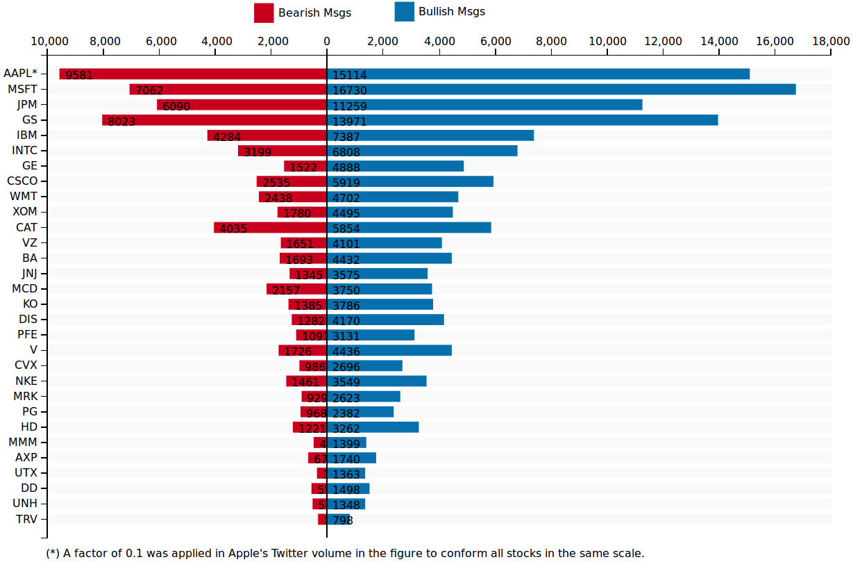
Figure 1: Volume of bearish and bullish Twitter messages mentioning a ticker of a stock component of the DJIA index.

3 Social Media and Stocks’ Returns: Linear and Nonlinear Causality

We investigate the characterization of causal inference between social media and stocks’ returns under the notion of Granger (G-causality) [38, 39]. We test the null hypothesis of social media not causing stocks’ returns. Firstly, we verify this hypothesis with a standard G-causality test under a linear vector-autoregressive framework. This linear model is tested against misspecification via a BDS test [40] which is a nonparametric method that is powerful to detect nonlinearity [41]. Secondly, we detect significant causalities in possible nonlinear dynamical interactions. This is done without assuming any a priori type of interaction. We consider Transfer Entropy (TE) as the measure for nonparametric causality. Since its introduction by Schreiber (2000) [42], TE has been recognized as an important tool in the analysis of causal relationships in nonlinear systems [43]. It naturally detects directional and dynamical information [44]. This measure can be interpreted as the information flow between social media and future outcomes of stocks’ returns at lag $\Delta t$, controlled by current information on stocks’ returns.

Consistent with a nonparametric analysis, we estimate the TE significance via randomized permutation tests. If the null hypothesis is rejected, there is evidence of nonlinear causality, otherwise we consider that there is no significant causality. The hypothesis tests are performed for lags $\Delta t$ ranging from 1 to 10 trading days. We apply the Bonferroni correction to reduce the probability of a Type I (false positive) error due to multiple hypotheses testing.

Social Media $\rightarrow$ Stocks’ Returns

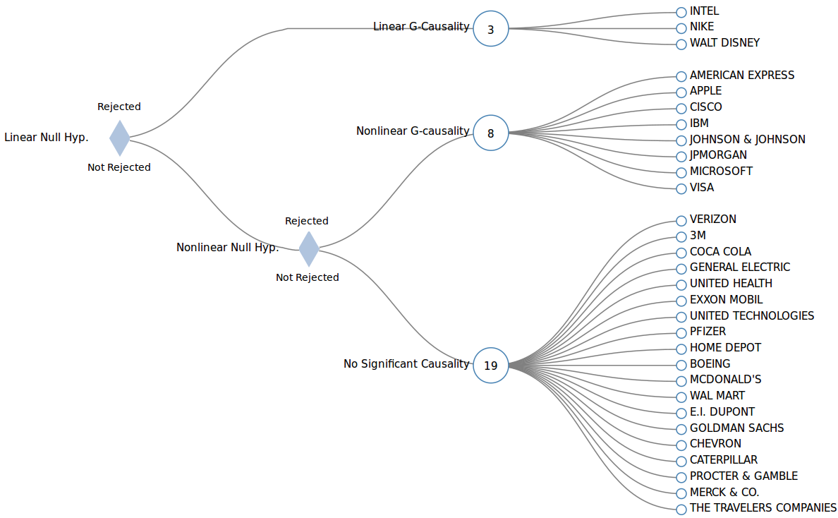
Figure 2: Demonstration that the causality between social media and stocks’ returns are mostly nonlinear. Linear causality test indicated that social media caused stock’s returns only for 3 stocks. Nonparametric analysis showed that almost 1/3 of the stocks rejected in the linear case have significant nonlinear causality. In the nonlinear case, Transfer Entropy was used to quantify causal inference between the systems with randomized permutations test for significance estimation. In the linear case, a standard linear G-causality test was performed with a F-test under a linear vector-autoregressive framework. A significant linear G-causality was accepted if its linear specification was not rejected by the BDS test. p-values are adjusted with the Bonferroni correction. Significance is given at p-value $<0.05$.

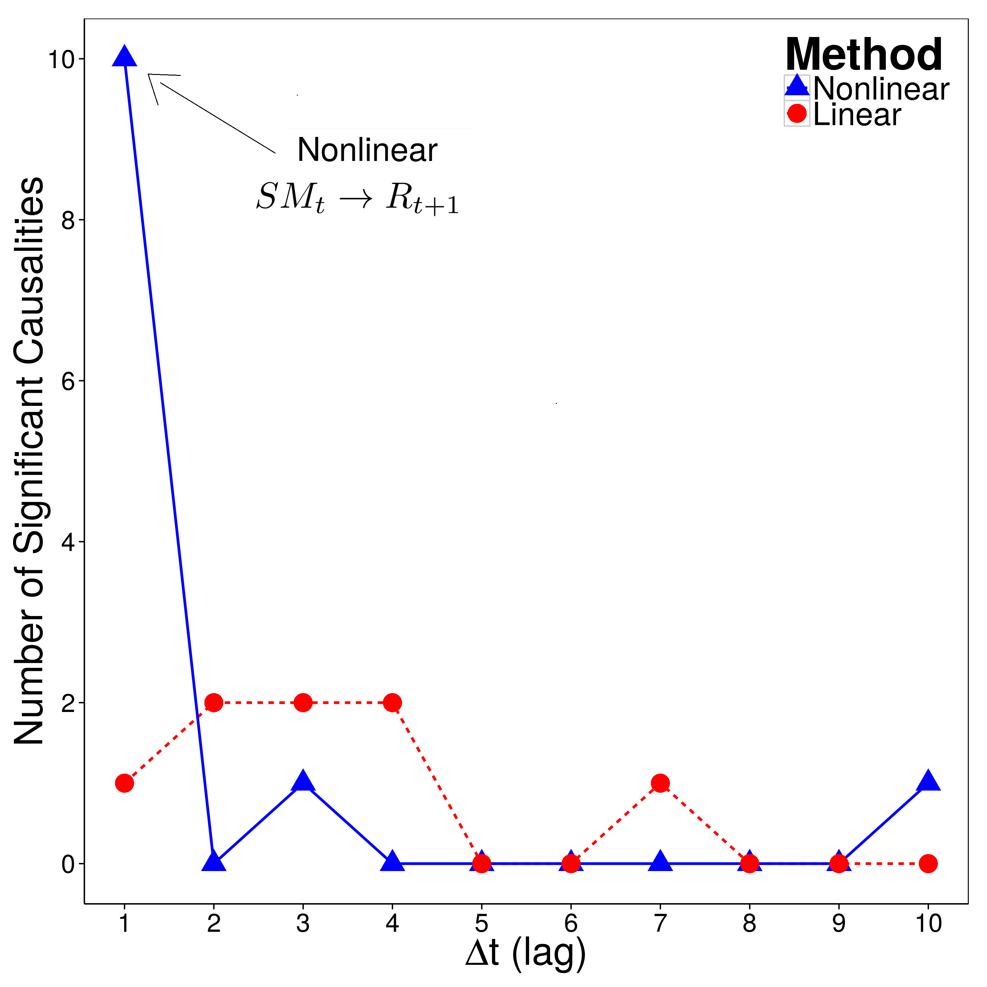
Figure 3: Social media causality on stock’s return is mostly nonlinear in the next-day period. Figure shows the number of companies with significant causality aggregated by lag. Causality between social media and next-day stocks’ returns presents a stunning difference between linear and nonlinear cases. Nonlinear analysis identify much higher causality in the first lag. Hence, linear-constraints may be neglecting social media causality over stocks’ returns, especially in the next-day period. Further lags present a lower number of significant causalities in both methods. p-values are adjusted with a Bonferroni correction to reduce the probability of a Type I (false positive) error due to multiple hypotheses testing. Significance is given at p-value $<0.05$.

Fig. 2 shows the significant causality links between social media and stocks’ returns considering both cases: nonlinear (TE) and linear G-causality . Linear analysis discovers only three stocks with significant causality: INTEL CORP., NIKE INC. and WALT DISNEY CO. Nonlinear analysis discovers that several other stocks have significant causality. In addition to the 3 stocks identified with significant linear causality, other 8 stocks present purely nonlinear causality.

In Fig. 3, we show the number of stocks with significant causality aggregated by lag of interaction. The causality between social media and next-day stocks’ returns presents a stunning difference between linear and nonlinear cases. From linear G-causality one would say that there is significant causality between social media and next-day stocks’ movements for one stock only. Conversely, nonlinear measures indicated that 10 companies have significant causality in this direction. Higher delays show a drop on this number. These results suggest that linear-constraints are neglecting social media causality over stocks’ returns especially in the next-day period or in the short-term.

The low level of causality obtained under linear constraints is inline with results from similar studies in the literature, where it was found that stocks’ returns show weak causality links [6, 29] and social media sentiment analytics, at least when taken alone, have very small or no predictive power [26] and do not have significant lead-time information about stock’s movements for the majority of the stocks [24]. Contrariwise, results from the nonlinear analyses unveiled a much higher level of causality indicating that linear constraints may be neglecting the relationship between social media and stock markets.

Table 1: Nonlinearities found are non-trivial. Test for linear adequacy for commonly used function forms in the relationship between social media and stocks’ returns. Test for misspecification is performed with the BDS test. $x$ represents the standard linear regression of returns on the social media time series. $\nabla x$ and $\nabla^{2}x$ are, respectively, the first and second differencing taken in both time series. $f(x,vol)$ represents a regression of returns on social media controlled by the stocks’ returns daily volatility. In the log-transformation we apply the function $\log(1+x)$ in both time series. The module $|x|$ is applied in the returns time-series which is then regressed over the original social media data. GARCH(1,1) and ARIMA(1,1,1) transformations were applied on returns, then we regressed the resulting residuals on the original social media time series. See Section 6.3 for the description of the functional forms used.

Ticker	$x$	$\nabla x$	$\nabla^{2}x$	$f(x,vol)$	$\log(1+x)$	$|x|$	GARCH(1,1)	ARIMA(1,1,1)
CSCO	$\circ$		$\circ$	$\circ$	$\circ$	$\bullet$	$\circ$	$\circ$
MSFT	$\circ$			$\circ$	$\circ$	$\bullet$	$\circ$	$\circ$
AXP	$\circ$		$\circ$	$\circ$	$\circ$	$\circ$	$\circ$	$\circ$
JPM	$\circ$		$\circ$	$\circ$	$\circ$	$\bullet$	$\circ$	$\circ$
IBM	$\circ$		$\circ$	$\circ$	$\circ$		$\circ$
V			$\circ$
JNJ
AAPL
$\circ$ : Not misspecified; $\bullet$ : Not misspecified and with significant G-causality.

For the companies identified with nonlinear causality, we tested whether common functional forms and transformations used in the literature can explain the nonlinearities. We checked model adequacy and causality significance for various functional forms listed in Table 1, where the results are also reported. The original linear functional form is adequate for 5 companies but can not explain the nonlinear causality. Second-order differencing makes a linear functional adequate for the company VISA, but turns Microsoft as misspecified. GARCH and ARIMA filtering were applied in a tentative to separate signal from noise and to linearize the original time series. Nonetheless, significant causality was not observed. Other functional forms performed no better than the original linear specification a part from the absolute value transformation. It is indeed known that social media and news analytics predict absolute changes in market prices [24, 6] better than stock’s returns. This functional form is a proxy for stock returns volatility and therefore it has higher predictability than stock returns. Yet, half of the companies still had an unexplained nonlinear causality.

It is clear from the results obtained that the nonlinearities found can not be fully explained by returns’ volatility neither by naive transformations often employed in related studies. This indicates that the nonlinear causality is nontrivial and that there is forecastable structure that can not be explained by commonly-used functional forms. Therefore, the impact of social media on market prices may be higher than currently reported in related studies, because commonly-used functional forms are hiding significant causality, that are here reveled instead with a nonparametric analysis.

4 Quantifying the Direction of Information Flow

Transfer-entropy is an asymmetric measure, i.e., $T_{X\rightarrow Y}\neq T_{Y\rightarrow X}$, and thus allows the quantification of directional coupling between systems. The Net Information Flow is defined as $\widehat{TE}_{X\rightarrow Y}=TE_{X\rightarrow Y}-TE_{Y\rightarrow X}$. One can interpret this quantity as a measure of dominant direction of information flow, i.e., a positive result indicates a dominant information flow from $X$ to $Y$ compared to the other direction or, similarly, it indicates which system provides more predictive information about the other system [45].

TE has an intuitive interpretation under the notion of G-causality in the sense that social media may cause (future) stocks’ returns only when it provides more information to stocks’ returns than past stocks’ returns themselves. In fact, Barnett et al. (2009) [46] showed that linear G-causality and Transfer Entropy are equivalent for Gaussian variables. This result provides a direct mapping between the information-theoretic framework and the linear VAR approach of G-causality. Hence, it is possible to estimate TE both in its general form and with its equivalent form for linear G-causality. The former case is a nonparametric approach that is able to capture possible nonlinear coupling that are likely to be neglected in the latter case.

We can therefore quantify the Net Information Flow from social media to stocks’ returns using both nonlinear and linear frameworks. We investigated which direction of coupling is the strongest and to what extent the consideration of nonlinear dynamics affects the results compared to a linear-constrained analysis. Fig. 4 A) shows the results for the linear case. We observe an asymmetry of information, i.e., the systems are not coupled with the same amount of information flow in both directions. The stocks are clearly divided in two groups of approximately same sizes. One group shows stocks with positive net information flow, indicating that social media provides more predictive information about the stock market than the opposite. A second group of stocks indicates the opposite, i.e., information flows more from stocks’ returns to social media than in the other direction. In both cases, the absolute value of net information flow decreases with lag.

Surprisingly, the consideration of nonlinear dynamics unveils a much different scenario. Fig 4 B) shows the results of the same analysis without linear constraints. The net information flow becomes positive for all stocks analyzed. This result suggests that social media is the dominant information source indicating that the information provided by social media contributes more to the description of stock markets dynamics than the opposite.

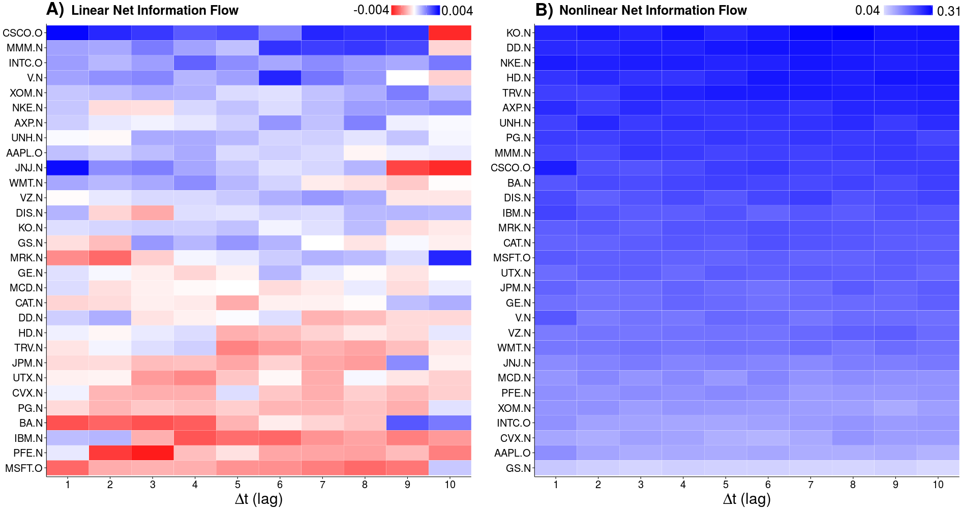
Figure 4: Evidence that linear constraints change to a great extent the direction of Information Flow between social media and stock market. Figure shows the Net Information Flow from social media to stocks’ returns: $\widehat{TE}_{SM\rightarrow R}=TE_{SM\rightarrow R}-TE_{R\rightarrow SM}$. In A), Net Information Flow is estimated with linear constraints. Positive values indicate that $TE_{SM\rightarrow R}>TE_{R\rightarrow SM}$, this is an evidence that information flows from social media to stock returns. Contrariwise, negative values indicate that stock market provide more information about social media movements than the opposite. In B), estimation of Net Information Flow considers nonlinear dynamics. All companies indicate a positive information flow from social media to stocks’ returns. This indicate that, when nonlinear dynamics are considered, the information flows predominantly from social media to stock market. We observe a change of direction of information flow in about half of the companies, compared to the same analysis with linear constraints. Figure shows the stocks ranked by total Net Information Flow considering all lags, i.e., $\sum_{\Delta t=1}^{10}{\widehat{TE}_{SM\rightarrow R}}$.

5 Summary

The present study has revealed that social media has a significant nonlinear impact on stocks’ returns.

We analyzed an extensive data set of social media analytics related to stocks components of the DJIA index. Nonparametric tests for nonlinear specification and causality indicated three major empirical findings:

1. The consideration of nonlinear dynamics increased the number of stocks with relevant social media signal from 1/10, in the linear case, to more than 1/3 indicating that social media significant causality on stocks’ returns are purely nonlinear in most cases;
   

2. The nonlinearities found were nontrivial and could not be explained by common functional forms used in the literature. This indicates that the impact of social media on stocks’ returns may be higher than currently reported in related studies;
   

3. Nonparametric analysis indicated that social media dominates the directional coupling with stock market; an effect not observable within linear constraints.

We suggest that social media explanatory power on stock markets may be intensified if nonlinear dynamics are considered. In this respect, we provided strong evidence that supports the use of social media as a valuable source of information about the stock market.

From a methodological point of view, results indicate that a nonparametric approach is highly preferable for the investigation of causal relationships between sociotechnical and financial systems.

6 Methods

6.1 BDS Test for Linear Misspecification

When applied to the residuals of a linear model, the BDS test [40] is a powerful test to detect nonlinearity [41]. Let $\epsilon_{t}=(\epsilon_{t=1},\ldots,\epsilon_{t=n})$ be the residuals of the linear fitted model and define its $m$-embedding as $\epsilon_{t}^{m}=(\epsilon_{t},\epsilon_{t-1},\ldots,\epsilon_{t-m+1})$. The $m$-embedding correlation integral is given by

$$C_{m,n}(\Delta\epsilon)=\frac{2}{k(k-1)}\sum_{s=1}^{t}{\sum_{t=s}^{n}{\chi(\|\epsilon_{s}^{m}-\epsilon_{t}^{m}\|,\Delta\epsilon)}},$$ (1)

and

$$C_{m}(\Delta\epsilon)=\lim_{n\to\infty}C_{m,n}(\Delta\epsilon),$$ (2)

where $\chi$ is an indicator function with $\chi(\|\epsilon_{s}^{m}-\epsilon_{t}^{m}\|,\Delta\epsilon)=1$ if $\|\epsilon_{s}^{m}-\epsilon_{t}^{m}\|<\Delta\epsilon$ and zero, otherwise. The null hypothesis of the BDS test assumes that $\epsilon_{t}$ is iid. In this case,

$$C_{m}(\Delta\epsilon)=C_{1}(\Delta\epsilon)^{m}.$$ (3)

The BDS statistic is a measure of the extent that this relation holds in the data. It is given by:

$$V_{m}(\Delta\epsilon)=\sqrt{n}\frac{C_{m}(\Delta\epsilon)-C_{1}(\Delta\epsilon)^{m}}{\sigma_{m}(\Delta\epsilon)},$$ (4)

where $\sigma_{m}(\Delta\epsilon)$ can be estimated as described in [40]. The null hypothesis of the BDS test indicates that the model tested is not misspecified and it is rejected at 5% significance level if $\|V_{m}(\Delta\epsilon)\|>1.96$.

$\Delta\epsilon$ is commonly set as a factor of the variance ($\sigma_{\epsilon}$) of $\epsilon$. We report results for $\Delta\epsilon=\sigma_{\epsilon}/2$ and the embedding dimension $m=2$. We also performed tests for $\Delta\epsilon=\sigma_{\epsilon}$ and $m=3$ with no significant differences in the results.

6.2 Linear G-causality

Consider the linear vector-autoregressive (VAR) equations:

$$R(t) ={\alpha}+\sum^{k}_{\Delta t=1}{{\beta}_{\Delta t}R(t-\Delta t)}+\epsilon_{t},$$ (5)

$$R(t) =\widehat{\alpha}+\sum^{k}_{\Delta t=1}{{\widehat{\beta}}_{\Delta t}R(t-\Delta t)}+\sum^{k}_{\Delta t=1}{{\widehat{\gamma}}_{\Delta t}SM(t-\Delta t)}+\widehat{\epsilon}_{t},$$ (6)

we test whether $SM$ G-causes $R$ by comparing the errors in the prediction of $R$ in the restricted and unrestricted regression models in Eq. (5) and Eq. (12), respectively. Significance estimation is performed via analysis of variance. We indicated a significant causality if there is significant causality in at least one of the lags tested. We adjusted the p-values with a Bonferroni correction to control for multiple hypotheses testing.

6.3 Functional Forms Tested

Functional forms referenced in Table 1 were used as following.

6.3.1 Differencing: $\nabla x$.

The first differencing is taken in both social media and returns time series.

$$\nabla(R(t),1) =\widehat{\alpha}+\sum^{k}_{\Delta t=1}{{\widehat{\beta}}_{\Delta t}\nabla(R(t-\Delta t),1)}+\sum^{k}_{\Delta t=1}{{\widehat{\gamma}}_{\Delta t}\nabla(SM(t-\Delta t),1)}+\widehat{\epsilon}_{t}.$$ (7)

The second differencing $\nabla^{2}x$ was tested in analogous way.

6.3.2 $f(x,vol)$.

Represents a regression of returns on social media controlled by the stocks’ returns daily volatility.

$$R(t) =\widehat{\alpha}+\sum^{k}_{\Delta t=1}{{\widehat{\beta}}_{\Delta t}R(t-\Delta t)}+\sum^{k}_{\Delta t=1}{{\widehat{\gamma}}_{\Delta t}SM(t-\Delta t)}+\sum^{k}_{\Delta t=1}{{\widehat{\theta}}_{\Delta t}vol(t-\Delta t)}+\widehat{\epsilon}_{t},$$ (8)

where we consider

$$vol(t)=2\frac{P_{high}(t)-P_{low}(t)}{P_{high}(t)+P_{low}(t)}$$ (9)

as an approximation of the daily returns volatility. $P_{high}$ and $P_{low}$ are the highest and lowest intraday price value, respectively.

6.3.3 Log-transformation: $log(x+1)$.

$$\log(R(t)+1) =\widehat{\alpha}+\sum^{k}_{\Delta t=1}{{\widehat{\beta}}_{\Delta t}\log(R(t-\Delta t)+1)}+\sum^{k}_{\Delta t=1}{{\widehat{\gamma}}_{\Delta t}\log(SM(t-\Delta t)+1)}+\widehat{\epsilon}_{t}.$$ (10)

6.3.4 Absolute value: $|x|$.

$$|R(t)| =\widehat{\alpha}+\sum^{k}_{\Delta t=1}{{\widehat{\beta}}_{\Delta t}|R(t-\Delta t)|}+\sum^{k}_{\Delta t=1}{{\widehat{\gamma}}_{\Delta t}SM(t-\Delta t)}+\widehat{\epsilon}_{t}.$$ (11)

6.3.5 GARCH(1,1).

A GARCH filtering was applied in the original returns time series as follows:

$$R(t) =\alpha+\sum^{p}_{\Delta t=1}{{\beta}_{\Delta t}R(t-\Delta t)}+\sum^{q}_{\Delta t=1}{{\gamma}_{\Delta t}\epsilon_{t-\Delta t}},$$ (12)

with $p=1$, $q=1$ and

$$\epsilon_{t}\sim N(0,R(t)).$$ (13)

The resulting residuals $\epsilon_{t}$ were then used instead of the original returns time series $R(t)$.

6.3.6 ARIMA(1,1,1).

ARIMA filtering was applied in the original returns time series as follows:

$$R(t) =R(t-1)+\alpha(SM(t-1)-SM(t-2))+\beta\epsilon_{t-1}.$$ (14)

The resulting residuals $\epsilon_{t}$ were then used instead of the original returns time series $R(t)$.

6.4 Nonparametric G-Causality: Transfer Entropy

Transfer Entropy (TE) was estimated as a sum of Shannon entropies:

$$TE\left(X\rightarrow Y\right)=H\left(Y^{P},X^{P}\right)-H\left(Y^{F},Y^{P},X^{P}\right)+H\left(Y^{F},Y^{P}\right)-H\left(Y^{P}\right),$$ (15)

where $Y^{F}$ is a forward time-shifted version of $Y$ at lag $\Delta t$ relatively to the contemporaneous time-series $X^{P}$ and $Y^{P}$. We reject the null hypothesis of causality if the Transfer Entropy from social media to stocks’ returns is significant. To remain in a nonparametric framework, the statistical significance of TE was performed using surrogate data. In that way, 400 replicates of $TE(X_{Shuffled}\rightarrow Y)$ were estimated, where $X_{Shuffled}$ is a random permutation of $X$ relatively to $Y$. We computed the randomized Transfer Entropy at each permutation for each time-shift ($\Delta t$) from 1 to 10 days. We then calculated the frequency at which the observed Transfer Entropy was equal or more extreme than the randomized Transfer Entropy of the surrogate data. Statistical significance was given at p-value $<0.05$. p-values were also Bonferroni corrected.

The estimation of the empirical probability density distribution, required for the entropy estimation, was performed using a Kernel Density Estimation (KDE) method, which has several advantages over the commonly used Histogram based methods (see SI.B.2).

6.5 Net Information Flow

The Net Information Flow from social media to the stock market is defined as: $\widehat{TE}_{SM\rightarrow R}=TE_{SM\rightarrow R}-TE_{R\rightarrow SM}$. For the nonlinear case, transfer entropy was computed as defined in the previous Section 6.4. Instead, to estimate a linear version of Net Information Flow, we compute Transfer Entropy for the linear case based on the work of [46]. This work provides a direct mapping between Transfer Entropy and the linear G-causality implemented in the standard VAR framework. The authors showed that Transfer Entropy and linear G-causality are equivalent for Gaussian variables.

Particularly, assuming the standard measure of linear G-causality for the bivariate case as

$$GC_{X\rightarrow Y}=\log\left(\frac{var(\epsilon_{t})}{var(\widehat{\epsilon}_{t})}\right).$$ (16)

[46] shows that:

$$GC_{X\rightarrow Y}=2TE_{X\rightarrow Y},$$ (17)

if all processes ($X$ and $Y$) are jointly Gaussian.

See Supporting Information for the Material (SI.A) used and further details in the Transfer Entropy estimation SI.B.

Supporting Information

SI.A Material

SI.A.1 List of Companies Analyzed

The name of the investigated stocks with respective Reuters Instrument Codes (RIC) follow: INTEL CORP. (INTC.O), VISA INC. (V.N), NIKE INC. (NKE.N), E.I. DUPONT DE NEMOURS & CO. (DD.N), JPMORGAN CHASE & CO. (JPM.N), BOEING CO. (BA.N), MERCK & CO. INC. (MRK.N), PFIZER INC. (PFE.N), MICROSOFT CORP. (MSFT.O), COCA-COLA CO. (KO.N), GOLDMAN SACHS GROUP INC. (GS.N), MCDONALD’S CORP. (MCD.N), GENERAL ELECTRIC CO. (GE.N), 3M CO. (MMM.N), UNITED TECHNOLOGIES CORP. (UTX.N), VERIZON COMMUNICATIONS INC. (VZ.N), CISCO SYSTEMS INC. (CSCO.O), HOME DEPOT INC. (HD.N), INTERNATIONAL BUSINESS MACHINES CORP. (IBM.N), AMERICAN EXPRESS CO. (AXP.N), PROCTER & GAMBLE CO. (PG.N), APPLE INC. (AAPL.O), UNITEDHEALTH GROUP INC. (UNH.N), CATERPILLAR INC. (CAT.N), EXXON MOBIL CORP. (XOM.N), JOHNSON & JOHNSON (JNJ.N), WAL-MART STORES INC. (WMT.N), WALT DISNEY CO. (DIS.N), CHEVRON CORP. (CVX.N) and THE TRAVELERS COMPANIES INC. (TRV.N).

SI.A.2 Twitter Data Analytics

Twitter data analytics were provided by PsychSignal.com [37]. The data are comprised of volume measures and sentiment analytics. Twitter messages are classified in two dimensions according to their likelihood of bullishness and bearishness towards a company. A company is defined to be related to a given message if its ticker is mentioned. The data set are based on English language content and it is agnostic to the country source of the Twitter message. The information is aggregated in a daily fashion and it is composed of the following variables:

• symbol: the stock symbol (ticker) for which the sentiment data refer to;
  

• timestamp_utc: date and time of the analyzed data in UTC format;
  

• bull_scored_messages: this indicator is the total count of bullish sentiment messages;
  

• bear_scored_messages: this indicator is the total count of bearish sentiment messages.

Some messages may be classified as “neutral” or at least not having relevant bullish or bearish tones. Those types of messages do not affect the bull_scored_messages and bear_scored_messages scores. It is also possible that no messages cite a company in a given day. In that case, the scores are zero.

Table SI.A shows an example of the Twitter sentiment analytics for the company APPLE INC. Table SI.B shows a summary description of the selected companies with the number of bearish/bullish Twitter messages identified in the period.

Table SI.A: Sample of Twitter Sentiment Analytics for the company APPLE INC. Twitter messages mentioning a company’s ticker (symbol) are classified according to their bullish/bearish tones. The table shows a sample of the daily total of bearish and bullish messages classified for the company APPLE INC.

timestamp_utc	symbol	bull_scored_messages	bear_scored_messages
2015-06-19	AAPL.O	216	55
2015-06-20	AAPL.O	66	25
2015-06-21	AAPL.O	90	24
2015-06-22	AAPL.O	241	75
2015-06-23	AAPL.O	208	75
2015-06-24	AAPL.O	561	211
2015-06-25	AAPL.O	286	107
2015-06-26	AAPL.O	192	82
2015-06-27	AAPL.O	145	12
2015-06-28	AAPL.O	216	69

Table SI.B: Summary table of selected companies. DJIA stocks along with their total and daily mean number of Bearish and Bullish tweets during the period from March 31, 2012 to March 31, 2014. The number of total messages processed include not only messages labeled as bullish and bearish but also neutral messages.

	Bullish messages		Bearish messages
Ticker	Total	Daily mean	Total	Daily mean	Total Messages
AAPL	151143	279.89	95819	177.443	800638
MSFT	16730	30.98	7062	13.078	139343
JPM	11259	20.85	6090	11.278	82265
GS	13971	25.87	8023	14.857	75578
IBM	7387	13.68	4284	7.933	53547
INTC	6808	12.61	3199	5.924	47653
GE	4888	9.05	1522	2.819	41271
CSCO	5919	10.96	2535	4.694	39665
WMT	4702	8.71	2438	4.515	39607
XOM	4495	8.32	1780	3.296	33194
CAT	5854	10.84	4035	7.472	31911
VZ	4101	7.59	1651	3.057	30936
BA	4432	8.21	1693	3.135	30421
JNJ	3575	6.62	1345	2.491	28392
MCD	3750	6.94	2157	3.994	28059
KO	3786	7.01	1385	2.565	26331
DIS	4170	7.72	1282	2.374	25863
PFE	3131	5.80	1091	2.020	24817
V	4436	8.21	1726	3.196	24118
CVX	2696	4.99	986	1.826	21322
NKE	3549	6.57	1461	2.706	20941
MRK	2623	4.86	929	1.720	20708
PG	2382	4.41	968	1.793	20226
HD	3262	6.04	1221	2.261	17550
MMM	1399	2.59	465	0.861	12382
AXP	1740	3.22	674	1.248	12072
UTX	1363	2.55	369	0.690	11255
DD	1498	2.78	559	1.037	10746
UNH	1348	2.50	532	0.987	9196
TRV	798	1.53	316	0.604	7990
TOTAL	287195	-	157597	-	1767997

SI.B Transfer-Entropy Estimation

SI.B.1 Definitions of information theoretic measures

Let $X$ be a random variable and $P_{X}(x)$ its probability density function (pdf). The entropy $H(X)$ is a measure of uncertainty of $X$, and is defined in the discrete case, as:

$$H(X)=-\sum_{x\in X}{P_{X}(x)\log{P_{X}(x)}}.$$ (18)

If the $\log$ is taken to base two, then the unit of $H$ is the bit (binary digit). Here, we employ the natural logarithm which implies the unit in nat (natural unit of information).

Given a coupled system $(X,Y)$, where $P_{Y}(y)$ is the pdf of the random variable $Y$ and $P_{X,Y}$ the joint pdf between $X$ and $Y$, the joint entropy is given by:

$$H(X,Y)=-\sum_{x\in X}{\sum_{y\in Y}{P_{X,Y}(x,y)\log{P_{X,Y}(x,y)}}}.$$ (19)

The conditional entropy is defined by:

$$H\left(Y\middle|X\right)=H(X,Y)-H(X).$$ (20)

We can interpret $H\left(Y\middle|X\right)$ as the uncertainty of $Y$ given a realization of $X$.

Transfer Entropy can be defined as a difference between conditional entropies:

$$TE\left(X\rightarrow Y\right)=TE\left(X^{P},Y^{F}\middle|Y^{P}\right)=H\left(Y^{F}\middle|Y^{P}\right)-H\left(Y^{F}\middle|X^{P},Y^{P}\right),$$ (21)

which can be rewritten as a sum of Shannon entropies:

$$TE\left(X\rightarrow Y\right)=H\left(Y^{P},X^{P}\right)-H\left(Y^{F},Y^{P},X^{P}\right)+H\left(Y^{F},Y^{P}\right)-H\left(Y^{P}\right),$$ (22)

where $Y^{F}$ is a forward time-shifted version of $Y$ at lag $\Delta t$ relatively to the contemporaneous time-series $X^{P}$ and $Y^{P}$.

SI.B.2 Kernel Density Estimation

In the entropy computation, the empirical probability distribution must be estimated. Histogram based methods and kernel density estimations are the two main methods for that. Histogram-based is the simplest and most used nonparametric density estimator. Nonetheless, it yields density estimates that have discontinuities and vary significantly depending on the bin’s size choice.

Also known as Parzen-Rosenblatt window method, the kernel density estimation (KDE) approach approximates the density function at a point $x$ using neighboring observations. However, instead of building up the estimate according to bin edges as in histograms, the KDE method uses each point of estimation $x$ as the center of a bin of width $2h$ and weight it according to a kernel function. Thereby, the kernel estimate of the probability density function $f(x)$ is defined as

$$\hat{f}=\frac{1}{nh}\sum_{x^{\prime}\in X}{K\left(\frac{x-x^{\prime}}{h}\right)}.$$ (23)

A usual choice for the kernel $K$, which we use here, is the (Gaussian) radial basis function:

$$K(x)=\frac{1}{\sqrt{2\pi}}\exp^{-\frac{1}{2}x^{2}}.$$ (24)

The problem of selecting the bandwidth $h$ in equation (23) is crucial in the density estimation. A large $h$ will over-smooth the estimated density and mask the structure of the data. On the other hand, a small bandwidth will reduce the bias of the density estimate at the expense of a larger variance in the estimates. If we assume that the true distribution is Gaussian and we use a Gaussian kernel, the optimal value of $h$ that minimizes the mean integrated squared error (MISE) is

$$h^{*}=1.06\sigma N^{-1/5},$$

where $N$ is the total number of points and $\sigma$ can be estimated as the sample standard deviation. This bandwidth estimation is often called Gaussian approximation or Silverman’s rule of thumb for kernel density estimation [47]. This is the most common used method and it is here employed. Other common methods are given by Sheather and Jones [48] and Scott [49].

SI.C Results of the BDS and causality tests

Table SI.C: Results of the BDS test. Significance of the null hypothesis of linear specification between Social Media and stocks’ returns. Social media bullishness is taken as independent variable with stocks’ returns as outcome variable. p-values higher than 0.05 are evidence of misspecification of the linear functional form indicating a nonlinearly neglected relationship. Lags of up to 10 days were tested. p-value $<0.05$: *; p-value $<0.01$: **.

	Lags $\Delta t$ for: $R_{t}=\sum_{i=1}^{\Delta t}\alpha_{i}R_{t-\Delta t}+\sum_{i=1}^{\Delta t}\beta_{i}SM_{t-\Delta t}$
Ticker	1	2	3	4	5	6	7	8	9	10
MMM.N	0.928	0.780	0.768	0.999	0.668	0.747	0.739	0.362	0.389	0.676
AXP.N	0.906	0.987	0.503	0.795	0.734	0.432	0.737	0.336	0.197	0.132
AAPL.O	0.015*	0.023*	0.028*	0.018*	0.018*	0.008**	0.007**	0.002**	0.003**	0.009**
BA.N	0.834	0.700	0.591	0.239	0.187	0.363	0.287	0.345	0.187	0.213
CAT.N	0.001**	0.002**	0.001**	0.000**	0.000**	0.000**	0.000**	0.001**	0.004**	0.002**
CVX.N	0.113	0.073	0.202	0.330	0.150	0.151	0.389	0.268	0.275	0.439
CSCO.O	0.404	0.443	0.500	0.463	0.436	0.814	0.883	0.639	0.597	0.590
KO.N	0.544	0.905	0.712	0.864	0.451	0.734	0.653	0.702	0.471	0.793
DD.N	0.523	0.373	0.170	0.295	0.759	0.254	0.311	0.199	0.204	0.169
XOM.N	0.986	0.871	0.504	0.382	0.502	0.704	0.635	0.648	0.178	0.202
GE.N	0.055	0.016*	0.017*	0.112	0.117	0.129	0.103	0.098	0.101	0.101
GS.N	0.077	0.010**	0.041*	0.021*	0.028*	0.068	0.102	0.065	0.079	0.014*
HD.N	0.171	0.092	0.348	0.211	0.079	0.231	0.188	0.034*	0.011*	0.037*
INTC.O	0.888	0.931	0.808	0.880	0.828	0.858	0.735	0.968	0.756	0.825
IBM.N	0.184	0.201	0.121	0.126	0.066	0.216	0.393	0.344	0.263	0.209
JNJ.N	0.000**	0.000**	0.000**	0.000**	0.000**	0.000**	0.000**	0.000**	0.000**	0.000**
JPM.N	0.171	0.133	0.146	0.305	0.401	0.322	0.270	0.304	0.246	0.798
MCD.N	0.837	0.970	0.953	0.944	0.497	0.708	0.768	0.775	0.995	0.988
MRK.N	0.031*	0.026*	0.015*	0.054	0.074	0.134	0.157	0.089	0.126	0.210
MSFT.O	0.138	0.079	0.129	0.031*	0.009**	0.074	0.066	0.080	0.201	0.136
NKE.N	0.220	0.126	0.124	0.158	0.055	0.146	0.033*	0.061	0.035*	0.023*
PFE.N	0.606	0.601	0.599	0.573	0.346	0.405	0.526	0.777	0.651	0.838
PG.N	0.005**	0.010*	0.012*	0.016*	0.054	0.052	0.015*	0.017*	0.022*	0.017*
TRV.N	0.000**	0.000**	0.000**	0.000**	0.000**	0.002**	0.003**	0.000**	0.000**	0.000**
UNH.N	0.007**	0.014*	0.036*	0.016*	0.019*	0.013*	0.006**	0.039*	0.016*	0.011*
UTX.N	0.176	0.204	0.256	0.577	0.084	0.079	0.185	0.254	0.725	0.585
VZ.N	0.001**	0.000**	0.000**	0.001**	0.002**	0.000**	0.001**	0.027*	0.000**	0.000**
V.N	0.001**	0.000**	0.000**	0.000**	0.003**	0.022*	0.049*	0.017*	0.023*	0.023*
WMT.N	0.200	0.364	0.525	0.937	0.839	0.646	0.719	0.976	0.946	0.753
DIS.N	0.294	0.310	0.217	0.173	0.421	0.285	0.174	0.179	0.270	0.432

Table SI.D: Significance for nonlinear causality tests. Lags of up to 10 days were tested in both directions of causality: social media causing returns $SM\rightarrow R$ and the opposite, returns causing social media $R\rightarrow SM$. p-value $<0.05$: *; p-value $<0.01$: **.

	Lagged $R\rightarrow SM$										Lagged $SM\rightarrow R$
Ticker	1	2	3	4	5	6	7	8	9	10	1	2	3	4	5	6	7	8	9	10
MMM.N	0.257	0.248	0.970	0.530	0.198	0.838	0.655	0.767	0.505	0.615	0.410	0.765	0.755	0.570	0.568	0.973	0.980	0.797	0.825	0.945
AXP.N	0.145	0.275	0.480	0.002**	0.157	0.310	0.380	0.475	0.328	0.142	0.000**	0.297	0.282	0.160	0.407	0.098	0.440	0.152	0.405	0.118
AAPL.O	0.440	0.995	0.710	0.512	0.912	0.988	0.980	0.897	0.615	0.990	0.000**	0.745	0.590	0.140	0.682	0.585	0.782	0.715	0.095	0.975
BA.N	0.090	0.475	0.110	0.110	0.718	0.160	0.062	0.345	0.050	0.150	0.287	0.297	0.262	0.070	0.103	0.123	0.095	0.545	0.510	0.130
CAT.N	0.265	0.562	0.162	0.607	0.170	0.787	0.623	0.235	0.480	0.435	0.055	0.540	0.245	0.228	0.297	0.025*	0.157	0.035*	0.485	0.348
CVX.N	0.422	0.500	0.710	0.667	0.130	0.040*	0.073	0.955	0.745	0.585	0.270	0.973	0.218	0.382	0.478	0.932	0.528	0.343	0.500	0.330
CSCO.O	0.083	0.220	0.047*	0.340	0.797	0.605	0.703	0.355	0.325	0.818	0.000**	0.655	0.488	0.528	0.292	0.218	0.500	0.785	0.537	0.645
KO.N	0.160	0.377	0.095	0.617	0.010*	0.103	0.270	0.405	0.020*	0.073	0.193	0.297	0.365	0.295	0.568	0.162	0.005**	0.015*	0.235	0.575
DD.N	0.330	0.098	0.055	0.047*	0.758	0.620	0.752	0.722	0.330	0.542	0.535	0.792	0.275	0.295	0.323	0.147	0.478	0.705	0.760	0.377
XOM.N	0.955	0.677	0.580	0.738	0.838	0.735	0.375	0.593	0.002**	0.375	0.100	0.015*	0.532	0.105	0.662	0.742	0.333	0.722	0.720	0.575
GE.N	0.698	0.190	0.540	0.262	0.415	0.292	0.660	0.610	0.415	0.377	0.182	0.443	0.633	0.032*	0.260	0.613	0.522	0.277	0.080	0.007**
GS.N	0.655	0.350	0.083	0.595	0.175	0.252	0.657	0.245	0.580	0.145	0.353	0.735	0.752	0.520	0.200	0.490	0.885	0.722	0.838	0.867
HD.N	0.345	0.350	0.000**	0.007**	0.080	0.532	0.767	0.490	0.320	0.532	0.495	0.225	0.062	0.200	0.167	0.115	0.392	0.555	0.080	0.177
INTC.O	0.150	0.902	0.290	0.660	0.088	0.463	0.718	0.910	0.550	0.745	0.000**	0.848	0.248	0.818	0.420	0.570	0.443	0.245	0.330	0.310
IBM.N	0.037*	0.458	0.248	0.390	0.672	0.205	0.318	0.505	0.463	0.800	0.000**	0.017*	0.333	0.722	0.198	0.637	0.088	0.607	0.052	0.498
JNJ.N	0.490	0.292	0.275	0.677	0.703	0.282	0.402	0.930	0.508	0.287	0.108	0.015*	0.000**	0.380	0.020*	0.125	0.562	0.290	0.137	0.015*
JPM.N	0.040*	0.057	0.060	0.353	0.035*	0.017*	0.057	0.262	0.330	0.125	0.000**	0.027*	0.030*	0.010*	0.010*	0.145	0.050	0.012*	0.123	0.000**
MCD.N	0.088	0.943	0.287	0.885	0.037*	0.680	0.287	0.597	0.848	0.780	0.180	0.502	0.740	0.552	0.565	0.090	0.657	0.392	0.840	0.838
MRK.N	0.220	0.675	0.345	0.475	0.595	0.767	0.445	0.132	0.213	0.277	0.307	0.593	0.835	0.518	0.568	0.502	0.532	0.190	0.542	0.653
MSFT.O	0.040*	0.732	0.690	0.200	0.093	0.118	0.162	0.270	0.573	0.390	0.000**	0.468	0.568	0.580	0.302	0.115	0.498	0.407	0.323	0.815
NKE.N	0.032*	0.287	0.435	0.145	0.152	0.020*	0.243	0.483	0.235	0.147	0.000**	0.167	0.390	0.167	0.627	0.110	0.225	0.440	0.593	0.358
PFE.N	0.113	0.057	0.762	0.438	0.758	0.167	0.020*	0.762	0.667	0.680	0.017*	0.267	0.290	0.307	0.198	0.110	0.570	0.993	0.873	0.643
PG.N	0.797	0.387	0.838	0.175	0.645	0.267	0.340	0.118	0.453	0.103	0.215	0.277	0.167	0.297	0.550	0.427	0.200	0.375	0.830	0.988
TRV.N	0.415	0.040*	0.695	0.330	0.177	0.045*	0.427	0.083	0.395	0.395	0.380	0.238	0.270	0.377	0.115	0.115	0.085	0.132	0.255	0.545
UNH.N	0.022*	0.035*	0.002**	0.093	0.037*	0.090	0.015*	0.170	0.123	0.245	0.022*	0.030*	0.050	0.050	0.243	0.213	0.100	0.165	0.402	0.152
UTX.N	0.432	0.528	0.560	0.218	0.280	0.867	0.855	0.228	0.480	0.703	0.713	0.302	0.275	0.848	0.037*	0.682	0.407	0.050	0.325	0.805
VZ.N	0.098	0.650	0.052	0.090	0.108	0.135	0.463	0.748	0.127	0.600	0.090	0.758	0.535	0.782	0.300	0.630	0.198	0.027*	0.007**	0.373
V.N	0.400	0.645	0.782	0.353	0.742	0.603	0.218	0.613	0.818	0.915	0.000**	0.970	0.780	0.400	0.130	0.368	0.802	0.483	0.715	0.905
WMT.N	0.458	0.762	0.787	0.493	0.693	0.262	0.848	0.365	0.365	0.272	0.115	0.382	0.150	0.302	0.267	0.195	0.203	0.445	0.147	0.438
DIS.N	0.510	0.083	0.448	0.630	0.090	0.640	0.985	0.147	0.262	0.795	0.002**	0.742	0.902	0.550	0.762	0.532	0.130	0.935	0.627	0.665

Table SI.E: Significance for linear causality tests. Lags of up to 10 days were tested in both directions of causality: social media causing returns $SM\rightarrow R$ and the opposite, returns causing social media $R\rightarrow SM$. p-value $<0.05$: *; p-value $<0.01$: **.

	Lagged $R\rightarrow SM$										Lagged $SM\rightarrow R$
Ticker	1	2	3	4	5	6	7	8	9	10	1	2	3	4	5	6	7	8	9	10
MMM.N	0.024*	0.080	0.131	0.213	0.260	0.292	0.308	0.180	0.232	0.240	0.063	0.122	0.129	0.175	0.029*	0.058	0.077	0.131	0.165	0.238
AXP.N	0.584	0.687	0.785	0.812	0.905	0.942	0.971	0.987	0.972	0.937	0.671	0.878	0.241	0.341	0.441	0.398	0.425	0.260	0.386	0.158
AAPL.O	0.068	0.029*	0.066	0.084	0.189	0.073	0.173	0.214	0.284	0.355	0.242	0.434	0.607	0.451	0.527	0.028*	0.039*	0.049*	0.035*	0.026*
BA.N	0.554	0.813	0.943	0.982	0.852	0.878	0.809	0.645	0.667	0.613	0.370	0.574	0.615	0.382	0.469	0.518	0.505	0.518	0.646	0.430
CAT.N	0.141	0.240	0.160	0.264	0.269	0.201	0.302	0.231	0.177	0.232	0.967	0.989	0.991	0.995	0.993	0.994	0.967	0.542	0.609	0.687
CVX.N	0.517	0.658	0.778	0.888	0.294	0.364	0.258	0.253	0.314	0.336	0.678	0.919	0.906	0.965	0.941	0.973	0.986	0.991	0.995	0.997
CSCO.O	0.870	0.954	0.985	0.984	0.959	0.942	0.968	0.453	0.548	0.606	0.834	0.886	0.945	0.980	0.982	0.988	0.979	0.991	0.996	0.995
KO.N	0.753	0.562	0.694	0.776	0.477	0.565	0.687	0.658	0.119	0.211	0.149	0.264	0.024*	0.046*	0.084	0.125	0.198	0.009**	0.012*	0.025*
DD.N	0.283	0.390	0.533	0.088	0.165	0.232	0.332	0.323	0.358	0.419	0.457	0.575	0.759	0.660	0.673	0.557	0.647	0.720	0.809	0.831
XOM.N	0.640	0.282	0.393	0.549	0.650	0.702	0.866	0.927	0.153	0.217	0.192	0.266	0.375	0.112	0.089	0.084	0.111	0.069	0.062	0.096
GE.N	0.465	0.327	0.615	0.528	0.574	0.468	0.602	0.685	0.425	0.531	0.719	0.883	0.954	0.745	0.806	0.887	0.735	0.775	0.755	0.625
GS.N	0.516	0.566	0.822	0.829	0.529	0.517	0.651	0.602	0.628	0.517	0.245	0.287	0.493	0.632	0.708	0.725	0.823	0.831	0.836	0.815
HD.N	0.293	0.461	0.012*	0.031*	0.047*	0.087	0.134	0.153	0.204	0.226	0.773	0.971	0.473	0.269	0.315	0.431	0.641	0.414	0.427	0.463
INTC.O	0.040*	0.089	0.130	0.196	0.280	0.352	0.479	0.507	0.329	0.354	0.000**	0.000**	0.002**	0.004**	0.009**	0.019*	0.012*	0.023*	0.037*	0.079
IBM.N	0.612	0.338	0.258	0.364	0.529	0.345	0.285	0.314	0.300	0.208	0.008**	0.032*	0.073	0.163	0.217	0.128	0.164	0.230	0.264	0.323
JNJ.N	0.278	0.306	0.538	0.484	0.388	0.501	0.532	0.657	0.739	0.754	0.085	0.224	0.244	0.425	0.563	0.189	0.203	0.126	0.097	0.147
JPM.N	0.134	0.010**	0.020*	0.042*	0.078	0.092	0.135	0.176	0.245	0.317	0.010*	0.038*	0.053	0.013*	0.041*	0.077	0.070	0.106	0.151	0.104
MCD.N	0.691	0.542	0.806	0.912	0.936	0.727	0.627	0.694	0.683	0.714	0.176	0.350	0.320	0.529	0.304	0.318	0.250	0.443	0.392	0.482
MRK.N	0.893	0.232	0.314	0.417	0.144	0.167	0.198	0.178	0.103	0.062	0.864	0.965	0.990	0.995	0.990	0.772	0.679	0.863	0.918	0.932
MSFT.O	0.245	0.466	0.666	0.616	0.771	0.211	0.225	0.313	0.319	0.411	0.328	0.347	0.451	0.311	0.406	0.124	0.218	0.112	0.173	0.206
NKE.N	0.054	0.043*	0.028*	0.063	0.104	0.147	0.174	0.180	0.232	0.308	0.008**	0.001**	0.002**	0.003**	0.006**	0.013*	0.017*	0.034*	0.038*	0.050
PFE.N	0.827	0.974	0.968	0.974	0.965	0.957	0.968	0.949	0.695	0.700	0.821	0.972	0.789	0.880	0.887	0.896	0.904	0.927	0.932	0.963
PG.N	0.115	0.236	0.235	0.343	0.409	0.475	0.382	0.463	0.599	0.616	0.668	0.476	0.615	0.552	0.527	0.652	0.749	0.766	0.745	0.825
TRV.N	0.097	0.217	0.262	0.192	0.060	0.036*	0.067	0.014*	0.018*	0.029*	0.532	0.787	0.155	0.229	0.341	0.203	0.284	0.213	0.058	0.081
UNH.N	0.038*	0.093	0.139	0.226	0.102	0.151	0.173	0.250	0.277	0.322	0.116	0.279	0.423	0.583	0.668	0.731	0.779	0.790	0.846	0.912
UTX.N	0.700	0.780	0.973	0.988	0.525	0.486	0.432	0.581	0.635	0.566	0.618	0.761	0.249	0.343	0.402	0.507	0.505	0.706	0.347	0.441
VZ.N	0.348	0.454	0.635	0.808	0.740	0.494	0.456	0.564	0.664	0.748	0.231	0.450	0.586	0.702	0.553	0.434	0.424	0.474	0.026*	0.040*
V.N	0.033*	0.059	0.097	0.209	0.245	0.269	0.222	0.062	0.095	0.130	0.242	0.369	0.204	0.174	0.069	0.113	0.178	0.158	0.141	0.160
WMT.N	0.845	0.993	0.957	0.792	0.921	0.894	0.932	0.856	0.899	0.946	0.147	0.126	0.199	0.178	0.508	0.378	0.534	0.489	0.576	0.674
DIS.N	0.838	0.314	0.513	0.364	0.397	0.519	0.512	0.598	0.656	0.609	0.018*	0.063	0.116	0.212	0.183	0.221	0.005**	0.007**	0.017*	0.024*

References

- [1] Fama, E.F.: Efficient capital markets: A review of theory and empirical work. The Journal of Finance 25(2) (1970) 383–417
- [2] Shleifer, A.: Inefficient Markets: An Introduction to Behavioral Finance. Clarendon Lectures in Economics. OUP Oxford (2000)
- [3] Brooks, C.: Testing for non-linearity in daily sterling exchange rates. Applied Financial Economics 6(4) (1996) 307–317
- [4] Tetlock, P.C.: Giving content to investor sentiment: The role of media in the stock market. The Journal of Finance 62(3) (2007) 1139–1168
- [5] Tetlock, P.C., Saar-Tsechansky, M., Macskassy, S.: More than words: Quantifying language to measure firms’ fundamentals. The Journal of Finance 63(3) (2008) 1437–1467
- [6] Alanyali, M., Moat, H.S., Preis, T.: Quantifying the relationship between financial news and the stock market. Sci. Rep. 3 (2013)
- [7] Lillo, F., Miccichè, S., Tumminello, M., Piilo, J., Mantegna, R.N.: How news affects the trading behaviour of different categories of investors in a financial market. Quantitative Finance 15(2) (2015) 213–229
- [8] Luss, R., d’Aspremont, A.: Predicting abnormal returns from news using text classification. Quantitative Finance (March 2012)
- [9] Mao, H., Counts, S., Bollen, J.: Predicting financial markets: Comparing survey, news, twitter and search engine data. ArXiv e-prints (2011)
- [10] Heston, S.L., Sinha, N.R.: News versus sentiment: Comparing textual processing approaches for predicting stock returns. Robert H. Smith School Research Paper (2014)
- [11] Ranco, G., Bordino, I., Bormetti, G., Caldarelli, G., Lillo, F., Treccani, M.: Coupling news sentiment with web browsing data predicts intra-day stock prices. (2014)
- [12] Groß-Klußmann, A., Hautsch, N.: When machines read the news: Using automated text analytics to quantify high frequency news-implied market reactions. Journal of Empirical Finance 18(2) (2011) 321 – 340
- [13] Li, Q., Wang, T., Li, P., Liu, L., Gong, Q., Chen, Y.: The effect of news and public mood on stock movements. Information Sciences 278 (2014) 826 – 840
- [14] Chan, W.S.: Stock price reaction to news and no-news: drift and reversal after headlines. Journal of Financial Economics 70(2) (2003) 223 – 260
- [15] Zhang, W., Skiena, S.: Trading strategies to exploit blog and news sentiment. In: In Fourth Int. Conf. on Weblogs and Social Media (ICWSM), 2010. – 186. (2010)
- [16] Curme, C., Preis, T., Stanley, H.E., Moat, H.S.: Quantifying the semantics of search behavior before stock market moves. Proceedings of the National Academy of Sciences (2014)
- [17] Preis, T., Reith, D., Stanley, H.E.: Complex dynamics of our economic life on different scales: insights from search engine query data. Philosophical Transactions of the Royal Society of London A: Mathematical, Physical and Engineering Sciences 368(1933) (2010) 5707–5719
- [18] Preis, T., Moat, H.S., Stanley, H.E.: Quantifying Trading Behavior in Financial Markets Using Google Trends. Scientific Reports 3 (April 2013)
- [19] Mao, H., Counts, S., Bollen, J.: Quantifying the effects of online bullishness on international financial markets. European Central Bank Workshop on Using Big Data for Forecasting and Statistics, Frankfurt, Germany (2014)
- [20] Bordino, I., Battiston, S., Caldarelli, G., Cristelli, M., Ukkonen, A., Weber, I.: Web search queries can predict stock market volumes. PLoS ONE 7(7) (07 2012) e40014
- [21] Da, Z., Engelberg, J., Gao, P.: In search of attention. The Journal of Finance 66(5) (2011) 1461–1499
- [22] Moat, H.S., Curme, C., Avakian, A., Kenett, D.Y., Stanley, H.E., Preis, T.: Quantifying wikipedia usage patterns before stock market moves. Scientific Reports Volume 3 (May 2013) Article number 1801
- [23] Bollen, J., Mao, H., Zeng, X.: Twitter mood predicts the stock market. Journal of Computational Science 2(1) (2011) 1 – 8
- [24] Zheludev, I., Smith, R., Aste, T.: When Can Social Media Lead Financial Markets? Scientific Reports 4 (February 2014)
- [25] Sprenger, T.O., Sandner, P.G., Tumasjan, A., Welpe, I.M.: News or Noise? Using Twitter to Identify and Understand Company-specific News Flow. Journal of Business Finance & Accounting 41(7-8) (09 2014) 791–830
- [26] Ranco, G., Aleksovski, D., Caldarelli, G., Grc̆ar, M., Mozetic̆, I.: The effects of twitter sentiment on stock price returns. PLoS ONE 10(9) (09 2015) e0138441
- [27] Yang, S.Y., Mo, S.Y.K., Zhu, X.: An empirical study of the financial community network on twitter. 2014 IEEE Conference on Computational Intelligence for Financial Engineering & Economics (2014)
- [28] Sehgal, V., Song, C.: Sops: Stock prediction using web sentiment. In: Proceedings of the Seventh IEEE International Conference on Data Mining Workshops. ICDMW ’07, Washington, DC, USA, IEEE Computer Society (2007) 21–26
- [29] Antweiler, W., Frank, M.Z.: Is all that talk just noise? The information content of internet stock message boards. Journal of Finance 59(3) (2004) 1259–1294
- [30] Sprenger, T.O., Sandner, P.G., Tumasjan, A., Welpe, I.M.: News or Noise? Using Twitter to Identify and Understand Company-specific News Flow. Journal of Business Finance & Accounting 41(7-8) (09 2014) 791–830
- [31] Nasseri, A.A., Tucker, A., de Cesare, S.: Quantifying stocktwits semantic terms’ trading behavior in financial markets: An effective application of decision tree algorithms. Expert Syst. Appl. 42(23) (2015) 9192–9210
- [32] Al Nasseri, A., Tucker, A., de Cesare, S.: Big data analysis of stocktwits to predict sentiments in the stock market. In Dz̆eroski, S., Panov, P., Kocev, D., Todorovski, L., eds.: Discovery Science. Volume 8777 of Lecture Notes in Computer Science. Springer International Publishing (2014) 13–24
- [33] Liu, L., Wu, J., Li, P., Li, Q.: A social-media-based approach to predicting stock comovement. Expert Syst. Appl. 42(8) (May 2015) 3893–3901
- [34] Souza, T.T.P., Kolchyna, O., Treleaven, P.C., Aste, T.: Twitter sentiment analysis applied to finance: A case study in the retail industry. arXiv preprint. http://arxiv.org/abs/1507.00784 (2015)
- [35] SEC: U.S. Securities and Exchange Commission. SEC says social media ok for company announcements if investors are alerted. http://1.usa.gov/1zFxUPa (April 2013) Last accessed on Jan 29, 2015.
- [36] Kolchyna, O., Souza, T.T.P., Treleaven, P., Aste, T.: Twitter sentiment analysis: Lexicon method, machine learning method and their combination. arXiv preprint. http://arxiv.org/abs/1507.00955 (2015)
- [37] PsychSignal: Website. https://www.psychsignal.com. Last accessed on Jan 18, 2016.
- [38] Wiener, N.: The theory of prediction. In Beckenbach, E.F., ed.: Modern mathematics for engineers. McGraw-Hill, New York (1956)
- [39] Granger, C.: Investigating causal relations by econometric models and cross-spectral methods. Econometrica 37(3) (1969) 424–38
- [40] Brock, W.A., Scheinkman, J.A., Dechert, W.D., LeBaron, B.: A test for independence based on the correlation dimension. Econometric Reviews 15(3) (January 1996) 197–235
- [41] Barnett, W.A., Gallant, A.R., Hinich, M.J., Jungeilges, J.A., Kaplan, D.T., Jensen, M.J.: A single-blind controlled competition among tests for nonlinearity and chaos. Journal of Econometrics 82 (1997) 157–192
- [42] Schreiber, T.: Measuring information transfer. Phys. Rev. Lett. 85 (Jul 2000) 461–464
- [43] Hlavackovaschindler, K., Palus, M., Vejmelka, M., Bhattacharya, J.: Causality detection based on information-theoretic approaches in time series analysis. Physics Reports 441(1) (March 2007) 1–46
- [44] Montalto, A., Faes, L., Marinazzo, D.: Mute: A matlab toolbox to compare established and novel estimators of the multivariate transfer entropy. PLoS ONE 9(10) (10 2014) e109462
- [45] Michalowicz, J.V., Nichols, J.M., Bucholtz, F.: Handbook of Differential Entropy. Chapman & Hall/CRC (2013)
- [46] Barnett, L., Barrett, A.B., Seth, A.K.: Granger causality and transfer entropy are equivalent for gaussian variables. Phys. Rev. Lett. 103 (Dec 2009) 238701
- [47] Silverman, B.W., Green, P.J.: Density Estimation for Statistics and Data Analysis. Chapman and Hall, London (1986)
- [48] Sheather, S.J., Jones, M.C.: A reliable data-based bandwidth selection method for kernel density estimation. Journal of the Royal Statistical Society. Series B (Methodological) 53(3) (1991) pp. 683–690
- [49] Scott, D.: Multivariate Density Estimation: Theory, Practice, and Visualization. A Wiley-interscience publication. Wiley (1992)