Domain based classification

Streszczenie

The majority of traditional classification rules minimizing the expected probability of error (0-1 loss) are inappropriate if the class probability distributions are ill-defined or impossible to estimate. We argue that in such cases class domains should be used instead of class distributions or densities to construct a reliable decision function. Proposals are presented for some evaluation criteria and classifier learning schemes, illustrated by an example.

1 Introduction

Probabilistic framework is often employed to solve learning problems. One conveniently assumes that real-world objects or phenomena are represented as (or, in fact, reduced to) vectors $\mathbf{x}$ in a suitable vector space ${\cal X}$. The learning task relies on finding an unknown functional dependency between $\mathbf{x}$ and some outputs $y\!\in\!{\cal Y}$. Vectors $\mathbf{x}$ are assumed to be iid, i.e. drawn independently from a fixed, but unknown probability distribution $p(\mbox{$\mathbf{x}$})$. The function $f$ is given as a fixed conditional density $p(y|\mbox{$\mathbf{x}$})$, which is also unknown. To search for the ideal function $f^{*}$, a general space of hypothesis functions ${\cal F}=\{f\!:{\cal X}\!\to\!{\cal Y}\}$ is considered. $f^{*}$ is considered optimal according to some loss function $L\!:{\cal X}\!\times\!{\cal Y}\!\to\![0,M]$, $M\!>\!0$, measuring the discrepancy between the true and estimated values. The learning problem is then formulated as minimizing the true error ${\cal E}(f)\!=\!\int_{{\cal X}\times{\cal Y}}L(y,f(\mbox{$\mathbf{x}$}))p(\mbox{$\mathbf{x}$},y)d\mbox{$\mathbf{x}$}\,dy$, given a finite iid sample, i.e. the training set $\{(\mbox{$\mathbf{x}$}_{i},y_{i})\}$, $i\!=\!1,2,\ldots,n$. As the joint probability $p(\mbox{$\mathbf{x}$},y)\!=\!p(\mbox{$\mathbf{x}$})p(y|\mbox{$\mathbf{x}$})$ is unknown, one, therefore, minimizes the empirical error ${\cal E}_{emp}(f)\!=\!\frac{1}{n}\sum_{i=1}^{n}L(y_{i},f(\mbox{$\mathbf{x}$}_{i}))$. Additionally, a trade-off between the function complexity and the fit to the data has to be kept, as a small empirical error does not yet guarantee a small true error. This is achieved by adding a suitable penalty or regularization function as proposed in the structural risk minimization or regularization principles.

Although these principles are mathematically well-founded, they rely on very strong, though general, assumptions. They impose a fixed (stationary) distribution from which vectors, representing objects, are drawn. Moreover, the training set is believed to be representative for the task. Usually, it is a random subset of some large target set, such as a set of all objects in an application. Such assumptions are often violated in practice, not only due to differences in measurements caused by variability between sensors or a difference in calibration of measuring devices, but, more importantly, due to the lack of information on class distributions or impossibility of gathering a representative sample. Some examples are:

• In the application of face detection, the distribution of non-faces cannot be determined, as it may be unknown for which type of images and in which environments such a detector is going to be used.

• In machine diagnostics and industrial inspection some of the classes have to be artificially induced in order to obtain sufficient examples for training. Whether they reflect the true distribution may be unknown.

• In geological exploration for mining purposes, a large set of examples may be easily obtained in one area on earth, but its distribution might be entirely different than in another area, whose sample will not be provided due to the related costs.

In human learning, a random sampling of the distribution of the target set does not seem to be a plausible approach, as it is usually not very helpful to encounter multiple copies of the same object among training examples. For instance, in studying the difference between the paintings of Rembrandt and Velasquez it makes no sense to consider copies of the same painting. Even very similar ones may be superfluous, in spite of the fact that they may represent some mode in the distribution of paintings. On the contrary, it may be better to emphasize the tails or the borders of the distribution, especially in the situations, where the classes seem to be hard to distinguish.

Although the probabilistic framework is applied to many learning problems, there are many practical situations, where alternative paradigms are necessary due to the nature of ill-sampled data or ill-defined distributions. Which may be an appropriate model for the relation between a training set of examples and the target set of objects to be classified if we cannot or do not want to assume that the distribution of the training set is an approximation of the distribution of the target set? This paper focusses on this aspect. Our basic assumption is that the training sample is representative for the domain of the target set (all examples in the given application) instead of being drawn from a fixed probability distribution.

Consider a representation space, called also input space, ${\cal X}$, endowed with some metric $d$. This is the space, in which objects are represented as vectors and the learning takes place. A domain is a bounded set ${\cal A}$ in ${\cal X}$, i.e. $\exists r\!>\!0\leavevmode\nobreak\ \forall x,z\!\in\!{\cal A}\leavevmode\nobreak\ d(x,z)\!\leq\!r$. (We do not assume that the domain is totally bounded.) This is not new as one usually expects that classes are represented by a set of vectors in (possibly convex and) bounded subsets of some space. Here, we will focus on vector space representations constructed by features, dissimilarities or kernels. As the class domains are bounded in this representation, for each class $\omega_{j}$, there exists some indicator function $G_{j}(\mbox{$\mathbf{x}$})$ of the object $\mathbf{x}$ such that $G_{j}(\mbox{$\mathbf{x}$})\!=\!1$ if $\mathbf{x}$ is accepted as a member of $\omega_{j}$ and $G_{j}(\mbox{$\mathbf{x}$})\!=\!0$, otherwise. Given a training set of labeled examples $\{(\mbox{$\mathbf{x}$}_{i},y_{i})\}$, $G_{j}(\mbox{$\mathbf{x}$}_{i})\!=\!1$ if $\mbox{$\mathbf{x}$}_{i}$ belongs to the class $\omega_{j}$. We will assume that each object belongs to a single class, however, identical objects with different labels are permitted. This allows classes to overlap.

Given the above model, several questions arise. How to design learning procedures and how to evaluate them? Can classifiers output confidences? How to judge whether a given training set is representative for the domain? Are any further assumptions needed or advantageous? Can cluster analysis or feature selection be applied? The goal of this paper is to raise interest in domain learning. As the first step, we introduce the problem, discuss a few issues and propose some approaches.

2 Performance criteria

Suppose a classifier $f(\mbox{$\mathbf{x}$})$ is designed that assigns objects to one of the given classes. A labeled evaluation set or a test set $S$ is usually used to estimate the performance of $f(\mbox{$\mathbf{x}$})$ by counting the number of incorrect assignments. This, however, demands that the set $S$ is representative for the distribution of the target set, which conflicts with our assumption.

For a set of objects to be representative for the class domains it may be assumed that the objects are well spread over these domains. For the test set $S$, it means that there is no object $\mathbf{x}$ in any of the classes that has a large distance $d(\mbox{$\mathbf{x}$},\mbox{$\mathbf{x}$}^{s})$ to its nearest objects $\mbox{$\mathbf{x}$}^{s}\!\in\!S$. Therefore, for a domain representative test set $S$ holds that

$$d_{max}=\max_{\mbox{$\mathbf{x}$}}\leavevmode\nobreak\ \min_{\mbox{$\mathbf{x}$}^{s}\in S}\leavevmode\nobreak\ d(\mbox{$\mathbf{x}$},\mbox{$\mathbf{x}$}^{s})$$ (1)

is small $\forall\mbox{$\mathbf{x}$}$. The usefulness of this approach relies on the fact that the distances as given in the input space are meaningful for the application. Consequently, for a well-performing classifier, none of the erroneously classified objects is far away (at the wrong side) from the decision boundary. If the classes are separable, the test objects should also be as far away from the decision boundary as possible. Therefore, our proposal is to follow the worst-case scenario and to judge a classifier by the object that is the most misleading. This will be judged by its distance to the decision boundary.

Consider a two-class problem with the labels $y\!\in\!\{-\!1,+\!1\}$, where $y(\mbox{$\mathbf{x}$})$ denotes the true label of $\mathbf{x}$. (This notation is the consequence of our assumption that different objects with different labels may be represented in the same point $\mathbf{x}$). Let $f(\mbox{$\mathbf{x}$})$ yield the signed distance of $\mathbf{x}$ to the decision boundary induced by the classifier. Note that the unsigned distance of $\mathbf{x}$ to the decision boundary is related to the functional form of $f$. Then

$$\eta(S|g)=\min_{\mbox{$\mathbf{x}$}^{s}\in S}\leavevmode\nobreak\ y(\mbox{$\mathbf{x}$}^{s})f(\mbox{$\mathbf{x}$}^{s})$$ (2)

is the signed distance to the decision boundary of the ’worst’ classified object from the test set $S$. Having introduced this, a classifier $f_{1}(\mbox{$\mathbf{x}$})$ is judged to be better than a classifier $f_{2}(\mbox{$\mathbf{x}$})$ if $\eta(S|f_{1})\!>\!\eta(S|f_{2})$. The main argument supporting this criterion follows from the fact that if the vector space representation and the distance measure are appropriate for the learning problem, then for small values of $\eta(S|f)$, the test set $S$ contains objects that are similar to the objects in a wrong class. As the data and the learning procedure are not based on probabilities, it is difficult to make a statement about the probability of errors instead of the seriousness of their contributions.

As a consequence, outliers should be avoided, since they cannot be detected by statistical means. Still, objects that have large distances to all other objects (in comparison to their nearest neighbor distances) indicate that the domain is not well sampled. If the sampling is proper, all objects have to be considered as equally important, as they are examples of valid representations. Copies of the same object do not influence the learning procedures and may, therefore, be removed.

If classes overlap such that the overlapping domain can be estimated and a class of possible density functions is provided, then it might be possible to determine generalization bounds for the classification error or to estimate the expected error over the class of density functions. Both tasks are, however, not straightforward, neither estimating the domain of the class overlap, nor defining an appropriate class of density functions. As we only sketch the problem, we will restrict ourselves to classifiers that maximize criterion (2).

3 Classifier proposals

A number of possible domain based decision functions will be introduced in this section. We will start by presenting the domain versions of some well-known probabilistic classifiers. It should be emphasized once again that in the probabilistic framework, any averaging over objects or their functional dependencies relies on their distribution. So, averaging cannot be used in domain based learning procedures. It has to be replaced by appropriate operators such as minimum, maximum or domain center.

Consider a vector space ${\mathbb{R}}^{m}$, in which objects $\mathbf{x}$ are represented e.g. by features. Let $X\!=\!\{\mbox{$\mathbf{x}$}_{1},\mbox{$\mathbf{x}$}_{2},\ldots,\mbox{$\mathbf{x}$}_{n}\}$ be a training set with the labels $Y\!=\!\{y_{1},y_{2},\ldots,y_{n}\}$. Assume $k$ classes $\omega_{1},\ldots,\omega_{k}$. If $k\!=\!2$, then $y_{i}\!\in\!\{-\!1,+\!1\}$ are assumed. Let $X_{j}$ be a subset of $X$ containing all members of $\omega_{j}$. Then, $X\!=\!\bigcup_{j}X_{j}$.

3.1 Discriminants

Consider a two-class problem. If classes are separable by a polynomial or when a kernel transformation is applied, a discriminant function can be found by solving a set of linear inequalities over the training set $X$, e.g.

$$y_{i}(\mbox{$\boldsymbol{\alpha}$}^{T}K(X,x_{i})+\alpha_{0})>0,\quad\forall\mbox{$\mathbf{x}$}_{i}\!\in\!X,$$ (3)

$K(X,\mbox{$\mathbf{x}$}_{i})$ is the column vector of all kernel values $K(\mbox{$\mathbf{x}$},\mbox{$\mathbf{x}$}_{i})$, $\forall\mbox{$\mathbf{x}$}\!\in\!X$. The resulting weights $\mbox{$\boldsymbol{\alpha}$}\!\in\!{\mathbb{R}}^{n}$ define the classifier $f$ in the following way:

$$\begin{split}\text{Assign $\mbox{$\mathbf{x}$}$ to\leavevmode\nobreak\ }\omega_{1},\text{if\leavevmode\nobreak\ }f(\mbox{$\mathbf{x}$})&=\mbox{$\boldsymbol{\alpha}$}^{T}K(X,\mbox{$\mathbf{x}$})+\alpha_{0}\geq 0,\\ \text{Assign $\mbox{$\mathbf{x}$}$ to\leavevmode\nobreak\ }\omega_{2},\text{if\leavevmode\nobreak\ }f(\mbox{$\mathbf{x}$})&=\mbox{$\boldsymbol{\alpha}$}^{T}K(X,\mbox{$\mathbf{x}$})+\alpha_{0}<0.\end{split}$$ (4)

This decision function finds a solution if the classes are separable in the Hilbert space induced by the kernel $K$ and fails if they are not. Since no model used to optimize the decision boundary, this decision function is independent of the use of domains or densities.

In the traditional probabilistic approach to pattern recognition, the nearest mean classifier (NMC) and Fisher’s linear discriminant (FLD) are two frequently used classifiers. Given class means estimated over the training set, the NMC assigns each object to the class of its nearest mean. In a domain approach, class means should be replaced by the class centers. These are vectors $\mbox{$\boldsymbol{\mu}$}_{j}$ in the vector space ${\mathbb{R}}^{m}$ that yield the minimum distance to the most remote object in $X_{j}$:

$$\hat{\mbox{$\boldsymbol{\mu}$}}_{j}=\arg\min_{\mbox{$\mathbf{x}$}^{*}\!\in\!{\mathbb{R}}^{m}}\leavevmode\nobreak\ \max_{\mbox{$\mathbf{x}$}\in X_{j}}\|\mbox{$\mathbf{x}$}-\mbox{$\mathbf{x}$}^{*}\|$$ (5)

Class centers may be found by a procedure like the Support Vector Data Description (TaxDui1999a; Tax2001), in agreement to criterion (5). Such a center is determined by $m\!+\!1$ training objects at most, and usually much less. An approximation can be also based on a feature-by-feature computation. Additionally, for sufficiently large data, a single training object may be a sufficiently good approximation of the center:

$$\hat{\mbox{$\boldsymbol{\mu}$}}_{j}=\arg\min_{\mbox{$\mathbf{x}$}^{*}\!\in\!X}\leavevmode\nobreak\ \max_{\mbox{$\mathbf{x}$}\in X_{j}}\|\mbox{$\mathbf{x}$}-\mbox{$\mathbf{x}$}^{*}\|.$$ (6)

This can be determined fast from the pairwise distance matrix computed between the training examples (Hochbaum85). Given the class centers, the Nearest Center Classifier (NCC) is now defined as:

$$\text{Assign $\mbox{$\mathbf{x}$}$ to\leavevmode\nobreak\ }\omega_{i},\text{if\leavevmode\nobreak\ }i=\arg\min_{j}\leavevmode\nobreak\ \|x-\hat{\mbox{$\mathbf{\mu}$}_{j}}\|.$$ (7)

This classifier is optimal (it maximizes criterion 2) if the class domains are hyperspheres with identical radii.

A traditional criterion for judging the goodness of a single feature is the Fisher Criterion:

$$J_{F}=\frac{(\mu_{1}-\mu_{2})^{2}}{{\sigma_{1}}^{2}+{\sigma_{2}}^{2}}$$ (8)

in which $\mu_{j}$ and $\sigma_{j}^{2}$ are the class means and variances, respectively, as computed for the single feature. A domain based version is defined by substituting the mean with the class center and the variance with the squared class range. For the $k$-th feature, ${\sigma_{j}}^{2}$ can be then estimated as:

$$\hat{\sigma}_{j}^{2}=(\max_{i}(\mbox{$\mathbf{x}$}_{ik})-\min_{i}(\mbox{$\mathbf{x}$}_{ik}))^{2}$$ (9)

Herewith, a Fisher Linear Domain Discriminant (FLDD) can be defined by a weight vector in the feature space for which the domain version of (8) is maximum. We expect that this direction will be determined by the minimum-volume ellipsoid enclosing $X^{c}$, the pooled data shifted by the class centers $X_{j}^{c}\!=\!\{\mbox{$\mathbf{x}$}\!-\!\mbox{$\boldsymbol{\mu}$}_{j}\!:\mbox{$\mathbf{x}$}\!\in\!X_{j}\}$. It is defined by the positive semi-definite matrix $G$, such that $\mbox{$\mathbf{x}$}^{T}G\mbox{$\mathbf{x}$}<1,\forall\mbox{$\mathbf{x}$}\!\in\!X^{c}$. Consequently, one has:

$$\begin{array}[]{l}\text{Assign $\mbox{$\mathbf{x}$}$ to\leavevmode\nobreak\ }\omega_{1},\\[1.42262pt] \text{if\leavevmode\nobreak\ }(\mbox{$\mathbf{x}$}-\mbox{$\boldsymbol{\mu}$}_{2})^{T}G^{-1}(\mbox{$\mathbf{x}$}-\mbox{$\boldsymbol{\mu}$}_{2})\geq(\mbox{$\mathbf{x}$}-\mbox{$\boldsymbol{\mu}$}_{1})^{T}G^{-1}(\mbox{$\mathbf{x}$}-\mbox{$\boldsymbol{\mu}$}_{1}),\\[2.84526pt] \text{Assign $\mbox{$\mathbf{x}$}$ to\leavevmode\nobreak\ }\omega_{2},\\[1.42262pt] \text{if\leavevmode\nobreak\ }(\mbox{$\mathbf{x}$}-\mbox{$\boldsymbol{\mu}$}_{2})^{T}G^{-1}(\mbox{$\mathbf{x}$}-\mbox{$\boldsymbol{\mu}$}_{2})<(\mbox{$\mathbf{x}$}-\mbox{$\boldsymbol{\mu}$}_{1})^{T}G^{-1}(\mbox{$\mathbf{x}$}-\mbox{$\boldsymbol{\mu}$}_{1}).\end{array}$$ (10)

The FLDD can then be written as:

$$f(\mbox{$\mathbf{x}$})=(\mbox{$\boldsymbol{\mu}$}_{2}-\mbox{$\boldsymbol{\mu}$}_{1})^{T}G^{-1}\mbox{$\mathbf{x}$}.$$ (11)

This classifier is optimal according to criterion (2) if the two classes are described by the identical ellipsoids except for the position of their centers. The estimation of $G$ in the problem of finding the minimum volume ellipsoid enclosing the data $X$ is a convex optimization problem which is only tractable in special cases (BerBoy1996; BoyBer2004). An approximation is possible when the joint covariance matrix is used for pre-whitening the data (which, however, conflicts with the concept of a domain classifier) and then deriving a hypersphere instead of an ellipsoid.

As a third possibility in this section we will mention the binary decision tree classifier based on the purity criterion (Breiman84), capturing aspects of partitioning of examples relevant to good classification. In each node of the tree, the feature and a threshold are determined to distinguish the largest pure part (i.e. a range belonging to just one of the classes) of the training set. Other more advanced ways of finding a domain based learner will be discussed below.

3.2 Model based, parametric decision functions

Two of the methods described in the previous section aim at finding discriminants by some separability criterion such as the difference in class centers or the Fisher distance. They appear to be optimal for identically shaped class domains, hyperspheres and, respectively, ellipsoids. Here, instead of considering a functional form of a classifier, we will start from some class domain models and then determine the classifier.

Class domains are defined by their boundaries. If during a training process some objects are placed outside the domain, the boundaries have to be adjusted. This is permitted only if the nearest objects inside the domain are close to the boundaries or their parts (if distinguishable). ’Unreasonably far away’ objects should not play a role in positioning of the domain boundaries. They have to be determined with respect to the demand that objects should sample the domain well. So, the distance from the domain boundary to the nearest objects should be comparable to the nearest neighbor distances between the objects. In fact, this is the basic learning problem (Valiant84). A significant difference to many later studies (KulkarniZ93), however, is that in domain learning probabilities or densities cannot be used.

Formally, the problem may be stated as follows. Let $D_{j}(\mbox{$\mathbf{x}$},\mbox{$\boldsymbol{\theta}$})\!=\!0$ be some parametric domain description (with the parameters $\boldsymbol{\theta}$ for the class $\omega_{j}$ and let $X_{j}$ be a set of examples from $\omega_{j}$. Then, $\boldsymbol{\theta}$ should be chosen such that the maximum distance from the domain boundary to its nearest neighbor in the training set is minimized under the condition that all training objects are inside the domain at some suitable distance $\delta$ to the border:

$$\begin{array}[]{ll}\min_{\mbox{$\boldsymbol{\theta}$}}&\max_{\mbox{$\mathbf{x}$}^{*}}\leavevmode\nobreak\ \min_{\mbox{$\mathbf{x}$}\in X_{j}}\leavevmode\nobreak\ \|\mbox{$\mathbf{x}$}^{*}-\mbox{$\mathbf{x}$}\|,\\[2.84526pt] \text{s.t.}&(a)\leavevmode\nobreak\ D(\mbox{$\mathbf{x}$}^{*},\mbox{$\boldsymbol{\theta}$})\!=\!0,\\[2.84526pt] \text{s.t.}&(b)\leavevmode\nobreak\ D_{j}(\mbox{$\mathbf{x}$},\mbox{$\boldsymbol{\theta}$})<0,\leavevmode\nobreak\ \leavevmode\nobreak\ \forall\mbox{$\mathbf{x}$}\!\in\!X_{j}\\[2.84526pt] &(c)\leavevmode\nobreak\ \|\mbox{$\mathbf{x}$}^{*}-\mbox{$\mathbf{x}$}\|>\delta,\leavevmode\nobreak\ \leavevmode\nobreak\ \forall\mbox{$\mathbf{x}$}\!\in\!X_{j}\end{array}$$ (12)

This is a nonlinear optimization. As indicated above, such problems are intractable already for simple domains like arbitrary ellipsoids (BoyBer2004). The challenge, therefore, is to find approximate and feasible solutions. Examples can be found in the area of one-class classifiers (Tax2001; Scholkopf01). A very problematic issue, however, is the constraint (c) in (12) indicating that the domain border should fit loosely, but in a restricted way around the training examples in the feature space. The difficulty arises as $\|\mbox{$\mathbf{x}$}^{*}-\mbox{$\mathbf{x}$}\|\!>\!\delta$ is a non-convex constraint, hence the entire formulation is non-convex. In domain learning, new algorithms have to be designed to solve the formulated problems.

Once class domains have been found, the problem of a proper class assignment arises if objects get multiple memberships or if they are rejected by all classes. If a unique decision is demanded in such cases, a discriminant has to be determined, as discussed in section 3.1. Alternatively, during classification, the distances to all domain boundaries have to be found and the smallest, in the case of reject, or the largest, in the case of multiple acceptance, has to be used for the final decision. Again, the criterion (2) is used.

3.3 Model based, non-parametric decision functions

Instead of estimating the parameters of some postulated model, such a model might be also directly constructed from the training set, in analogy to the kernel density (Parzen) estimators (Parzen62) in statistical learning. For a domain description, the sum of kernel functions, however, may be replaced by a maximum, or, equivalently, by the union of the kernel domains. In order to restrict the class domains, the kernel domain should be bounded. Let $\Phi(\mbox{$\mathbf{x}$},\mbox{$\mathbf{x}$}_{i},h)$ define the domain for a kernel associated with $\mbox{$\mathbf{x}$}_{i}$, e.g. all points within a hypersphere with the radius $h$, then the domain estimate for the class $\omega_{j}$ is:

$$D_{j}(\mbox{$\mathbf{x}$},h)=\bigcup_{\mbox{$\mathbf{x}$}_{i}\in X_{j}}\{\Phi(\mbox{$\mathbf{x}$},\mbox{$\mathbf{x}$}_{i},h)\}.$$ (13)

The value of the kernel width $h$ can be estimated by the leave-one-out procedure. $h$ is found as the smallest value for which all training objects belong to the domain which is estimated by all training objects except the one to be classified. This width is equal to the largest nearest neighbor distance found in the training set:

$$\hat{h}=\max_{i}\leavevmode\nobreak\ \min_{l\neq i}\leavevmode\nobreak\ \|\mbox{$\mathbf{x}$}_{i}-\mbox{$\mathbf{x}$}_{l}\|.$$ (14)

Also in this case it is not straightforward how the distance to the domain boundary should be computed.

3.4 Neural networks

The iterative way neural networks are trained make them suitable for domain learning. Traditionally, the weights of a neural network are chosen to minimize the mean square error over the training set (Bishop95):

$$\hat{\mbox{$\boldsymbol{\theta}$}}=\arg\min_{\mbox{$\boldsymbol{\theta}$}}\leavevmode\nobreak\ \frac{1}{n}\sum_{\mbox{$\mathbf{x}$}\in X}(\textrm{net}(\mbox{$\mathbf{x}$},\mbox{$\boldsymbol{\theta}$})-t(\mbox{$\mathbf{x}$}))^{2},$$ (15)

where $\textrm{net}(\mbox{$\mathbf{x}$},\mbox{$\boldsymbol{\theta}$})$ is the network output for $\mathbf{x}$ and $t(\mbox{$\mathbf{x}$})$ is the target, which is $y(\mbox{$\mathbf{x}$})$ here. As the network function is nonlinear, training is done in small steps following a gradient descent approach. The summation over the training examples, however, conflicts with the domain learning idea. If it is replaced by the maximum operator, the network will be updated such that the ’worst’ object, i.e. the object closest to the domain of the other class, makes as smallest error as possible (it is as close as possible to the decision border):

$$\hat{\mbox{$\boldsymbol{\theta}$}}=\arg\min_{\mbox{$\boldsymbol{\theta}$}}\leavevmode\nobreak\ \max_{\mbox{$\mathbf{x}$}\in X}\leavevmode\nobreak\ (\textrm{net}(\mbox{$\mathbf{x}$},\mbox{$\boldsymbol{\theta}$})-t(\mbox{$\mathbf{x}$}))^{2}$$ (16)

A severe drawback, however, is that instead of optimizing the distance to the decision boundary in the input space, the largest deviation in the network output space is optimized. Unless the network is linear, such as a traditional perceptron, this will yield a significantly different neural net.

3.5 Support vector machines

The key principle behind the support vector machine (SVM), the structural risk minimization leading to the maximum margin classifier, makes it an ideal candidate for domain learning. Thanks to the reproducing property of kernels, in the case of non-overlapping classes, the SVM is a maximum margin hyperplane in a Hilbert space induced by the specified kernel (Vapnik). The margin is determined only by support vectors. These are the boundary objects, i.e. the objects closest to the decision boundary $f(\mbox{$\mathbf{x}$},\mbox{$\boldsymbol{\theta}$})$ (Cristianini00; Vapnik). As such, the SVM is independent of class density models:

$$f(\mbox{$\mathbf{x}$},\mbox{$\boldsymbol{\theta}$})=\arg\max_{\mbox{$\boldsymbol{\theta}$}}\leavevmode\nobreak\ \min_{\mbox{$\mathbf{x}$}\in X}\leavevmode\nobreak\ y(\mbox{$\mathbf{x}$})f(\mbox{$\mathbf{x}$},\mbox{$\boldsymbol{\theta}$}).$$ (17)

Multiple copies of the same object added to the training set do not contribute to the construction of the SVM, as they do for classifiers based on some probabilistic model. Moreover, the SVM is also not affected if objects which are further away from the decision boundary are disregarded or if objects of the same class are added there. This decision function is, thereby, truly domain based.

For nonlinear classifiers $f(\mbox{$\mathbf{x}$},\mbox{$\boldsymbol{\theta}$})$ defined on nonlinear kernels, the SVM has, however, a similar drawback as the nonlinear neural network. The distances to the decision boundary are computed in the output Hilbert space defined by the kernel and not in the input space. A second problem is that the soft-margin formulation (Cristianini00), the traditional solution to overlapping classes is not domain based. The optimization problem for a linear classifier $f(\mbox{$\mathbf{x}$})=\mbox{$\mathbf{w}$}^{T}\mbox{$\mathbf{x}$}+w_{0}$ is rewritten into:

$$\begin{array}[]{ll}\min_{\mbox{$\mathbf{w}$}}&||\mbox{$\mathbf{w}$}||^{2}+\sum_{\mbox{$\mathbf{x}$}_{i}\in X}\xi(\mbox{$\mathbf{x}$}_{i}),\\[1.42262pt] s.t.&y_{i}f(\mbox{$\mathbf{x}$}_{i})\geq 1-\xi(\mbox{$\mathbf{x}$}_{i}),\\[1.42262pt] &\xi(\mbox{$\mathbf{x}$}_{i})\geq 0\\ \end{array}$$ (18)

in which the term $\sum_{\mbox{$\mathbf{x}$}_{i}\in X}\xi(\mbox{$\mathbf{x}$}_{i})$ is an upper bound of the misclassification error on the training set, hence it is responsible for minimizing a sum of error contributions. Adding a copy of an erroneously assigned object will affect the sum and, thereby, will influence the sought optimum $\mathbf{w}$. The result is, thereby, dependent on the distribution of objects, not just on their domain. For a proper domain based solution, formulation (17) should be solved as it is for the case of overlapping domains, resulting in the negative margin support vector machine. This means that the distance of the furthest away misclassified object should be minimized. As the signed distance is negative, the negative margin is obtained. In the probabilistic approach this classifier is unpopular as it will be sensitive to outliers. As explained in the introduction, in domain learning, the existence of outliers should be neglected. This implies that, if they exist, they should be removed before, as they can only be detected on distribution information.

4 Evaluation procedure

In the previous section a number of possible domain based classifiers has been discussed, inspired by well known probabilistic procedures. This is just an attempt to illustrate the key points of domain learning approaches. Some of them are feasible, like the nearest center rule and the maximum error neural network. Others seem to be almost intractable as the question of determining multidimensional domains that fit around a given set of points lead to hard optimization problems. Dropping the assumption that the probability distribution of the objects is representative for the distribution of the target objects to be classified is apparently very significant. The consequence is that the statistical approach has to be replaced by an estimate of the shape of the class domains.

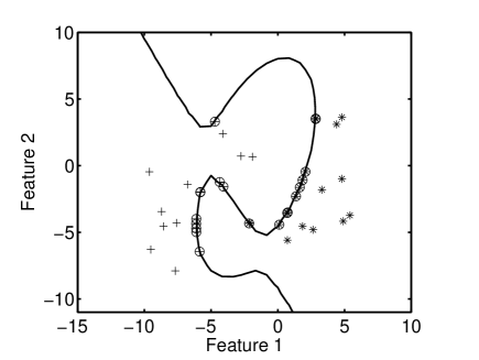
Rysunek 1: Example of the projection of a small set of objects on a nonlinear decision boundary.

The problem of defining consistent classification procedures is not the only one in domain learning. As it was already noticed, for a proper optimization, the distance from the objects to the decision boundary or to the domain boundary should be determined in the input space. Here, the original object representation is defined for the application, so the distances measured in this space are related in a meaningful way to the differences between objects. This relation does not hold for the output space of nonlinear decision functions. Still, well-performing classifiers may be obtained. The question, however, arises how evaluation and a comparison of classifiers that establish different nonlinearities,e.g. a linear classifier, a neural network and a support vector machine should be done.

The only way various classification functions can be compared is in their common input space, as their output spaces may differ. In the introduction, criterion (2) was adopted stating that the performance of a domain based classifier is determined by the classification of the most difficult example. It is determined by the distance in the input space from that object to the decision boundary. For linear classifiers the computation of this distance is straightforward. For analytical nonlinear classifiers the computation of this distance is not trivial, but might be defined based on some optimization procedure over the decision boundary. For arbitrary decision function, there is no way to derive this distance directly. In order to compare classifiers of various nature we propose the following heuristic procedure based on a stochastic approximation of the distance of an object to the decision boundary:

1. Let $f$ be a classifier found in the input space ${\mathbb{R}}^{m}$. Given an independent test set $S$, generate a large set of objects $R\in{\mathbb{R}}^{m}$ that lie in the neighborhood of the test examples.

2. Label the objects in $S$ and $R$ by the classifier $f$.

3. For each object $\mbox{$\mathbf{x}$}_{s}$ in $S$ find the $k$ nearest objects $\mbox{$\mathbf{x}$}^{i}_{r}$ in $R$ that are assigned different labels.

4. Enrich this set $\{\mbox{$\mathbf{x}$}^{i}_{r},i\!=\!1,2,\ldots,k\}$ by interpolation.

5. Use successive bisection to find the points $\mbox{$\mathbf{x}$}^{i}_{c}$ that are on the lines between $\mbox{$\mathbf{x}$}_{s}$ and all $\mbox{$\mathbf{x}$}^{i}_{r}$ such that they are almost on the decision boundary induced by $f$.

6. Find the point $\mbox{$\mathbf{x}$}_{c}$ in $\{\mbox{$\mathbf{x}$}^{i}_{c}\}$ that is nearest to $\mbox{$\mathbf{x}$}_{s}$.

7. Use the distance $d(\mbox{$\mathbf{x}$}_{s},\mbox{$\mathbf{x}$}_{c})$ between $\mbox{$\mathbf{x}$}_{s}$ and $\mbox{$\mathbf{x}$}_{c}$ as a measure for the confidence in the classification of $\mbox{$\mathbf{x}$}_{s}$. If the true label of $\mbox{$\mathbf{x}$}_{s}$ is known the distance to $\mbox{$\mathbf{x}$}_{c}$ may be given a sign: positive for a correct label, negative for an incorrect one.

8. Use

   $$e_{S}=min_{\mbox{$\mathbf{x}$}_{s}\in S}d(\mbox{$\mathbf{x}$}_{s},\mbox{$\mathbf{x}$}_{c})$$ (19)

   as a performance measure for the evaluated classifier $f$ given the test set $S$.

This proposed procedure has to be further evaluated. An example of the result of the projection of a small test set on a given classifier is shown in fig. 1.

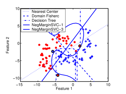
Rysunek 2: Five domain based classifiers on artificial data. The three support objects of the linear Negative Margin SVM are indicated by circles.

5 Example

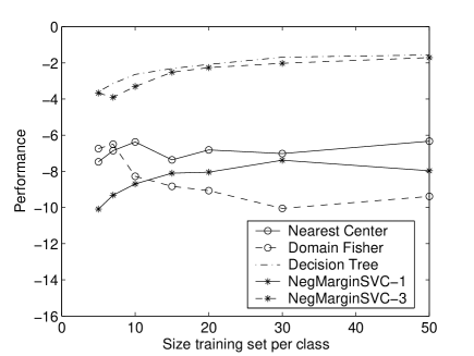
Rysunek 3: Learning curves for the five domain based classifiers. As classes overlap, the performance (19) is negative. Higher performance indicates better results.

We implemented the following domain based classifiers:

Nearest Center,

NCC, based on (5).

Domain Fisher

based on (11), using an heuristic estimate of $G$ by pre-whitening the data followed by the NCC to determine the class centers.

Decision Tree

using the purity criterion.

Negative Margin SVM

using a linear kernel. As the optimization problem is not quadratic, we implemented this classifier using boosting (Schapire02).

Negative Margin SVM

using a 3rd order polynomial kernel.

Two slightly overlapping artificial banana shaped classes are generated in two dimensions. Fig. 2 shows an example for $50$ objects per class. The decision boundaries for the above mentioned classifiers are also presented there.

The following experiment is performed using a fixed test set of $200$ examples per class. Training sets of the cardinalities up to $50$ objects per class are generated, such that smaller sets are contained in the larger ones. For each training set the above classifiers are determined and evaluated using the procedure discussed in section 4. This is repeated $10$ times and the performances is averaged.

Fig. 3 presents the results as a function of the cardinality of the training set. These are the learning curves of five classifiers showing an increasing performance as a function of the training size. As the classes slightly overlap, the performance (19) is negative. This is caused by the fact that the ’worst’ classified object in the test set is erroneously labeled and is, thereby on the wrong side of the decision boundary.

The curves indicate that our implementation of the Domain Fisher Discriminant is bad, at least for these data. This might be understood that it is sensitive for all class boundary points, to all sides. Enlarging the dataset may yield more disturbances. The simpler Nearest Center classifier performs much better and is about similar to the linear SVM. The nonlinear SVM as well as the Decision Tree yield very good results. Our evaluation procedure should bad for overlapping training sets classified by the Decision Tree, as small regions separated out in different classes disturb the procedure. They are, however, not detected if there size is really small. The probability that inside such a region a point is generated (compare the procedure discussed in section 4 may be too small.

6 Conclusions

Traditional ways of learning are inappropriate or inaccurate if training sets are only representative for the domain, but not for the distribution of the target objects. In this paper, a number of domain based classifiers have been discussed. Instead of minimizing the expected number of classification errors, the minimum distance to the decision boundary is proposed as a criterion. This is difficult to compute for arbitrary nonlinear classifiers. A heuristic procedure based on generating points close to the decision boundary is proposed for classifier evaluation.

This paper is restricted to an introduction to domain learning. It formulates the problem, points towards possible solutions and gives some examples. A first series of domain based classifiers has been implemented. Much research has to be done to make the domain based classification approach ready for applications. As there is a large need for novel approaches in this area, we believe that an important new theoretical direction for further investigation is identified.