TDOA Matrices: Algebraic Properties and their Application to Robust Denoising with Missing Data

Abstract

Measuring the Time delay of Arrival (TDOA) between a set of sensors is the basic setup for many applications, such as localization or signal beamforming. This paper presents the set of TDOA matrices, which are built from noise-free TDOA measurements, not requiring knowledge of the sensor array geometry. We prove that TDOA matrices are rank-two and have a special SVD decomposition that leads to a compact linear parametric representation. Properties of TDOA matrices are applied in this paper to perform denoising, by finding the TDOA matrix closest to the matrix composed with noisy measurements. The paper shows that this problem admits a closed-form solution for TDOA measurements contaminated with Gaussian noise which extends to the case of having missing data. The paper also proposes a novel robust denoising method resistant to outliers, missing data and inspired in recent advances in robust low-rank estimation. Experiments in synthetic and real datasets show significant improvements of the proposed denoising algorithms in TDOA-based localization, both in terms of TDOA accuracy estimation and localization error.

I Introduction

Time delay of arrival (TDOA) estimation is an essential pre-processing step for multiple applications in the context of sensor array processing, such as multi-channel source localization [1], self-calibration [2] and beamforming [3]. In all cases, performance is directly related to the accuracy of the estimated TDOAs [4].

Estimating TDOA in noisy environments has been subject of study during the last two decades [5, 6, 7], and is still an active area of research, benefiting from current advances in signal processing and optimization strategies [8, 9, 10, 11].

Typically, the TDOA between a single pair of sensors is obtained by measuring the peak of the generalized cross-correlation (GCC) of the received signals on each sensor [12], which are assumed to be generated from a single source. Many factors, such as the spectral content of the signal, multipath propagation, and noise contribute to errors in the estimation of the TDOA.

Given a set of sensors, TDOA measurements can be obtained for every possible pair of sensors. This is commonly known as the full TDOA set or spherical set [13]. This paper studies how to reduce noise and errors from the full TDOA set. The intuition behind this denoising is to exploit redundancy of the full TDOA set. For $n$ sensors, the full set of $n(n-1)/2$ measurements can be represented by $n-1$ values, which are referred to as the non-redundant set. This problem has been studied in the past, showing that one can optimally obtain the non-redundant set when TDOA measurements are contaminated with additive Gaussian noise. This is known as the Gauss-Markov estimator [14]. However, in more realistic scenarios errors are not Gaussian and some of the TDOA measurements may contain outliers. In these cases the Gauss-Markov estimator performs poorly.

This paper presents the TDOA matrix, which is created by the arrangement of the full TDOA set inside a skew-symmetric matrix, and studies the algebraic properties of this matrix, showing that it has rank $2$ and a SVD decomposition with $n-1$ degrees of freedom. Such matrices have been previously defined in the literature [15], but their properties and applications have not been studied until now.

These algebraic properties are used in this paper to perform denoising under different scenarios, which include the presence of missing TDOA measurements and outliers. These denoising algorithms are tested in the context of speaker localization with microphone arrays, using synthetic and publicly available real datasets. Our denoising algorithms are able to recover accurate TDOA values for high rates of missing data and outliers, significantly outperforming the Gauss-Markov estimator in those cases. All the proposed methods don’t require knowledge of the sensor positions, so that they can also be used for calibration [2].

The main contributions of this work are threefold: i) Definition of the algebraic properties of TDOA matrices. ii) A closed-form solution for TDOA denoising for Gaussian noise and the presence of missing data. iii) Novel robust-denoising methods for handling additive correlated noise, outliers and missing data.

I-A Notation

Real scalar values are represented by lowercase letters (e.g. $\delta$). Vectors are by default arranged column-wise and are represented by lowercase bold letters (e.g. $\mathbf{x}$). Matrices are represented by uppercase bold letters (e.g. $\mathbf{M}$). Lower-case letters are reserved to define vector and set sizes (e.g. vector $\mathbf{x}=(x_{1},\cdots,x_{n})^{\top}$ is of size $n$), and $\mathbf{x}^{\top}$ denotes transpose of vector $\mathbf{x}$. Calligraphic fonts are reserved to represent generic sets (e.g. $\mathcal{G}$) or functions applied to matrices (e.g. $\mathcal{P}(\mathbf{X})$). The $l_{2}$ norm $\|\cdot\|_{2}$ will be written by default as $\|\cdot\|$ for simplicity, and $\|\cdot\|_{F}$ is the Frobenius norm, while $|\cdot|$ is reserved to represent absolute values of scalars. The $l_{0}$ norm of a matrix, written $\|\cdot\|_{0}$, is defined as the number of non-zero elements of the matrix. $\mathbf{A}\,\circ\,\mathbf{B}$ is the Hadamard product between $\mathbf{A}$ and $\mathbf{B}$, defined as the entrywise multiplication of the corresponding matrices. $\operatorname{tr}(\cdot)$ is the trace function.

We also define the normalized unitary vector $\mathbf{\hat{1}}$ as $\mathbf{\hat{1}}=\nobreak\left(1,\dotsc,1\right)^{\top}/\sqrt{n}$, and the null vector $\mathbf{\hat{0}}$ as $\mathbf{\hat{0}}=\nobreak\left(0,\dotsc,0\right)^{\top}$, both of them having size $n$. Finally, $\mathds{1}=n~{}\mathbf{\hat{1}}\,\mathbf{\hat{1}}^{\top}$ is a $n\times n$ matrix with all elements equal to $1$, $\mathbf{D_{x}}$ is a $n\times n$ diagonal matrix where its main diagonal is the vector $\mathbf{x}$, and $\mathbf{I}$ is the identity matrix.

I-B Paper Structure

The rest of the paper is distributed as follows. Section II describes the related work and Section III the problem statement. In section IV TDOA matrices are described along with a derivation of their properties. TDOA denoising in Gaussian noise case is addressed in section V, also providing a closed-form solution. In sections VI and VII we propose novel algorithms for robust handling of noise and missing data, respectively. Section VIII combine the proposals of the previous two sections into an unified algorithm. We also provide an extensive experimentation to validate the proposed algorithms using both synthetic (Section IX) and real data (Section X). Finally, conclusions are drawn in section XI.

II Related Work

TDOA estimation is an essential first step for multiple applications related to 1) localization, 2) self-calibration and 3) beamforming (among others):

1) Localization: widely used in radar, sonar and acoustics, since no synchronization between the source and sensor is needed. The TDOA information is combined with knowledge of the sensors’ positions to generate a Maximum Likelihood spatial estimator made from hyperboloids intersected in some optimal sense. A linear closed-form solution of the former problem, valid when the TDOA estimation errors are small, is given in [16].

2) Self-calibration: since knowing the position of sensors is mandatory for localization techniques, some strategies have been also proposed in order to calibrate them using only TDOA measurements. In [17, 2], the TDOA problem is converted in a Time of Arrival (TOA) problem estimating the departure time of signals. Then, self-calibration techniques for TOA can be employed. The main drawback of this approach is that the conversion step from TDOA to TOA is very sensitive to outliers and correlated noise.

3) Beamforming: precise TDOA estimations is also critical for beamforming techniques and its applications. In [3], for example, additional steps are proposed for selecting the appropriate TDOA value among the correlation peaks, and also dealing with TDOA outliers. These steps include a Viterbi decoding based algorithm which maximizes the continuity of the TDOA estimations in several frames. However, the TDOA selection criteria is just based on their distance to surrounding TDOA values and their GCC-PHAT values, thus not attempting to benefit from the actual redundancy of the TDOA measurements.

Hence, an accurate estimation of TDOA is essential for a good performance of any of the former applications based on these measurements.

Typically, when only two sensors are employed, the peak of the generalized cross-correlation (GCC) function of the signals of two sensors is a good estimator for the TDOA, for reasonable noise and reverberation levels [12].

When more than two sensors are used ($n>2$), there are $n(n-1)/2$ different TDOA measurements from all possible pairs of sensors, forming the full TDOA set or spherical set [13]. However, all those TDOA measurements are redundant. In fact, usually one sensor is considered the reference sensor, and only the subset of $n-1$ TDOA measurements which involve that sensor are considered. That non-redundant set is the set of measurement used by the majority of TDOA-based positioning algorithms proposed in the literature [18, 16, 19, 20, 21, 22]. Nevertheless, an optimal (denoised) version of the non-redundant set can be estimated from the redundant set using a Bayesian Linear Unbiased Estimator (BLUE), also known as the Gauss-Markov estimator [14].

A closed-form solution for the BLUE estimator is provided in [23], also proving that it is equal to the standard least squares estimator, and that it reaches the Cramer-Rao lower bound for positioning estimation. However, all the results in that work are based on the assumption of additive Gaussian noise, which is unrealistic in many practical applications [24], and doesn’t yield good results when correlated noise is present as a consequence, for instance, of multipath propagation. Additionally, the experimental results shown in their work are only applied to synthetic data, thus not allowing to assess the performance of their proposal in real scenarios (in section X we show the limitations of their method when evaluated on real data).

A least-squares solution to TDOA denoising is proposed in [25]. It is based on projecting the non-redundant set of TDOA measurements into a set of “feasible” bivectors (rank 2, antisymmetric tensors) that show the same geometric properties of TDOA matrices. This denoising is also optimal for Gaussian noise but as in [24] the experimental analysis is based on simulated data and it does not cope with missing data or the presence of outliers in the TDOA measurements.

Periodicity in correlated signals, coherent noise and multi-path due to reverberation are the major sources of non-Gaussian error in TDOA estimation. Different approaches have been proposed to deal with them. A basic method consists in making the GCC function more robust, de-emphasizing the frequency-dependent weighting. The Phase Transform (PHAT) [26] is one example of this procedure which has received considerable attention as the basis of acoustic source localization systems due to its robustness in real world scenarios [27, 28]. Other approaches are based in blind estimation of multi-path (room impulse response) [29] but they need a good initialization to perform well.

Some previous works have also proposed more complicated structures in order to represent TDOA redundancy, while not imposing strong assumptions on the noise distribution. In [30] a representation based on graphs allows to disambiguate if a peak in correlation was generated by the direct path or by reverberation applying an efficient search algorithm among all possible combinations. However, they do not explicitly attempt to provide improved TDOA estimations by exploiting their redundancy.

Also different matrix representations have been used in the bibliography regarding TDOA formulation. For example [31] uses a representation slightly different to the TDOA matrices we describe here, but such representation does not have the algebraic properties that TDOA matrices have, and their authors do not address an study in this sense.

So, to the best of our knowledge, there are no previous reported work dealing with improving TDOA estimations by exploiting their redundancy, while not imposing Gaussian noise restrictions, not requiring the sensor positions, and being able to deal with the presence of outliers and missing measurements (errors that will severely impact the performance of applications based on TDOA measurements). In this paper we show that TDOA matrices are a powerful tool that combined with recent advances in robust low-rank estimation, are able to generate novel solutions for these problems.

III Problem Statement

Hereafter, we assume only one source located at the position $\mathbf{r}=(r_{x},r_{y},r_{z})^{\top}$, and $n$ sensors synchronized between them and placed in different positions ${\mathbf{s}_{i}=\nobreak(s_{ix},s_{iy},s_{iz})^{\top}},\,i\in\nobreak[1,n]$.

Given this setup, we will assume that the source is emitting an unknown signal $x(t)$. Then, the signal received by the sensor $i$, $x_{i}(t)$, is without loss of generality, a delayed and attenuated version of $x(t)$ (direct propagation) in addition to a signal $g_{i}(t)$ which summarizes all the adverse effects, i.e. noise, interference, multipath, etc. Thus, $x_{i}(t)=\nobreak x(t-\nobreak\tau_{i})+\nobreak g_{i}(t)$, where $\tau_{i}=\|\mathbf{r}-\mathbf{s}_{i}\|_{2}/c$ is the time of arrival (TOA) of the signal $x(t)$ at the sensor $\mathbf{s}_{i}$, being $c$ the propagation speed.

Assuming that TOA cannot be estimated directly, the time delay of arrival (TDOA) between the sensors $i$ and $j$ is estimated by correlating the received signals $x_{i}(t)$ and $x_{j}(t)$ (typically using the Generalized Cross-Correlation GCC [26]).

IV TDOA matrices

In this section we define TDOA matrices, and develop their main properties. In a nutshell, given any TDOA matrix $\mathbf{M}$, we show that: i) $\mathbf{M}$ is rank $2$ (Theorem 1), ii) $\mathbf{M}$ can be decomposed as $\mathbf{M}=\nobreak\left(\mathbf{x}\,\mathbf{\hat{1}}^{\top}-\mathbf{\hat{1}}\,\mathbf{x}^{\top}\right)$ with $\mathbf{x}=\mathbf{M}\,\mathbf{\hat{1}}$ (Lemma 1) and iii) the previous decomposition is bijective (Theorem 2).

These properties are the foundations of the denoising algorithms that we present in sections V and VI, and the missing data recovery proposal described in section VII, plus their combination described in section VIII.

IV-A Definition of TDOA matrices

Definition 1.

A TDOA matrix $\mathbf{M}$, is a $(n\times n)$ skew-symmetric matrix where the element $(i,j)$ is the time difference of arrival (TDOA) between the signals arriving at sensor $i$ and sensor $j$:

$$\mathbf{M}=\left\{\Delta\tau_{ij}\right\}=\begin{pmatrix}0&\Delta\tau_{12}&\cdots&\Delta\tau_{1n}\\ \Delta\tau_{21}&0&\cdots&\Delta\tau_{2n}\\ \vdots&\vdots&\ddots&\vdots\\ \Delta\tau_{n1}&\Delta\tau_{n2}&\cdots&0\end{pmatrix}$$ (1)

with

$$\Delta\tau_{ij}=\nobreak\left(\tau_{i}-\tau_{j}\right),$$ (2)

where $\tau_{i}$ is the time of arrival of the signal $x(t)$ at the sensor $\mathbf{s}_{i}$.

We will also express $\mathbf{M}$ in terms of its columns as $\mathbf{M}=\nobreak\left(\mathbf{m}_{1},\mathbf{m}_{2},\cdots,\mathbf{m}_{n}\right)$, being $\mathbf{m}_{i}=\nobreak\left(\Delta\tau_{1i},\Delta\tau_{2i},\ldots,\Delta\tau_{ni}\right)^{\top}$.

We denote as $\mathcal{M}_{T}(n)$ to the set of TDOA matrices of size $n\times n$.

Notice that there is a bijection between the full TDOA set and the corresponding TDOA matrix. Nevertheless expressing TDOA measurements as a matrix has important advantages, that we will discover throughout this article.

Note also that in the former definition, knowing the sensor array geometry is not required. For a given geometry, all the feasible TDOA matrices (those that are consistent with that particular geometry) are a subset of $\mathcal{M}_{T}(n)$. Studying the properties of such subset is out of the scope of this paper and the interested reader can refer to [8, 9, 32] for further details.

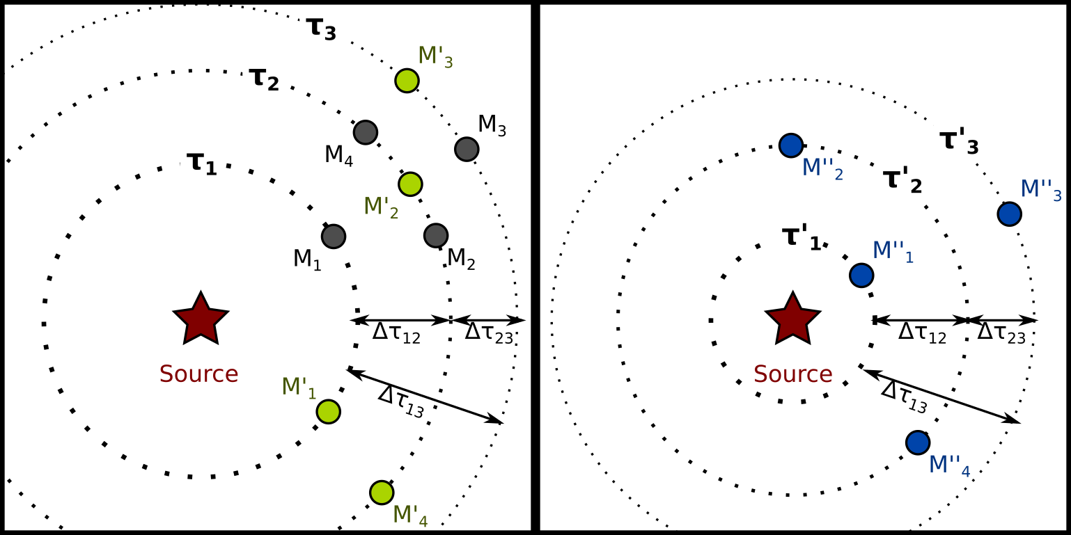
On the other hand, given a particular TDOA matrix, there are infinite number of sensors geometries which match with it. Left side of Fig. 1 shows that, given a set of TOAs ($\tau_{1}$,…, $\tau_{n}$) compatible with the set of TDOA measurements, the microphones can be situated in any place along the circumference (sphere in the 3D case) with center in the source (dotted lines), preserving its corespondent TOA (and therefore, its TDOA). Right side of Fig. 1 shows that there are a infinite number of TOA sets that comply with a given set of TDOA measurements.

Figure 1: Example of three different geometrical configurations (grey, green and blue) of 4 sensor with identical TDOA matrix.

IV-B Rank of TDOA matrices

Theorem 1.

Let $\mathbf{M}\in\mathcal{M}_{T}(n)$, then $\mathbf{M}$ is rank 2 or 0 (trivial case).

Proof:

The matrix $\mathbf{M}$ can be expressed as:

$$\mathbf{M}=\mathbf{T}-\mathbf{T}^{\top},$$ (3)

where $\mathbf{T}$ is a rank 1 matrix defined as:

$$\mathbf{T}=\begin{pmatrix}\tau_{1}&\cdots&\tau_{1}\\ \vdots&\ddots&\vdots\\ \tau_{n}&\cdots&\tau_{n}\end{pmatrix},$$ (4)

Applying the well known inequality:

$$\operatorname{rank}(\mathbf{A}+\mathbf{B})\leq\operatorname{rank}(\mathbf{A})+\operatorname{rank}(\mathbf{B}),$$ (5)

we can deduce that $\operatorname{rank}(\mathbf{M})\leq 2$.

Moreover, since the rank of any skew-symmetric matrix must be even, rank 1 is not feasible. So we can conclude that, excepting the case that $\mathbf{M}$ is the zero matrix (trivial case), the rank of $\mathbf{M}$ is 2. This completes the proof. ∎

Note that the formerly referred as ’trivial case’ only occurs when the time of arrival is the same for all the sensors, i.e sensors are geometrically placed on a sphere with center in the source.

Rank deficiency of TDOA matrices means that their rows and columns are linearly dependent. That is consistent with the fact that, in the noise-free case, the full TDOA set can be generated from the non-redundant set using linear equations [23]. In fact, in a TDOA matrix, the column $j$ is the TDOA non-redundant set when the sensor $j$ is the reference for TDOA measurements. Hereafter, and without loss of generality, we will consider the first sensor as the reference for the non redundant-set.

IV-C Bijective mapping for TDOA matrices

We show next a particular representation of TDOA matrices with $n-1$ parameters that describes their spectral properties and also forms the base for our denoising algorithms.

Theorem 2.

Let $H\subset\mathbb{R}^{n}$ be a $n-1$ dimensional hyperplane of $\mathbb{R}^{n}$ such that $\mathrm{span}(\hat{1})\nsubseteq H$, then there always exits an isomorphism between $\mathcal{M}_{T}(n)$ and $H$ of form:

$$\phi_{H}:H \longrightarrow\quad\mathcal{M}_{T}(n)$$

$$\mathbf{z} \longmapsto\mathbf{z}\,\mathbf{\hat{1}}^{\top}-\mathbf{\hat{1}}\,\mathbf{z}^{\top}$$

Proof:

Theorem 2 states that a bijective linear map exists between $\mathcal{M}_{T}(n)$ an a $n-1$ dimensional subset of $\mathbb{R}^{n}$. Since the matrix $\mathbf{T}$ in (4) can be rewritten as $\mathbf{T}=\mathbf{z}\,\mathbf{\hat{1}}^{\top}$, where $z=(\tau_{1},\cdots,\tau_{n})^{\top}$, we can define the following linear map:

$$\phi:\mathbb{R}^{n} \longrightarrow\quad\mathcal{M}_{T}(n)$$

$$\mathbf{z} \longmapsto\mathbf{z}\,\mathbf{\hat{1}}^{\top}-\mathbf{\hat{1}}\,\mathbf{z}^{\top}$$

that is clearly surjective but not injective. That is, any vector $\mathbf{z}^{\prime}=\mathbf{z}+\alpha\,\mathbf{\hat{1}}$ represents the same TDOA matrix. Indeed, the kernel of $\phi$ is the linear subspace of $\mathbb{R}^{n}$ generated by $\mathbf{\hat{1}}$.

Since we are looking for an isomorphism, we will restrict the domain of $\phi$ to ensure injectivity. It yields $\phi_{H}$, where $H\subset\mathbb{R}^{n}$ is a hyperplane of $\mathbb{R}^{n}$ not containing $\mathrm{ker}(\phi)$. Note that $\phi_{H}$ is bijective as $H\subset\mathbb{R}^{n}$ keeps the surjectivity of $\phi$ and, since $\mathrm{ker}(\phi_{H})=\{\mathbf{0}\}$, the function is also injective. ∎

Hereafter, we will only consider the particular case of $\phi_{H}$ for the hyperplane $H=\mathrm{ker}(\phi)^{\perp}$. It yields the following expression for any $M\in\mathcal{M}_{T}(n)$:

$$\mathbf{M}=\left(\mathbf{x}\,\mathbf{\hat{1}}^{\top}-\mathbf{\hat{1}}\,\mathbf{x}^{\top}\right)\quad,~{}~{}\,\mathbf{x}\perp\mathbf{\hat{1}}\quad,\mathbf{x}\in\mathbb{R}^{n}$$ (6)

Choosing $\mathbf{x}$ perpendicular to $\mathbf{\hat{1}}$ is very convenient, since both it simplifies $\phi_{H}^{-1}$ as shown in the corollary 2.1, and it also can be used for calculate the singular value decomposition (SVD) of any $M\in\mathcal{M}_{T}(n)$, as discussed in IV-C1. This leads to a parametric representation of $\mathbf{M}$ that has important properties that we will exploit later for TDOA denoising.

Corollary 2.1.

Given any $\mathbf{M}\in\mathcal{M}_{T}(n)$, the corresponding vector $\mathbf{x}\in\mathbb{R}^{n}$, perpendicular to $\mathbf{1}$, can be calculated as:

$$\mathbf{x}=\mathbf{M}\,\mathbf{\hat{1}}.$$ (7)

Corollary 2.2.

$\mathbf{M}\in\mathcal{M}_{T}(n)$ can also be expressed as:

$$\mathbf{M}=\frac{1}{\sqrt{n}}\left(\mathbf{D_{x}}\,\mathds{1}-\mathds{1}\,\mathbf{D_{x}}\right)\quad,\,\mathbf{\hat{1}}\perp\mathbf{\hat{x}},$$ (8)

since $\mathbf{x}\,\mathbf{\hat{1}}^{\top}=\mathbf{D_{x}}\,\mathds{1}/\sqrt{n}$ and $\mathbf{\hat{1}}\,\nobreak\mathbf{x}^{\top}=\nobreak\mathds{1}\,\nobreak\mathbf{D_{x}}/\sqrt{n}$,

IV-C1 Singular Value Decomposition

Because $\mathbf{M}\in\mathcal{M}_{T}(n)$ is a skew-symmetric matrix of rank 2, it has the following singular value decomposition (SVD) [33, Supplementary material]:

$$\mathbf{M}=\left(\mathbf{\hat{u}}_{2},-\mathbf{\hat{u}}_{1}\right)\begin{pmatrix}\sigma&0\\ 0&\sigma\end{pmatrix}\left(\mathbf{\hat{u}}_{1},\mathbf{\hat{u}}_{2}\right)^{\top}=\sigma\left(\mathbf{\hat{u}}_{2},-\mathbf{\hat{u}}_{1}\right)\left(\mathbf{\hat{u}}_{1},\mathbf{\hat{u}}_{2}\right)^{\top},$$ (9)

where $\mathbf{\hat{u}}_{1}$ and $\mathbf{\hat{u}}_{2}$ are orthonormal vectors and $\sigma\geq 0$. Note that the SVD decomposition of $\mathbf{M}$ is not unique. Given any orthogonal $2\times 2$ matrix $\mathbf{R}$, the vectors $\left(\mathbf{\hat{v}}_{1},\mathbf{\hat{v}}_{2}\right)=\left(\mathbf{\hat{u}}_{1},\mathbf{\hat{u}}_{2}\right)\,\mathbf{R}$ also represent a valid SVD decomposition:

$$\mathbf{M}=\sigma\left(\mathbf{\hat{v}}_{2},-\mathbf{\hat{v}}_{1}\right)\left(\mathbf{\hat{v}}_{1},\mathbf{\hat{v}}_{2}\right)^{\top}=\sigma\left(\mathbf{\hat{u}}_{2},-\mathbf{\hat{u}}_{1}\right)\left(\mathbf{\hat{u}}_{1},\mathbf{\hat{u}}_{2}\right)^{\top}.$$ (10)

Among all possible SVD decompositions of $\mathbf{M}$ note that theorem 2 guarantees that always exists one where $\mathbf{\hat{u}}_{1}=\mathbf{\hat{1}}$. In such case SVD decomposition can be computed from (6) as stated in the following theorem:

Lemma 1.

Given $\mathbf{M}\in\mathcal{M}_{T}(n)$, it admits the following SVD decomposition:

$$\mathbf{M}=\sigma\left(\mathbf{\hat{u}},-\mathbf{\hat{1}}\right)\left(\mathbf{\hat{1}},\mathbf{\hat{u}}\right)^{\top}\quad\text{with}\quad\mathbf{\hat{u}}=\dfrac{\mathbf{M}\,\mathbf{\hat{1}}}{\|\mathbf{M}\,\mathbf{\hat{1}}\|}\quad\sigma=\|\mathbf{M}\,\mathbf{\hat{1}}\|$$ (11)

Note that, according the previous lemma, not all rank 2 skew-symmetric matrices are TDOA-Matrices. In fact, if $\mathbf{\hat{v}}_{1}$ and $\mathbf{\hat{v}}_{2}$ in (10) are not coplanar with $\mathbf{\hat{1}}$ (i.e. $(\mathbf{\hat{1}}^{\top}\mathbf{\hat{v}}_{1})\mathbf{\hat{v}}_{1}+(\mathbf{\hat{1}}^{\top}\mathbf{\hat{v}}_{2})\mathbf{\hat{v}}_{2}\neq\mathbf{\hat{1}}$), then the resulting matrix is rank 2 and skew-symmetric but not a TDOA matrix.

V TDOA Denoising

In this section we propose a denoising strategy to deal with Gaussian noise in the estimated TDOA measurements, deriving a closed form solution for the proposed optimization problem. This solution is also compared with the Gauss-Markov Estimator.

V-A Denoising Strategy

We assume now that each TDOA measurement is contaminated with uncorrelated Gaussian noise $n_{ij}=-n_{ji}$, such that $\Delta\tilde{\tau}_{ij}=\Delta\tau_{ij}+n_{ij}$. Therefore, the measured TDOA matrix $\tilde{\mathbf{M}}=\left\{\Delta\tilde{\tau}_{ij}\right\}$ is also a skew-symmetric matrix, sum of a noise-free $\mathbf{M}\in\mathcal{M}_{T}(n)$ and a skew-symmetric matrix containing noise $\mathbf{N}=\left\{n_{ij}\right\}$:

$$\tilde{\mathbf{M}}=\mathbf{M}+\mathbf{N}.$$ (12)

Because of the noise, $\tilde{\mathbf{M}}\notin\mathcal{M}_{T}(n)$ and thus Theorem 1 is no longer satisfied. Consequently, the rank of $\tilde{\mathbf{M}}$ may be higher than two. Nevertheless, we will show that we can take advantage of the structure of TDOA matrices in order to denoise the measured data.

For denoising, we propose finding the closest $\mathbf{M}^{\ast}\in\nobreak\mathcal{M}_{T}(n)$, to the measured matrix $\tilde{\mathbf{M}}$, in the sense of the Frobenius norm. This approach yields the following optimization problem:

$$\mathbf{M}^{\ast}=\underset{\mathbf{M}\in\mathcal{M}_{T}(n)}{\operatorname{arg\,min}}\quad\left\|\tilde{\mathbf{M}}-\mathbf{M}\right\|_{F}^{2}.$$ (13)

V-B Closed-Form Solution

Theorem 3.

Problem (13) has the following closed form solution: $\mathbf{M}^{\ast}=(\tilde{\mathbf{M}}\,\mathds{1}+\mathds{1}\,\tilde{\mathbf{M}})/n$

Proof:

From (6), the denoising problem (13) is equivalent to the following constrained convex optimization problem:

$$\underset{\mathbf{x}}{\operatorname{minimize}} \left\|\tilde{\mathbf{M}}-\left(\mathbf{x}\,\mathbf{\hat{1}}^{\top}-\mathbf{\hat{1}}\,\mathbf{x}^{\top}\right)\right\|_{F}^{2}$$ (14)

$$\operatorname{subject\;to} \mathbf{\hat{1}}^{\top}\,\mathbf{x}=0.$$

Using the definition of Frobenius norm $\|\mathbf{A}\|_{F}^{2}=\operatorname{tr}(\mathbf{A}\mathbf{A}^{\top})$, and trace properties $\operatorname{tr}(\mathbf{A}\mathbf{B})=\operatorname{tr}(\mathbf{B}\mathbf{A})$ and $\operatorname{tr}(\mathbf{A})=\operatorname{tr}(\mathbf{A}^{\top})$ we rewrite the cost as:

$$\left\|\tilde{\mathbf{M}}-\left(\mathbf{x}\,\mathbf{\hat{1}}^{\top}-\mathbf{\hat{1}}\,\mathbf{x}^{\top}\right)\right\|_{F}^{2}=\\ =\operatorname{tr}\left(\left[\tilde{\mathbf{M}}-\left(\mathbf{x}\,\mathbf{\hat{1}}^{\top}-\mathbf{\hat{1}}\,\mathbf{x}^{\top}\right)\right]\left[\tilde{\mathbf{M}}-\left(\mathbf{x}\,\mathbf{\hat{1}}^{\top}-\mathbf{\hat{1}}\,\mathbf{x}^{\top}\right)\right]^{\top}\right)\\ =2\left(\mathbf{x}^{\top}\,\mathbf{x}-\mathbf{x}^{\top}\,\mathbf{\hat{1}}\,\mathbf{\hat{1}}^{\top}\,\mathbf{x}-\mathbf{\hat{1}}^{\top}\,\tilde{\mathbf{M}}^{\top}\,\mathbf{x}+\mathbf{\hat{1}}^{\top}\,\tilde{\mathbf{M}}\,\mathbf{x}\right)+\\ +\operatorname{tr}{\left(\tilde{\mathbf{M}}\,\tilde{\mathbf{M}}^{\top}\right)=f\left(\mathbf{x};\tilde{\mathbf{M}}\right)}.$$ (15)

To solve the constrained problem (14) we use the method of Lagrange multipliers, resulting in the following unconstrained equivalent:

$$\mathbf{x}^{\ast}\,=\,\underset{\mathbf{x},\lambda}{\operatorname{arg\,min}}\,\left[\Lambda\left(\mathbf{x};\lambda\right)\right],$$ (16)

where $\lambda$ is the Lagrange multiplier and

$$\Lambda\left(\mathbf{x};\lambda\right)=f\left(\mathbf{x};\tilde{\mathbf{M}}\right)+\lambda\mathbf{\hat{1}}^{\top}\,\mathbf{x}.$$ (17)

We find extrema in (17) by taking first derivatives with respect to both $\mathbf{x}$ and $\lambda$ and solving the following system:

$$\nabla\Lambda\left(\mathbf{x};\lambda\right)=\mathbf{\hat{0}}\,\Rightarrow\\ \begin{cases}4\mathbf{x}^{\top}\left(\mathbf{I}-\mathbf{\hat{1}}\,\mathbf{\hat{1}}^{\top}\right)+2\mathbf{\hat{1}}^{\top}\left(\tilde{\mathbf{M}}-\tilde{\mathbf{M}}^{\top}\right)+\lambda\mathbf{\hat{1}}^{\top}=\mathbf{\hat{0}}^{\top}\\ \mathbf{\hat{1}}^{\top}\,\mathbf{x}=0\\ \end{cases}$$

$$\mathbf{x}^{\ast} =\frac{\left(\tilde{\mathbf{M}}-\tilde{\mathbf{M}}^{\top}\right)\mathbf{\hat{1}}-\lambda\mathbf{\hat{1}}}{2}$$

$$\lambda^{\ast} =\frac{\mathbf{\hat{1}}^{\top}\left(\tilde{\mathbf{M}}-\tilde{\mathbf{M}}^{\top}\right)\mathbf{\hat{1}}}{2\mathbf{\hat{1}}^{\top}\,\mathbf{\hat{1}}}.$$ (18)

Given that the objective function is strictly convex, the solution to the system is unique, and therefore because the proposed solution ($\mathbf{x}^{\ast}$ and $\lambda^{\ast}$) satisfies the equations of a critical point, it is the global minimum

Since $\tilde{\mathbf{M}}$ is skew-symmetric $(\tilde{\mathbf{M}}-\tilde{\mathbf{M}}^{\top})=2\tilde{\mathbf{M}}$. Therefore, (18) becomes:

$$\mathbf{x}^{\ast} =\frac{2\tilde{\mathbf{M}}\,\mathbf{\hat{1}}-\lambda\mathbf{\hat{1}}}{2}=\tilde{\mathbf{M}}\,\mathbf{\hat{1}}$$ (19a)

$$\lambda =\frac{2\mathbf{\hat{1}}^{\top}\,\tilde{\mathbf{M}}\,\mathbf{\hat{1}}}{2\mathbf{\hat{1}}^{\top}\,\mathbf{\hat{1}}}=2\mathbf{\hat{1}}^{\top}\,\tilde{\mathbf{M}}\,\mathbf{\hat{1}}=0.$$ (19b)

In (19b) we use the fact that $\mathbf{\hat{1}}^{\top}\,\mathbf{A}\,\mathbf{\hat{1}}=0$ for $\mathbf{A}$ being a skew-symmetric matrix. Also, it is interesting to note from (19a) that $\mathbf{x}^{\ast}$ follows the same expression as the one stated in (6) for $\mathbf{x}$ in the noise-free case.

A compact expression for $\mathbf{M}^{\ast}$ can be easily derived from (19a) via (6):

$$\mathbf{M}^{\ast}=\left(\mathbf{\hat{1}},\tilde{\mathbf{M}}\,\mathbf{\hat{1}}\right)\left(-\tilde{\mathbf{M}}\,\mathbf{\hat{1}},\mathbf{\hat{1}}\right)^{\top}=\tilde{\mathbf{M}}\,\mathbf{\hat{1}}\,\mathbf{\hat{1}}^{\top}+\mathbf{\hat{1}}\,\mathbf{\hat{1}}^{\top}\,\tilde{\mathbf{M}}=\\ =(\tilde{\mathbf{M}}\,\mathds{1}+\mathds{1}\,\tilde{\mathbf{M}})/n.$$ (20)

This completes the proof. ∎

Since lemma 1 relates (6) with SVD, the proposed denoising approach can be considered as a version of Eckart-Young-Mirsky theorem [34, 35] constrained to TDOA matrices.

V-C Equivalence with the Gauss-Markov Estimator

By operating in (20), each element $(i,j)$ of the denoised matrix $\mathbf{M}^{\ast}$ is obtained as follows:

$$\mathbf{M}^{\ast}=\{\Delta\tau_{ij}^{\ast}\}=\left\{\frac{1}{n}\left(\sum_{k=1}^{n}{\Delta\tau_{ik}+\Delta\tau_{kj}}\right)\right\}.$$ (21)

The closed-form in (21) is identical to the one reported in [23, eq.(14)] as the Gauss-Markov estimator of the TDOA measurements, so that all the properties there can be extrapolated to this work. This is not surprising as the least-squares cost of (13) is optimal for Gaussian noise. The same denoising result was found in [25] by projecting TDOA measurements into the set of “feasible” bivectors in a least-squares sense. Under the assumption of Gaussian noise, we can conclude that [23, 25] and our denoising result in (21) are completely equivalent.

VI Robust TDOA Denoising

In some application scenarios, the assumption of uncorrelated white noise made in section V is fully unrealistic. In cases where the noise is correlated with the signal, measurements are prone to contain outliers in the TDOA measurements due to spurious peaks in the correlation. For such cases, a more complete model for the measured matrix is:

$$\tilde{\mathbf{M}}=\mathbf{M}+\mathbf{N}+\mathbf{S},$$ (22)

where $\mathbf{M}\in\mathcal{M}_{T}(n)$, $\mathbf{N}$ is a skew-symmetric matrix containing Gaussian noise, much like in (12), and the new matrix $\mathbf{S}$ models the addition of all the outliers. Since the number of outliers is usually small as compared with the number of measurements, we will assume $\mathbf{S}$ to be sparse and unknown.

In order to denoise $\tilde{\mathbf{M}}$, we propose solving the following optimization problem, finding both matrices $\mathbf{M}$ and $\mathbf{S}$:

$$\underset{\mathbf{M},\mathbf{S}}{\operatorname{minimize}} \left\|\tilde{\mathbf{M}}-\mathbf{M}-\mathbf{S}\right\|_{F}^{2}$$ (23)

$$\operatorname{subject\;to} \mathbf{M}\in\mathcal{M}_{T}(n)$$

$$\|\mathbf{S}\|_{0}<2k,$$

where $k$ is the maximum number of outliers supposed to be present in the TDOA measurements.

Robust denoising in (23) is a non-convex optimization problem with constraints that are not even differentiable. This kind of optimization problems have been explored in Robust PCA (RPCA) [36] or robust low-rank factorizations such in GoDec [37]. Despite TDOA matrices are low-rank, these algorithms are not well suited here as they do not include all the algebraic constraints in TDOA matrices.

In order to solve (23), we propose an iterative algorithm, inspired in GoDec. It consists of an alternation method in which $\mathbf{M}$ and $\mathbf{S}$ are obtained in turns, with close-form solutions for these two steps (we use a subindex $t$ to denote the iteration count):

$$\left\{\begin{aligned} \mathbf{M}_{t}&=\underset{\mathbf{M}\in\mathcal{M}_{T}(n)}{\operatorname{arg\,min}}\quad\left\|\tilde{\mathbf{M}}-\mathbf{M}-\mathbf{S}_{t-1}\right\|_{F}^{2}\\ \mathbf{S}_{t}&=\underset{\|\mathbf{S}\|_{0}<2k}{\operatorname{arg\,min}}\quad\left\|\tilde{\mathbf{M}}-\mathbf{M}_{t}-\mathbf{S}\right\|_{F}^{2}\\ \end{aligned}\right.$$ (24)

The first sub-problem of (24) is the same as our denoising problem in (13), therefore $\mathbf{M}_{t}$ can be updated via (20). Then, $\mathbf{S}_{t}$ is updated via entry-wise hard thresholding of $\tilde{\mathbf{M}}-\mathbf{M}_{t}$. Thus:

$$\left\{\begin{aligned} \mathbf{M}_{t}&=\left(\tilde{\mathbf{M}}-\mathbf{S}_{t-1}\right)\,\mathbf{\hat{1}}\mathbf{\hat{1}}^{\top}+\mathbf{\hat{1}}\mathbf{\hat{1}}^{\top}\left(\tilde{\mathbf{M}}-\mathbf{S}_{t-1}\right)\\ \mathbf{S}_{t}&=\mathcal{P}_{2k}\left(\tilde{\mathbf{M}}-\mathbf{M}_{t}\right)\end{aligned}\right.$$ (25)

where $\mathcal{P}_{l}(\mathbf{X})$ is an function which generates a matrix with the same size of $\mathbf{X}$, preserving the $l$ elements of $\mathbf{X}$ with the largest absolute value, and making the rest of elements zero. Note that, since $\mathbf{X}$ is skew symmetric in our application, the result provided by $\mathcal{P}_{2k}(\cdot)$ is also skew symmetric. The convergence to a local minimum of this algorithm is guaranteed in similar circumstances as GoDec [37], as the solutions to both sub-problems in (25) are solved globally.

So, the proposed robust denoising algorithm is shown in Alg. 1.

Algorithm 1 Robust denoising.

Require: $\tilde{\mathbf{M}}$, $k$, $\epsilon$

Ensure: $\mathbf{M}\in\mathcal{M}_{T}(n)$, $\|\mathbf{S}\|_{0}<2k$,

  1:  $\mathbf{M}_{0}=\tilde{\mathbf{M}}$ ; $\mathbf{S}_{0}=0$ ; $t=0$

  2:  while $\|\tilde{\mathbf{M}}-\mathbf{M}_{t}-\mathbf{S}_{t}\|_{F}^{2}/\|\tilde{\mathbf{M}}\|_{F}^{2}>\epsilon$ do

  3:      $t=t+1$

  4:      $\mathbf{M}_{t}=(\tilde{\mathbf{M}}-\mathbf{S}_{t-1})\mathbf{\hat{1}}\mathbf{\hat{1}}^{\top}+\mathbf{\hat{1}}\mathbf{\hat{1}}^{\top}(\tilde{\mathbf{M}}-\mathbf{S}_{t-1})$

  5:      $\mathbf{S}_{t}=\mathcal{P}_{2k}(\tilde{\mathbf{M}}-\mathbf{M}_{t})$

  6:  end while

  7:  return $\mathbf{M}_{t}$, $\mathbf{S}_{t}$

From now on, we will refer to this algorithm as Robust DeN.

VII Missing Data Recovery

VII-A Recovery Strategy

In real scenarios, there may be situations where some of the elements of $\mathbf{\tilde{M}}$ might not be available (for instance, due to communications failure) or even when they are available, there are reasons to avoid using them (for example, due to a priori knowledge of unreliable measurements, or when calculating the whole redundant set is computationally too demanding) [32]. In such cases, we want to be able to avoid some measurements, thus performing estimations when part of the values in $\mathbf{\tilde{M}}$ are missing.

In this section, we address the matrix completion problem ([38, 39]) for TDOA matrices. We assume that in a measured TDOA matrix $\mathbf{\tilde{M}}$, some of its elements are unknown, and the rest are contaminated with additive Gaussian noise. We take advantage of the redundancy present in TDOA matrices to estimate a complete denoised TDOA matrix including the missing entries.

The matrix completion problem is stated as follows:

$$\mathbf{M}^{\ast}=\underset{\mathbf{M}\in\mathcal{M}_{T}(n)}{\operatorname{arg\,min}}\quad\left\|\mathbf{L}\,\circ\,\left(\tilde{\mathbf{M}}-\mathbf{M}\right)\right\|_{F}^{2},$$ (26)

where $\mathbf{L}$ is a symmetric binary matrix whose element $(i,j)$ is $1$ if the TDOA between the sensor $i$ and $j$ is known, being $0$ otherwise. For convenience and without loss of generality, the elements on the main diagonal of $\mathbf{L}$ will be set to $1$.

Solving (26) is equivalent to finding the full TDOA matrix whose elements best fit the available elements of $\mathbf{\tilde{M}}$. Note that, $\mathbf{L}\,\circ\,(\tilde{\mathbf{M}}-\mathbf{M})=(\tilde{\mathbf{M}}_{\mathbf{L}}-\mathbf{L}\,\circ\,\mathbf{M})$, where $\tilde{\mathbf{M}}_{\mathbf{L}}=(\mathbf{L}\,\circ\,\tilde{\mathbf{M}})$ is the result of setting the unknown elements of $\mathbf{\tilde{M}}$ to zero.

VII-B Closed-Form Solution

Theorem 4.

The problem (26) has the following closed form solution: $\mathbf{M}^{\ast}=\left(\mathbf{D_{\beta}}+\mathbf{\bar{L}}\right)^{-1}\tilde{\mathbf{M}}_{\mathbf{L}}\,\mathds{1}+\mathds{1}\tilde{\mathbf{M}}_{\mathbf{L}}\left(\mathbf{D_{\beta}}+\mathbf{\bar{L}}\right)^{-1}$ where $\mathbf{D_{\beta}}=\left(\mathbf{I}\,\circ\,\mathbf{L}\mathbf{L}^{\top}\right)$ is a $n\times n$ diagonal matrix with $\boldsymbol{\beta}=\left(n-\bar{\beta}_{1},\cdots,n-\bar{\beta}_{n}\right)^{\top}=\sqrt{n}\,\mathbf{L}\,\mathbf{\hat{1}}$ as its main diagonal. $\bar{\beta}_{i}$ is the number of missing measurements with the sensor $i$.

Proof:

Using Corollary 2.2, problem (26) is rewritten as

$$\underset{\mathbf{x}}{\operatorname{minimize}} \left\|\tilde{\mathbf{M}}_{\mathbf{L}}-\frac{\mathbf{L}\,\circ\,\left(\mathbf{D_{x}}\mathds{1}-\mathds{1}\mathbf{D_{x}}\right)}{\sqrt{n}}\right\|_{F}^{2}$$ (27)

$$\operatorname{subject\;to} \mathbf{\hat{1}}^{\top}\,\mathbf{x}=0.$$

Since $\mathds{1}$ is the identity element of the hadamard product and $\mathbf{D_{x}}$ is a diagonal matrix, we can rewrite (27) as:

$$\underset{\mathbf{x}}{\operatorname{minimize}} \left\|\tilde{\mathbf{M}}_{\mathbf{L}}-\frac{\left(\mathbf{D_{x}}\mathbf{L}-\mathbf{L}\mathbf{D_{x}}\right)}{\sqrt{n}}\right\|_{F}^{2}$$ (28)

$$\operatorname{subject\;to} \mathbf{\hat{1}}^{\top}\,\mathbf{x}=0.$$

Operating in a similar manner to (15) we get:

$$\left\|\tilde{\mathbf{M}}_{\mathbf{L}}-\frac{\left(\mathbf{D_{x}}\mathbf{L}-\mathbf{L}\mathbf{D_{x}}\right)}{\sqrt{n}}\right\|_{F}^{2}=\frac{2}{n}\operatorname{tr}\left(\mathbf{D_{x}}\mathbf{L}\mathbf{L}^{\top}\mathbf{D_{x}}\right)-\\ -\frac{2}{n}\operatorname{tr}\left(\mathbf{D_{x}}\mathbf{L}\mathbf{D_{x}}\mathbf{L}\right)+\frac{2}{\sqrt{n}}\operatorname{tr}\left(\left[\tilde{\mathbf{M}}_{\mathbf{L}}-\tilde{\mathbf{M}}_{\mathbf{L}}^{\top}\right]\mathbf{D_{x}}\mathbf{L}\right)+\\ +\operatorname{tr}\left(\tilde{\mathbf{M}}_{\mathbf{L}}\tilde{\mathbf{M}}_{\mathbf{L}}^{\top}\right).$$ (29)

Using the identity $\mathbf{x}^{\ast}\left(\mathbf{A}\,\circ\,\mathbf{B}\right)\mathbf{y}=\operatorname{tr}\left(\mathbf{D_{x}}^{\ast}\mathbf{A}\mathbf{D_{y}}\mathbf{B}^{\top}\right)$ we get:

$$\left\|\tilde{\mathbf{M}}_{\mathbf{L}}-\frac{\left(\mathbf{D_{x}}\mathbf{L}-\mathbf{L}\mathbf{D_{x}}\right)}{\sqrt{n}}\right\|_{F}^{2}=\frac{2}{n}\mathbf{x}^{\top}\,\left(\mathbf{I}\,\circ\,\mathbf{L}\mathbf{L}^{\top}\right)\,\mathbf{x}\\ -\frac{2}{n}\mathbf{x}^{\top}\,\left(\mathbf{L}\,\circ\,\mathbf{L}^{\top}\right)\,\mathbf{x}+2\,\mathbf{\hat{1}}^{\top}\,\left(\left[\tilde{\mathbf{M}}_{\mathbf{L}}-\tilde{\mathbf{M}}_{\mathbf{L}}^{\top}\right]\,\circ\,\mathbf{L}^{\top}\right)\,\mathbf{x}+\\ +\operatorname{tr}\left(\tilde{\mathbf{M}}_{\mathbf{L}}\tilde{\mathbf{M}}_{\mathbf{L}}^{\top}\right)=g\left(\mathbf{x};\tilde{\mathbf{M}},\,\mathbf{L}\right)$$ (30)

and finally:

$$\left\|\tilde{\mathbf{M}}_{\mathbf{L}}-\frac{\left(\mathbf{D_{x}}\mathbf{L}-\mathbf{L}\mathbf{D_{x}}\right)}{\sqrt{n}}\right\|_{F}^{2}=\\ \frac{2}{n}\left(\mathbf{x}^{\top}\,\mathbf{D_{\beta}}\,\mathbf{x}-\mathbf{x}^{\top}\,\mathbf{L}\,\mathbf{x}+n\,\mathbf{\hat{1}}^{\top}\,\left(\tilde{\mathbf{M}}_{\mathbf{L}}-\tilde{\mathbf{M}}_{\mathbf{L}}^{\top}\right)\,\mathbf{x}\right)+\\ +\operatorname{tr}\left(\tilde{\mathbf{M}}_{\mathbf{L}}\tilde{\mathbf{M}}_{\mathbf{L}}^{\top}\right)=g(\mathbf{x};\tilde{\mathbf{M}},\,\mathbf{L}).$$ (31)

It is important to note that equations (15) and (31) are identical when there is no missing data in $\tilde{\mathbf{M}}$ (i.e $\mathbf{L}=\mathds{1}=n\,\mathbf{\hat{1}}\,\mathbf{\hat{1}}^{\top}$ and $\mathbf{D_{\beta}}=n\,\mathbf{I}$).

We use the method of Lagrange multipliers to express (27) as the following unconstrained optimization problem:

$$\Lambda\left(\mathbf{x};\lambda\right)=g\left(\mathbf{x};\tilde{\mathbf{M}},\,\mathbf{L}\right)+\lambda\mathbf{\hat{1}}^{\top}\,\mathbf{x}.$$ (32)

By taking derivatives we obtain the following system:

$$\nabla\Lambda\left(\mathbf{x};\lambda\right)=\mathbf{\hat{0}}\,\Rightarrow\\ \begin{cases}\frac{2}{n}\mathbf{x}^{\top}\left(\mathbf{D_{\beta}}-\mathbf{L}\right)+\mathbf{\hat{1}}^{\top}\left(\tilde{\mathbf{M}}_{\mathbf{L}}-\tilde{\mathbf{M}}_{\mathbf{L}}^{\top}\right)+\lambda\mathbf{\hat{1}}^{\top}=\mathbf{\hat{0}}\\ \mathbf{\hat{1}}^{\top}\mathbf{x}=0.\end{cases}$$ (33)

Since $\mathbf{\hat{1}}^{\top}\mathbf{x}=0$ implies that $\mathds{1}\mathbf{x}=\mathbf{\hat{0}}$, we substitute in (33) obtaining:

$$\frac{2}{n}\left(\mathbf{D_{\beta}}+\mathbf{\bar{L}}\right)\mathbf{x}=\left(\tilde{\mathbf{M}}_{\mathbf{L}}-\tilde{\mathbf{M}}_{\mathbf{L}}^{\top}\right)\mathbf{\hat{1}}-\lambda\mathbf{\hat{1}},$$ (34)

where $\left(\mathbf{\bar{L}}=\mathds{1}-\mathbf{L}\right)$ (logical not operator over all elements of $\mathbf{L}$). Note that: $(\mathbf{D_{\beta}}+\mathbf{\bar{L}})$ is symmetric and, furthermore, $\mathbf{\hat{1}}$ is one of its eigenvectors.

$$\left(\mathbf{D_{\beta}}+\mathbf{\bar{L}}\right)\mathbf{\hat{1}}=\frac{\boldsymbol{\beta}+\boldsymbol{\bar{\beta}}}{\sqrt{n}}=n\mathbf{\hat{1}}.$$ (35)

Therefore, if the two terms of (34) are multiplied on the right by $\mathbf{\hat{1}}^{\top}$ we get:

$$2\,\mathbf{\hat{1}}^{\top}\mathbf{x}=\mathbf{\hat{1}}^{\top}\left(\tilde{\mathbf{M}}_{\mathbf{L}}-\tilde{\mathbf{M}}_{\mathbf{L}}^{\top}\right)\mathbf{\hat{1}}-\lambda.$$ (36)

Then applying to (36) the fact that

$$\mathbf{\hat{1}}^{\top}\mathbf{x}=0\quad\text{and}\quad\mathbf{\hat{1}}^{\top}(\tilde{\mathbf{M}}_{\mathbf{L}}-\tilde{\mathbf{M}}_{\mathbf{L}}^{\top})\mathbf{\hat{1}}=0,$$ (37)

we can conclude that $\lambda=0$. Thus, the solution of (27) is:

$$\mathbf{x}^{\ast}=n\left(\mathbf{D_{\beta}}+\mathbf{\bar{L}}\right)^{-1}\tilde{\mathbf{M}}_{\mathbf{L}}\mathbf{\hat{1}}.$$ (38)

Finally, the solution of problem (26) can be calculated from (38) using (6):

$$\mathbf{M}^{\ast}=\left(\mathbf{D_{\beta}}+\mathbf{\bar{L}}\right)^{-1}\tilde{\mathbf{M}}_{\mathbf{L}}\,\mathds{1}+\mathds{1}\tilde{\mathbf{M}}_{\mathbf{L}}\left(\mathbf{D_{\beta}}+\mathbf{\bar{L}}\right)^{-1}$$ (39)

This completes the proof. ∎

From now on, we will refer to this algorithm as MC. It is noteworthy to comment that the matrix $(\mathbf{D_{\beta}}+\mathbf{\bar{L}})$ contains important information about the recoverability of missing data: if it is full-rank, then the solution of (26) is unique and if $(\mathbf{D_{\beta}}+\mathbf{\bar{L}})$ is rank-deficient, missing data is not recoverable uniquely without any further assumption.

Furthermore, in the absence of missing data, $n(\mathbf{D_{\beta}}+\nobreak\mathbf{\bar{L}})^{-1}=\nobreak\mathbf{I}$, hence the matrix completion solution in (39) becomes the solution of the denoising problem stated in (20).

VIII Robust TDOA Denoising with Missing Data

In this section we aim to combine the results of sections VI and VII, addressing the more general case in which both outliers and missing data are considered. Therefore, the problem is a combination of (23) and (26) defined as:

$$\underset{\mathbf{M},\mathbf{S}}{\operatorname{minimize}} \left\|\mathbf{L}\,\circ\,\left(\tilde{\mathbf{M}}-\mathbf{M}-\mathbf{S}\right)\right\|_{F}^{2}$$ (40)

$$\operatorname{subject\;to} \mathbf{M}\in\mathcal{M}_{T}(n)$$

$$\|\mathbf{S}\|_{0}<2k$$

$$\mathbf{S}=\mathbf{L}\,\circ\,\mathbf{S}.$$

In the same way as in section VI, (40) can be solved by alternatively solving the following two subproblems until convergence:

$$\mathbf{M}_{t} =\underset{\mathbf{M}\in\mathcal{M}_{T}(n)}{\operatorname{arg\,min}}\quad\left\|\mathbf{L}\,\circ\,\left(\tilde{\mathbf{M}}-\mathbf{M}-\mathbf{S}_{t-1}\right)\right\|_{F}^{2}$$ (41a)

$$\mathbf{S}_{t} =\underset{\|\mathbf{S}\|_{0}<2k}{\operatorname{arg\,min}}\quad\left\|\mathbf{L}\,\circ\,\left(\tilde{\mathbf{M}}-\mathbf{M}_{t}\right)-\mathbf{S}\right\|_{F}^{2}.$$ (41b)

The subproblem (41a) is equivalent to the missing data problem solved in section VII but considering $\tilde{\mathbf{M}}_{\mathbf{L}}=\nobreak({\mathbf{L}\,\circ\,\tilde{\mathbf{M}}}-\nobreak\mathbf{S}_{t-1})$. Therefore, according to theorem 4, it has a closed form solution:

$$\mathbf{M}_{t}^{\ast}=(\mathbf{D_{\beta}}+\mathbf{\bar{L}})^{-1}(\mathbf{L}\,\circ\,\tilde{\mathbf{M}}-\mathbf{S}_{t-1})\,\mathds{1}+\\ +\mathds{1}(\mathbf{L}\,\circ\,\tilde{\mathbf{M}}-\mathbf{S}_{t-1})(\mathbf{D_{\beta}}+\mathbf{\bar{L}})^{-1}.$$ (42)

Since (41b) is of the same form as the second subproblem in (24), it can also be solved by entry-wise hard thresholding of $\mathbf{L}\,\circ\,(\tilde{\mathbf{M}}-\mathbf{M}_{t})$.

The pseudocode shown in Alg. 2 summarizes the proposed algorithm for the general case.

Algorithm 2 Robust denoising with missing data.

Require: $\tilde{\mathbf{M}}$, $\mathbf{L}$, $k$, $\epsilon$

Ensure: $\mathbf{M}\in\mathcal{M}_{T}(n)$, $\|\mathbf{S}\|_{0}<2k$,

  1:  $\mathbf{D_{\beta}}=\mathbf{I}\,\circ\,\mathbf{L}\mathbf{L}^{\top}$

  2:  $\mathbf{Q}=(\mathbf{D_{\beta}}+\mathbf{\bar{L}})^{-1}$

  3:  $\mathbf{M}_{0}=\tilde{\mathbf{M}}$ ; $\mathbf{S}_{0}=0$ ; $t=0$

  4:  while $\|\tilde{\mathbf{M}}-\mathbf{M}_{t}-\mathbf{S}_{t}\|_{F}^{2}/\|\tilde{\mathbf{M}}\|_{F}^{2}<\epsilon$ do

  5:      $t=t+1$

  6:      $\mathbf{M}_{t}=\mathbf{Q}(\mathbf{L}\,\circ\,\tilde{\mathbf{M}}-\mathbf{S}_{t-1})\,\mathds{1}+\mathds{1}(\mathbf{L}\,\circ\,\tilde{\mathbf{M}}-\mathbf{S}_{t-1})\mathbf{Q}$

  7:      $\mathbf{S}_{t}=\mathcal{P}_{2k}(\tilde{\mathbf{M}}-\mathbf{M}_{t})$

  8:  end while

  9:  return $\mathbf{M}_{t}$, $\mathbf{S}_{t}$

Note that in line 2 the matrix $\mathbf{Q}=(\mathbf{D_{\beta}}+\mathbf{\bar{L}})^{-1}$ can be precalculated in order to get an efficient implementation of the algorithm.

From now on, we will refer to this algorithm as Robust DeN+MC.

IX Experiments with Synthetic Data

In this section computer simulations will be used to compare the proposed algorithms with some of the alternatives existing in the state of the art.

For evaluating the Robust DeN and Robust DeN+MC algorithms, two different metrics will be used:

• The Signal-to-Noise-Ratio SNR [dB] of the non-redundant set referenced to the first sensor ($10\log(\sum_{i=1}^{n}{\|\Delta\tau_{i1}\|^{2}/\sum_{i=1}^{n}{\|\Delta{\tau}_{i1}^{\ast}-\Delta\tau_{i1}\|^{2}}})$). This is an application independent metric (where $\Delta{\tau}_{i1}^{\ast}$ is the estimation of $\Delta\tau_{i1}$), that will allow assessing the proposal improvements in the TDOA measurements per se.

• The localization error, measured as the average distance between the source ground truth position and the position estimated using any given localization algorithm based on TDOA estimations (such as [16] in our case). This is an application dependent metric, that will allow assessing the actual benefits of the proposal in an example of a real task. Note that our proposal is not restricted to localization and can be used in other applications that could benefit from denoised TDOAs (such as self-calibration or beamforming).

IX-A Experimental setup

For all the synthetic data experiments, a set of 10 sensors (which implies 45 different sensor pairs) and 1 source were randomly located. Therefore, 45 different TDOA measurements were generated per experiment, and independent Gaussian noise was added to them, using the same variance for all the measurements.

The sensor locations were uniformly distributed in a cube of 1 meter side, and the source positions were uniformly distributed in a 2 meter side cube. The propagation speed of the signal was set to 343.313 m/s. In all the experiments where it’s required, $\epsilon$ is set to $10^{-10}$. To increase the statistical significance of the results, they are provided as averages of 20 independent runs.

IX-B Evaluation of Robust TDOA Denoising

In this first experiment, we evaluated the performance of the Robust DeN algorithm proposed in section VI, imposing that some TDOA values were outliers. To simulate this, we randomly chose some measurements (between 0 and 10) and replaced them with a zero-mean Gaussian distributed noise, with a standard deviation of 0.1 ms. It is worth mentioning that the outlier values calculated that way are not related at all to the real TDOAs, thus being true outliers. The parameter $k$ of the proposed algorithm, which fixes the maximum number of identifiable outliers, was set to 8.

IX-B1 SNR Improvements Evaluation

Fig. 2a shows the SNR values for the Robust DeN algorithm when modifying the noise standard deviation and the number of outliers, compared with that obtained by the Gauss-Markov estimator (Fig. 2b), and also when only the non redundant set is used, i.e. not using the redundancy of TDOA measurements (Fig. 2c).

Figure 2: Robust denoising in synthetic data: SNR in dB, higher is better.

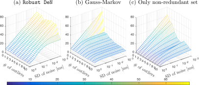
As predicted in section V, when no outliers are present, the performance of the Robust DeN algorithm is the same as Gauss-Markov (see row 0 in Figs. 2a and 2b), hence it reaches the Cramer-Rao Bound [23], while being much better than using no redundancy. Nevertheless, the proposed algorithm clearly outperforms the other two approaches when outliers are present in the measurements (rows 1 through 10 in the graphics of Fig. 2).

IX-B2 Source Localization Improvements Evaluation

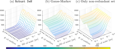
The optimized non redundant set provided by the algorithms applied in Section IX-B1 were used in a localization algorithm using [16]. The average localization errors (in mm) are shown in Fig. 3. Again, the Robust DeN algorithm performs as Gauss-Markov when there are no outliers, but is clearly superior when outliers are present.

It is also worth mentioning that the behaviour of the robust denoising keeps the improvements at roughly the same level for increasing number of outliers present, thus validating the ability of the algorithm to pinpoint and eliminate their presence.

Figure 3: Robust denoising in synthetic data: Localization error in mm (using [16]), lower is better.

IX-C Evaluation of Missing Data Recovery

In this second experiment, we evaluated the capability of the MC algorithm proposed in section VII to recover missing values. For our purposes, the missing TDOA measurements were also chosen randomly but, in contrast to the previous experiment, the matrix positions of the missing measurements were known.

Fig. 4 and Fig. 5 show, respectively, the SNR values, and the localization error for the MC algorithm, when modifying the noise standard deviation and the percentage of missing TDOA values in the TDOA matrix, as compared with using only the non-redundant set (missing values were set to zero).

Figure 4: Missing data recovery in synthetic data: SNR in dB, higher is better.

Figure 5: Missing data recovery in synthetic data: Localization error in mm (using [16]), lower is better.

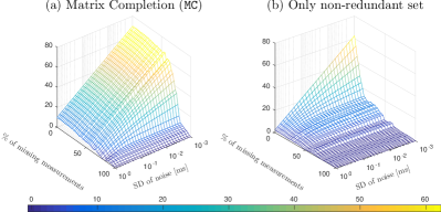
From the figures, it can be clearly seen that the proposed algorithm can take advantage of the knowledge about which measurements were missing, achieving even better results than when the positions of the outliers were unknown. For example, removing 50% of the full TDOA set of measurements implies 23 missing values of 45 measurements , much more than the maximum of 10 outliers evaluated in Fig. 2, while keeping good performance.

IX-D Evaluation of Robust TDOA Denoising with Missing Data

In this third experiment, we evaluated the capability of the Robust DeN+MC algorithm proposed in section VIII to face both outliers and recover missing values.

To provide a wide range of evaluation scenarios, we defined: i) Two conditions related to noise, namely low and high. The former corresponds to a standard deviation of $10^{-3}$ ms., and the latter to $0.2$ ms. ii) Two conditions related to the presence of outliers, imposing the existence of 2 or 6 outliers. iii) A variable number of missing TDOA measurements, defined as a percentage of missing TDOA values in the TDOA matrix.

In all cases, the number of outliers is fixed among the full TDOA set and then, some measurements are discarded, i.e. some of the discarded measurements may be outliers. Note that this is consistent with the real case, where it is not possible to anticipate where the outliers are.

Fig. 6 and Fig. 7 show, respectively, the SNR values, and the localization error for different algorithms, and for different evaluation scenarios.

(a) SNR with low noise and 2 outliers

(b) SNR with low noise and 6 outliers

(c) SNR with high noise and 2 outliers

(d) SNR with high noise and 6 outliers

Figure 6: Algorithm evaluation in synthetic data: SNR in dB.

(a) Localization error with low noise and 2 outliers

(b) Localization error with low noise and 6 outliers

(c) Localization error with high noise and 2 outliers

(d) Localization error with high noise and 6 outliers

Figure 7: Algorithm evaluation in synthetic data: Localization error in mm ([16] is used for source position estimation from the optimized TDOA values).

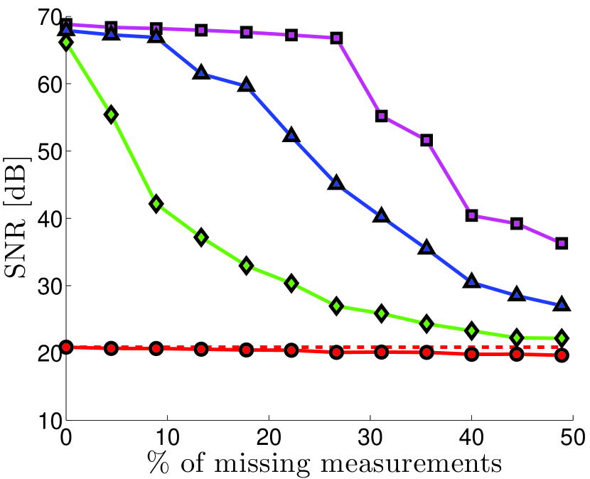
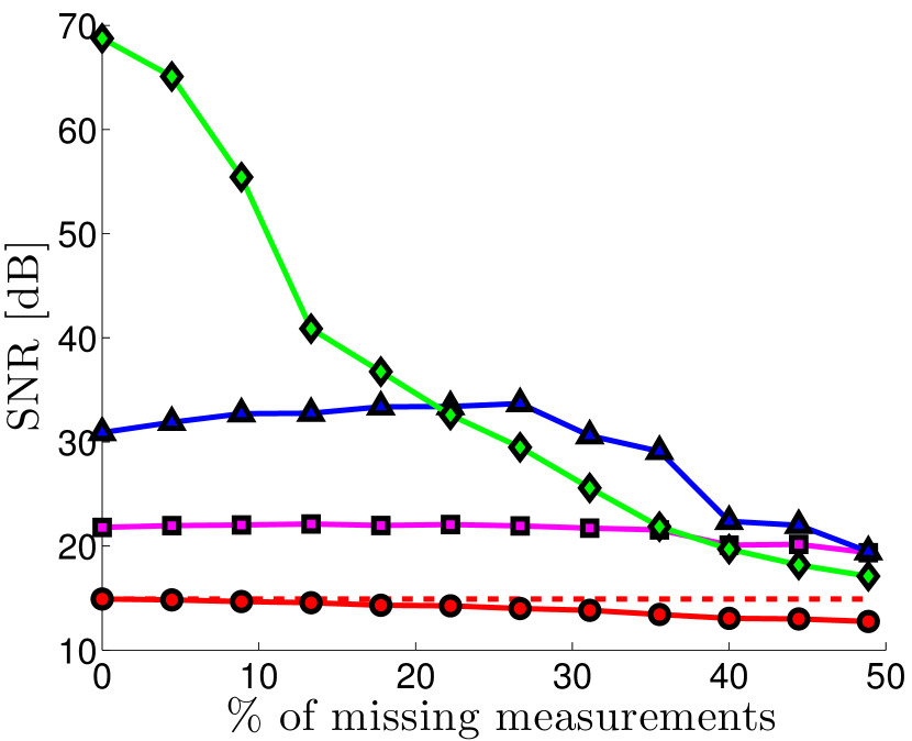
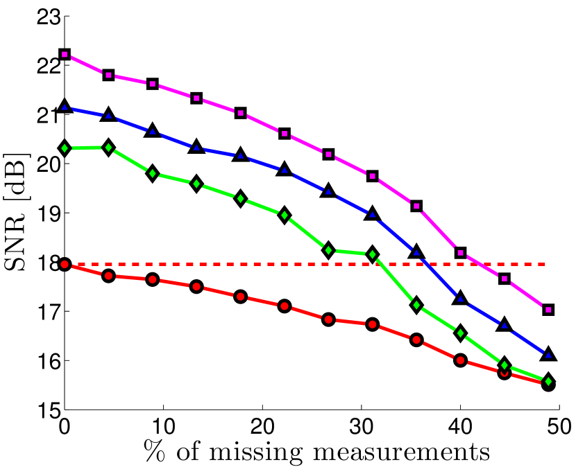
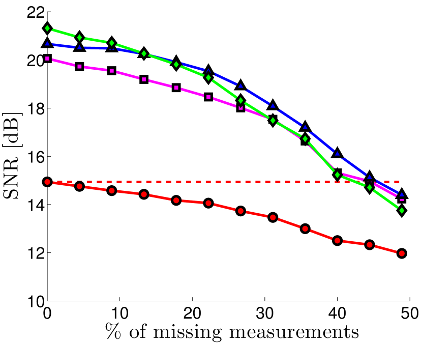
As it can be seen in Fig. 6(a), 6(c), 7(a), and 7(c), when there are a low number of outliers (2 in this case), the best results are obtained for lower $k$ values. However, when the number of outliers increase, (Fig. 6(b), 6(d), 7(b) and 7(d), low $k$ values perform worse. So, we can conclude that $k$ must be a number as low as possible, but higher than the number of actual outliers.

Nevertheless, it is worth to observe the behaviour of Fig. 6(b), 6(d), 7(b) and 7(d) (with more outliers) when the percentage of missing data increases. It can be clearly seen that the lines corresponding to different values of $k$ are crossing among them. This seems to indicate that as the missing data percentage increases, the number of outliers that we are able to detect decreases.

Anyway, the results obtained by the Robust DeN+MC algorithm outperforms the Gauss-Markov estimator, asymptotically approaching it when the noise is very high. Note also that for high values of noise, the noise and the outliers are practically indistinguishable.

X Experiments with Real Data

The aim of this section is to evaluate whether the improvements obtained in section IX using synthetic data are actually found in real environments. To do this, the proposed algorithms have been evaluated using audio recordings from the AV16.3 database [40], an audio-visual corpus recorded in the Smart Meeting Room of the IDIAP Research Institute, in Switzerland. The same metrics and localization algorithm of the previous section has been employed.

Additionally, the proposed Robust DeN algorithm is compared with other recent state-of-the-art methods in section X-D. In that case, we have employed the same framework used in [8], wherein many methods were already compared. In order to make the comparison as fair as possible, in this part the localization algorithm will be the same as in [8].

X-A Experimental Setup

(a) IDIAP room layout showing the centered table, and the microphones arranged in two circular arrays.

(b) Positions evaluated in the real data experiments. Only the relevant room section is shown.

Figure 8: IDIAP Smart Meeting Room: experimental details.

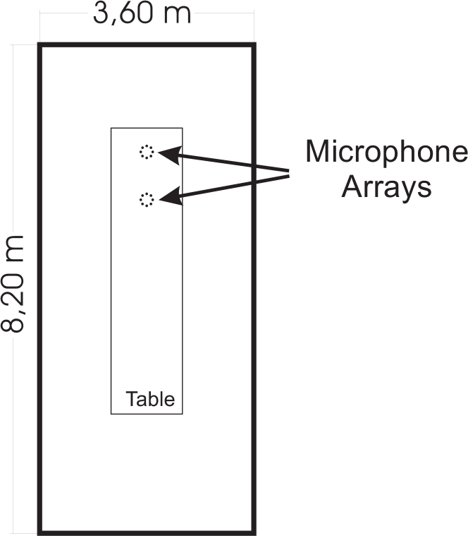
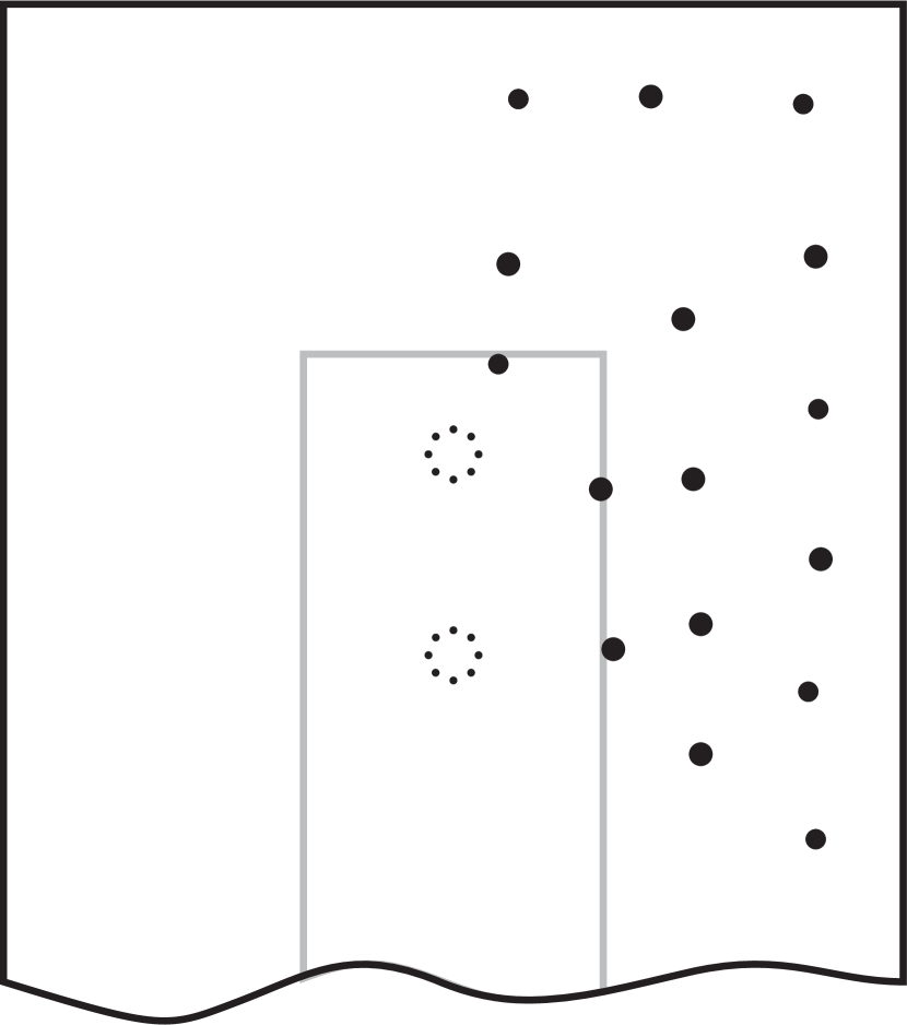
The IDIAP Meeting Room (shown in Fig. 8) is a $8.2m\times\nobreak 3.6m\times 2.4m$ rectangular space containing a centrally located $4.8m\times 1.2m$ rectangular table, on top of which two circular microphone arrays of $10cm$ radius are located, each of them composed by 8 microphones. The centers of the two arrays are separated by $80cm$ and the origin of coordinates is located in the middle point between the two arrays. A detailed description of the meeting room can be found in [41].

The audio recordings are synchronously sampled at $16~{}KHz$, and the complete database along with the corresponding annotation files containing the recordings ground truth (3D coordinates of the speaker’s mouth) is fully accessible on-line at [42]. It is composed by several sequences from which we are using sequence 01, with a single male speaker generating digit strings in 16 positions (which can be seen as small circles in Fig. 8(b)), distributed along the room. The sequence duration accounts for 208 seconds in total, with 823 ground truth frames.

The TDOA measurements $\Delta\tilde{\tau}_{ij}$, from which the measured TDOA matrix $\mathbf{\tilde{M}}$ is built, where estimated using the highest peak of the GCC-PHAT function[26].

As in a real scenario outliers are common but difficult to anticipate or enforce, the sweep over noise levels and the number of outliers that we performed with synthetic data are not feasible. Therefore, in our experiments with real data, we will only provide the SNR values and localization errors obtained after using each algorithm.

X-B Evaluation of Robust TDOA Denoising

In this experiment, all the microphone pairs have been considered, hence 120 TDOA values have been computed for each frame.

In table I we show an example of the results for the Robust DeN algorithm with $k=10$. As it also happened with synthetic data, in this case the proposed algorithm outperforms the Gauss-Markov estimator, yielding great improvements in both SNR and localization precision. Fig. 9 shows that the selection of $k$ is not very critical in this dataset as improvements over Gauss-Markov are obtained for a wide range of $k$.

TABLE I: Robust denoising performance in real data

	SNR (dB)	Average Localization error (mm)
Robust DeN	27.46	354
Gauss-Markov	23.19	515
Only non-redundant set	17.83	858

.

These results are the baseline for the experiments with missing data described in the next subsection.

X-C Evaluation of Robust TDOA Denoising with Missing Data

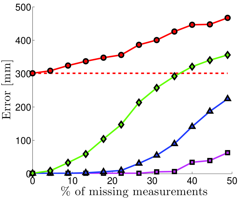
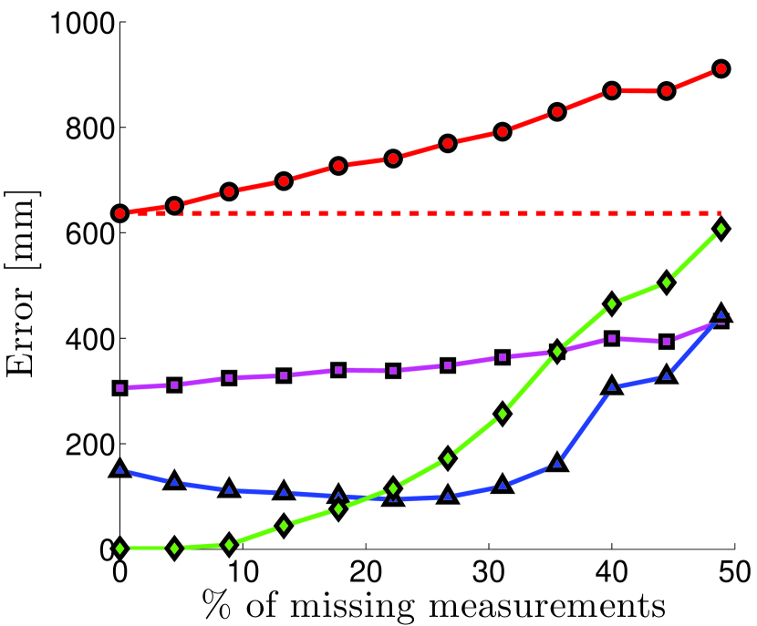
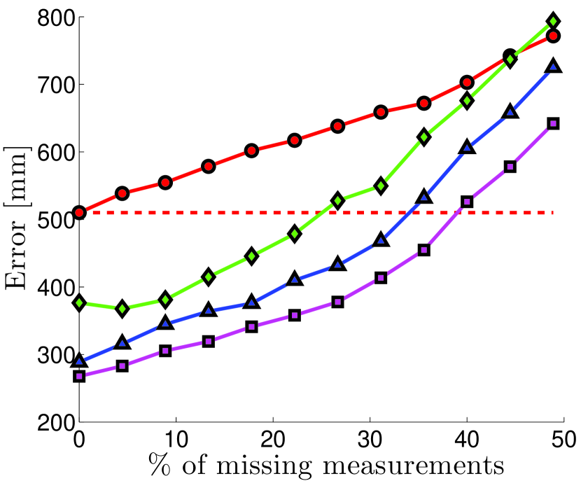
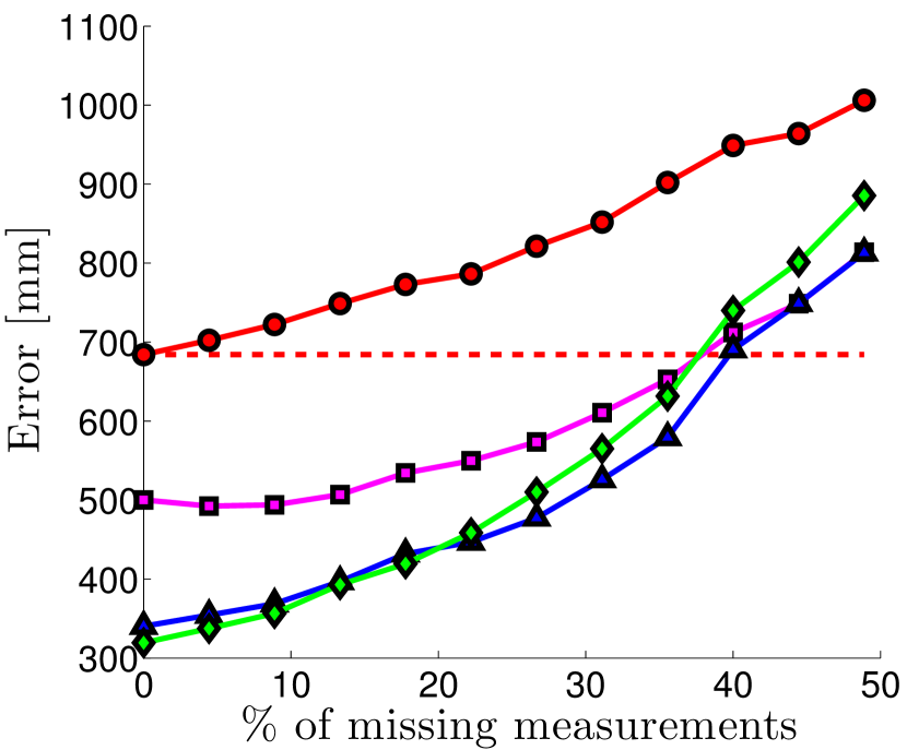
In the second experiment with real data, we randomly remove a set of TDOA measurements. Fig. 9 shows the obtained results. The dotted lines correspond to the performance (SNR and localization error) achieved by the Gauss-Markov estimator when there are no missing measurements. The solid lines with circular marks are the results obtained by the MC algorithm described in section VII.

On the other hand, the solid lines with squared/triangular/diamond marks correspond with the results of the Robust DeN+MC algorithm presented in section VIII. The different colors/shapes indicate different values of the hyperparameter $k$.

(a) SNR in dB

(b) Localization error in mm (using [16])

Figure 9: Results for real data with missing TDOA measurements.

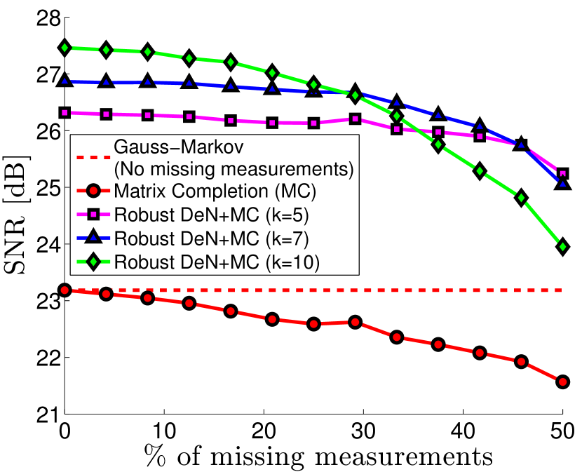
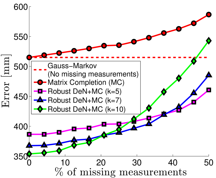
Fig. 9 highlights the relevance of the proposed robust-denoising algorithm (Robust DeN+MC) in real-scenarios, with important improvements over its non robust version (MC): higher than 4dB absolute improvement in terms of SNR, and around 30% relative improvement (15 cm absolute) in terms of localization precision.

We again observe that as the percentage of missing data increases, the lines corresponding to different values of $k$ are crossing among them. This behaviour is very similar to that found in the synthetic experiments above (refer to Fig. 6 and Fig. 7) for a high number of outliers, what suggests that this is the case in the real experiment, also serving as a validation for our simulation conclusions.

It is also noteworthy that, in order to get the best result, the maximum number of outliers $k$ should be decreased when the number of missing measurements increases.

X-D Comparison with Other Methods in a Localization Task

In this section we made use of the code and real data of the gtde MATLAB toolbox [43, 8]. In this toolbox, real recordings were performed under noisy conditions in a 4x4x4 (m) room, in which an array of 4 microphones forming a tetrahedron of 20 cm side has been placed. Sound waves coming from a loudspeaker placed at 189 different locations 1.7 m away from the array were recorded at 48 KHz.

Table II shows the results of the different algorithms on the localization task. The first 5 columns refer to the results of the Robust DeN algorithm for 5 different values of the parameter $k$. The rest of the columns show the results of a selection of the algorithms implemented and evaluated in [8] (the nomenclature has been kept and the results are essentially the same).

From [8], we selected three multilateration methods (generically referred to as x-mult) which are implementations of the algorithm described in [44]. These methods require to be initialized with the distance $r$ to the source. They were selected because they also make use of the redundancy between all the correlations, using the same input as the Robust DeN algorithm. We also compare our proposal with the branch & bound (b&b) method proposed by the authors of [8], as this is the one with the best performance in that work. The interested reader may refer to [8] for further details about the used methods, and the results of some other methods as well.

The Robust DeN algorithm is the only one of the evaluated algorithms that does not require information about the array geometry to perform denoising of the TDOA estimations. The localization algorithm (i.e converting TDOA to angles), implemented in [43], was used after all the methods in order to make the comparison as fair as possible.

The first row in table II shows the percentage of localization measurements with an angular error lower than 30º, the second row shows their mean angular error, and the third row their standard deviation.

TABLE II: Real data performance comparison between Robust DeN and selected algorithms in [8] (marked with ^∗) ($T_{60}\approx 0.5s$)

	Robust DeN					n-mult∗	t-mult∗	f-mult∗	b&b∗
	$k=0$	$k=1$	$k=2$	$k=3$	$k=4$
% Measurements with angular error $<30^{\circ}$	23.78%	24.12%	25.20%	25.71%	23.52%	13.99%	17.38%	17.91%	27.60%
Mean angular error	17.21	16.44	16.60	16.78	17.66	17.08	16.05	15.25	16.89
Standard deviation of angular error	7.52	7.44	7.52	7.52	7.38	7.31	7.80	7.78	7.50

To complement the data of Table II, we have also evaluated the execution timing details of the evaluated algorithms, with the results shown in Table III.

Table II shows that the Robust DeN algorithm performs better than the x-mult algorithms. Note that this happens even when the input data is the same, and neither the geometry of the array, nor the distance to the source $r$ are used for denonising in our proposal. In what respect to computational demands, our proposal is over 50 times faster.

Comparing with the b&b algorithm, our proposal is close to its performance, which is also an important result provided that (again) we do not use the array geometry for denoising, and our execution time is over 110 times faster.

TABLE III: Average execution time (s) and standard deviation for each method (evaluated on 9435 trials).

	Robust DeN	x-mult	b&b
Mean time (s)	0.024	1.255	2.649
Std (s)	0.0011	0.086	0.339

XI Conclusions

This paper has studied the properties of TDOA matrices, showing that they can be effectively used for solving TDOA denoising problems. In particular, the paper has investigated challenging scenarios where the TDOA matrix is contaminated with Gaussian noise, outliers and where a percentage of the measurements are missing. The paper shows that denoising in the presence of Gaussian noise and missing data can be solved in closed-form. This result is important, as it is the basis of an iterative algorithm that can also cope with outliers. The paper has tested the proposed algorithms in the context of acoustic localization using microphone arrays. The experimental results, both on real and synthetic data have shown that our algorithms successfully perform denoising (up to 30% of improvement in localization accuracy) with a high rate of missing data (up to 50%) and outliers, without knowing the sensor positions. This is important as it opens its application to tasks where the sensors geometry is unknown. Interestingly, in real datasets our robust denoising algorithm is systematically better than the Gauss-Markov estimator even when there is no missing data. This is also an important result as it proves that the assumption of Gaussian noise does not hold in real cases, while our robust model is capable of automatically discard erroneous measurements. The proposed robust denoising method has also been compared with other methods in literature on a localization task. Our results are very similar to the state of the art, even though we do not require knowing the array geometry in the denoising stage. Furthermore, our proposal is significantly less computationally demanding.

As for future work, we plan to further test our denoising algorithms in applications where the position of the sensors is unknown in advance, such in self-localization and beamforming.

References

- [1] X. Sheng and Y.-H. Hu, “Maximum likelihood multiple-source localization using acoustic energy measurements with wireless sensor networks,” IEEE Transactions on Signal Processing, vol. 53, no. 1, pp. 44 – 53, jan. 2005.
- [2] Y. Kuang and K. Astrom, “Stratified sensor network self-calibration from TDOA measurements,” in Signal Processing Conference (EUSIPCO), 2013 Proceedings of the 21st European. IEEE, 2013, pp. 1–5.
- [3] X. Anguera, C. Wooters, and J. Hernando, “Acoustic beamforming for speaker diarization of meetings,” Audio, Speech, and Language Processing, IEEE Transactions on, vol. 15, no. 7, pp. 2011–2022, 2007.
- [4] M. Brandstein and D. Ward, Eds., Microphone Arrays : Signal Processing Techniques and Applications. Springer, 2001.
- [5] G. C. Carter et al., “Special issue on time delay estimation,” in IEEE Trans. Acoust., Speech, Sig. Process., G. C. Carter, Ed., Jun 1981, vol. ASSP-29, no. 3, pp. 461 – 624.
- [6] J. Chen, J. Benesty, and Y. Huang, “Time delay estimation in room acoustic environments: an overview,” EURASIP Journal on applied signal processing, vol. 2006, pp. 170–170, 2006.
- [7] K. Ho, “Bias reduction for an explicit solution of source localization using TDOA,” Signal Processing, IEEE Transactions on, vol. 60, no. 5, pp. 2101–2114, 2012.
- [8] X. Alameda-Pineda and R. Horaud, “A geometric approach to sound source localization from time-delay estimates,” Audio, Speech, and Language Processing, IEEE/ACM Transactions on, vol. 22, no. 6, pp. 1082–1095, 2014.
- [9] M. Compagnoni, R. Notari, F. Antonacci, and A. Sarti, “A comprehensive analysis of the geometry of TDOA maps in localization problems,” Inverse Problems, vol. 30, no. 3, p. 035004, 2014.
- [10] A. Nouvellet, M. Charbit, F. Roueff, and A. Le Pichon, “Slowness estimation from noisy time delays observed on non-planar arrays,” Geophysical Journal International, vol. 198, no. 2, pp. 1199–1207, 2014.
- [11] B. Huang, L. Xie, and Z. Yang, “TDOA-based source localization with distance-dependent noises,” Wireless Communications, IEEE Transactions on, vol. 14, no. 1, pp. 468–480, 2015.
- [12] J. DiBiase, H. Silverman, and M. Brandstein, “Robust localization in reverberant rooms,” in Microphone Arrays, ser. Digital Signal Processing, M. Brandstein and D. Ward, Eds. Springer Berlin Heidelberg, 2001, pp. 157–180. [Online]. Available: http://dx.doi.org/10.1007/978-3-662-04619-7_8
- [13] B. Yang and J. Scheuing, “A theoretical analysis of 2D sensor arrays for TDOA based localization,” in Acoustics, Speech and Signal Processing, 2006. ICASSP 2006 Proceedings. 2006 IEEE International Conference on, vol. 4. IEEE, 2006, pp. IV–IV.
- [14] W. Hahn and S. Tretter, “Optimum processing for delay-vector estimation in passive signal arrays,” Information Theory, IEEE Transactions on, vol. 19, no. 5, pp. 608–614, Sep 1973.
- [15] N. Zhu, “Locating and extracting acoustic and neural signals,” Wayne State University, Dissertation 422, 2011. [Online]. Available: http://digitalcommons.wayne.edu/oa_dissertations/422
- [16] Y. Chan and K. Ho, “A simple and efficient estimator for hyperbolic location,” Signal Processing, IEEE Transactions on, vol. 42, no. 8, pp. 1905–1915, 1994.
- [17] M. Pollefeys and D. Nister, “Direct computation of sound and microphone locations from time-difference-of-arrival data.” in ICASSP, 2008, pp. 2445–2448.
- [18] J. O. Smith and J. S. Abel, “Closed-form least-squares source location estimation from range-difference measurements,” Acoustics, Speech and Signal Processing, IEEE Transactions on, vol. 35, no. 12, pp. 1661–1669, 1987.
- [19] M. D. Gillette and H. F. Silverman, “A linear closed-form algorithm for source localization from time-differences of arrival,” Signal Processing Letters, IEEE, vol. 15, pp. 1–4, 2008.
- [20] Y. Weng, W. Xiao, and L. Xie, “Total least squares method for robust source localization in sensor networks using TDOA measurements,” International Journal of Distributed Sensor Networks, vol. 2011, 2011.
- [21] L. Lin, H.-C. So, F. K. Chan, Y. Chan, and K. Ho, “A new constrained weighted least squares algorithm for TDOA-based localization,” Signal Processing, vol. 93, no. 11, pp. 2872–2878, 2013.
- [22] H. Jamali-Rad and G. Leus, “Sparsity-aware multi-source TDOA localization,” Signal Processing, IEEE Transactions on, vol. 61, no. 19, pp. 4874–4887, 2013.
- [23] H. C. So, Y. T. Chan, and F. Chan, “Closed-form formulae for time-difference-of-arrival estimation,” Signal Processing, IEEE Transactions on, vol. 56, no. 6, pp. 2614–2620, June 2008.
- [24] A. Renaux, P. Forster, E. Boyer, and P. Larzabal, “Unconditional maximum likelihood performance at finite number of samples and high signal-to-noise ratio,” Signal Processing, IEEE Transactions on, vol. 55, no. 5, pp. 2358–2364, 2007.
- [25] R. Schmidt, “Least squares range difference location,” Aerospace and Electronic Systems, IEEE Transactions on, vol. 32, no. 1, pp. 234–242, Jan 1996.
- [26] C. Knapp and G. Carter, “The generalized correlation method for estimation of time delay,” IEEE Transactions on Acoustics, Speech and Signal Processing, vol. 24, no. 4, pp. 320 – 327, aug 1976.
- [27] C. Zhang, D. Florencio, and Z. Zhang, “Why does PHAT work well in low noise, reverberative environments?” in Proceedings of ICASSP 2008, 31 2008-april 4 2008, pp. 2565 –2568.
- [28] J. Velasco, C. J. Martín-Arguedas, J. Macias-Guarasa, D. Pizarro, and M. Mazo, “Proposal and validation of an analytical generative model of SRP-PHAT power maps in reverberant scenarios,” Signal Processing, vol. 119, pp. 209 – 228, 2016. [Online]. Available: http://www.sciencedirect.com/science/article/pii/S0165168415002650
- [29] J. Benesty, “Adaptive eigenvalue decomposition algorithm for passive acoustic source localization,” The Journal of the Acoustical Society of America, vol. 107, no. 1, pp. 384–391, 2000.
- [30] J. Scheuing and B. Yang, “Disambiguation of TDOA estimation for multiple sources in reverberant environments,” Audio, Speech, and Language Processing, IEEE Transactions on, vol. 16, no. 8, pp. 1479–1489, 2008.
- [31] P. Annibale, J. Filos, P. Naylor, R. Rabenstein et al., “TDOA-based speed of sound estimation for air temperature and room geometry inference,” Audio, Speech, and Language Processing, IEEE Transactions on, vol. 21, no. 2, pp. 234–246, 2013.
- [32] M. Compagnoni, A. Canclini, P. Bestagini, F. Antonacci, A. Sarti, and S. Tubaro, “TDOA denoising for acoustic source localization,” CoRR, vol. abs/1509.02380, 2015. [Online]. Available: http://arxiv.org/abs/1509.02380
- [33] G. Ye, D. Liu, I.-H. Jhuo, and S.-F. Chang, “Robust late fusion with rank minimization,” in Computer Vision and Pattern Recognition (CVPR), 2012 IEEE Conference on. IEEE, 2012, pp. 3021–3028.
- [34] C. Eckart and G. Young, “The approximation of one matrix by another of lower rank,” Psychometrika, vol. 1, no. 3, pp. 211–218, 1936.
- [35] L. Mirsky, “Symmetric gauge functions and unitarily invariant norms,” The quarterly journal of mathematics, vol. 11, no. 1, pp. 50–59, 1960.
- [36] E. J. Candès, X. Li, Y. Ma, and J. Wright, “Robust principal component analysis,” Journal of the ACM (JACM), vol. 58, no. 3, p. 11, 2011.
- [37] T. Zhou and D. Tao, “GoDec: Randomized low-rank & sparse matrix decomposition in noisy case,” in in International Conference on Machine Learning, 2011.
- [38] A. Goldberg, B. Recht, J. Xu, R. Nowak, and X. Zhu, “Transduction with matrix completion: Three birds with one stone,” in Advances in Neural Information Processing Systems 23, J. D. Lafferty, C. K. I. Williams, J. Shawe-Taylor, R. S. Zemel, and A. Culotta, Eds. Curran Associates, Inc., 2010, pp. 757–765. [Online]. Available: http://papers.nips.cc/paper/3932-transduction-with-matrix-completion-three-birds-with-one-stone.pdf
- [39] E. J. Candès and T. Tao, “The power of convex relaxation: Near-optimal matrix completion,” IEEE Trans. Inf. Theor., vol. 56, no. 5, pp. 2053–2080, May 2010. [Online]. Available: http://dx.doi.org/10.1109/TIT.2010.2044061
- [40] G. Lathoud, J.-M. Odobez, and D. Gatica-Perez, “AV16.3: An audio-visual corpus for speaker localization and tracking,” in Procceedings of the MLMI, ser. Lecture Notes in Computer Science, S. Bengio and H. Bourlard, Eds., vol. 3361. Springer-Verlag, 2004, pp. 182–195.
- [41] D. C. Moore, “The IDIAP smart meeting room,” IDIAP Research Institute, Switzerland, Tech. Rep., November 2004.
- [42] G. Lathoud, “AV16.3 dataset,” http://www.idiap.ch/dataset/av16-3/, [Last accessed in december 2015].
- [43] X. Alameda-Pineda, “The gtde matlab toolbox.” [Online]. Available: https://team.inria.fr/perception/the-gtde-matlab-toolbox/
- [44] M. S. Brandstein and H. F. Silverman, “A practical methodology for speech source localization with microphone arrays,” Computer Speech & Language, vol. 11, no. 2, pp. 91–126, 1997.